Training a Classification Model to Detect Suspected Tumors
- 1. The Cancer Detection Pipeline: Focusing on Classification
- 2. High-Level Training Application Architecture (
LunaTrainingApp) - 3. Pretraining Setup: DataLoaders and Device Management
- 4. 3D Convolutional Neural Network Design (
LunaModel) - 5. Training and Validation Engine
- 6. Metric Tracking and Clinical Performance Logging
- 7. Real-Time Telemetry with TensorBoard
- 8. The Accuracy Paradox: 99.7% Correct and Total Clinical Failure
- 9. Summary and Engineering Principles

1. The Cancer Detection Pipeline: Focusing on Classification
In Section 2.4, we engineered the data ingestion foundation for our clinical diagnostic system: parsing raw thoracic CT scans (.mhd/.raw), mapping continuous millimeter coordinates into discrete voxel matrix indices ($[I, R, C]$), and slicing normalized 3D sub-volume patches ($32 \times 32 \times 32$ voxels) centered on suspicious tissue candidates.
This brings us to Step 3: Nodule Classification in the overall clinical pipeline.
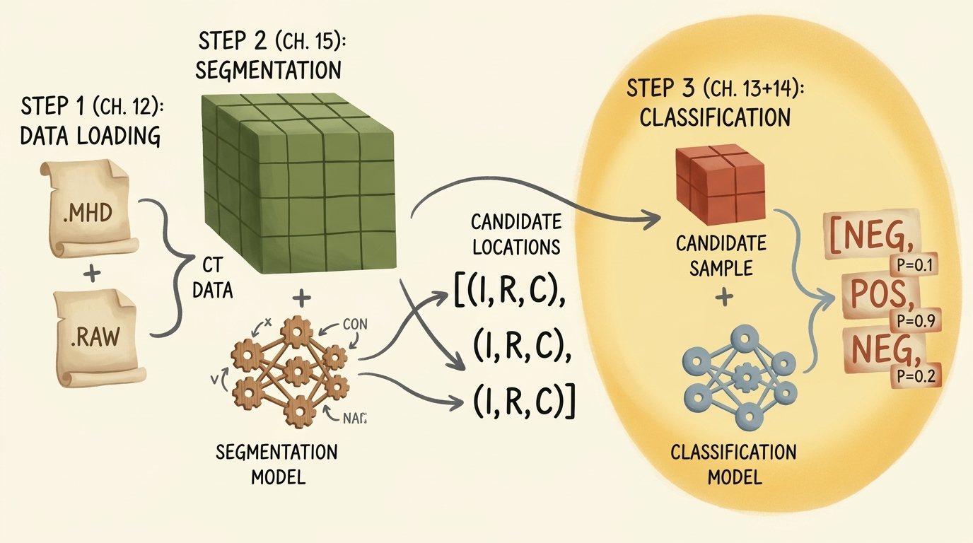
flowchart TD
    subgraph Pipeline ["End-to-End Clinical System"]
        direction TB
        S1["Step 1 (Ch. 12): Volumetric Data Ingestion<br/>CT Reconstruction & Voxel Patch Extraction"]
        S2["Step 2 (Ch. 15): Candidate Segmentation<br/>U-Net Anatomical Region Proposals"]
        S3["Step 3 (Ch. 13 & 14): Nodule Classification<br/>3D CNN Binary Malignancy Discriminator"]
        S1 --> S2 --> S3
    end

    style Pipeline fill:#1a1a2e,stroke:#4cc9f0,stroke-width:2px,color:#fff
    style S1 fill:#16213e,stroke:#4cc9f0,stroke-width:1px,color:#fff
    style S2 fill:#1a3a2a,stroke:#52b788,stroke-width:1px,color:#fff
    style S3 fill:#3a1a1a,stroke:#e63946,stroke-width:2px,color:#fff
Our primary objective in this module is binary classification: given an extracted volumetric tensor patch of shape $(1, 32, 32, 32)$, predict whether the candidate tissue represents an actual tumor nodule ($y = 1$) or benign non-nodule anatomy ($y = 0$, such as vascular junctions, bronchial walls, or bone spurs).
2. High-Level Training Application Architecture (LunaTrainingApp)
Production-grade deep learning systems require clean, reproducible architectural separation rather than sprawling scripts. We encapsulate the entire training and validation lifecycle within an object-oriented application class: LunaTrainingApp.
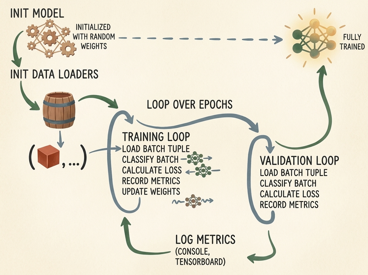
The execution lifecycle follows a structured sequence:
- Command-Line Parsing (
__init__): Parse runtime hyperparameters via Python’s standardargparsemodule (--batch-size,--epochs,--num-workers,--lr). - Resource Setup (
initModel,initOptimizer): Initialize neural network architecture, instantiate optimizers, and bind memory to CUDA or CPU devices. - Data Pipeline Initialization (
initDataLoaders): Build training and validation data loaders with zero-leakage cross-validation grouping. - Epoch Iteration (
main): For each epoch, execute an active gradient-updated training loop (doTraining), followed by an evaluation loop (doValidation) and telemetry logging (logMetrics).
2.1 The Application Scaffold
Let us implement the foundational structure of the training application class:
import argparse
import datetime
import sys
import torch
import torch.nn as nn
from torch.utils.data import DataLoader
from torch.optim import SGD

class LunaTrainingApp:
    def __init__(self, sys_argv=None):
        if sys_argv is None:
            sys_argv = sys.argv[1:]

        parser = argparse.ArgumentParser(
            description="Train 3D CNN Nodule Classifier on LUNA Dataset."
        )
        parser.add_argument(
            '--batch-size',
            help='Batch size to use for training',
            default=32,
            type=int,
        )
        parser.add_argument(
            '--num-workers',
            help='Number of worker processes for background data loading',
            default=4,
            type=int,
        )
        parser.add_argument(
            '--epochs',
            help='Number of epochs to train',
            default=1,
            type=int,
        )
        parser.add_argument(
            '--tb-prefix',
            default='p2ch13',
            help="Prefix for TensorBoard run directory",
        )
        parser.add_argument(
            '--comment',
            help="Comment suffix for TensorBoard run name",
            nargs='?',
            default='dwlpt',
        )

        self.cli_args = parser.parse_args(sys_argv)
        self.time_str = datetime.datetime.now().strftime('%Y-%m-%d_%H.%M.%S')
        self.use_cuda = torch.cuda.is_available()
        self.device = torch.device("cuda" if self.use_cuda else "cpu")
The parameters configured here dictate physical execution:
self.use_cudachecks hardware acceleration. When a CUDA-capable GPU is available, all model weights and input tensor batches are staged into GPU VRAM.self.time_strgenerates an immutable timestamp string for logging directory names, ensuring that different experimental runs never overwrite one another.
3. Pretraining Setup: DataLoaders and Device Management
The preparation phase establishes model weights and data access channels before entering iterative gradient descent.
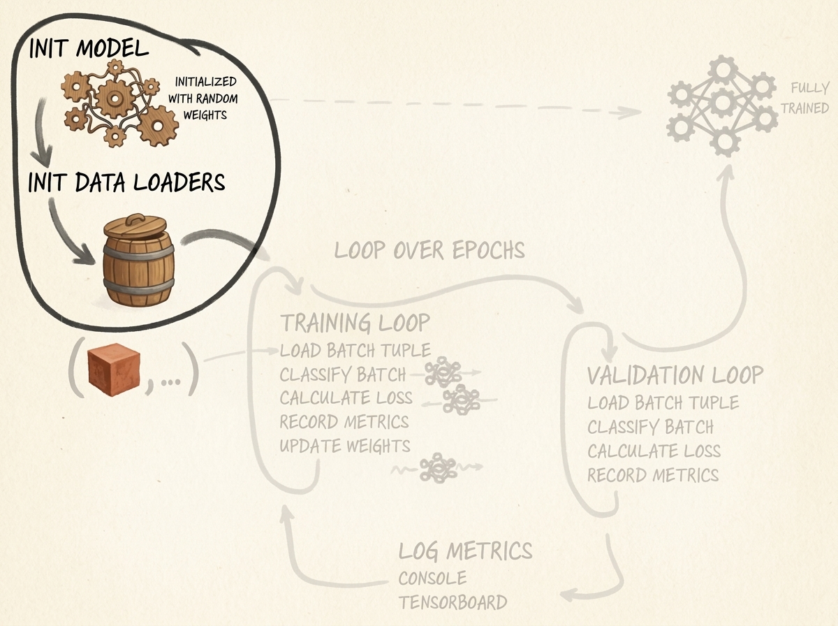
3.1 Initializing the Model and Optimizer
We instantiate the model and move its parameters to the chosen device. We select Stochastic Gradient Descent (SGD) with classical momentum and weight decay:
    def initModel(self):
        model = LunaModel()
        if self.use_cuda:
            print(f"Using CUDA device: {torch.cuda.get_device_name(0)}")
            if torch.cuda.device_count() > 1:
                model = nn.DataParallel(model)
            model = model.to(self.device)
        return model

    def initOptimizer(self):
        return SGD(self.model.parameters(), lr=0.001, momentum=0.99)
Note
Setting momentum to
0.99creates substantial exponential averaging of previous gradient vectors: $$ \mathbf{v}_{t} = \mu \mathbf{v}_{t-1} + \mathbf{g}_t, \quad \mathbf{\theta}_{t} = \mathbf{\theta}_{t-1} - \alpha \mathbf{v}_t $$ In sparse gradients where positive nodule samples appear infrequently, high momentum helps push parameters through plateaus, although as we will observe later, this alone cannot overcome extreme class imbalance.
3.2 Care and Feeding of 3D DataLoaders
Each individual call to LunaDataset.__getitem__ yields a 4-element tuple containing a 4D tensor (1, 32, 32, 32), a boolean nodule flag, patient series UID, and physical center coordinate. The DataLoader collates these individual items into batched tensors.
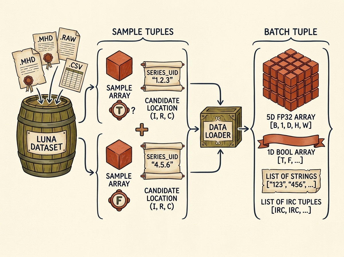
    def initTrainDl(self):
        train_ds = LunaDataset(
            val_stride=10,
            is_val_set_bool=False,
        )
        batch_size = self.cli_args.batch_size
        if self.use_cuda:
            batch_size *= torch.cuda.device_count()

        train_dl = DataLoader(
            train_ds,
            batch_size=batch_size,
            num_workers=self.cli_args.num_workers,
            pin_memory=self.use_cuda,
        )
        return train_dl

    def initValDl(self):
        val_ds = LunaDataset(
            val_stride=10,
            is_val_set_bool=True,
        )
        batch_size = self.cli_args.batch_size
        if self.use_cuda:
            batch_size *= torch.cuda.device_count()

        val_dl = DataLoader(
            val_ds,
            batch_size=batch_size,
            num_workers=self.cli_args.num_workers,
            pin_memory=self.use_cuda,
        )
        return val_dl
Memory & Performance Optimizations:
pin_memory=True: Instructs the runtime to allocate host tensors in page-locked (pinned) system memory. When copying from pinned CPU RAM to CUDA GPU VRAM via.to(self.device, non_blocking=True), the transfer occurs asynchronously via Direct Memory Access (DMA) over the PCIe bus without involving the host CPU core.num_workers=4: Spawns separate worker processes that execute Python unpickling, disk caching lookups, and tensor conversions in parallel background processes, avoiding GPU starvation.val_stride=10: Implements 10-fold patient grouping cross-validation where all candidates belonging to every 10th patient volume are reserved for validation, guaranteeing strict zero data leakage.
4. 3D Convolutional Neural Network Design (LunaModel)
4.1 3D Convolutions: Geometric & Computational Mechanics
In standard 2D image processing, a convolution kernel slides over height and width axes: $(C_{\text{in}}, H, W) \to (C_{\text{out}}, H’, W’)$. In volumetric medical imaging, anatomical nodules are intrinsically 3-dimensional spherical or ellipsoidal structures spanning multiple CT axial slices. Analyzing 2D slices independently discards the critical cross-slice contextual gradient.
A 3D convolution layer (nn.Conv3d) slides a 3D kernel filter across depth ($D$), height ($H$), and width ($W$):
$$ \text{Input Shape: } [N, C, D, H, W] $$
$$\mathbf{Y}_{n, c_{\text{out}}, d, h, w} = \mathbf{b}_{c_{\text{out}}} + \sum_{c_{\text{in}}=0}^{C_{\text{in}}-1} \sum_{i=0}^{K_d-1} \sum_{j=0}^{K_h-1} \sum_{k=0}^{K_w-1} \mathbf{K}_{c_{\text{out}}, c_{\text{in}}, i, j, k} \cdot \mathbf{X}_{n, c_{\text{in}}, d+i, h+j, w+k} $$
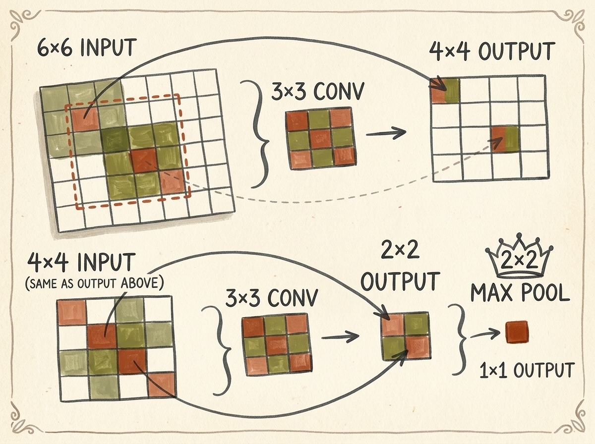
Parameter & Memory Scaling:
- A standard 2D kernel of size $3 \times 3$ contains $9$ weights per channel.
- A 3D kernel of size $3 \times 3 \times 3$ contains $27$ weights per channel—a threefold parameter increase.
- Crucially, activations scale with the volume: an intermediate tensor of shape $[32, 64, 16, 16, 16]$ contains $8{,}388{,}608$ single-precision floating-point elements, consuming $33.55\text{ MB}$ of VRAM for just one layer’s forward activations. Managing spatial downsampling via pooling is essential to prevent GPU out-of-memory crashes.
4.2 Architectural Anatomy of LunaModel
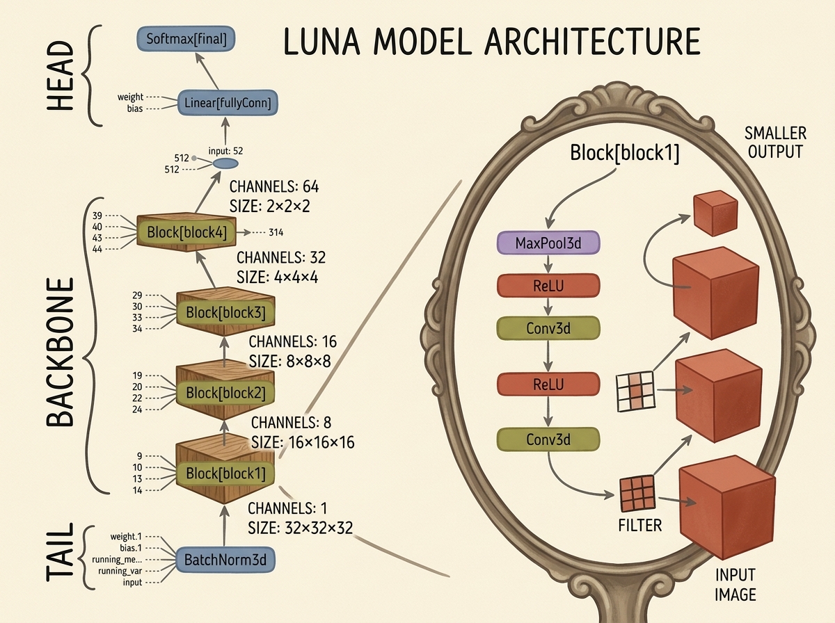
The architecture comprises three primary divisions:
- Tail: An initial
nn.BatchNorm3d(1)that normalizes raw input Hounsfield units on the fly, centering mean around $0$ and variance around $1$. - Backbone: A cascade of 4 modular
LunaBlocksub-networks, progressively increasing channel capacity ($1 \to 8 \to 16 \to 32 \to 64$) while halving spatial resolution at each stage via $2 \times 2 \times 2$ max pooling ($32^3 \to 16^3 \to 8^3 \to 4^3 \to 2^3$). - Head: A linear classification layer mapping the flattened $512$-dimensional embedding vector ($64 \times 2 \times 2 \times 2$) to $2$ output logits, followed by an explicit
nn.Softmax(dim=1)probability distribution: $[\hat{p}_{\text{non-nodule}}, \hat{p}_{\text{nodule}}]$.
4.3 Implementing LunaBlock and LunaModel
Let us construct the modular network:
class LunaBlock(nn.Module):
    def __init__(self, in_channels, conv_channels):
        super().__init__()

        self.conv1 = nn.Conv3d(
            in_channels, conv_channels, kernel_size=3, padding=1, bias=True
        )
        self.relu1 = nn.ReLU(inplace=True)
        self.conv2 = nn.Conv3d(
            conv_channels, conv_channels, kernel_size=3, padding=1, bias=True
        )
        self.relu2 = nn.ReLU(inplace=True)
        self.maxpool = nn.MaxPool3d(kernel_size=2, stride=2)

    def forward(self, input_batch):
        block_out = self.conv1(input_batch)
        block_out = self.relu1(block_out)
        block_out = self.conv2(block_out)
        block_out = self.relu2(block_out)
        return self.maxpool(block_out)
Each block maintains spatial dimensions across convolutions through padding=1, reserving all spatial compression for the subsequent nn.MaxPool3d(2, 2) operation.
Now we compose the complete model:
class LunaModel(nn.Module):
    def __init__(self):
        super().__init__()

        self.tail_batchnorm = nn.BatchNorm3d(1)

        self.block1 = LunaBlock(1, 8)
        self.block2 = LunaBlock(8, 16)
        self.block3 = LunaBlock(16, 32)
        self.block4 = LunaBlock(32, 64)

        self.head_linear = nn.Linear(64 * 2 * 2 * 2, 2)
        self.head_softmax = nn.Softmax(dim=1)

        self._init_weights()

    def _init_weights(self):
        for m in self.modules():
            if type(m) in {nn.Linear, nn.Conv3d}:
                nn.init.kaiming_normal_(
                    m.weight.data, a=0, mode='fan_out', nonlinearity='relu'
                )
                if m.bias is not None:
                    fan_in, _ = nn.init._calculate_fan_in_and_fan_out(m.weight.data)
                    bound = 1 / (fan_in ** 0.5)
                    nn.init.uniform_(m.bias.data, -bound, bound)

    def forward(self, input_batch):
        bn_output = self.tail_batchnorm(input_batch)

        conv1_out = self.block1(bn_output)
        conv2_out = self.block2(conv1_out)
        conv3_out = self.block3(conv2_out)
        conv4_out = self.block4(conv3_out)

        flattened = conv4_out.view(conv4_out.size(0), -1)
        linear_output = self.head_linear(flattened)

        return linear_output, self.head_softmax(linear_output)
Notice that forward returns two tensors:
linear_output(raw logits): passed directly to our loss function.self.head_softmax(linear_output)(probabilities): utilized for metric computation, logging, and downstream clinical decision rules.
5. Training and Validation Engine
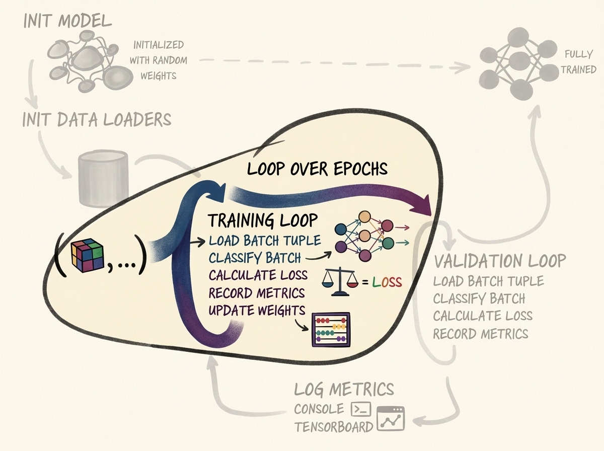
The training lifecycle alternates between gradient-driven parameter updates (doTraining) and detached evaluation (doValidation).
5.1 Computing Batch Loss (computeBatchLoss)
PyTorch’s nn.CrossEntropyLoss expects raw unnormalized logits rather than probabilities, internally combining nn.LogSoftmax with Negative Log-Likelihood (NLLLoss) for numerical stability:
$$ \mathcal{L}_{\text{batch}} = -\frac{1}{B} \sum_{i=1}^{B} \log \left( \frac{\exp(z_{i, y_i})}{\sum_{c=0}^1 \exp(z_{i, c})} \right) $$
    def computeBatchLoss(self, batch_ndx, batch_tup, batch_size, trn_metrics_g):
        input_t, label_t, _series_list, _center_list = batch_tup

        input_dev = input_t.to(self.device, non_blocking=True)
        label_dev = label_t.to(self.device, non_blocking=True)

        logits_dev, probability_dev = self.model(input_dev)

        loss_fn = nn.CrossEntropyLoss(reduction='none')
        loss_dev = loss_fn(logits_dev, label_dev)

        loss_bool = loss_dev.detach()
        probability_bool = probability_dev.detach()

        # Update per-sample telemetry tracking matrix
        start_ndx = batch_ndx * batch_size
        end_ndx = start_ndx + input_t.size(0)

        trn_metrics_g[0, start_ndx:end_ndx] = loss_bool
        trn_metrics_g[1, start_ndx:end_ndx] = probability_bool[:, 1]
        trn_metrics_g[2, start_ndx:end_ndx] = label_dev

        return loss_dev.mean()
Important
Always call
.detach()when storing loss values or probabilities into long-term history structures. Storing a live PyTorch tensor preserves its entire backward computational graph in memory, preventing garbage collection and rapidly exhausting system RAM.
5.2 Executing the Training Loop (doTraining)
    def doTraining(self, epoch_ndx, train_dl):
        self.model.train()
        trn_metrics_g = torch.zeros(
            3, len(train_dl.dataset), device=self.device
        )

        for batch_ndx, batch_tup in enumerate(train_dl):
            self.optimizer.zero_grad()

            loss_var = self.computeBatchLoss(
                batch_ndx, batch_tup, train_dl.batch_size, trn_metrics_g
            )

            loss_var.backward()
            self.optimizer.step()

        return trn_metrics_g.to('cpu')
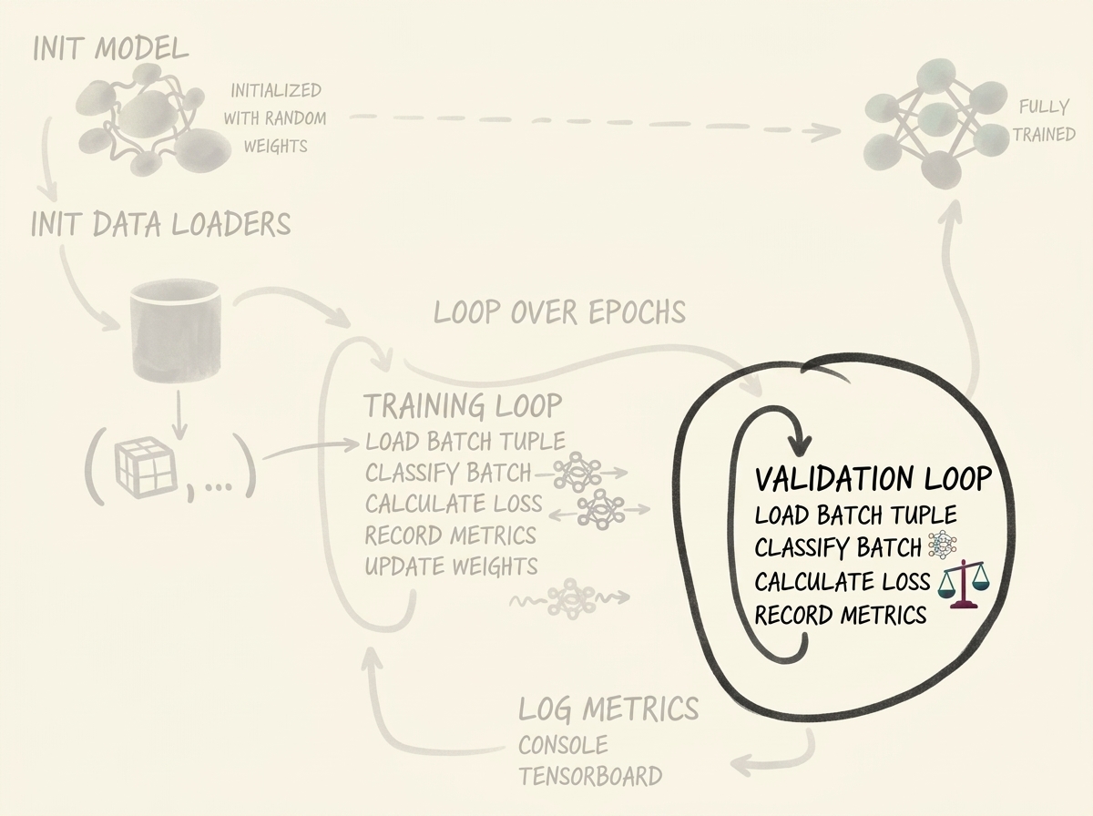
5.3 Executing the Validation Loop (doValidation)
In validation, backpropagation must be strictly inhibited to prevent gradient graph construction and reduce memory overhead:
    def doValidation(self, epoch_ndx, val_dl):
        with torch.inference_mode():
            self.model.eval()
            val_metrics_g = torch.zeros(
                3, len(val_dl.dataset), device=self.device
            )

            for batch_ndx, batch_tup in enumerate(val_dl):
                self.computeBatchLoss(
                    batch_ndx, batch_tup, val_dl.batch_size, val_metrics_g
                )

        return val_metrics_g.to('cpu')
6. Metric Tracking and Clinical Performance Logging
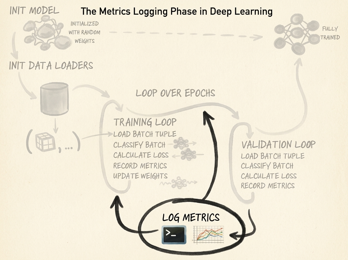
In medical diagnostic applications, overall classification accuracy is an actively hazardous metric. If $99.7%$ of candidates are non-nodules, a dummy model predicting $0$ for every sample achieves $99.7%$ accuracy while allowing $100%$ of malignant cancer patients to go untreated.
We must construct the full Confusion Matrix:
| Condition Positive (True Nodule) | Condition Negative (Benign) | |
|---|---|---|
| Predicted Positive | True Positive (TP) | False Positive (FP) |
| Predicted Negative | False Negative (FN) | True Negative (TN) |
From these four quadrants, we compute clinical diagnostic indicators:
- Sensitivity / Recall: What fraction of genuine nodules did we detect? $$ \text{Recall} = \frac{\text{TP}}{\text{TP} + \text{FN}} $$
- Precision / Positive Predictive Value: When the model flags a nodule, how often is it correct? $$ \text{Precision} = \frac{\text{TP}}{\text{TP} + \text{FP}} $$
- Specificity (True Negative Rate): How accurately does the system dismiss benign tissue? $$ \text{Specificity} = \frac{\text{TN}}{\text{TN} + \text{FP}} $$
- $F_1$-Score: The harmonic mean balancing precision and sensitivity: $$ F_1 = 2 \cdot \frac{\text{Precision} \cdot \text{Recall}}{\text{Precision} + \text{Recall}} $$
Let us implement logMetrics:
    def logMetrics(self, epoch_ndx, mode_str, metrics_t):
        negLabel_mask = metrics_t[2] == 0
        posLabel_mask = metrics_t[2] == 1

        negPred_mask = metrics_t[1] < 0.5
        posPred_mask = metrics_t[1] >= 0.5

        trueNeg_count = (negPred_mask & negLabel_mask).sum().item()
        falsePos_count = (posPred_mask & negLabel_mask).sum().item()
        truePos_count = (posPred_mask & posLabel_mask).sum().item()
        falseNeg_count = (negPred_mask & posLabel_mask).sum().item()

        total_count = len(metrics_t[0])
        correct_count = trueNeg_count + truePos_count

        total_pos = truePos_count + falseNeg_count
        total_neg = trueNeg_count + falsePos_count

        recall = truePos_count / (total_pos + 1e-8)
        precision = truePos_count / (truePos_count + falsePos_count + 1e-8)
        f1_score = 2 * (precision * recall) / (precision + recall + 1e-8)

        print(
            f"Epoch {epoch_ndx} {mode_str:8s} "
            f"Loss: {metrics_t[0].mean():.4f} | "
            f"Accuracy: {correct_count / total_count * 100:.2f}% | "
            f"Recall: {recall * 100:.2f}% | "
            f"Precision: {precision * 100:.2f}% | "
            f"F1: {f1_score:.4f}"
        )
        print(
            f"      TP: {truePos_count:5d} | FN: {falseNeg_count:5d} | "
            f"TN: {trueNeg_count:5d} | FP: {falsePos_count:5d}"
        )
7. Real-Time Telemetry with TensorBoard
Visualizing training dynamics allows immediate detection of divergence or vanishing gradients. We integrate PyTorch’s native torch.utils.tensorboard.SummaryWriter.
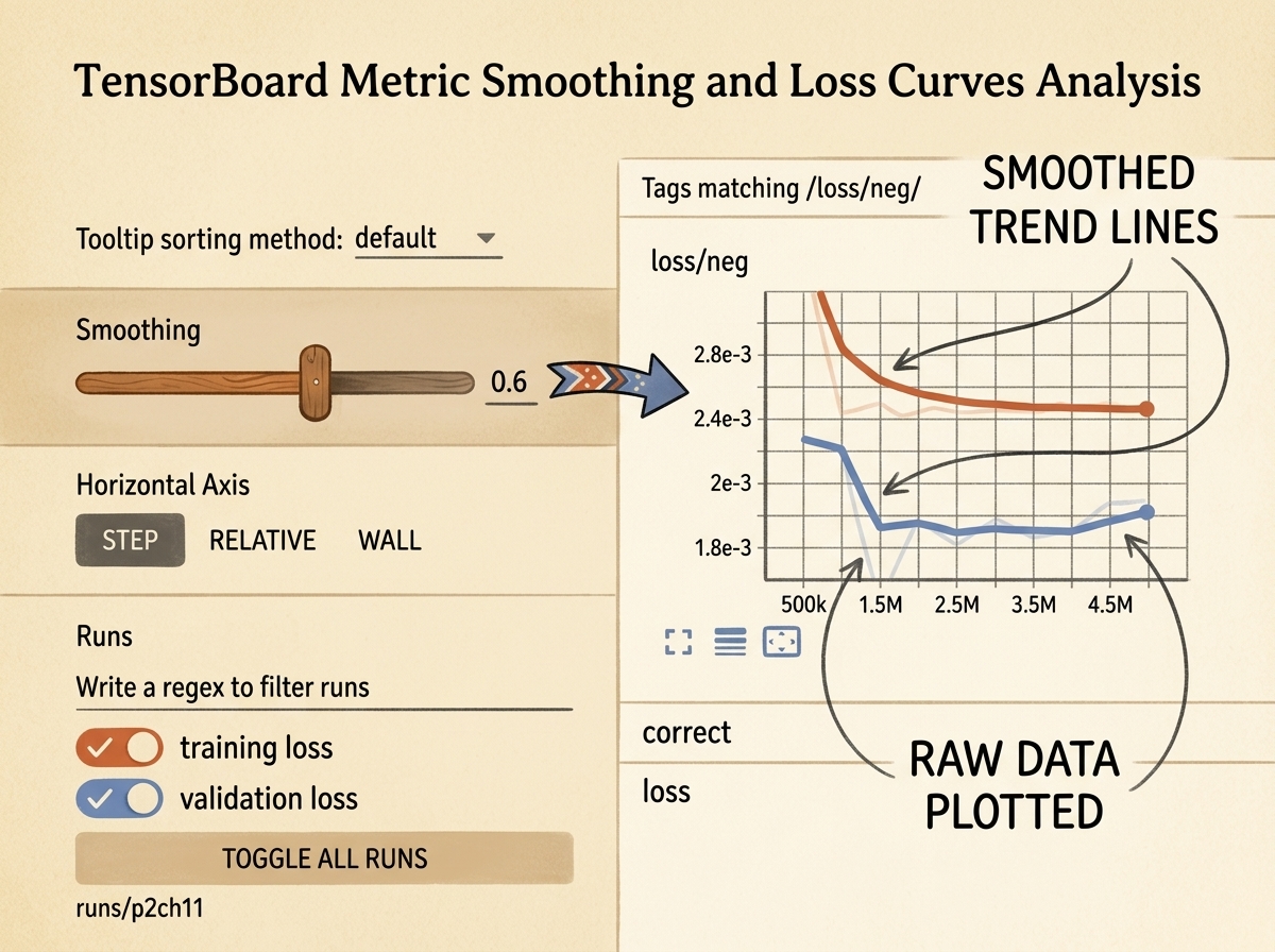
7.1 Initializing the SummaryWriter
from torch.utils.tensorboard import SummaryWriter

    def initTensorboard(self):
        log_dir = f"runs/{self.cli_args.tb_prefix}_{self.time_str}_{self.cli_args.comment}"
        self.trn_writer = SummaryWriter(log_dir=f"{log_dir}_trn")
        self.val_writer = SummaryWriter(log_dir=f"{log_dir}_val")
7.2 Writing Scalars to TensorBoard
During logMetrics, we push calculated indicators directly to event logs:
        writer = self.trn_writer if mode_str == 'train' else self.val_writer
        writer.add_scalar('loss/total', metrics_t[0].mean(), epoch_ndx)
        writer.add_scalar('accuracy/overall', correct_count / total_count, epoch_ndx)
        writer.add_scalar('clinical/recall', recall, epoch_ndx)
        writer.add_scalar('clinical/precision', precision, epoch_ndx)
        writer.add_scalar('clinical/f1_score', f1_score, epoch_ndx)
        writer.flush()
8. The Accuracy Paradox: 99.7% Correct and Total Clinical Failure
When we execute LunaTrainingApp across the dataset, the console displays a seemingly triumphant result:
Epoch 1 train    Loss: 0.0241 | Accuracy: 99.74% | Recall: 0.00% | Precision: 0.00% | F1: 0.0000
      TP:     0 | FN:  1351 | TN: 548649 | FP:     0
Epoch 1 val      Loss: 0.0238 | Accuracy: 99.76% | Recall: 0.00% | Precision: 0.00% | F1: 0.0000
      TP:     0 | FN:   149 | TN:  61251 | FP:     0
8.1 Anatomy of the Catastrophe
-
The Numbers:
- The model achieved an astonishing 99.74% overall accuracy.
- Yet out of $1{,}351$ cancer patients with true nodules, it detected exactly 0 (Zero TP, 1351 FN).
- True Positive Rate (Recall) = 0.00%.
-
Why Did Gradient Descent Choose This? Consider a standard mini-batch of size $32$: $$ \text{Expected Positives per Batch} = 32 \times \frac{1{,}351}{550{,}000} \approx 0.078 \text{ nodules} $$ Out of every $100$ batches processed by the GPU, approximately $92$ batches contain only negative non-nodule samples.
When backpropagation computes gradient vectors across the batch: $$ \nabla_{\mathbf{w}} \mathcal{L} = \frac{1}{B} \sum_{i=1}^B \nabla_{\mathbf{w}} \ell(f(\mathbf{x}_i), y_i) $$ For negative samples ($y_i = 0$), the loss pulls network outputs towards $[1.0, 0.0]$ (class $0$). Because negative samples outnumber positive samples by $400:1$, the sum of negative gradient vectors completely overwhelms and drowns out the occasional positive gradient signal.
The optimizer discovers the simplest, lowest-loss saddle point on the optimization landscape: predict class 0 constantly for all inputs.
flowchart TD
    subgraph ImbalanceTrap ["The Class Imbalance Gradient Trap"]
        direction TB
        B1["Batch N: 32 Benign Samples<br/>Pull weights toward Class 0"]
        B2["Batch N+1: 32 Benign Samples<br/>Pull weights toward Class 0"]
        B3["Batch N+2: 31 Benign + 1 Nodule<br/>Nodule signal drowned by 31 negative gradients"]
        B4["Trivial Local Minimum:<br/>Always predict P(Nodule) = 0.00<br/>Accuracy = 99.74% | Recall = 0.00%"]
        B1 --> B2 --> B3 --> B4
    end

    style ImbalanceTrap fill:#3a1a1a,stroke:#e63946,stroke-width:2px,color:#fff
    style B1 fill:#2a1a1a,stroke:#e63946,stroke-width:1px,color:#fff
    style B2 fill:#2a1a1a,stroke:#e63946,stroke-width:1px,color:#fff
    style B3 fill:#2a1a1a,stroke:#ffaa00,stroke-width:1px,color:#fff
    style B4 fill:#1a1a2e,stroke:#4cc9f0,stroke-width:2px,color:#fff
8.2 The Path Forward: Preview of Section 2.6 (Chapter 14)
Overcoming the Accuracy Paradox requires restructuring how our data loaders present reality to the neural network:
- Balanced Stratified Sampling: Enforcing a $1:1$ or $1:3$ ratio of positive nodules to negative samples in every single training batch, ensuring positive gradients have equal voice in weight updates.
- 3D Volumetric Data Augmentation: Because genuine nodules are scarce ($1{,}351$), synthesizing novel samples through 3D rotations, random flips, scaling, and spatial jittering to prevent catastrophic overfitting on balanced splits.
9. Summary and Engineering Principles
- 3D Convolutions Preserve Volumetric Context:
nn.Conv3dprocesses depth, height, and width simultaneously, expanding spatial receptive fields in three dimensions at the cost of cubic parameter and memory scaling. - Decouple Applications into Modular OOP: Isolating initialization (
initModel), data collation (initDataLoaders), loss computation (computeBatchLoss), and metrics tracking (logMetrics) makes training suites scalable and maintainable. - Zero Data Leakage: Ensure training and validation splits group samples by patient UID rather than randomly partitioning isolated candidate patches.
- Accuracy Is Unreliable Under Imbalance: In rare-event detection, high accuracy frequently masks total model collapse. Clinical systems must be evaluated using Confusion Matrices, Recall, Precision, and $F_1$-score.