Welcome
Deep Learning Notes
Notes taken during the Deep Learning Specialization
by Andrew Ng & Eddy Shyu
Stanford University & DeepLearning.AI
What I Built
| # | Course | Focus |
|---|---|---|
| 1 | Neural Networks and Deep Learning | Logistic regression as a neural network, shallow & deep networks, forward/backpropagation |
| 2 | Improving Deep Neural Networks | Hyperparameter tuning, regularization (Dropout, BatchNorm), optimization (Momentum, Adam), Xavier/He initialization |
| 3 | Structuring Machine Learning Projects | Train/dev/test splits, error analysis, transfer learning, end-to-end deep learning |
| 4 | Convolutional Neural Networks | CNNs, edge detection, classic & modern architectures (LeNet, AlexNet, VGG, ResNet, Inception, MobileNet, EfficientNet), object detection (YOLO), face recognition (FaceNet, Siamese), neural style transfer, U-Net |
| 5 | Sequence Models | RNNs, GRUs, LSTMs, word embeddings (Word2Vec, GloVe), attention models, Transformers, speech recognition, music synthesis, machine translation, chatbots |
— emreaslan —
Content
Welcome to Machine Learning notes.
∴
I completed the Machine Learning Specialization Course by taking detailed notes and summarizing critical concepts for future reference.
University of Stanford & DeepLearning.AI
— emreaslan —
Supervised and Unsupervised Machine Learning
Introduction
Machine learning is a branch of artificial intelligence that allows systems to learn and make predictions or decisions without explicit programming. Two main types of machine learning are Supervised Learning and Unsupervised Learning. Below is a summary of their characteristics, subfields, along with a visual representation for clarity.
graph TD
A[Machine Learning] --> B[Supervised Learning]
A --> C[Unsupervised Learning]
B --> D[Regression]
B --> E[Classification]
C --> F[Clustering]
C --> G[Association]
C --> H[Dimensionality Reduction]
Supervised Learning
Supervised learning is a type of machine learning where the model is trained on labeled data. Labeled data means that each input has a corresponding output (or target) already provided. The goal is for the model to learn the relationship between the inputs and outputs so that it can make predictions for new, unseen data.
Key Characteristics
- Input and Output: The training data contains both input features (X) and target labels (Y).
- Goal: Predict the output (Y) for a given input (X).
Subfields
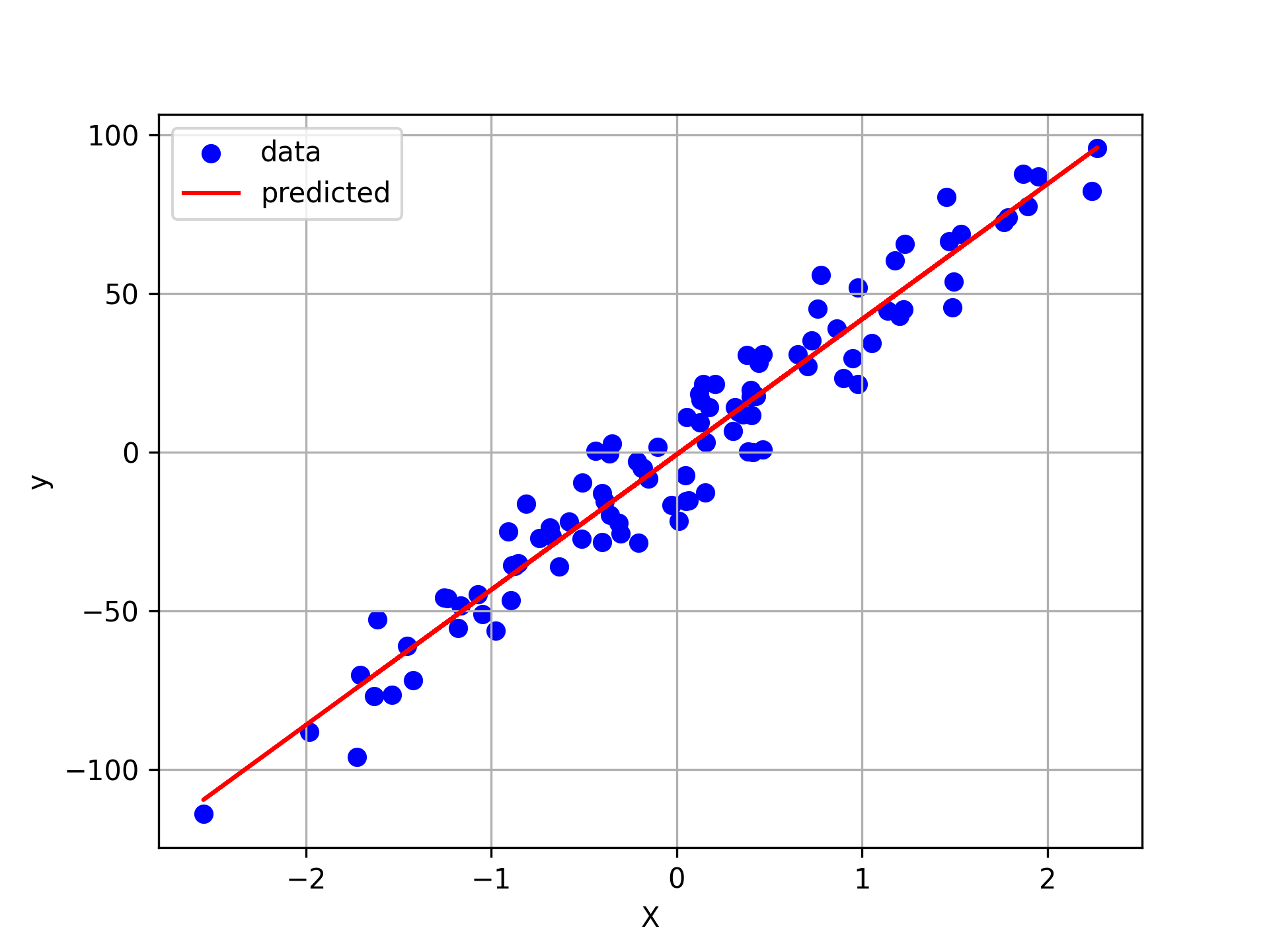
- Regression: Predicting continuous values (e.g., predicting rent prices based on apartment size).
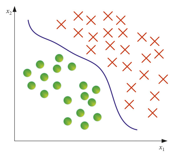
- Classification: Assigning inputs to discrete categories (e.g., diagnosing cancer as benign or malignant).
Example: Regression
- Scenario: Predicting rent prices based on apartment size (in m²).
- Details:
- Input features (X): Apartment size, number of rooms, neighborhood, etc.
- Target variable (Y): Rent price (e.g., $ per month).
- Model’s Job: Learn the relationship between apartment features and rent prices, then predict the rent for a new apartment.
Example: Classification
- Scenario: Diagnosing cancer (e.g., benign or malignant tumor).
- Details:
- Input features (X): Measurements like tumor size, texture, cell shape, etc.
- Target variable (Y): Class label (e.g., “Benign” or “Malignant”).
- Model’s Job: Classify a new tumor as benign or malignant based on input features.
Unsupervised Learning
Unsupervised learning deals with unlabeled data. The model tries to find patterns, structures, or relationships within the data without any predefined labels or targets. It’s often used for exploratory data analysis.
Key Characteristics
- Input Only: The data contains only input features (X), with no target labels (Y).
- Goal: Discover hidden patterns or groupings in the data.
Subfields
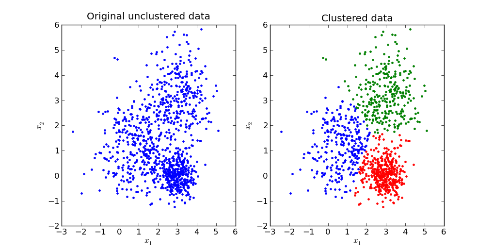
- Clustering: Grouping similar data points into clusters (e.g., customer segmentation).
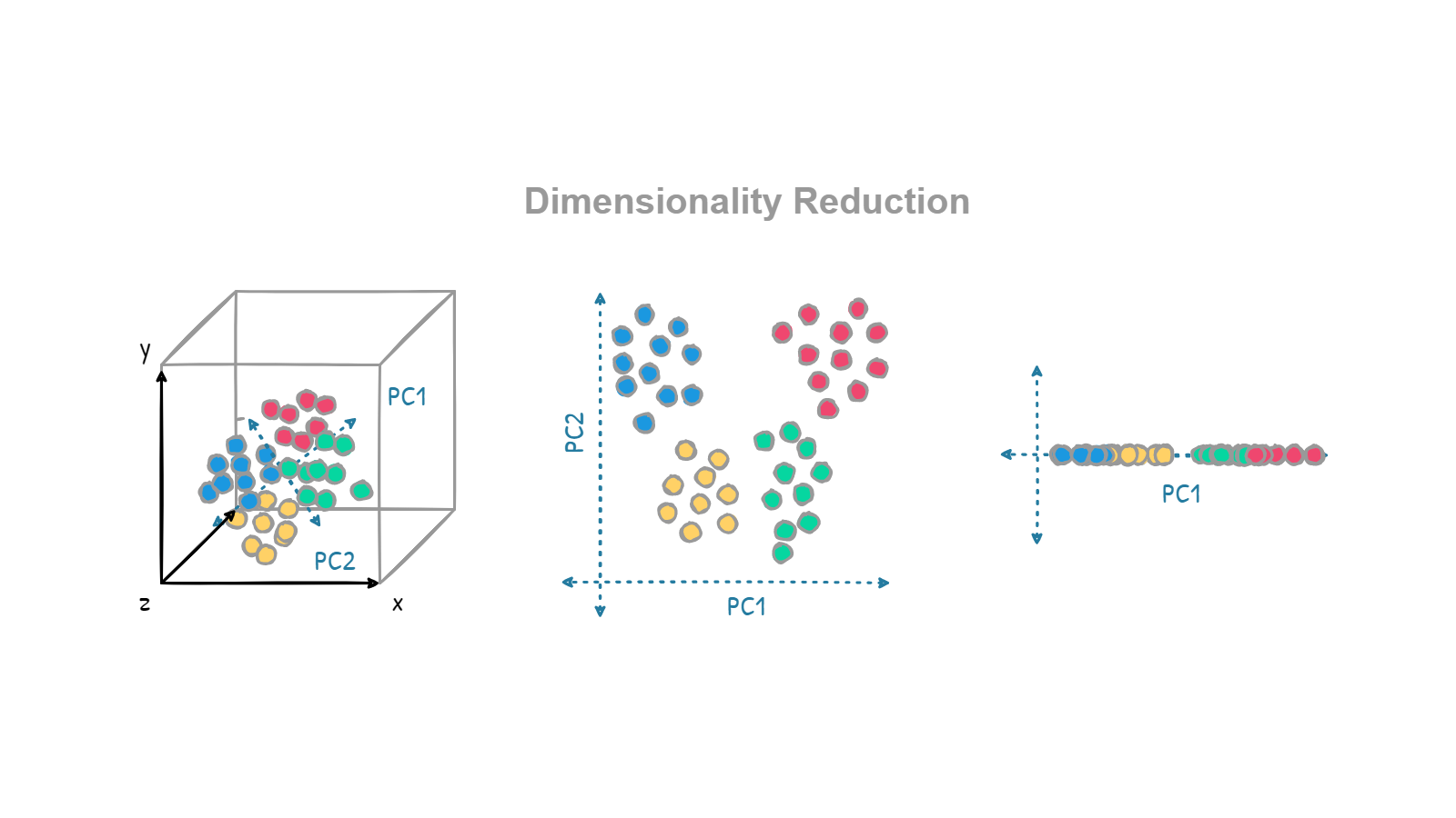
- Dimensionality Reduction: Reducing the number of features in the dataset while preserving important information (e.g., PCA).
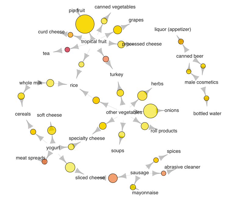
- Association: Discovering relationships or associations between variables in large datasets (e.g., market basket analysis).
Example: Clustering
- Scenario: Grouping customers for targeted marketing.
- Details:
- Input features (X): Customer age, income, purchase history, location, etc.
- No predefined labels (Y).
- Model’s Job: Identify clusters of customers (e.g., “High-spenders,” “Budget-conscious buyers”).
Example: Dimensionality Reduction
- Scenario: Visualizing high-dimensional data.
- Details:
- Imagine you have a dataset with 100+ features (e.g., sensor data from a factory).
- Dimensionality reduction (e.g., PCA) helps reduce it to 2D or 3D for easier visualization.
- Model’s Job: Keep the important structure of the data while reducing complexity.
Example: Association
- Scenario: Market basket analysis to identify product associations.
- Details:
- Input features (X): Transaction data showing items purchased together.
- No predefined labels (Y).
- Model’s Job: Identify rules like “If a customer buys bread, they are likely to buy butter.”
- Use Case: Recommendation systems, inventory planning.
Comparison Table
| Feature | Supervised Learning | Unsupervised Learning |
|---|---|---|
| Data Type | Labeled data (X, Y) | Unlabeled data (X only) |
| Goal | Predict outcomes | Find patterns or structures |
| Key Techniques | Regression, Classification | Clustering, Dimensionality Reduction, Assocation |
| Examples | Fraud detection, Stock price prediction | Market segmentation, Image compression |
Key Takeaways
- Supervised Learning requires labeled data and is commonly used for prediction tasks like regression and classification.
- Unsupervised Learning works with unlabeled data and focuses on finding hidden patterns through clustering or dimensionality reduction.
- Each technique has specific applications and is chosen based on the problem and the data available.
- Linear Regression and Cost Function
Linear Regression and Cost Function
1. Introduction
Linear regression is one of the fundamental algorithms in machine learning. It is widely used for predictive modeling, especially when the relationship between the input and output variables is assumed to be linear. The primary goal is to find the best-fitting line that minimizes the error between predicted values and actual values.
Why Linear Regression?
Linear regression is simple yet powerful for many real-world applications. Some common use cases include:
- Predicting house prices based on features like size, number of rooms, and location.
- Estimating salaries based on experience, education level, and industry.
- Understanding trends in various fields like finance, healthcare, and economics.
Real-World Example: Housing Prices
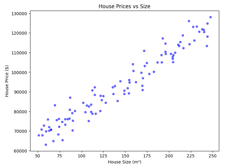
Consider predicting house prices based on the size of the house (in square meters). A simple linear relationship can be assumed: larger houses tend to have higher prices. This assumption is the foundation of our linear regression model.
2. Mathematical Representation
A simple linear regression model assumes a linear relationship between the input $x$ (house size in square meters) and the output $y$ (house price). It is represented as:
$$ h_θ(x) = \theta_0 + \theta_1 x $$
where:
- $h_θ(x) $ is the predicted house price.
- $ \theta_0 $ (intercept) and $\theta_1 $ (slope) are the parameters of the model.
- $x$ is the house size.
- $y$ is the actual house price.
2.1 Understanding the Linear Model
But what does this equation really mean?
-
$\theta_0$ (intercept): The price of a house when its size is 0 m².
-
$\theta_1$ (slope): The increase in house price for every additional square meter.
For example, if:
-
$\theta_0 = 50,000$ and $\theta_1 = 300$,
-
A 100 m² house would cost: $ h_θ(100) = 50000 + 300 \cdot 100 = 80000 $
-
A 200 m² house would cost: $ h_θ(200) = 50000 + 300 \cdot 200 = 110000 $
We can visualize this relationship using a regression line.
3. Implementing Linear Regression Step by Step
To make the theoretical concepts clearer, let’s implement the regression model step by step using Python.
3.1 Import Necessary Libraries
import numpy as np
import matplotlib.pyplot as plt
import seaborn as sns
3.2 Generate Sample Data
np.random.seed(42)
x = 50 + 200 * np.random.rand(100, 1) # House sizes in m² (50 to 250)
y = 50000 + 300 * x + np.random.randn(100, 1) * 5000 # House prices with noise
Here, we create a dataset with 100 samples, where:
-
$x$ represents house sizes (random values between $50$ and $250$ m²).
-
$y$ represents house prices, following a linear relation but with some noise.
3.3 Visualizing the Data
plt.figure(figsize=(8,6))
sns.scatterplot(x=x.flatten(), y=y.flatten(), color='blue', alpha=0.6)
plt.xlabel('House Size (m²)')
plt.ylabel('House Price ($)')
plt.title('House Prices vs Size')
plt.show()
3.4 Plotting the Regression Line
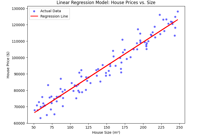
Before moving to cost function, let’s fit a simple regression line to our data and visualize it.
In real-world applications, we don’t manually compute these parameters. Instead, we use libraries like scikit-learn to perform linear regression efficiently.
3.4.1 Compute the Slope ($\theta_1$)
theta_1 = np.sum((x - np.mean(x)) * (y - np.mean(y))) / np.sum((x - np.mean(x))**2)
Here, we compute the slope ($\theta_1$) using the least squares method.
3.4.2 Compute the Intercept ($\theta_0$)
theta_0 = np.mean(y) - theta_1 * np.mean(x)
This calculates the intercept ($\theta_0$), ensuring that our regression line passes through the mean of the data.
3.5 Plotting the Regression Line
y_pred = theta_0 + theta_1 * x # Compute predicted values
plt.figure(figsize=(8,6))
sns.scatterplot(x=x.flatten(), y=y.flatten(), color='blue', alpha=0.6, label='Actual Data')
plt.plot(x, y_pred, color='red', linewidth=2, label='Regression Line')
plt.xlabel('House Size (m²)')
plt.ylabel('House Price ($)')
plt.title('Linear Regression Model: House Prices vs. Size')
plt.legend()
plt.show()
3.6 Interpretation of the Regression Line
Now, what does this line tell us?
✅ If the slope $\theta_1$ is positive, then larger houses cost more (as expected).
✅ If the intercept $\theta_0$ is high, it means even the smallest houses have a significant base price.
✅ The steepness of the line shows how much price increases per square meter.
4. Cost Function
To measure how well our model is performing, we use the cost function. The most common cost function for linear regression is the Mean Squared Error (MSE):
$$ J(\theta) = \frac{1}{2m} \sum (h_{\theta}(x_i) - y_i)^2 $$
where:
- $ m $ is the number of training examples.
- $ h_\theta(x_i) $ is the predicted price for the $ i-th$ house.
- $ y_i $ is the actual price.
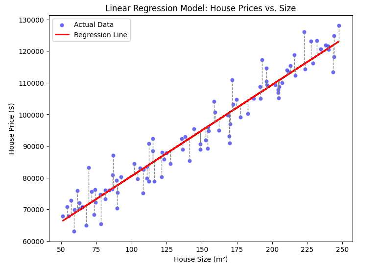
Any dashed line indicates an error. In the formula above, we calculated the sum of these, namely $J(\theta)$.
This function calculates the average squared difference between predicted and actual values, penalizing larger errors more. The goal is to minimize $J(\theta)$ to achieve the best model parameters.
4.1 Example: Assuming $\theta_1 = 0$
To illustrate how the cost function behaves, let’s assume that $\theta_1 = 0$, meaning our model only depends on $\theta_0$. We’ll use a small dataset with four x values and y values:
| x values | y values |
|---|---|
| 1 | 2 |
| 2 | 4 |
| 3 | 6 |
| 4 | 8 |
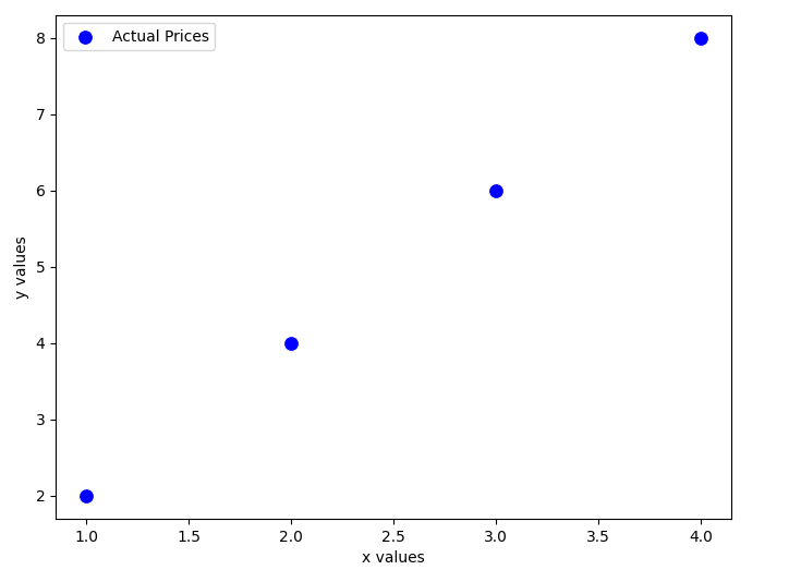
Since we assume $\theta_1 = 0$, our hypothesis function simplifies to: $$h_{\theta}(x) = \theta_0 \cdot x $$
We’ll evaluate different values of $\theta_0$ and compute the corresponding cost function.
Case 1: $\theta_0 = 1$
For $\theta_0 = 1$, the predicted values are:
$$ h_θ(x) = 1 \cdot x = [1, 2, 3, 4] $$
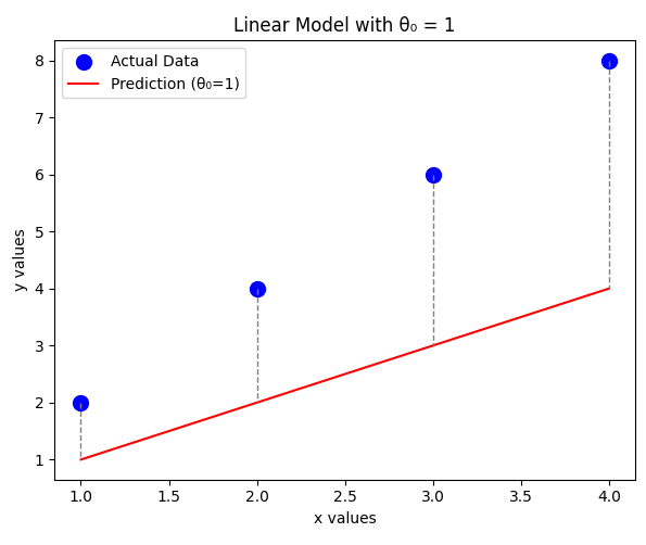
The error values:
$$ \text{error} = h_θ(x) - y = [1 - 2, 2 - 4, 3 - 6, 4 - 8] = [-1, -2, -3, -4] $$
Computing the cost function:
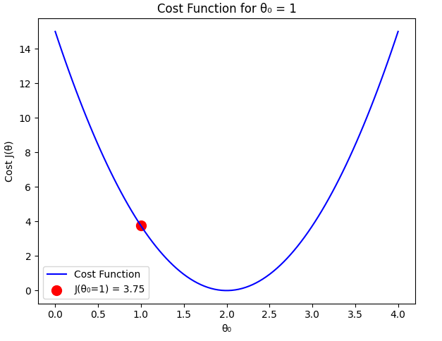
$$ J(\theta0 = 1) = \frac{1}{2m} \sum (h{\theta}(x_i) - y_i)^2 $$
$$ J(1) = \frac{1}{8} ((-1)^2 + (-2)^2 + (-3)^2 + (-4)^2) = \frac{1}{8} (1 + 4 + 9 + 16) = \frac{30}{8} = 3.75 $$
Case 2: $\theta_0 = 1.5$
For $\theta_0 = 1.5$, the predicted values are:
$$ h_θ(x) = 1.5 \cdot x = [1.5, 3, 4.5, 6] $$
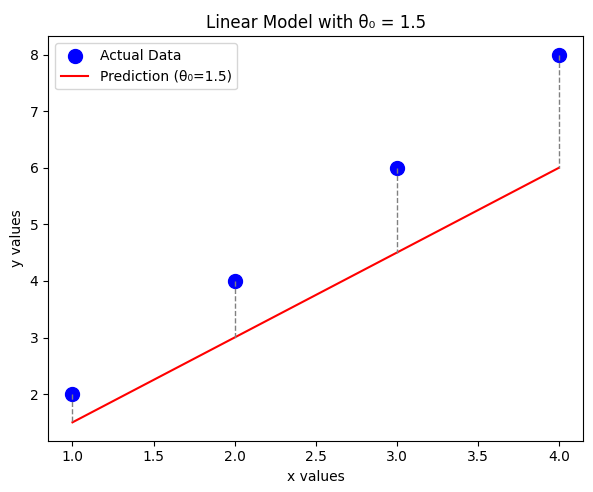
The error values:
$$ \text{error} = [1.5 - 2, 3 - 4, 4.5 - 6, 6 - 8] = [-0.5, -1, -1.5, -2] $$
Computing the cost function:
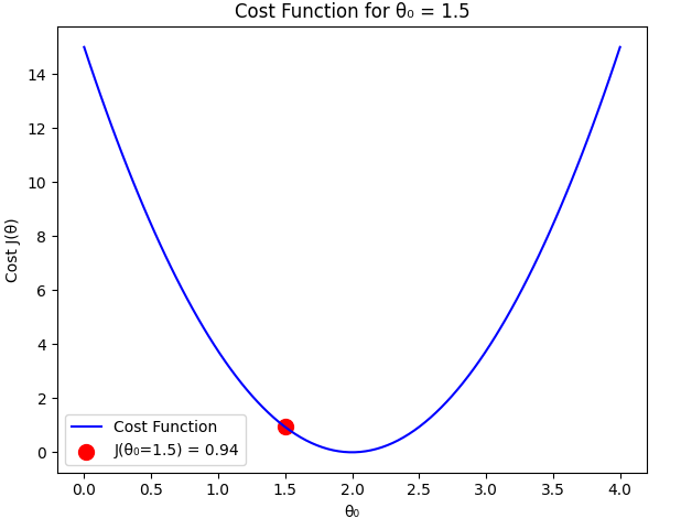
$$ J(1.5) = \frac{1}{8} ((-0.5)^2 + (-1)^2 + (-1.5)^2 + (-2)^2) $$
$$ J(1.5) = \frac{1}{8} (0.25 + 1 + 2.25 + 4) = \frac{7.5}{8} = 0.9375 $$
Case 3: $\theta_0 = 2$ (Optimal Case)
For $\theta_0 = 2$, the predicted values match the actual values:
$$ h_θ(x) = 2 \cdot x = [2, 4, 6, 8] $$
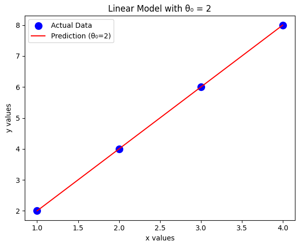
The error values:
$$ \text{error} = [2 - 2, 4 - 4, 6 - 6, 8 - 8] = [0, 0, 0, 0] $$
Computing the cost function:
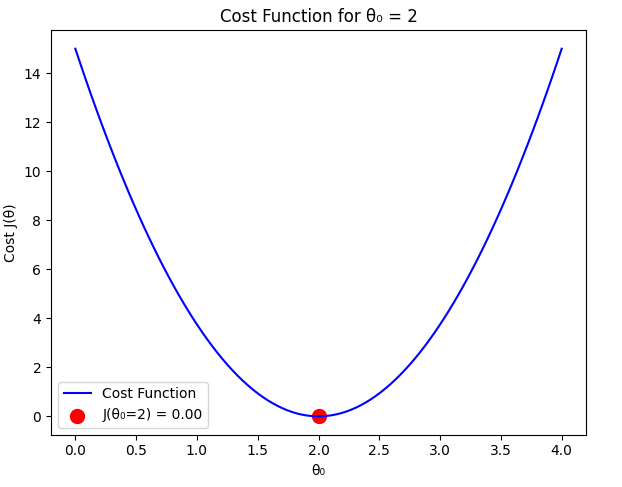
$$ J(2) = \frac{1}{8} ((0)^2 + (0)^2 + (0)^2 + (0)^2) = 0 $$
Comparison
From our calculations:
- $ J(1) = 3.75 $
- $ J(1.5) = 0.9375 $
- $ J(2) = 0 $
As expected, the cost function is minimized when $\theta_0 = 2$, which perfectly fits the dataset. Any deviation from this value results in a higher cost.
So how many times can the machine try and find the correct value? How can we teach it this? The answer is in the next topic.
Gradient Descent
- Introduction to Gradient Descent
- Mathematical Formulation of Gradient Descent
- Learning Rate ($\alpha$)
- Gradient Descent Convergence
- Local Minimum vs Global Minimum
Introduction to Gradient Descent
In the previous section, we explored how the cost function behaves when assuming different values of $\theta_0$ with $\theta_1 = 0$ (To visualize it easily, we give zero to $\theta_1$). Now, we introduce Gradient Descent, an optimization algorithm used to find the best parameters that minimize the cost function $J(\theta)$.
our hypothesis function simplifies to: $$h_{\theta}(x) = \theta_0 \cdot x $$
Gradient Descent is an iterative method that updates the parameter $\theta$ step by step in the direction that reduces the cost function. The algorithm helps us find the optimal value of $\theta_0$ efficiently instead of manually testing different values.
To understand how Gradient Descent works, let’s recall our dataset:
| x values | y values |
|---|---|
| 1 | 2 |
| 2 | 4 |
| 3 | 6 |
| 4 | 8 |
We aim to find the best value of $\theta_0$ that minimizes the error between our predictions $h_\theta(x) = \theta_0 \cdot x$ and the actual $y$ values. Gradient Descent will iteratively adjust $\theta_0$ to reach the minimum cost.
Mathematical Formulation of Gradient Descent
Gradient Descent is an optimization algorithm used to minimize a function by iteratively updating its parameters in the direction of the steepest descent. In our case, we aim to minimize the cost function:
$$ J(\theta) = \frac{1}{2m} \sum (h_θ(x_i) - y_i)^2 $$
Where:
- 𝑚 is the number of training examples.
- $h_θ(x)$ represents our hypothesis function (predicted values).
- y represents the actual target values.
- Goal: Find the optimal $θ$ that minimizes $J(θ)$.
1. Gradient Descent Update Rule
Gradient Descent uses the derivative of the cost function to determine the direction and magnitude of updates. The general update rule for $\theta$ is:
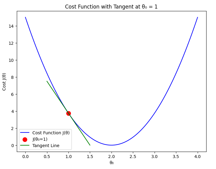
$$\theta := \theta - \alpha \frac{\partial J(\theta)}{\partial \theta}$$
Where:
- $\alpha$ (learning rate) controls the step size of updates.
- $\frac{\partial J(\theta)}{\partial \theta} $ is the gradient (derivative) of the cost function with respect to $ \theta $.
Why Do We Use the Derivative?
The derivative $\frac{\partial J(\theta)}{\partial \theta} $ tells us the slope of the cost function. If the slope is positive, we need to decrease $θ_0$ , and if it is negative, we need to increase $θ_0$, guiding us toward the minimum of $J(θ_0)$ . Without derivatives, we wouldn’t know which direction to move to minimize the function.
The gradient tells us how steeply the function increases or decreases at a given point.
- If the gradient is positive, $ \theta $ is decreased.
- If the gradient is negative, $ \theta $ is increased.
This ensures that we move toward the minimum of the cost function.
2. Computing the Gradient
First, recall our hypothesis function:
$$ h_θ(x) = \theta_0 \cdot x $$
Now, we compute the derivative of the cost function:
$$ \frac{\partial J(\theta)}{\partial \theta*0} = \frac{1}{m} \sum (h_θ(x^{(i)}) - y^{(i)}) x^{(i)} $$
This expression represents the average gradient of the errors multiplied by the input values. Using this gradient, we update $ \theta_0 $ in each iteration:
$$ \theta*0 := \theta_0 - \alpha \cdot \frac{1}{m} \sum(h_θ(x^{(i)}) - y^{(i)}) x^{(i)} $$
- If the error is large, the update step is bigger.
- If the error is small, the update step is smaller.
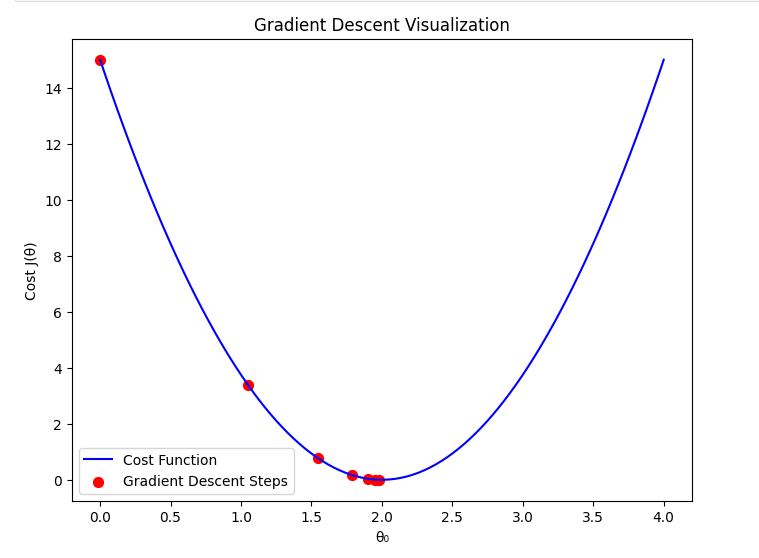
This way, the algorithm gradually moves towards the optimal $ \theta_0 $.
Learning Rate ($\alpha$)
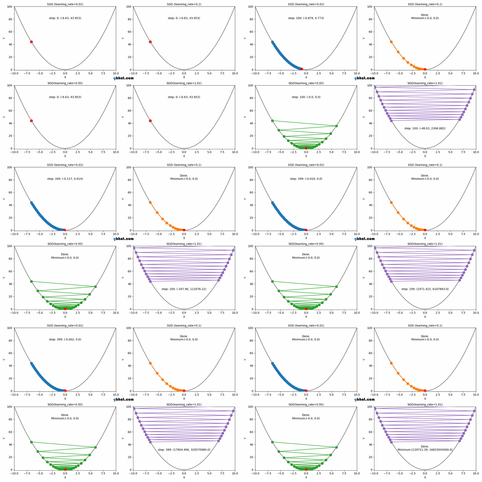
The learning rate $(\alpha)$ is a crucial parameter in the gradient descent algorithm. It determines how large a step we take in the direction of the negative gradient during each iteration. Choosing an appropriate learning rate is essential for ensuring efficient convergence of the algorithm.
If the learning rate is too small, the algorithm will take tiny steps towards the minimum, leading to slow convergence. On the other hand, if the learning rate is too large, the algorithm may overshoot the minimum or even diverge, never reaching an optimal solution.
1. When $\alpha$ is Too Small
If the learning rate is set too small:
- Gradient descent will take very small steps in each iteration.
- Convergence to the minimum cost will be extremely slow.
- It may take a large number of iterations to reach a useful solution.
- The algorithm might get stuck in local variations of the cost function, slowing down learning.
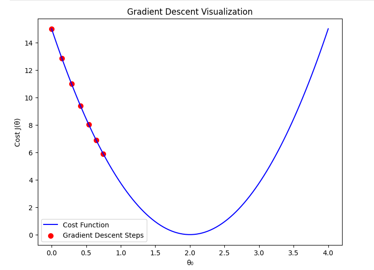
Mathematically, the update rule is: $\theta_0 := \theta_0 - \alpha \frac{d}{d\theta_0} J(\theta_0) $ When $\alpha$ is very small, the change in $\theta_0$ per step is minimal, making the process inefficient.
2. When $\alpha$ is Optimal
If the learning rate is chosen optimally:
- The gradient descent algorithm moves efficiently towards the minimum.
- It balances speed and stability, converging in a reasonable number of iterations.
- The cost function decreases steadily without oscillations or divergence.
A well-chosen $\alpha$ ensures that gradient descent follows a smooth and steady path to the minimum.
3. When $\alpha$ is Too Large
If the learning rate is set too large:
- Gradient descent may take excessively large steps.
- Instead of converging, it may oscillate around the minimum or diverge entirely.
- The cost function might increase instead of decreasing due to overshooting the optimal $\theta_0$.
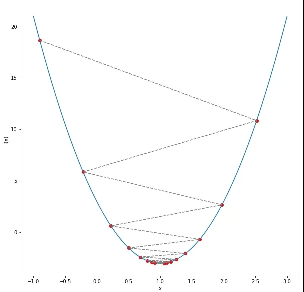
In extreme cases, the cost function values might increase indefinitely, causing the algorithm to fail to find a minimum.
Summary
Selecting the right learning rate is essential for gradient descent to work efficiently. A well-balanced $\alpha$ ensures that the algorithm converges quickly and effectively. In the next section, we will implement gradient descent with different learning rates to visualize their effects.
Gradient Descent Convergence
Gradient Descent is an iterative optimization algorithm that minimizes the cost function, J(\theta), by updating parameters step by step. However, we need a proper stopping criterion to determine when the algorithm has converged.
1. Convergence Criteria
The algorithm should stop when one of the following conditions is met:
- Small Gradient: If the derivative (gradient) of the cost function is close to zero, meaning the algorithm is near the optimal point.
- Minimal Cost Change: If the difference in the cost function between iterations is below a predefined threshold ($ |J(\thetat) - J(\theta{t-1})| < \varepsilon $).
- Maximum Iterations: A fixed number of iterations is reached to avoid infinite loops.
2. Choosing the Right Stopping Condition
- Stopping Too Early: If the algorithm stops before reaching the optimal solution, the model may not perform well.
- Stopping Too Late: Running too many iterations may waste computational resources without significant improvement.
- Optimal Stopping: The best condition is when further updates do not significantly change the cost function or parameters.
Local Minimum vs Global Minimum
Understanding the Concept
When optimizing a function, we aim to find the point where the function reaches its lowest value. This is crucial in machine learning because we want to minimize the cost function $ J(\theta) $ effectively. However, there are two types of minima that gradient descent might encounter:
- Global Minimum: The absolute lowest point of the function. Ideally, gradient descent should converge here.
- Local Minimum: A point where the function has a lower value than nearby points but is not the absolute lowest value.
For convex functions (such as our quadratic cost function), gradient descent is guaranteed to reach the global minimum. However, for non-convex functions, the algorithm may get stuck in a local minimum.
Convex vs Non-Convex Cost Functions
- Convex Functions
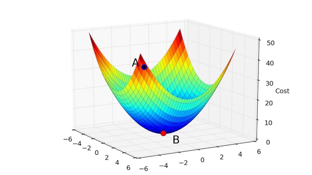
- The cost function $ J(\theta) $ is convex for linear regression.
- This ensures that gradient descent always leads to the global minimum.
- Example: A simple quadratic function like $ J(\theta) = (\theta - 2)^2 $.
- Non-Convex Functions
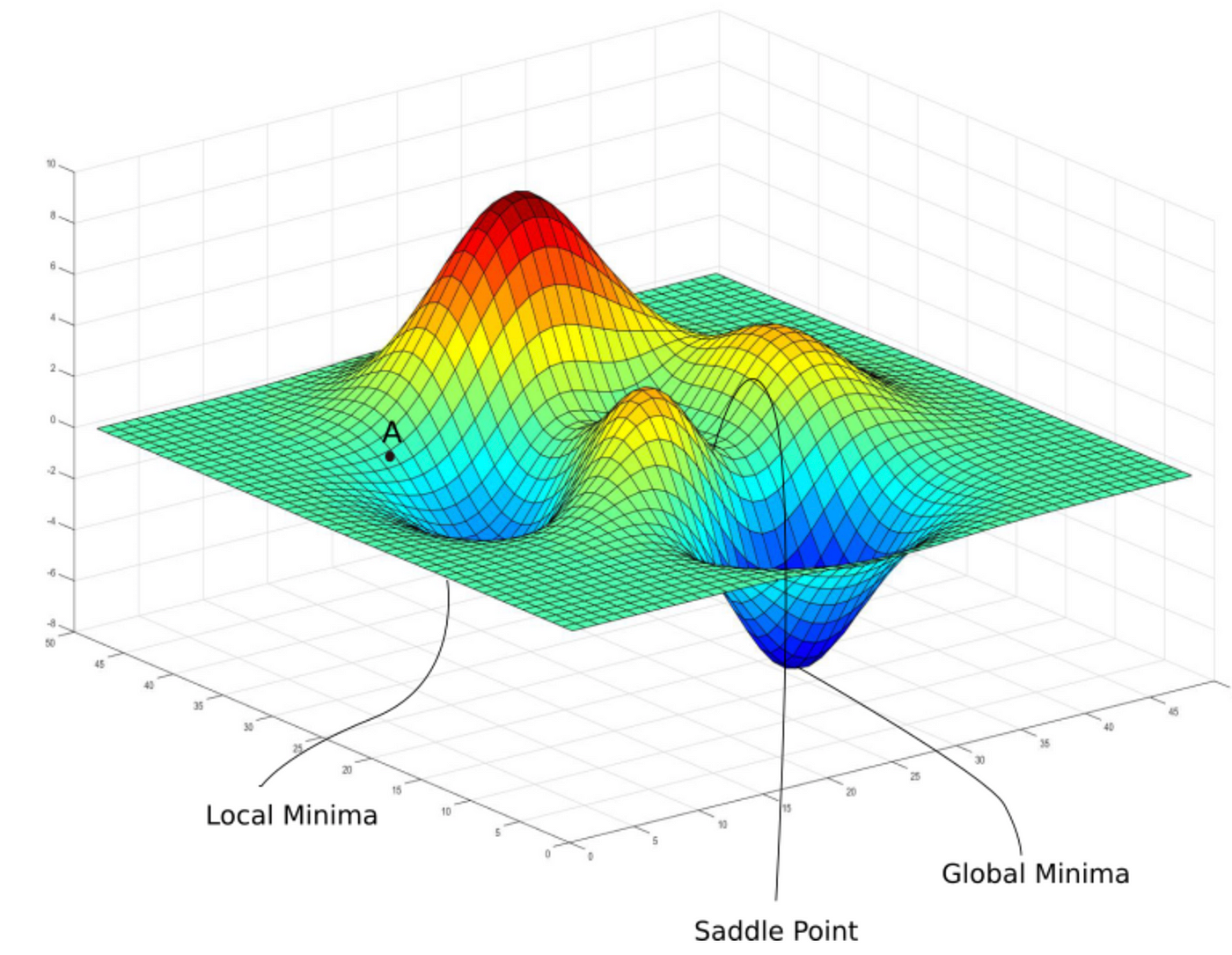
- More common in deep learning and complex machine learning models.
- There can be multiple local minima.
- Example: Functions with multiple peaks and valleys, such as $J(\theta) = \sin(\theta) + \frac{\theta^2}{10} $.
Multiple Features
Introduction
In real-world scenarios, a single feature is often not enough to make accurate predictions. For example, if we want to predict the price of a house, using only its size (square meters) might not be sufficient. Other factors such as the number of bedrooms, location, and age of the house also play an important role.
When we have multiple features, our hypothesis function extends to:
$$ h_{\theta}(x) = \theta_0 + \theta_1 x_1 + \theta_2 x_2 + … + \theta_n x_n $$
where:
- $ x_1, x_2, …, x_n $ are the input features,
- $ \theta_0, \theta_1, …, \theta_n $ are the parameters (weights) we need to learn.
For instance, in a house price prediction model, the hypothesis function could be:
$$ h_{\theta}(x) = \theta_0 + \theta_1 (\text{Size}) + \theta_2 (\text{Number of Bedrooms}) + \theta_3 (\text{Age of House}) $$
This allows our model to consider multiple factors, improving its accuracy compared to using a single feature.
Vectorization
To optimize computations, we represent our hypothesis function using matrix notation:
where:
$ X $ is the matrix containing training examples
$ \theta $ is the parameter vector
This allows efficient computation using matrix operations instead of looping over individual training examples.
Why Vectorization?
Vectorization is the process of converting operations that use loops into matrix operations. This improves computational efficiency, especially when working with large datasets. Instead of computing predictions one by one using a loop, we leverage linear algebra to perform all calculations simultaneously.
Without vectorization (using a loop):
m = len(X) # Number of training examples
h = []
for i in range(m):
prediction = theta_0 + theta_1 * X[i, 1] + theta_2 * X[i, 2] + ... + theta_n * X[i, n]
h.append(prediction)
With vectorization:
h = np.dot(X, theta) # Compute all predictions at once
This method is significantly faster because it takes advantage of optimized numerical libraries like NumPy that execute matrix operations efficiently.
Vectorized Cost Function
Similarly, our cost function for multiple features is:
$$ J(\theta) = \frac{1}{2m} \sum(h_θ(x^{(i)}) - y^{(i)})^2 $$
Using matrices, this can be written as:
$$ J(\theta) = \frac{1}{2m} (X\theta - y)^T (X\theta - y) $$
And implemented in Python as:
def compute_cost(X, y, theta):
m = len(y) # Number of training examples
error = np.dot(X, theta) - y # Compute (Xθ - y)
cost = (1 / (2 * m)) * np.dot(error.T, error) # Compute cost function
return cost
By using vectorized operations, we achieve a significant performance boost compared to using explicit loops.
Feature Scaling
When working with multiple features, the range of values across different features can vary significantly. This can negatively affect the performance of gradient descent, causing slow convergence or inefficient updates. Feature scaling is a technique used to normalize or standardize features to bring them to a similar scale, improving the efficiency of gradient descent.
Why Feature Scaling is Important
- Features with large values can dominate the cost function, leading to inefficient updates.
- Gradient descent converges faster when features are on a similar scale.
- Helps prevent numerical instability when computing gradients.
Methods of Feature Scaling
1. Min-Max Scaling (Normalization)
Brings all feature values into a fixed range, typically between 0 and 1:
$$x^{(i)}{scaled} = \frac{x^{(i)} - x{min}}{x_{max} - x_{min}}$$
- Best for cases where the distribution of data is not Gaussian.
- Sensitive to outliers, as extreme values affect the range.
2. Standardization (Z-Score Normalization)
Centers data around zero with unit variance:
$$x^{(i)}_{scaled} = \frac{x^{(i)} - \mu}{\sigma}$$
where:
-
$ \mu $ is the mean of the feature values
-
$ \sigma $ is the standard deviation
-
Works well when features follow a normal distribution.
-
Less sensitive to outliers compared to min-max scaling.
Example
Consider a dataset with two features: House Size (m²) and Number of Bedrooms.
| House Size (m²) | Bedrooms |
|---|---|
| 2100 | 3 |
| 1600 | 2 |
| 2500 | 4 |
| 1800 | 3 |
Using min-max scaling:
| House Size (scaled) | Bedrooms (scaled) |
|---|---|
| 0.714 | 0.5 |
| 0.0 | 0.0 |
| 1.0 | 1.0 |
| 0.286 | 0.5 |
Feature Scaling in Gradient Descent
After scaling, gradient descent updates will be more balanced across different features, leading to faster and more stable convergence. Feature scaling is a critical preprocessing step in machine learning models involving optimization algorithms like gradient descent.
Feature Engineering and Polynomial Regression
- Feature Engineering
- Polynomial Regression
Feature Engineering
Introduction to Feature Engineering
Feature engineering is the process of transforming raw data into meaningful features that improve the predictive power of machine learning models. It involves creating new features, modifying existing ones, and selecting the most relevant features to enhance model performance.
Why is Feature Engineering Important?
- Improves model accuracy: Well-engineered features help models learn better representations of the data.
- Reduces model complexity: Properly engineered features can make complex models simpler and more interpretable.
- Enhances generalization: Good feature selection prevents overfitting and improves performance on unseen data.
Real-World Example
Consider a house price prediction problem. Instead of using just raw data such as square footage and the number of bedrooms, we can create new features like:
- Price per square foot =
Price / Size - Age of the house =
Current Year - Year Built - Proximity to city center =
Distance in km
These engineered features often provide better insights and improve model performance compared to using raw data alone.
Feature Transformation
Feature transformation involves applying mathematical operations to existing features to make data more suitable for machine learning models.
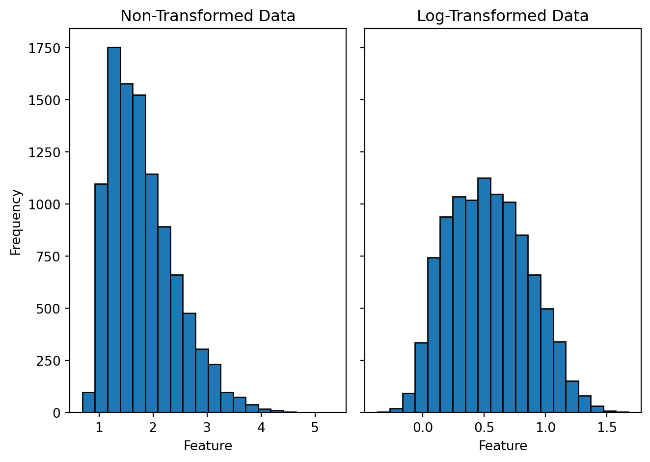
1. Log Transformation
Used to reduce skewness and stabilize variance in highly skewed data.
Example: Income Data
Many income datasets have a right-skewed distribution where most values are low, but a few values are extremely high. Applying a log transformation makes the data more normal:
$$X’ = \log(X)$$
2. Polynomial Features
Adding polynomial terms (squared, cubic) to capture non-linear relationships.
Example: House Price Prediction
Instead of using Size as a single feature, we can include Size^2 and Size^3 to better fit non-linear patterns.
from sklearn.preprocessing import PolynomialFeatures
import numpy as np
X = np.array([[1000], [1500], [2000], [2500]]) # House sizes
poly = PolynomialFeatures(degree=2)
X_poly = poly.fit_transform(X)
print(X_poly)
3. Interaction Features
Creating new features based on interactions between existing ones.
Example: Combining Features
Instead of using Height and Weight separately for a health model, create a new BMI feature:
$$BMI = \frac{Weight}{Height^2}$$
def calculate_bmi(height, weight):
return weight / (height ** 2)
height = np.array([1.65, 1.75, 1.80]) # Heights in meters
weight = np.array([65, 80, 90]) # Weights in kg
bmi = calculate_bmi(height, weight)
print(bmi)
This allows the model to understand health risks better than using height and weight separately.
Feature Selection
Feature selection involves identifying the most relevant features for a model while removing unnecessary or redundant ones. This improves model performance and reduces computational complexity.
1. Unnecessary Features
Not all features contribute equally to model performance. Some may be irrelevant or redundant, leading to overfitting and increased computational cost. Examples of unnecessary features include:
- ID columns: Unique identifiers that do not provide predictive value.
- Highly correlated features: Features that contain similar information.
- Constant or near-constant features: Features with little to no variation.
2. Correlation Analysis
Correlation analysis helps detect multicollinearity, where two or more features are highly correlated. If two features provide similar information, one of them can be removed.
Example: Finding Highly Correlated Features
import pandas as pd
import numpy as np
# Sample dataset
data = {
'Feature1': [1, 2, 3, 4, 5],
'Feature2': [2, 4, 6, 8, 10],
'Feature3': [5, 3, 6, 9, 2]
}
df = pd.DataFrame(data)
# Compute correlation matrix
correlation_matrix = df.corr()
print(correlation_matrix)
Features with a correlation coefficient close to ±1 can be considered redundant and removed.
3. Statistical Feature Selection Methods
Feature selection techniques can be used to rank the importance of different features based on statistical tests or model-based importance measures.
At this stage it is enough to learn superficially !
Common Methods:
- Chi-Square Test: Measures dependency between categorical features and the target variable.
- Mutual Information: Evaluates how much information a feature contributes.
- Recursive Feature Elimination (RFE): Iteratively removes less important features based on model performance.
- Feature Importance from Tree-Based Models: Decision trees and random forests provide feature importance scores.
Feature selection ensures that only the most valuable features are used in the final model, improving efficiency and predictive power.
Polynomial Regression
Introduction to Polynomial Regression
Polynomial Regression is an extension of Linear Regression that models non-linear relationships between input features and the target variable. While Linear Regression assumes a straight-line relationship, Polynomial Regression captures curves and more complex patterns.
Why Use Polynomial Regression?
- Handles Non-Linearity: Unlike Linear Regression, which assumes a direct relationship, Polynomial Regression models curved trends.
- Better Fit for Real-World Data: Many real-world phenomena, such as population growth, economic trends, and physics-based models, exhibit non-linear behavior.
- Feature Engineering Alternative: Instead of manually creating interaction terms, Polynomial Regression provides an automatic way to capture complex dependencies.
Example: Predicting House Prices
Consider a dataset where house prices do not increase linearly with size. Instead, they follow a non-linear trend due to factors like demand, location, and infrastructure. A Polynomial Regression model can better capture this pattern.
For instance:
- Linear Model: $ Price = \beta_0 + \beta_1 \cdot Size $
- Polynomial Model: $ Price = \beta_0 + \beta_1 \cdot Size + \beta_2 \cdot Size^2 $
This quadratic term helps model the curved price trend more accurately.
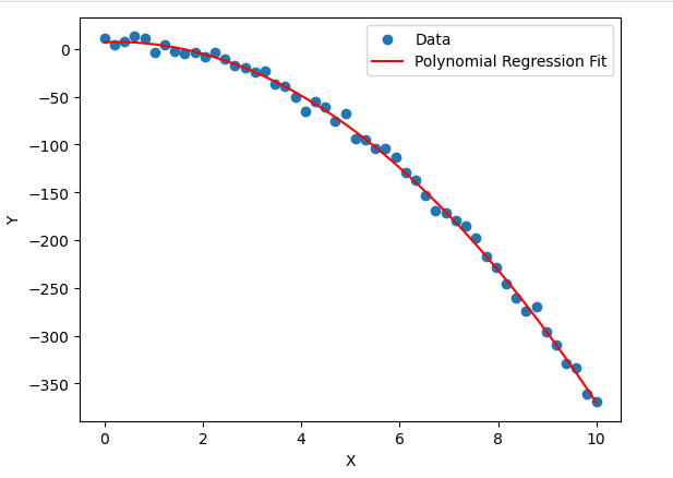
Mathematical Representation and Implementation
Polynomial regression extends linear regression by adding polynomial terms to the feature set. The hypothesis function is represented as:
$$ h_{\theta}(x) = \theta_0 + \theta_1 x + \theta_2 x^2 + \theta_3 x^3 + … + \theta_n x^n $$
where:
- $ x $ is the input feature,
- $ \theta_0, \theta_1, …, \theta_n $ are the parameters (weights),
- $ x^n $ represents higher-degree polynomial terms.
This allows the model to capture non-linear relationships in the data.
Classification with Logistic Regression
- 1. Introduction to Classification
- 2. Logistic Regression
- 3. Cost Function for Logistic Regression
- 4. Gradient Descent for Logistic Regression
1. Introduction to Classification
Classification is a supervised learning problem where the goal is to predict discrete categories instead of continuous values. Unlike regression, which predicts numerical values, classification assigns data points to labels or classes.
Classification vs. Regression
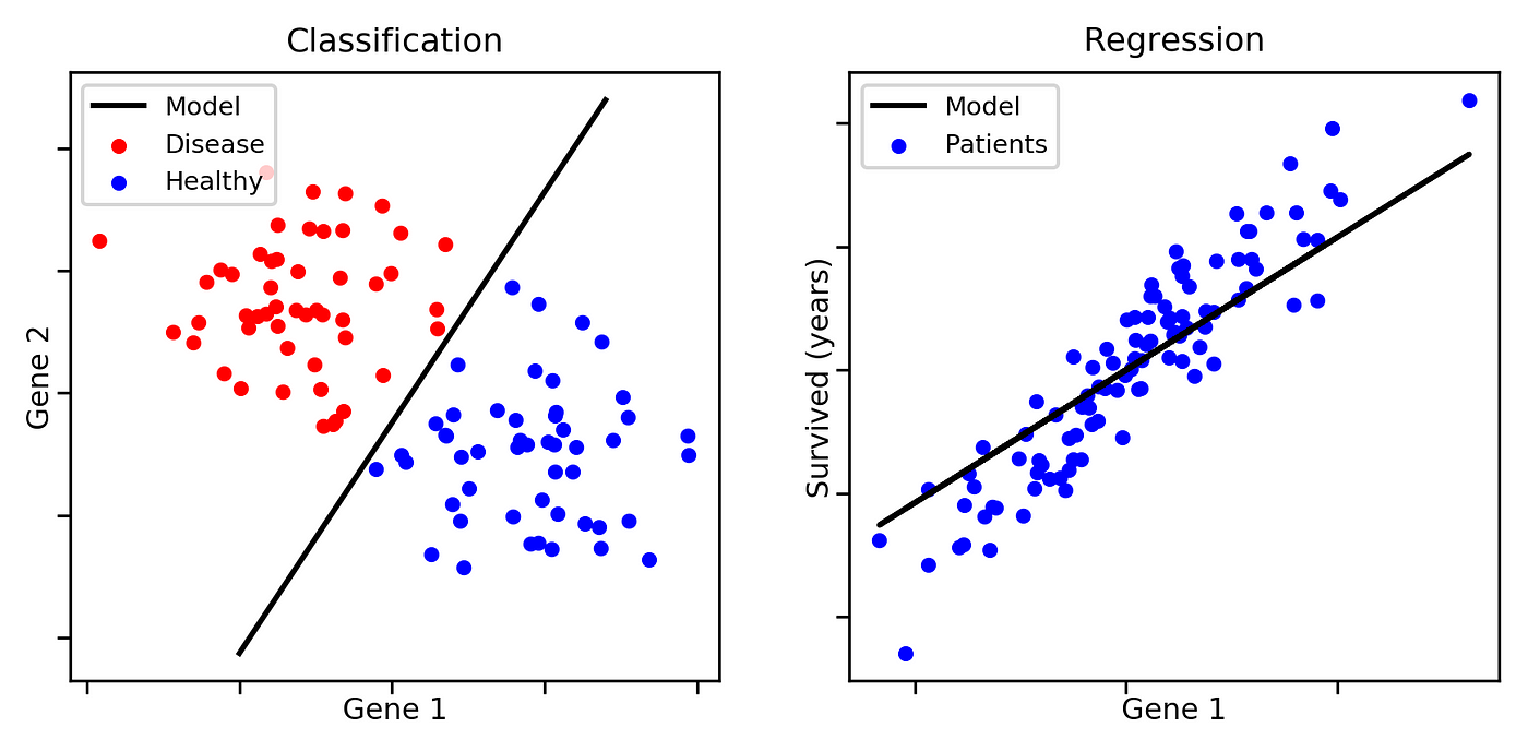
| Feature | Regression | Classification |
|---|---|---|
| Output Type | Continuous | Discrete |
| Example | Predicting house prices | Email spam detection |
| Algorithm Example | Linear Regression | Logistic Regression |
Examples of Classification Problems
- Email Spam Detection: Classify emails as “spam” or “not spam”.
- Medical Diagnosis: Identify whether a patient has a disease (yes/no).
- Credit Card Fraud Detection: Determine if a transaction is fraudulent or legitimate.
- Image Recognition: Classifying images as “cat” or “dog”.
Classification models can be:
- Binary Classification: Only two possible outcomes (e.g., spam or not spam).
- Multi-class Classification: More than two possible outcomes (e.g., classifying handwritten digits 0-9).
2. Logistic Regression
Introduction to Logistic Regression
Logistic regression is a statistical model used for binary classification problems. Unlike linear regression, which predicts continuous values, logistic regression predicts probabilities that map to discrete class labels.
Linear regression might seem like a reasonable approach for classification, but it has major limitations:
- Unbounded Output: Linear regression produces outputs that can take any real value, meaning predictions could be negative or greater than 1, which makes no sense for probability-based classification.
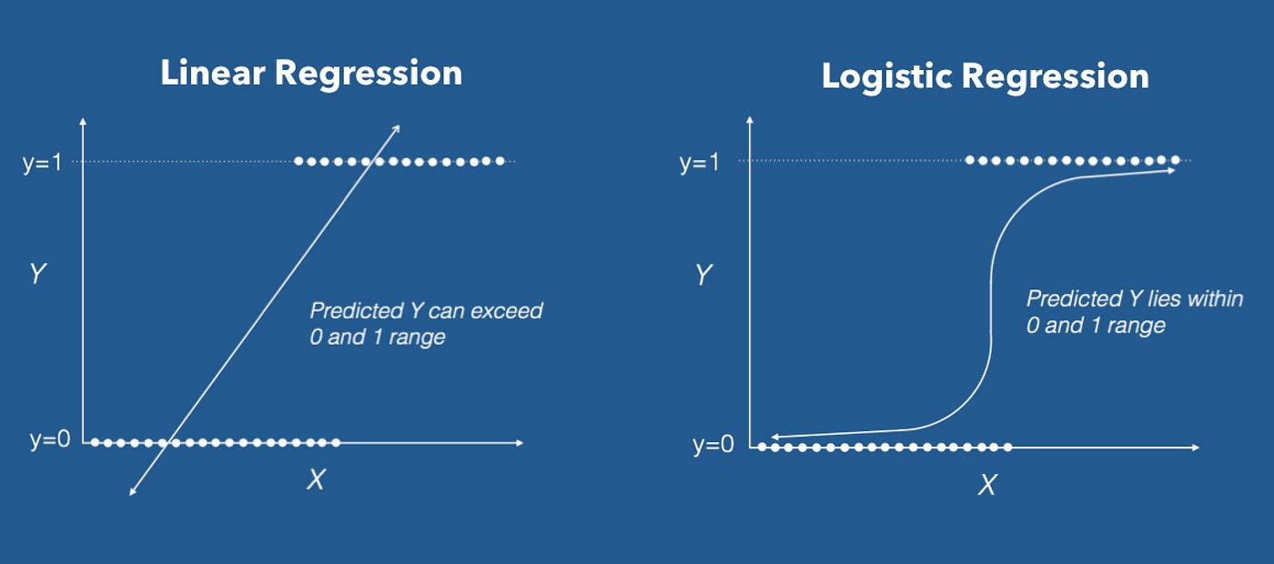
- Poor Decision Boundaries: If we use a linear function for classification, extreme values in the dataset can distort the decision boundary, leading to incorrect classifications.
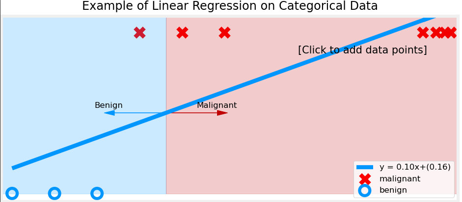
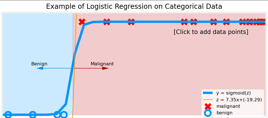
To solve these issues, we use logistic regression, which applies the sigmoid function to transform outputs into a probability range between 0 and 1.
Why Do We Need the Sigmoid Function?
The sigmoid function is a key component of logistic regression. It ensures that outputs always remain between 0 and 1, making them interpretable as probabilities.
Consider a fraud detection system that predicts whether a transaction is fraudulent (1) or legitimate (0) based on customer behavior. Suppose we use a linear model:
$$ y = \theta_0 + \theta_1 x_1 + \theta_2 x_2 $$
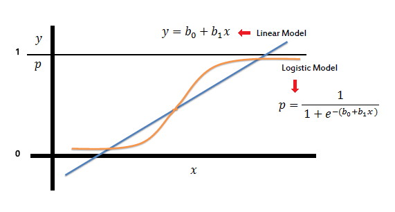
For some transactions, the output might be y = 7.5 or y = -3.2, which do not make sense as probability values. Instead, we use the sigmoid function to squash any real number into a valid probability range:
$$ h_{\theta}(x) = \frac{1}{1 + e^{-\theta^T x}} $$
This function maps:
- Large positive values to probabilities close to 1 (fraudulent transaction).
- Large negative values to probabilities close to 0 (legitimate transaction).
- Values near 0 to probabilities near 0.5 (uncertain classification).
Sigmoid Function and Probability Interpretation
The output of the sigmoid function can be interpreted as:
- $ h_θ(x) \approx 1 $ → The model predicts Class 1 (e.g., spam email, fraudulent transaction).
- $ h_θ(x) \approx 0 $ → The model predicts Class 0 (e.g., not spam email, legitimate transaction).
For a final classification decision, we apply a threshold (typically 0.5):
$$ \hat{y} = \begin{cases} 1, & \text{if } h_{\theta}(x) \geq 0.5 \ 0, & \text{if } h_{\theta}(x) < 0.5 \end{cases} $$
This means:
- If the probability is ≥ 0.5, we classify the input as 1 (positive class).
- If the probability is < 0.5, we classify it as 0 (negative class).
Decision Boundary
The decision boundary is the surface that separates different classes in logistic regression. It is the point at which the model predicts a probability of 0.5, meaning the model is equally uncertain about the classification.
Since logistic regression produces probabilities using the sigmoid function, we define the decision boundary mathematically as:
$$ h_{\theta}(x) = \frac{1}{1 + e^{-\theta^T x}} = 0.5 $$
Taking the inverse of the sigmoid function, we get:
$$ \theta^T x = 0 $$
This equation defines the decision boundary as a linear function in the feature space.
Understanding the Decision Boundary with Examples
1. Single Feature Case (1D)
If we have only one feature $ x_1 $, the model equation is:
$$ \theta_0 + \theta_1 x_1 = 0 $$
Solving for $ x_1 $:
$$ x_1 = -\frac{\theta_0}{\theta_1} $$
This means that when $ x_1 $ crosses this threshold, the model switches from predicting Class 0 to Class 1.
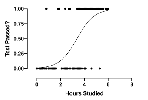
Example: Imagine predicting whether a student passes or fails based on study hours ($ x_1 $):
- If $ x_1 < 5 $ hours → Fail (Class 0).
- If $ x_1 \geq 5 $ hours → Pass (Class 1).
The decision boundary in this case is simply $ x_1 = 5 $.
2. Two Features Case (2D)
For two features $ x_1 $ and $ x_2 $, the decision boundary equation becomes:
$$ \theta_0 + \theta_1 x_1 + \theta_2 x_2 = 0 $$
Rearranging:
$$ x_2 = -\frac{\theta_0}{\theta_2} - \frac{\theta_1}{\theta_2} x_1 $$
This represents a straight line separating the two classes in a 2D plane.
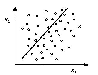
Example: Suppose we classify students as passing (1) or failing (0) based on study hours ($ x_1 $) and sleep hours ($ x_2 $):
- The decision boundary could be: $$ x_2 = -2 - 0.5 x_1 $$
- If $ x_2 $ is above the line, classify as pass.
- If $ x_2 $ is below the line, classify as fail.
3. Two Features Case (3D)
When we move to three features $ x_1 $, $ x_2 $, and $ x_3 $, the decision boundary becomes a plane in three-dimensional space:
$$ \theta_0 + \theta_1 x_1 + \theta_2 x_2 + \theta_3 x_3 = 0 $$
Rearranging for $ x_3 $:
$$ x_3 = -\frac{\theta_0}{\theta_3} - \frac{\theta_1}{\theta_3} x_1 - \frac{\theta_2}{\theta_3} x_2 $$
This equation represents a flat plane dividing the 3D space into two regions, one for Class 1 and the other for Class 0.
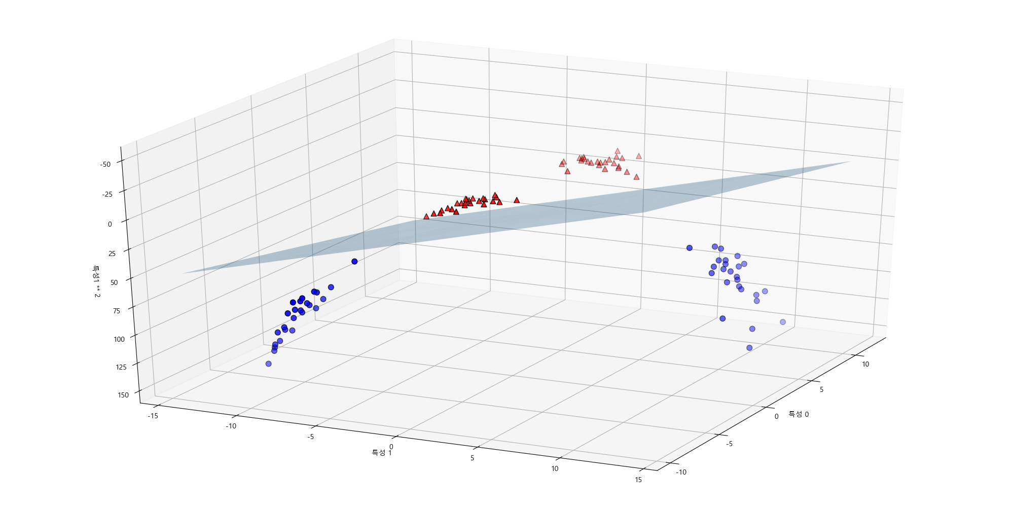
Example:
Imagine predicting whether a company will be profitable (1) or not (0) based on:
- Marketing Budget ($ x_1 $)
- R&D Investment ($ x_2 $)
- Number of Employees ($ x_3 $)
The decision boundary would be a plane in 3D space, separating profitable and non-profitable companies.
In general, for n features, the decision boundary is a hyperplane in an n-dimensional space.
4. Non-Linear Decision Boundaries in Depth
So far, we have seen that logistic regression creates linear decision boundaries. However, many real-world problems have non-linear relationships. In such cases, a straight line (or plane) is not sufficient to separate classes.
To capture complex decision boundaries, we introduce polynomial features or feature transformations.
Example 1: Circular Decision Boundary
If the data requires a circular boundary, we can use quadratic terms:
$$ \theta_0 + \theta_1 x_1^2 + \theta_2 x_2^2 = 0 $$
This represents a circle in 2D space.
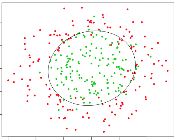
For example:
-
If $ x_1 $ and $ x_2 $ are the coordinates of points, a decision boundary like:
$$ x_1^2 + x_2^2 = 4 $$
would classify points inside a radius-2 circle as Class 1 and outside as Class 0.
Example 2: Elliptical Decision Boundary
A more general quadratic equation:
$$ \theta_0 + \theta_1 x_1^2 + \theta_2 x_2^2 + \theta_3 x_1 x_2 = 0 $$
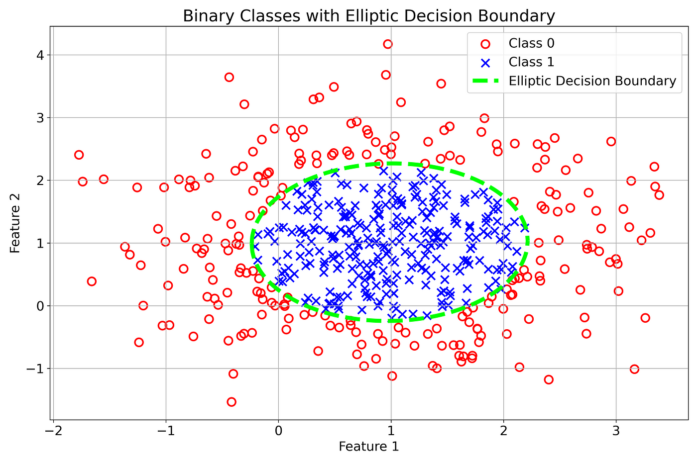
This allows for elliptical decision boundaries.
Example 3: Complex Non-Linear Boundaries
For even more complex boundaries, we can include higher-order polynomial features, such as:
$$ \theta_0 + \theta_1 x_1 + \theta_2 x_2 + \theta_3 x_1^2 + \theta_4 x_2^2 + \theta_5 x_1 x_2 + \theta_6 x_1^3 + \theta_7 x_2^3 = 0 $$
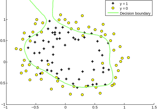
This enables twists and curves in the decision boundary, allowing logistic regression to model highly non-linear patterns.
Feature Engineering for Non-Linear Boundaries
- Instead of adding polynomial terms manually, we can transform features using basis functions (e.g., Gaussian kernels or radial basis functions).
- Feature maps can convert non-linearly separable data into a higher-dimensional space where a linear decision boundary works.
Limitations of Logistic Regression for Non-Linear Boundaries
- Feature engineering is required: Unlike neural networks or decision trees, logistic regression cannot learn complex boundaries automatically.
- Higher-degree polynomials can lead to overfitting: Too many non-linear terms make the model sensitive to noise.
Key Takeaways
- In 3D, the decision boundary is a plane, and in higher dimensions, it becomes a hyperplane.
- Non-linear decision boundaries can be created using quadratic, cubic, or transformed features.
- Feature engineering is crucial to make logistic regression work well for non-linearly separable problems.
- Too many high-order polynomial terms can cause overfitting, so regularization is needed.
3. Cost Function for Logistic Regression
1. Why Do We Need a Cost Function?
In linear regression, we use the Mean Squared Error (MSE) as the cost function:
$$ J(\theta) = \frac{1}{m} \sum_{i=1}^{m} (h_θ(x_i) - y_i)^2 $$
However, this cost function does not work well for logistic regression because:
- The hypothesis function in logistic regression is non-linear due to the sigmoid function.
- Using squared errors results in a non-convex function with multiple local minima, making optimization difficult.
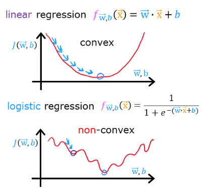
We need a different cost function that:
✅ Works well with the sigmoid function.
✅ Is convex, so gradient descent can efficiently minimize it.
2. Simplified Cost Function for Logistic Regression
Instead of using squared errors, we use a log loss function:
$$ J(\theta) = -\frac{1}{m} \sum_{i=1}^{m} \left[ y_i \log(h_θ(x_i)) + (1 - y_i) \log(1 - h_θ(x_i)) \right] $$
Where:
- $ y_i $ is the true label (0 or 1).
- $ h_θ(x_i) $ is the predicted probability from the sigmoid function.
This function ensures:
- If $ y = 1 $ → The first term dominates: $ -\log(h_θ(x)) $, which is close to 0 if $ h_\theta(x) \approx 1 $ (correct prediction).
- If $ y = 0 $ → The second term dominates: $ -\log(1 - h_θ(x)) $, which is close to 0 if $ h_\theta(x) \approx 0 $.
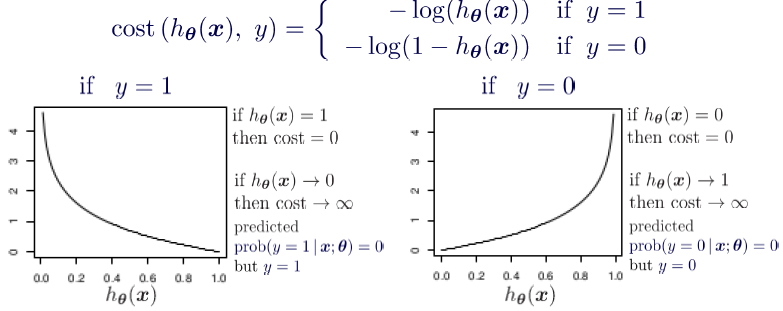
✅ Interpretation: The function penalizes incorrect predictions heavily while rewarding correct predictions.
3. Intuition Behind the Cost Function
Let’s break it down:
-
When $ y = 1 $, the cost function simplifies to:
$$ -\log(h_θ(x)) $$
This means:
- If $ h_θ(x) \approx 1 $ (correct prediction), $ -\log(1) = 0 $ → No penalty.
- If $ h_θ(x) \approx 0 $ (wrong prediction), $ -\log(0) \to \infty $ → High penalty!
-
When $ y = 0 $, the cost function simplifies to:
$$ -\log(1 - h_θ(x)) $$
This means:
- If $ h_θ(x) \approx 0 $ (correct prediction), $ -\log(1) = 0 $ → No penalty.
- If $ h_θ(x) \approx 1 $ (wrong prediction), $ -\log(0) \to \infty $ → High penalty!
✅ Key Takeaway:
The function assigns very high penalties for incorrect predictions, encouraging the model to learn correct classifications.
4. Gradient Descent for Logistic Regression
1. Why Do We Need Gradient Descent?
In logistic regression, our goal is to find the best parameters $ \theta $ that minimize the cost function:
$$ J(\theta) = -\frac{1}{m} \sum_{i=1}^{m} \left[ y_i \log(h_{\theta}(x_i)) + (1 - y_i) \log(1 - h_{\theta}(x_i)) \right] $$
Since there is no closed-form solution like in linear regression, we use gradient descent to iteratively update $ \theta $ until we reach the minimum cost.
2. Gradient Descent Algorithm
Gradient descent updates the parameters using the rule:
$$ \theta_j := \theta_j - \alpha \frac{\partial J(\theta)}{\partial \theta_j} $$
Where:
- $ \alpha $ is the learning rate (step size).
- $ \frac{\partial J(\theta)}{\partial \theta_j} $ is the gradient (direction of steepest increase).
For logistic regression, the derivative of the cost function is:
$$ \frac{\partial J(\theta)}{\partial \theta_j} = \frac{1}{m} \sum_{i=1}^{m} (h_{\theta}(x_i) - y_i) x_{ij} $$
Thus, the update rule becomes:
$$ \theta_j := \theta_j - \alpha \frac{1}{m} \sum_{i=1}^{m} (h_{\theta}(x_i) - y_i) x_{ij} $$
✅ Key Insight:
- We compute the error: $ h_θ(x_i) - y_i $.
- Multiply it by the feature $ x_{ij} $.
- Average over all training examples.
- Scale by $ \alpha $ and update $ \theta_j $.
Overfitting and Regularization
- 1. The Problem of Overfitting
- 2. Addressing Overfitting
- 3. Regularized Cost Function
- 4. Regularized Linear Regression
- 5. Regularized Logistic Regression
1. The Problem of Overfitting
What is Overfitting?
Overfitting occurs when a machine learning model learns the training data too well, capturing noise and random fluctuations rather than the underlying pattern. As a result, the model performs well on training data but generalizes poorly to unseen data.
Symptoms of Overfitting
- High training accuracy but low test accuracy (poor generalization).
- Complex decision boundaries that fit training data too closely.
- Large model parameters (high magnitude weights), leading to excessive sensitivity to small changes in input data.
Example of Overfitting in Regression
Consider a polynomial regression model. If we fit a high-degree polynomial to data, the model may pass through all training points perfectly but fail to predict new data correctly.
Overfitting vs. Underfitting
| Model Complexity | Training Error | Test Error | Generalization |
|---|---|---|---|
| Underfitting (High Bias) | High | High | Poor |
| Good Fit | Low | Low | Good |
| Overfitting (High Variance) | Very Low | High | Poor |
Visualization of Overfitting
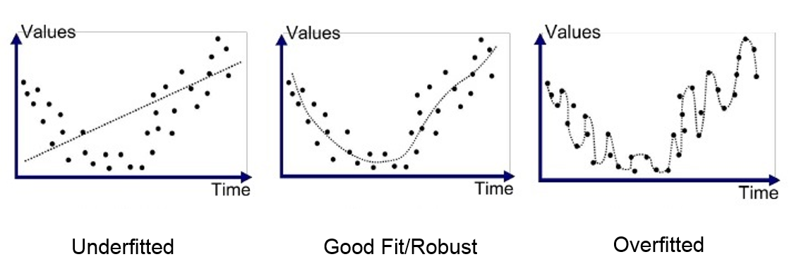
- Left (Underfitting): The model is too simple and cannot capture the trend.
- Middle (Good Fit): The model captures the pattern without overcomplicating.
- Right (Overfitting): The model follows the training data too closely, failing on new inputs.
2. Addressing Overfitting
Overfitting occurs when a model learns noise instead of the underlying pattern in the data. To address overfitting, we can apply several strategies to improve the model’s ability to generalize to unseen data.
1. Collecting More Data
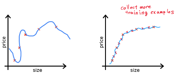
- More training data helps the model capture real patterns rather than memorizing noise.
- Especially effective for deep learning models, where small datasets tend to overfit quickly.
- Not always feasible, but can be supplemented with data augmentation techniques.
2. Feature Selection & Engineering
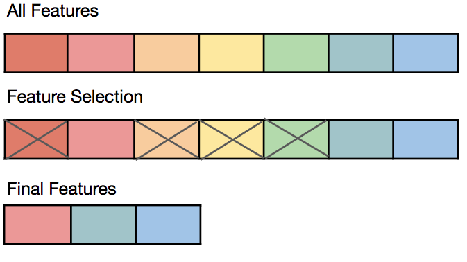
- Removing irrelevant or redundant features reduces model complexity.
- Techniques like Principal Component Analysis (PCA) help reduce dimensionality.
- Engineering new features (e.g., creating polynomial features or interaction terms) can improve generalization.
3. Cross-Validation
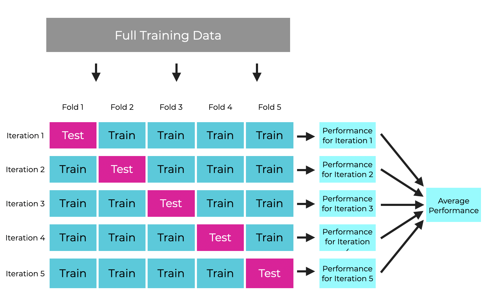
- k-fold cross-validation ensures that the model performs well on different data splits.
- Helps detect overfitting early by testing the model on multiple subsets of data.
- Leave-one-out cross-validation (LOOCV) is another approach, especially useful for small datasets.
4. Regularization as a Solution
- Regularization techniques add constraints to the model to prevent excessive complexity.
- L1 (Lasso) and L2 (Ridge) Regularization introduce penalties for large coefficients.
- We will explore regularized cost functions in the next section.
By applying these techniques, we control model complexity and improve generalization performance. In the next section, we will dive deeper into regularization and its role in the cost function.
3. Regularized Cost Function
Overfitting often occurs when a model learns excessive complexity, leading to poor generalization. One way to control this is by modifying the cost function to penalize overly complex models.
1. Why Modify the Cost Function?
The standard cost function in regression or classification only minimizes the error on training data, which can result in large coefficients (weights) that overfit the data.
By adding a regularization term, we discourage large weights, making the model simpler and reducing overfitting.
2. Adding Regularization Term
Regularization adds a penalty term to the cost function that shrinks the model parameters. The two most common types of regularization are:
L2 Regularization (Ridge Regression)
In L2 regularization, we add the sum of squared weights to the cost function:
$$ J(\theta) = \frac{1}{m} \sum_{i=1}^{m} \left[ h_\theta(x^{(i)}) - y^{(i)} \right]^2 + \lambda \sum_{j=1}^{n} \theta_j^2 $$
- $\lambda$ (regularization parameter) controls how much regularization is applied.
- Higher $\lambda$ values force the model to reduce the magnitude of parameters, preventing overfitting.
- L2 regularization keeps all features but reduces their impact.
L1 Regularization (Lasso Regression)
In L1 regularization, we add the absolute values of weights:
$$ J(\theta) = \frac{1}{m} \sum_{i=1}^{m} \left[ h_\theta(x^{(i)}) - y^{(i)} \right]^2 + \lambda \sum_{j=1}^{n} |\theta_j| $$
- L1 regularization pushes some coefficients to zero, effectively performing feature selection.
- It results in sparser models, which are useful when many features are irrelevant.
3. Effect of Regularization on Model Complexity
Regularization controls model complexity by restricting parameter values:
- No Regularization ($\lambda = 0$) → The model fits the training data too closely (overfitting).
- Small $\lambda$ → The model is still flexible but generalizes better.
- Large $\lambda$ → The model becomes too simple (underfitting), losing important patterns.
Visualization of Regularization Effects
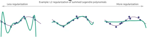
- Left (No Regularization): The model overfits training data.
- Middle (Moderate Regularization): The model generalizes well.
- Right (Strong Regularization): The model underfits the data.
4. Regularized Linear Regression
Linear regression without regularization can suffer from overfitting, especially when the model has too many features or when training data is limited. Regularization helps by constraining the model’s parameters, preventing extreme values that lead to high variance.
1. Linear Regression Cost Function (Without Regularization)
The standard cost function for linear regression is:
$$ J(\theta) = \frac{1}{2m} \sum_{i=1}^{m} \left( h_\theta(x^{(i)}) - y^{(i)} \right)^2 $$
where:
- $ h_\theta(x) = \theta^T x $ is the hypothesis (predicted value),
- $ m $ is the number of training examples.
This function minimizes the sum of squared errors but does not impose any restrictions on the parameter values, which can lead to overfitting.
2. Regularized Cost Function for Linear Regression
To prevent overfitting, we add an L2 regularization term (also known as Ridge Regression) to penalize large parameter values:
$$ J(\theta) = \frac{1}{2m} \sum_{i=1}^{m} \left( h_\theta(x^{(i)}) - y^{(i)} \right)^2 + \frac{\lambda}{2m} \sum_{j=1}^{n} \theta_j^2 $$
where:
- $ \lambda $ is the regularization parameter that controls the penalty,
- The term $ \sum \theta_j^2 $ penalizes large values of $ \theta $,
- $ \theta_0 $ (bias term) is not regularized.
3. Effect of Regularization in Gradient Descent
Regularization modifies the gradient descent update rule:
$$ \theta_j := \theta_j - \alpha \left[ \frac{1}{m} \sum_{i=1}^{m} \left( h_\theta(x^{(i)}) - y^{(i)} \right) x_j + \frac{\lambda}{m} \theta_j \right] $$
- The additional term $ \frac{\lambda}{m} \theta_j $ shrinks the parameter values over time.
- When $ \lambda $ is too large, the model underfits (too simple).
- When $ \lambda $ is too small, the model overfits (too complex).
Effect of Regularization on Parameters
- If $ \lambda = 0 $: Regularization is off → Overfitting risk.
- If $ \lambda $ is too high: Model is too simple → Underfitting.
- If $ \lambda $ is optimal: Good generalization → Balanced model.
4. Normal Equation with Regularization
For linear regression, we can solve for $ \theta $ using the Normal Equation, which avoids gradient descent:
$$ \theta = (X^T X + \lambda I)^{-1} X^T y $$
where:
- $ I $ is the identity matrix (except $ \theta_0 $ is not regularized).
- Adding $ \lambda I $ ensures $ X^T X $ is invertible, reducing multicollinearity issues.
5. Summary
✅ Regularization reduces overfitting by penalizing large weights.
✅ L2 regularization (Ridge Regression) modifies cost function by adding $ \sum \theta_j^2 $.
✅ Gradient Descent and Normal Equation both adjust to include regularization.
✅ Choosing $ \lambda $ is critical: too high → underfitting, too low → overfitting.
5. Regularized Logistic Regression
Logistic regression is commonly used for classification tasks, but like linear regression, it can overfit when there are too many features or limited data. Regularization helps control overfitting by penalizing large parameter values.
1. Logistic Regression Cost Function (Without Regularization)
The standard cost function for logistic regression is:
$$ J(\theta) = -\frac{1}{m} \sum_{i=1}^{m} \left[ y^{(i)} \log h_\theta(x^{(i)}) + (1 - y^{(i)}) \log (1 - h_\theta(x^{(i)})) \right] $$
where:
- $ h_\theta(x) = \frac{1}{1 + e^{-\theta^T x}} $ is the sigmoid function,
- $ y $ is the actual class label ($ 0 $ or $ 1 $),
- $ m $ is the number of training examples.
This cost function does not include regularization, meaning the model may assign large weights to some features, leading to overfitting.
2. Regularized Cost Function for Logistic Regression
To reduce overfitting, we add an L2 regularization term, similar to regularized linear regression:
$$ J(\theta) = -\frac{1}{m} \sum_{i=1}^{m} \left[ y^{(i)} \log h_\theta(x^{(i)}) + (1 - y^{(i)}) \log (1 - h_\theta(x^{(i)})) \right] + \frac{\lambda}{2m} \sum_{j=1}^{n} \theta_j^2 $$
where:
- $ \lambda $ is the regularization parameter (controls penalty),
- The term $ \sum \theta_j^2 $ discourages large parameter values,
- $ \theta_0 $ (bias term) is NOT regularized.
✅ Effect of Regularization
- Small $ \lambda $ → Model may overfit (complex decision boundary).
- Large $ \lambda $ → Model may underfit (too simple, missing important features).
- Optimal $ \lambda $ → Model generalizes well.
3. Effect of Regularization in Gradient Descent
Regularization modifies the gradient descent update rule:
$$ \theta_j := \theta_j - \alpha \left[ \frac{1}{m} \sum_{i=1}^{m} \left( h_\theta(x^{(i)}) - y^{(i)} \right) x_j + \frac{\lambda}{m} \theta_j \right] $$
- The regularization term $ \frac{\lambda}{m} \theta_j $ shrinks the weight values over time.
- Helps avoid models that memorize training data instead of learning patterns.
4. Decision Boundary and Regularization
Regularization also affects decision boundaries:
- Without regularization ($ \lambda = 0 $): Complex boundaries that fit noise.
- With moderate $ \lambda $: Simpler boundaries that generalize better.
- With very high $ \lambda $: Too simplistic boundaries that underfit.
5. Summary
✅ Regularization in logistic regression prevents overfitting by controlling parameter sizes.
✅ L2 regularization (Ridge Regression) adds $ \sum \theta_j^2 $ to cost function.
✅ Gradient Descent is adjusted to shrink large weights.
✅ Choosing $ \lambda $ is critical for a well-generalized model.
Scikit-learn: Practical Applications
- 1. Introduction to Scikit-Learn
- 2. Linear Regression with Scikit-Learn
- 3. Multiple Linear Regression with Scikit-Learn
- 4. Polynomial Regression with Scikit-Learn
- 5. Binary Classification with Logistic Regression
- 6. Multi-Class Classification with Logistic Regression
1. Introduction to Scikit-Learn
Scikit-Learn is one of the most popular and powerful Python libraries for machine learning. It provides efficient implementations of various machine learning algorithms and tools for data preprocessing, model selection, and evaluation. It is built on top of NumPy, SciPy, and Matplotlib, making it highly compatible with the scientific computing ecosystem in Python.
Why Use Scikit-Learn?
- Easy to Use: Provides a simple and consistent API for machine learning models.
- Comprehensive: Includes a wide range of algorithms, including regression, classification, clustering, and dimensionality reduction.
- Efficient: Implements fast and optimized versions of ML algorithms.
- Integration: Works well with other libraries like Pandas, NumPy, and Matplotlib.
Loading Built-in Datasets in Scikit-Learn
Scikit-Learn provides several built-in datasets that can be used for practice and experimentation. Some common datasets include:
- Iris Dataset (
load_iris): Classification dataset for flower species. - Boston Housing Dataset (
load_boston) (Deprecated): Regression dataset for predicting house prices. - Digits Dataset (
load_digits): Handwritten digit classification. - Wine Dataset (
load_wine): Classification dataset for different types of wine. - Breast Cancer Dataset (
load_breast_cancer): Binary classification dataset for cancer diagnosis.
Example: Loading and Exploring the Iris Dataset
from sklearn.datasets import load_iris
import pandas as pd
# Load the dataset
iris = load_iris()
# Convert to DataFrame
iris_df = pd.DataFrame(iris.data, columns=iris.feature_names)
# Add target labels
iris_df['target'] = iris.target
# Display first few rows
print(iris_df.head())
Splitting Data: Train-Test Split
To evaluate a machine learning model, we need to split the data into a training set and a test set. This ensures that we can measure the model’s performance on unseen data.
Scikit-Learn provides train_test_split for this purpose:
Example: Splitting the Iris Dataset
from sklearn.model_selection import train_test_split
# Features and target variable
X = iris.data
y = iris.target
# Split into 80% training and 20% testing
X_train, X_test, y_train, y_test = train_test_split(X, y, test_size=0.2, random_state=42)
print(f"Training samples: {len(X_train)}, Testing samples: {len(X_test)}")
test_size=0.2means 20% of the data is reserved for testing.random_state=42ensures reproducibility.
By following these steps, we have successfully loaded a dataset and prepared it for machine learning. In the next section, we will explore how to apply Linear Regression using Scikit-Learn.
Train-Test Split and Why It Matters
When training a machine learning model, we must evaluate its performance on unseen data to ensure it generalizes well. This is done by splitting the dataset into training and test sets.
Why Not Use 100% of Data for Training?
If we train the model using all available data, we won’t have any independent data to check how well it performs on new inputs. This leads to overfitting, where the model memorizes the training data instead of learning general patterns.
Why Not Use 90% or More for Testing?
While a large test set gives a better estimate of real-world performance, it reduces the amount of data available for training. A model trained on very little data may suffer from underfitting—it won’t have enough information to learn meaningful patterns.
What’s the Ideal Train-Test Split?
A commonly used ratio is 80% for training, 20% for testing. However, this depends on:
- Dataset Size: If data is limited, we may use a 90/10 split to keep more training data.
- Model Complexity: Simpler models may work with less training data, but deep learning models require more.
- Use Case: In critical applications (e.g., medical diagnosis), a larger test set (e.g., 30%) is preferred for reliable evaluation.
Key Takeaways
✅ 80/20 is a good starting point, but can vary based on dataset size and model needs.
✅ Too small a test set → Unreliable performance evaluation.
✅ Too large a test set → Model may not have enough training data to learn properly.
✅ Always shuffle the data before splitting to avoid biased results.
2. Linear Regression with Scikit-Learn
1. Introduction to Linear Regression
Linear regression is a fundamental supervised learning algorithm used to model the relationship between a dependent variable (target) and one or more independent variables (features). It assumes a linear relationship between input features and the output.
The mathematical form of a simple linear regression model is:
$$ y = \theta_0 + \theta_1 x $$
Where:
- $y$ is the predicted output.
- $x$ is the input feature.
- $\theta_0$ is the intercept (bias).
- $\theta_1$ is the coefficient (weight) of the feature.
Now, let’s implement a simple linear regression model using Scikit-Learn.
2. Importing Required Libraries
First, we import necessary libraries for handling data, building the model, and evaluating its performance.
import numpy as np
import matplotlib.pyplot as plt
import pandas as pd
from sklearn.model_selection import train_test_split
from sklearn.linear_model import LinearRegression
from sklearn.metrics import mean_squared_error, r2_score
3. Creating a Sample Dataset
We will generate a synthetic dataset to train and test our linear regression model.
# Generate random data
np.random.seed(42) # Ensures reproducibility
X = 2 * np.random.rand(100, 1) # 100 samples, single feature
y = 4 + 3 * X + np.random.randn(100, 1) # y = 4 + 3X + Gaussian noise
# Convert to a DataFrame for better visualization
df = pd.DataFrame(np.hstack((X, y)), columns=["Feature X", "Target y"])
df.head()
np.random.rand(100, 1): Generates $100$ random values between $0$ and $2$.y = 4 + 3X + noise: Defines a linear relationship with some added noise.- We use
pd.DataFrameto display the first few samples.
4. Splitting Data into Training and Testing Sets
It is crucial to split the dataset into training and testing sets to evaluate model performance on unseen data.
# Splitting dataset into 80% training and 20% testing
X_train, X_test, y_train, y_test = train_test_split(X, y, test_size=0.2, random_state=42)
print(f"Training set size: {X_train.shape[0]} samples")
print(f"Testing set size: {X_test.shape[0]} samples")
5. Training the Linear Regression Model
Now, we train a linear regression model using Scikit-Learn’s LinearRegression() class.
# Create and train the model
model = LinearRegression()
model.fit(X_train, y_train)
# Print learned parameters
print(f"Intercept (theta_0): {model.intercept_[0]:.2f}")
print(f"Coefficient (theta_1): {model.coef_[0][0]:.2f}")
fit(X_train, y_train): Trains the model by finding the best-fitting line.model.intercept_: The learned bias term.model.coef_: The learned weight for the feature.
6. Making Predictions
After training, we make predictions on the test set.
# Predict on test data
y_pred = model.predict(X_test)
# Compare actual vs predicted values
comparison_df = pd.DataFrame({"Actual": y_test.flatten(), "Predicted": y_pred.flatten()})
comparison_df.head()
model.predict(X_test): Generates predictions.- The DataFrame compares actual vs. predicted values.
7. Evaluating the Model
We use Mean Squared Error (MSE) and R² Score to evaluate model performance.
# Calculate Mean Squared Error (MSE)
mse = mean_squared_error(y_test, y_pred)
# Calculate R-squared score
r2 = r2_score(y_test, y_pred)
print(f"Mean Squared Error: {mse:.2f}")
print(f"R-squared Score: {r2:.2f}")
- MSE: Measures average squared differences between actual and predicted values (lower is better).
- R² Score: Measures how well the model explains the variance in the data (closer to 1 is better).
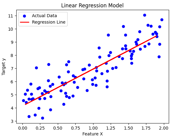
8. Visualizing the Results
Finally, let’s plot the data and the regression line.
plt.scatter(X, y, color="blue", label="Actual Data")
plt.plot(X_test, y_pred, color="red", linewidth=2, label="Regression Line")
plt.xlabel("Feature X")
plt.ylabel("Target y")
plt.title("Linear Regression Model")
plt.legend()
plt.show()
This plot shows:
- Blue points → Actual test data
- Red line → Best-fit regression line
3. Multiple Linear Regression with Scikit-Learn
What is Multiple Linear Regression?
Multiple Linear Regression is an extension of simple linear regression where we predict a dependent variable ($y$) using multiple independent variables ($x_1, x_2, …, x_n$). The general form of the equation is:
$$ y = \theta_0 + \theta_1 x_1 + \theta_2 x_2 + … + \theta_n x_n $$
Where:
- $ y $ = predicted output
- $ x_1, x_2, …, x_n $ = independent variables (features)
- $ \theta_0 $ = intercept
- $ \theta_1, \theta_2, …, \theta_n $ = coefficients (weights)
In this section, we will:
- Generate a synthetic dataset for a multiple linear regression model.
- Train a model using Scikit-Learn.
- Visualize the relationship in a 3D plot.
Step 1: Generate a Synthetic Dataset
First, let’s create a dataset with two independent variables ($x_1$ and $x_2$) and one dependent variable ($y$). We’ll add some noise to make it more realistic.
import numpy as np
import matplotlib.pyplot as plt
from mpl_toolkits.mplot3d import Axes3D
from sklearn.linear_model import LinearRegression
from sklearn.model_selection import train_test_split
# Set seed for reproducibility
np.random.seed(42)
# Generate random data for x1 and x2
x1 = np.random.uniform(0, 10, 100)
x2 = np.random.uniform(0, 10, 100)
# Define the true equation y = 3 + 2*x1 + 1.5*x2 + noise
y = 3 + 2*x1 + 1.5*x2 + np.random.normal(0, 2, 100)
# Reshape x1 and x2 for model training
X = np.column_stack((x1, x2))
Step 2: Train the Model
Now, we split the dataset into training and test sets and train a multiple linear regression model.
# Split data into training and test sets
X_train, X_test, y_train, y_test = train_test_split(X, y, test_size=0.2, random_state=42)
# Create and train the model
model = LinearRegression()
model.fit(X_train, y_train)
# Get model parameters
theta0 = model.intercept_
theta1, theta2 = model.coef_
print(f"Model equation: y = {theta0:.2f} + {theta1:.2f}*x1 + {theta2:.2f}*x2")
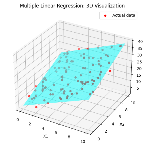
Step 3: Visualize the Regression Plane
Since we have two independent variables ($x_1$ and $x_2$), we can plot the regression plane in 3D space.
# Generate grid for x1 and x2
x1_range = np.linspace(0, 10, 20)
x2_range = np.linspace(0, 10, 20)
x1_grid, x2_grid = np.meshgrid(x1_range, x2_range)
# Compute predicted y values
y_pred_grid = theta0 + theta1 * x1_grid + theta2 * x2_grid
# Create 3D plot
fig = plt.figure(figsize=(10, 6))
ax = fig.add_subplot(111, projection='3d')
# Scatter plot of real data
ax.scatter(x1, x2, y, color='red', label='Actual data')
# Regression plane
ax.plot_surface(x1_grid, x2_grid, y_pred_grid, alpha=0.5, color='cyan')
# Labels
ax.set_xlabel('X1')
ax.set_ylabel('X2')
ax.set_zlabel('Y')
ax.set_title('Multiple Linear Regression: 3D Visualization')
plt.legend()
plt.show()
Key Takeaways
- We generated a dataset with two independent variables and one dependent variable.
- We trained a Multiple Linear Regression model using Scikit-Learn.
- We visualized the regression plane in 3D, showing how $x_1$ and $x_2$ influence $y$.
4. Polynomial Regression with Scikit-Learn
Polynomial Regression is an extension of Linear Regression, where we introduce polynomial terms to capture non-linear relationships in the data.
1. What is Polynomial Regression?
Linear regression models relationships using a straight line:
$$ y = \theta_0 + \theta_1 x $$
However, if the data follows a non-linear pattern, a straight line won’t fit well. Instead, we can introduce polynomial terms:
$$ y = \theta_0 + \theta_1 x + \theta_2 x^2 + \theta_3 x^3 + \dots + \theta_n x^n $$
This allows the model to capture curvature in the data.
2. Generating Non-Linear Data
First, let’s create a synthetic dataset with a non-linear relationship.
import numpy as np
import matplotlib.pyplot as plt
# Generate random x values between -3 and 3
np.random.seed(42)
X = np.linspace(-3, 3, 100).reshape(-1, 1)
# Generate a non-linear function with some noise
y = 0.5 * X**3 - X**2 + 2 + np.random.randn(100, 1) * 2
# Scatter plot of the data
plt.scatter(X, y, color='blue', alpha=0.5, label="True Data")
plt.xlabel("X")
plt.ylabel("y")
plt.title("Generated Non-Linear Data")
plt.legend()
plt.show()
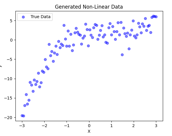
- We create 100 random points between -3 and 3.
- The function we generate follows a cubic equation:
- $y=0.5x^3 −x^2 +2$ with added noise.
- We visualize the data using a scatter plot.
3. Applying Polynomial Features
To transform our linear features into polynomial features, we use PolynomialFeatures from sklearn.preprocessing.
from sklearn.preprocessing import PolynomialFeatures
# Transform X into polynomial features (degree=3)
poly = PolynomialFeatures(degree=3)
X_poly = poly.fit_transform(X)
print(f"Original X shape: {X.shape}")
print(f"Transformed X shape: {X_poly.shape}")
print(f"First 5 rows of X_poly:\n{X_poly[:5]}")
- We use
PolynomialFeatures(degree=3)to add polynomial terms up to $x^3$. - This converts each $𝑥$ value into a feature vector $[1,x,x^2,x^3]$.
- We print the new shape and first few transformed rows.
4. Training a Polynomial Regression Model
Now, we train a Linear Regression model using these polynomial features.
from sklearn.linear_model import LinearRegression
# Train polynomial regression model
model = LinearRegression()
model.fit(X_poly, y)
# Predictions
y_pred = model.predict(X_poly)
5. Visualizing the Results
Let’s plot the polynomial regression model against the actual data.
plt.scatter(X, y, color='blue', alpha=0.5, label="True Data")
plt.plot(X, y_pred, color='red', linewidth=2, label="Polynomial Regression Fit")
plt.xlabel("X")
plt.ylabel("y")
plt.title("Polynomial Regression Model")
plt.legend()
plt.show()
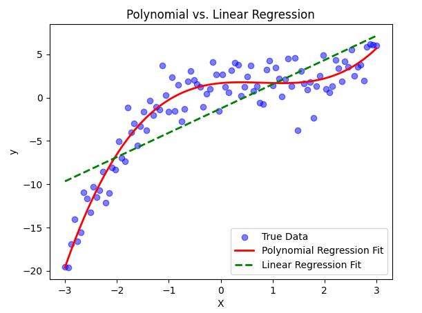
6. Comparing with Linear Regression
Now, let’s compare Polynomial Regression with a simple Linear Regression model.
# Train a simple Linear Regression model
linear_model = LinearRegression()
linear_model.fit(X, y)
y_linear_pred = linear_model.predict(X)
# Plot both models
plt.scatter(X, y, color='blue', alpha=0.5, label="True Data")
plt.plot(X, y_pred, color='red', linewidth=2, label="Polynomial Regression Fit")
plt.plot(X, y_linear_pred, color='green', linestyle="dashed", linewidth=2, label="Linear Regression Fit")
plt.xlabel("X")
plt.ylabel("y")
plt.title("Polynomial vs. Linear Regression")
plt.legend()
plt.show()
5. Binary Classification with Logistic Regression
Logistic Regression is a fundamental algorithm used for binary classification problems. It estimates the probability that a given input belongs to a particular class using the sigmoid function.
1. What is Logistic Regression?
Unlike Linear Regression, which predicts continuous values, Logistic Regression predicts probabilities and then maps them to class labels (0 or 1). The model is defined as:
$$ P(y=1 | X) = \frac{1}{1 + e^{-\theta^T X}} $$
Where:
- $\theta$ represents the model parameters (weights and bias).
- $X$ represents the input features.
- The output is a probability between 0 and 1.
2. Generating a Synthetic Dataset (Spam Detection Example)
We’ll create a synthetic dataset where emails are classified as spam (1) or not spam (0) based on two features:
- Number of suspicious words
- Email length
import numpy as np
import matplotlib.pyplot as plt
from sklearn.model_selection import train_test_split
from sklearn.linear_model import LogisticRegression
from sklearn.metrics import accuracy_score
# Generating synthetic data
np.random.seed(42)
num_samples = 200
# Feature 1: Number of suspicious words (randomly chosen values)
suspicious_words = np.random.randint(0, 20, num_samples)
# Feature 2: Email length (short emails tend to be spammy)
email_length = np.random.randint(20, 300, num_samples)
# Labels: Spam (1) or Not Spam (0)
labels = (suspicious_words + email_length / 50 > 10).astype(int)
# Creating feature matrix
X = np.column_stack((suspicious_words, email_length))
y = labels
# Splitting into training and testing sets
X_train, X_test, y_train, y_test = train_test_split(X, y, test_size=0.2, random_state=42)
3. Training the Logistic Regression Model
Now, we train a Logistic Regression model on our dataset.
# Training the model
model = LogisticRegression()
model.fit(X_train, y_train)
# Making predictions
y_pred = model.predict(X_test)
# Evaluating the model
accuracy = accuracy_score(y_test, y_pred)
print(f"Model Accuracy: {accuracy:.2f}")
4. Visualizing Decision Boundary
The decision boundary helps us see how the model separates spam from non-spam emails. We plot the boundary in 2D.
# Function to plot decision boundary
def plot_decision_boundary(model, X, y):
x_min, x_max = X[:, 0].min() - 1, X[:, 0].max() + 1
y_min, y_max = X[:, 1].min() - 10, X[:, 1].max() + 10
xx, yy = np.meshgrid(np.linspace(x_min, x_max, 100),
np.linspace(y_min, y_max, 100))
Z = model.predict(np.c_[xx.ravel(), yy.ravel()])
Z = Z.reshape(xx.shape)
plt.contourf(xx, yy, Z, alpha=0.3, cmap=plt.cm.coolwarm)
plt.scatter(X[:, 0], X[:, 1], c=y, edgecolors='k', cmap=plt.cm.coolwarm)
plt.xlabel("Suspicious Words Count")
plt.ylabel("Email Length")
plt.title("Logistic Regression Decision Boundary")
plt.show()
# Plotting the decision boundary
plot_decision_boundary(model, X, y)
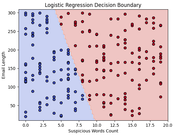
This plot shows how the model separates spam and non-spam emails using our two features.
Key Takeaways
- Logistic Regression is used for binary classification.
- It estimates probabilities using the sigmoid function.
- We generated a synthetic dataset mimicking spam detection.
- We trained and evaluated a Logistic Regression model.
- Decision boundaries help visualize how the model classifies data.
6. Multi-Class Classification with Logistic Regression
In this section, we will implement a Multi-Class Classification model using Logistic Regression. Instead of a binary classification problem, we will classify data points into three distinct categories.
This project predicts a student’s success level based on study hours and past grades using Logistic Regression.
We classify students into three categories:
- Fail (0)
- Pass (1)
- High Pass (2)
Step 1: Import Libraries
We start by importing necessary libraries for:
- Data generation
- Visualization
- Model training
import numpy as np
import matplotlib.pyplot as plt
from sklearn.datasets import make_classification
from sklearn.model_selection import train_test_split
from sklearn.preprocessing import StandardScaler
from sklearn.linear_model import LogisticRegression
from sklearn.metrics import ConfusionMatrixDisplay, classification_report
Step 2: Generate Synthetic Data
We create artificial student data using make_classification.
Each student has:
- Past Grades (0-100)
- Study Hours (non-negative)
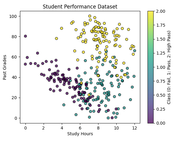
We set random_state = 457897 to ensure reproducibility.
# Generate a classification dataset
X, y = make_classification(n_samples=300,
n_features=2,
n_classes=3,
n_clusters_per_class=1,
n_informative=2,
n_redundant=0,
random_state=457897) # Ensures consistent results
# Normalize Study Hours to be non-negative & scale Past Grades (0-100)
X[:, 0] = X[:, 0] * 12
X[:, 1] = X[:, 1] * 100
# Scatter plot of generated data
plt.figure(figsize=(7, 5))
plt.scatter(X[:, 0], X[:, 1], c=y, cmap='viridis', edgecolors='k', alpha=0.75)
plt.xlabel("Study Hours")
plt.ylabel("Past Grades")
plt.title("Student Performance Dataset")
plt.colorbar(label="Class (0: Fail, 1: Pass, 2: High Pass)")
plt.show()
Step 3: Split the Data
X_train, X_test, y_train, y_test = train_test_split(X, y, test_size=0.2, random_state=457897, stratify=y)
# Standardizing features for better model performance
scaler = StandardScaler()
X_train = scaler.fit_transform(X_train)
X_test = scaler.transform(X_test)
Step 4: Train Logistic Regression Model
from sklearn.multiclass import OneVsRestClassifier
# Define and train the model
model = OneVsRestClassifier(LogisticRegression(solver='lbfgs'))
model.fit(X_train, y_train)
Step 5: Visualizing Decision Boundaries
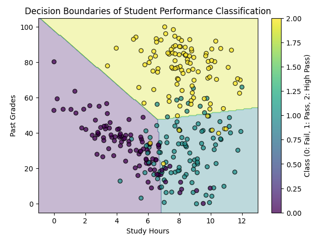
# Define a mesh grid for visualization
x_min, x_max = X[:, 0].min() - 1, X[:, 0].max() + 1
y_min, y_max = X[:, 1].min() - 5, X[:, 1].max() + 5
xx, yy = np.meshgrid(np.linspace(x_min, x_max, 200),
np.linspace(y_min, y_max, 200))
# Predict on the mesh grid
Z = model.predict(scaler.transform(np.c_[xx.ravel(), yy.ravel()]))
Z = Z.reshape(xx.shape)
# Plot decision boundary
plt.figure(figsize=(7, 5))
plt.contourf(xx, yy, Z, alpha=0.3, cmap="viridis")
plt.scatter(X[:, 0], X[:, 1], c=y, cmap="viridis", edgecolors='k', alpha=0.75)
plt.xlabel("Study Hours")
plt.ylabel("Past Grades")
plt.title("Decision Boundaries of Student Performance Classification")
plt.colorbar(label="Class (0: Fail, 1: Pass, 2: High Pass)")
plt.show()
Neural Networks: Intuition and Model
- Understanding Neural Networks
- Biological Inspiration: The Brain and Synapses
- Importance of Layers in Neural Networks
- Face Recognition Example: Layer-by-Layer Processing
- Mathematical Representation of a Neural Network
Understanding Neural Networks
Neural networks are a fundamental concept in deep learning, inspired by the way the human brain processes information. They consist of layers of artificial neurons that transform input data into meaningful outputs. At the core of a neural network is a simple mathematical operation: each neuron receives inputs, applies a weighted sum, adds a bias term, and passes the result through an activation function. This process allows the network to learn patterns and make predictions.
Biological Inspiration: The Brain and Synapses
Artificial neural networks (ANNs) are designed based on the biological structure of the human brain. The brain consists of billions of neurons, interconnected through structures called synapses. Neurons communicate with each other by transmitting electrical and chemical signals, which play a critical role in learning, memory, and decision-making processes.
Structure of a Biological Neuron
Each biological neuron consists of several key components:
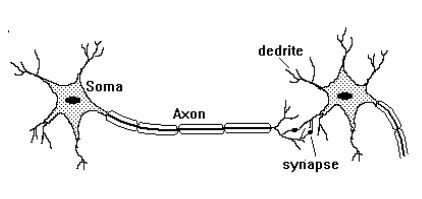
- Dendrites: Receive input signals from other neurons.
- Cell Body (Soma): Processes the received signals and determines whether the neuron should be activated.
- Axon: Transmits the output signal to other neurons.
- Synapses: Junctions between neurons where chemical neurotransmitters facilitate communication.
Artificial Neural Networks vs. Biological Networks
In artificial neural networks:
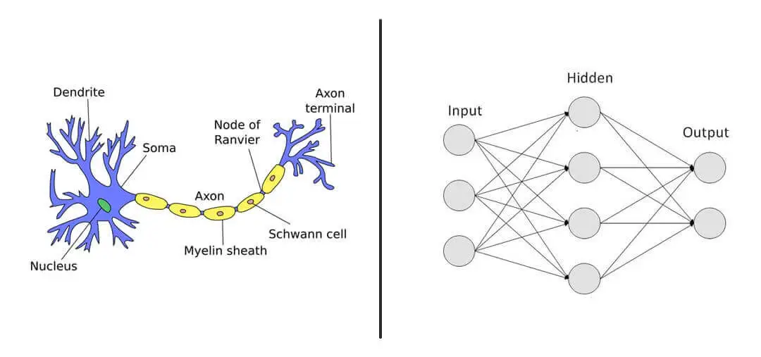
- Neurons function as computational units.
- Weights correspond to synaptic strengths, determining how influential an input is.
- Bias terms help shift the activation threshold.
- Activation functions mimic the way biological neurons fire only when certain thresholds are exceeded.
Importance of Layers in Neural Networks
Neural networks are composed of multiple layers, each responsible for extracting and processing features from input data. The more layers a network has, the deeper it becomes, allowing it to learn complex hierarchical patterns.
Example: Predicting a T-shirt’s Top-Seller Status
Consider an online clothing store that wants to predict whether a new T-shirt will become a top-seller. Several factors influence this outcome, which serve as inputs to our neural network:
- Price ($x_1$)
- Shipping Cost ($x_2$)
- Marketing ($x_3$)
- Material ($x_4$)
These inputs are fed into the first layer of the network, which extracts meaningful features. A possible hidden layer structure could be:
- Hidden Layer 1: Contains a few activations functions like: affordability , awareness, perceived quality.
- Output Layer: Aggregates information from the previous layers to make a final prediction.
The output layer applies a sigmoid activation function:
$$ \sigma(z) = \frac{1}{1 + e^{-z}} $$
where $z$ is a weighted sum of the previous layer’s outputs. If $\sigma(z) > 0.5$, we classify the T-shirt as a top-seller; otherwise, it is not.
Face Recognition Example: Layer-by-Layer Processing
Face recognition is a real-world example where neural networks excel. Let’s consider a deep neural network designed for face recognition, breaking down the processing step by step:
- Input Layer: An image of a face is converted into pixel values (e.g., a 100x100 grayscale image would be represented as a vector of 10,000 pixel values).
- First Hidden Layer: Detects basic edges and corners in the image by applying simple filters.
- Second Hidden Layer: Identifies facial features like eyes, noses, and mouths by combining edge and corner information.
- Third Hidden Layer: Recognizes entire facial structures and relationships between features.
- Output Layer: Determines whether the face matches a known identity by producing a probability score.
Mathematical Representation of a Neural Network
To efficiently compute activations in a neural network, we use matrix notation. The general formula for forward propagation is:
$$ Z^{[l]} = W^{[l]} A^{[l-1]} + b^{[l]} $$
where:
- $ A^{[l-1]} $ is the activation from the previous layer,
- $ W^{[l]} $ is the weight matrix of the current layer,
- $ b^{[l]} $ is the bias vector,
- $ Z^{[l]} $ is the linear combination of inputs before applying the activation function.
The activation function is applied as:
$$ A^{[l]} = g(Z^{[l]}) $$
where $ g $ is typically a sigmoid, ReLU, or softmax function.
Example Calculation
Suppose we have a single-layer neural network with three inputs and one neuron. We define the inputs as:
$$ x_1 = 0.5, \quad x_2 = 0.8, \quad x_3 = 0.2 $$
The corresponding weight matrix and bias term are given by:
$$ W = \left[ \begin{array}{ccc} 0.9 & -0.5 & 0.3 \end{array} \right], \quad b = 0.1 $$
The weighted sum (Z) is calculated as:
$$ Z = W \cdot X + b = (0.5 \times 0.9) + (0.8 \times -0.5) + (0.2 \times 0.3) + 0.1 $$
$$ Z = 0.45 - 0.4 + 0.06 + 0.1 = 0.21 $$
Applying the sigmoid activation function:
$$ \sigma(Z) = \frac{1}{1 + e^{-Z}} = \frac{1}{1 + e^{-0.21}} \approx 0.552 $$
Since the output is above 0.5, we classify this case as positive.
Two Hidden Layer Neural Network Calculation
Now, let’s consider a neural network with two hidden layers.
Network Structure
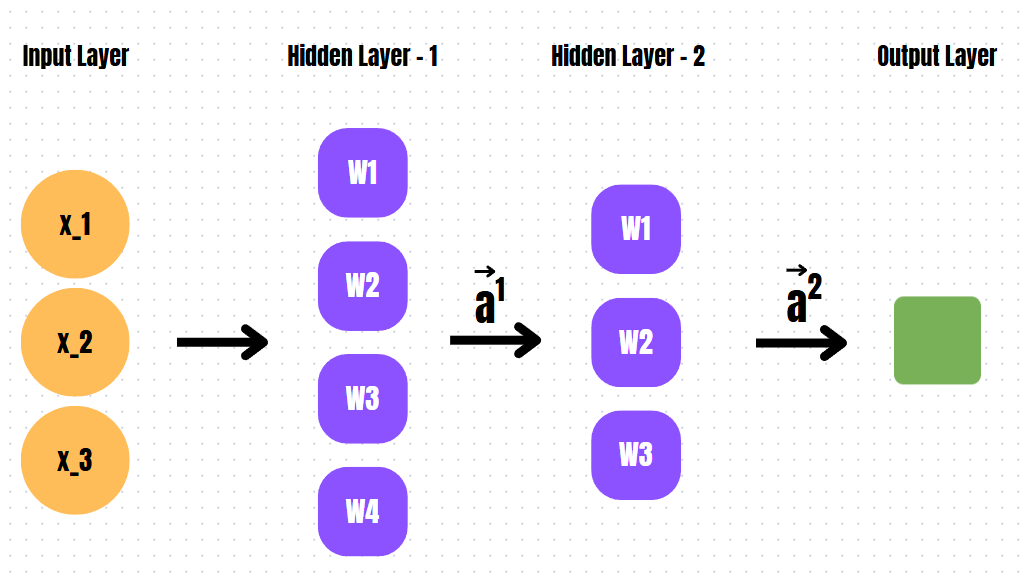
- Input Layer: 3 input values $X = [x_1, x_2, x_3]$
- First Hidden Layer: 4 neurons
- Second Hidden Layer: 3 neurons
- Output Layer: 1 neuron
First Hidden Layer Calculation
Given input vector:
$$ X = \left[ \begin{array}{c} 0.5 \ 0.8 \ 0.2 \end{array} \right] $$
Weight matrix for the first hidden layer:
$$ W^{(1)} = \left[ \begin{array}{ccc} 0.2 & -0.3 & 0.5 \ -0.7 & 0.1 & 0.4 \ 0.3 & 0.8 & -0.6 \ 0.5 & -0.2 & 0.7 \end{array} \right] $$
Bias vector:
$$ b^{(1)} = \left[ \begin{array}{c} 0.1 \ -0.2 \ 0.3 \ 0.4 \end{array} \right] $$
Computing the weighted sum:
$$ Z^{(1)} = W^{(1)}X + b^{(1)} $$
Applying the sigmoid activation function:
$$ A^{(1)} = \sigma(Z^{(1)}) $$
Second Hidden Layer Calculation
Weight matrix:
$$ W^{(2)} = \left[ \begin{array}{cccc} 0.6 & -0.1 & 0.3 & 0.7 \ 0.2 & 0.9 & -0.5 & 0.4 \ -0.3 & 0.5 & 0.7 & -0.6 \end{array} \right] $$
Bias vector:
$$ b^{(2)} = \left[ \begin{array}{c} -0.1 \ 0.3 \ 0.2 \end{array} \right] $$
Computing the weighted sum:
$$ Z^{(2)} = W^{(2)} A^{(1)} + b^{(2)} $$
Applying the sigmoid activation function:
$$ A^{(2)} = \sigma(Z^{(2)}) $$
Output Layer Calculation
Weight matrix:
$$ W^{(3)} = \left[ \begin{array}{ccc} 0.5 & -0.7 & 0.6 \end{array} \right] $$
Bias:
$$ b^{(3)} = -0.2 $$
Computing the final weighted sum:
$$ Z^{(3)} = W^{(3)} A^{(2)} + b^{(3)} $$
Applying the sigmoid activation function:
$$ A^{(3)} = \sigma(Z^{(3)}) $$
If $ A^{(3)} > 0.5 $, the output is classified as positive.
Conclusion
- The first hidden layer extracts basic features.
- The second hidden layer learns more abstract representations.
- The output layer makes the final classification decision.
This demonstrates how a multi-layer neural network processes information in a hierarchical manner.
Handwritten Digit Recognition Using Two Layers
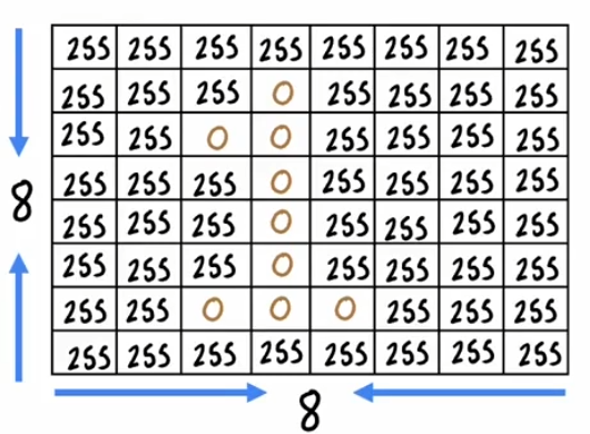
A classic application of neural networks is handwritten digit recognition. Let’s consider recognizing the digit ‘1’ from an 8x8 pixel grid using a simple neural network with two layers.
First Layer: Feature Extraction
- The 8x8 image is flattened into a 64-dimensional input vector.
- This vector is processed by neurons in the first hidden layer.
- The neurons identify edges, curves, and simple shapes using learned weights.
- Mathematically, the output of the first layer can be represented as:
$$ Z^{(1)} = W^{(1)}X + b^{(1)} $$ $$ A^{(1)} = \sigma(Z^{(1)}) $$
Second Layer: Pattern Recognition
- The first layer’s output is passed to a second hidden layer.
- This layer detects digit-specific features, such as the vertical stroke characteristic of ‘1’.
- The transformation at this stage follows:
$$ Z^{(2)} = W^{(2)}A^{(1)} + b^{(2)} $$ $$ A^{(2)} = \sigma(Z^{(2)}) $$
Output Layer: Classification
- The final layer has 10 neurons, each representing a digit from 0 to 9.
- The neuron with the highest activation determines the predicted digit:
$$ Z^{(3)} = W^{(3)}A^{(2)} + b^{(3)} $$ $$ \text{Prediction} = \arg\max(A^{(3)}) $$
This structured approach demonstrates how neural networks model real-world problems, from binary classification to deep learning applications like face and handwriting recognition.
Implementation of Forward Propagation
- Coffee Roasting Example (Classification Task)
- Neural Network Architecture
- TensorFlow Implementation
- Forward Propagation Step-by-Step (NumPy Implementation)
- Artificial General Intelligence (AGI)
Coffee Roasting Example (Classification Task)
Imagine we want to classify coffee as either “Good” or “Bad” based on two factors:
- Temperature (°C)
- Roasting Time (minutes)
For simplicity, we define:
- Good coffee: If the temperature is between 190°C and 210°C and the roasting time is between 10 and 15 minutes.
- Bad coffee: Any other condition.
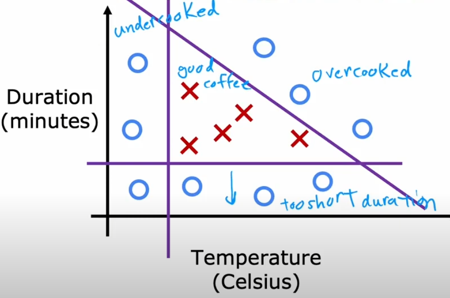
We collect the following data:
| Temperature (°C) | Roasting Time (min) | Quality (1 = Good, 0 = Bad) |
|---|---|---|
| 200 | 12 | 1 |
| 180 | 10 | 0 |
| 210 | 15 | 1 |
| 220 | 20 | 0 |
| 195 | 13 | 1 |
We will implement a simple neural network using TensorFlow to classify new coffee samples.
Neural Network Architecture
We construct a neural network using the following structure:
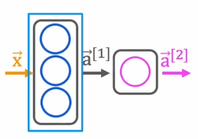
- Input Layer: Two neurons (temperature, time)
- Hidden Layer: Three neurons, activated with the sigmoid function
- Output Layer: One neuron, activated with the sigmoid function (binary classification)
TensorFlow Implementation
Step 1: Importing Libraries
import tensorflow as tf
import numpy as np
tensorflowis the core deep learning library that allows us to define and train neural networks.numpyis used for handling arrays and numerical operations efficiently.
Step 2: Defining Inputs and Outputs
X = np.array([[200, 12], [180, 10], [210, 15], [220, 20], [195, 13]], dtype=np.float32)
y = np.array([[1], [0], [1], [0], [1]], dtype=np.float32)
Xrepresents the input features (temperature and roasting time) as a NumPy array.yrepresents the expected output (1 for good coffee, 0 for bad coffee).dtype=np.float32ensures numerical stability and compatibility with TensorFlow.
Step 3: Building the Model
model = tf.keras.Sequential([
tf.keras.layers.Dense(3, activation='sigmoid', input_shape=(2,)),
tf.keras.layers.Dense(1, activation='sigmoid')
])
Sequential()creates a linear stack of layers.Dense(3, activation='sigmoid', input_shape=(2,))defines the hidden layer:- 3 neurons
- Sigmoid activation function
- Input shape of (2,) since we have two input features.
Dense(1, activation='sigmoid')defines the output layer with 1 neuron and sigmoid activation.
Step 4: Training the Model
model.compile(optimizer='adam', loss='binary_crossentropy', metrics=['accuracy'])
model.fit(X, y, epochs=500, verbose=0)
compile()configures the model for training:adamoptimizer adapts the learning rate automatically.binary_crossentropyis used for binary classification problems.accuracymetric tracks how well the model classifies coffee samples.
fit(X, y, epochs=500, verbose=0)trains the model for 500 epochs (iterations over data).
Step 5: Making Predictions
new_coffee = np.array([[205, 14]], dtype=np.float32)
prediction = model.predict(new_coffee)
print("Prediction (Probability of Good Coffee):", prediction)
new_coffeecontains a new sample (205°C, 14 min) to classify.model.predict(new_coffee)computes the probability of the coffee being good.- The output is a probability (closer to 1 means good, closer to 0 means bad).
Forward Propagation Step-by-Step (NumPy Implementation)
We now implement forward propagation manually using NumPy to understand how TensorFlow executes it under the hood.
Initializing Weights and Biases
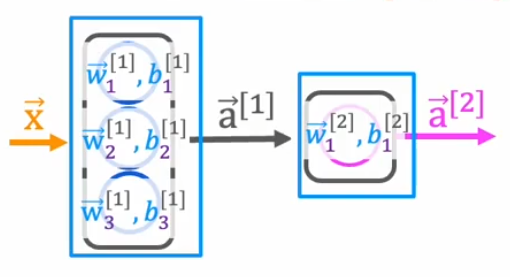
np.random.seed(42) # For reproducibility
W1 = np.random.randn(2, 4) # Weights for hidden layer (2 inputs -> 4 neurons)
b1 = np.random.randn(4) # Bias for hidden layer
W2 = np.random.randn(4, 1) # Weights for output layer (4 neurons -> 1 output)
b2 = np.random.randn(1) # Bias for output layer
np.random.randn()initializes weights and biases randomly from a normal distribution.W1andb1define the hidden layer parameters.W2andb2define the output layer parameters.
Forward Propagation Calculation
def sigmoid(z):
return 1 / (1 + np.exp(-z))
- This function applies the sigmoid activation function, which outputs values between 0 and 1.
def forward_propagation(X):
Z1 = np.dot(X, W1) + b1 # Linear transformation (Hidden Layer)
A1 = sigmoid(Z1) # Activation function (Hidden Layer)
Z2 = np.dot(A1, W2) + b2 # Linear transformation (Output Layer)
A2 = sigmoid(Z2) # Activation function (Output Layer)
return A2
np.dot(X, W1) + b1computes the weighted sum of inputs for the hidden layer.sigmoid(Z1)applies the activation function to introduce non-linearity.np.dot(A1, W2) + b2computes the weighted sum of outputs from the hidden layer.sigmoid(Z2)produces the final prediction.
# Testing with an example input
output = forward_propagation(np.array([[185, 10]]))
print(output)
This manually replicates TensorFlow’s forward propagation but using pure NumPy.
Artificial General Intelligence (AGI)
AGI refers to AI that can perform any intellectual task a human can. Unlike current AI systems, AGI would adapt, learn, and generalize across different tasks without needing task-specific training.
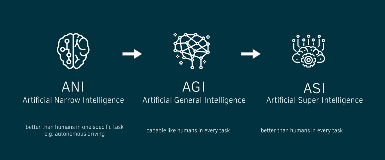
Everyday Example: AGI vs. Narrow AI
- Narrow AI (Current AI): A chess-playing AI can defeat world champions but cannot drive a car.
- AGI: If a chess-playing AI was truly intelligent, it would learn how to drive just like a human without explicit programming.
Key Challenges in AGI
- Transfer Learning: Current AI requires large amounts of data. Humans learn with few examples.
- Common Sense Reasoning: AI struggles with simple logic like “If I drop a glass, it will break.”
- Self-Learning: AGI must improve without needing human intervention.
Is AGI Possible?
- Some scientists believe AGI is decades away, while others argue it may never happen.
- Brain-inspired architectures (like Neural Networks) might be a stepping stone toward AGI.
Neural Network Training and Activation Functions
Understanding Loss Functions
Binary Crossentropy (BCE)
Binary crossentropy is commonly used for binary classification problems. It measures the difference between the predicted probability $ \hat{y} $ and the true label $ y $ as follows:
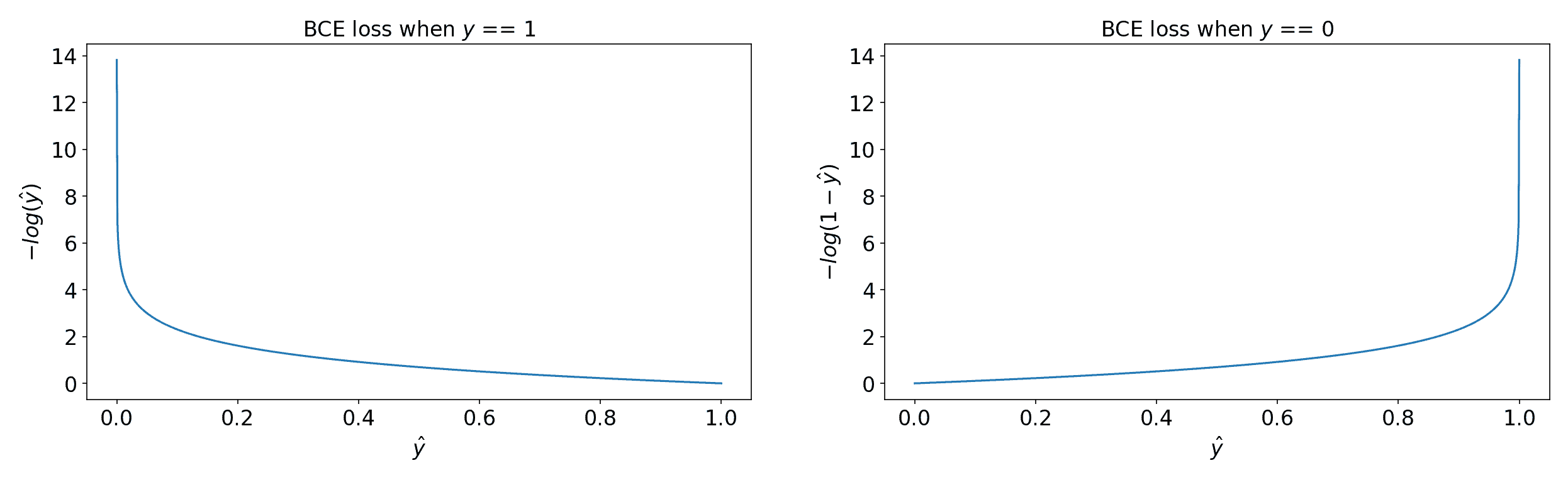
$$ L = - \frac{1}{N} \sum\limits_{i=1}^{N} \left[ y_i \log(\hat{y}_i) + (1 - y_i) \log(1 - \hat{y}_i) \right] $$
TensorFlow Implementation
import tensorflow as tf
loss_fn = tf.keras.losses.BinaryCrossentropy()
y_true = [1, 0, 1, 1]
y_pred = [0.9, 0.1, 0.8, 0.6]
loss = loss_fn(y_true, y_pred)
print("Binary Crossentropy Loss:", loss.numpy())
Mean Squared Error (MSE)
For regression problems, MSE calculates the average squared differences between actual and predicted values:
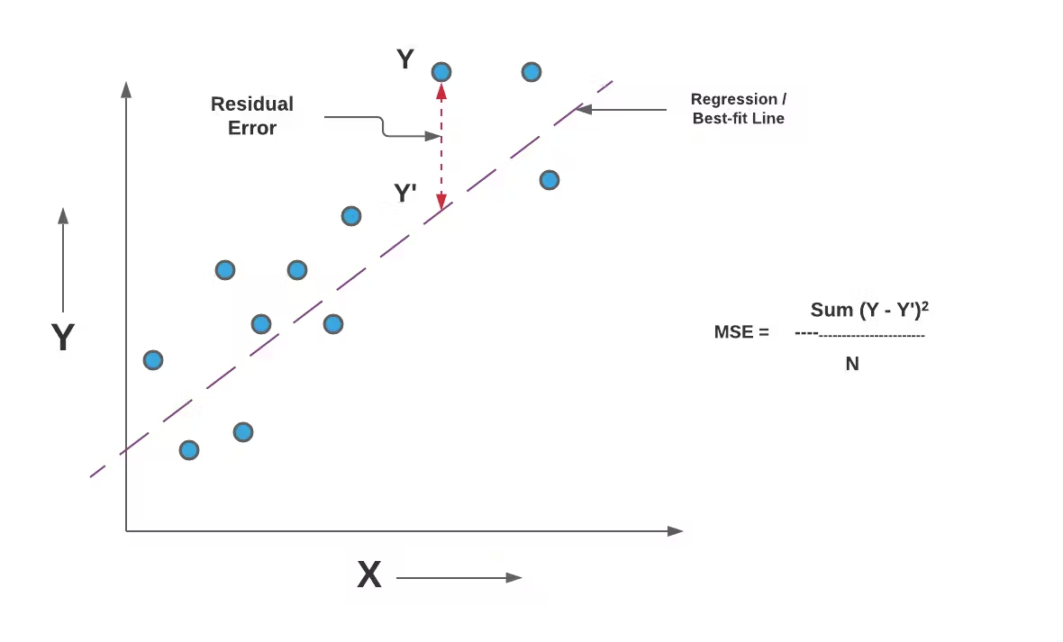
$$ L = \frac{1}{N} \sum\limits_{i=1}^{N} (y_i - \hat{y}_i)^2 $$
TensorFlow Implementation
mse_fn = tf.keras.losses.MeanSquaredError()
y_true = [3.0, -0.5, 2.0, 7.0]
y_pred = [2.5, 0.0, 2.1, 7.8]
mse_loss = mse_fn(y_true, y_pred)
print("Mean Squared Error Loss:", mse_loss.numpy())
Categorical Crossentropy (CCE)
Categorical crossentropy is used for multi-class classification problems where labels are one-hot encoded. The loss function is given by:
$$L = - \sum\limits_{i=1}^{N} \sum\limits_{j=1}^{C} y_{ij} \log(\hat{y}_{ij})$$
where $ C $ is the number of classes.
TensorFlow Implementation
cce_fn = tf.keras.losses.CategoricalCrossentropy()
y_true = [[0, 0, 1], [0, 1, 0]] # One-hot encoded labels
y_pred = [[0.1, 0.2, 0.7], [0.2, 0.6, 0.2]] # Model predictions
cce_loss = cce_fn(y_true, y_pred)
print("Categorical Crossentropy Loss:", cce_loss.numpy())
Sparse Categorical Crossentropy (SCCE)
Sparse categorical crossentropy is similar to categorical crossentropy but used when labels are not one-hot encoded (i.e., they are integers instead of vectors).
TensorFlow Implementation
scce_fn = tf.keras.losses.SparseCategoricalCrossentropy()
y_true = [2, 1] # Integer labels
y_pred = [[0.1, 0.2, 0.7], [0.2, 0.6, 0.2]] # Model predictions
scce_loss = scce_fn(y_true, y_pred)
print("Sparse Categorical Crossentropy Loss:", scce_loss.numpy())
Choosing the Right Loss Function
| Problem Type | Suitable Loss Function | Example Application |
|---|---|---|
| Binary Classification | BinaryCrossentropy | Spam detection |
| Multi-class Classification (one-hot) | CategoricalCrossentropy | Image classification |
| Multi-class Classification (integer labels) | SparseCategoricalCrossentropy | Sentiment analysis |
| Regression | MeanSquaredError | House price prediction |
Each loss function serves a different purpose and is chosen based on the nature of the problem. For classification tasks, crossentropy-based losses are preferred, while for regression, MSE is commonly used. Understanding the structure of your dataset and the expected output format is crucial when selecting the right loss function.
Training Details Main Concepts
Epochs
An epoch represents one complete pass of the entire training dataset through the neural network. During each epoch, the model updates its weights based on the error calculated from the loss function.
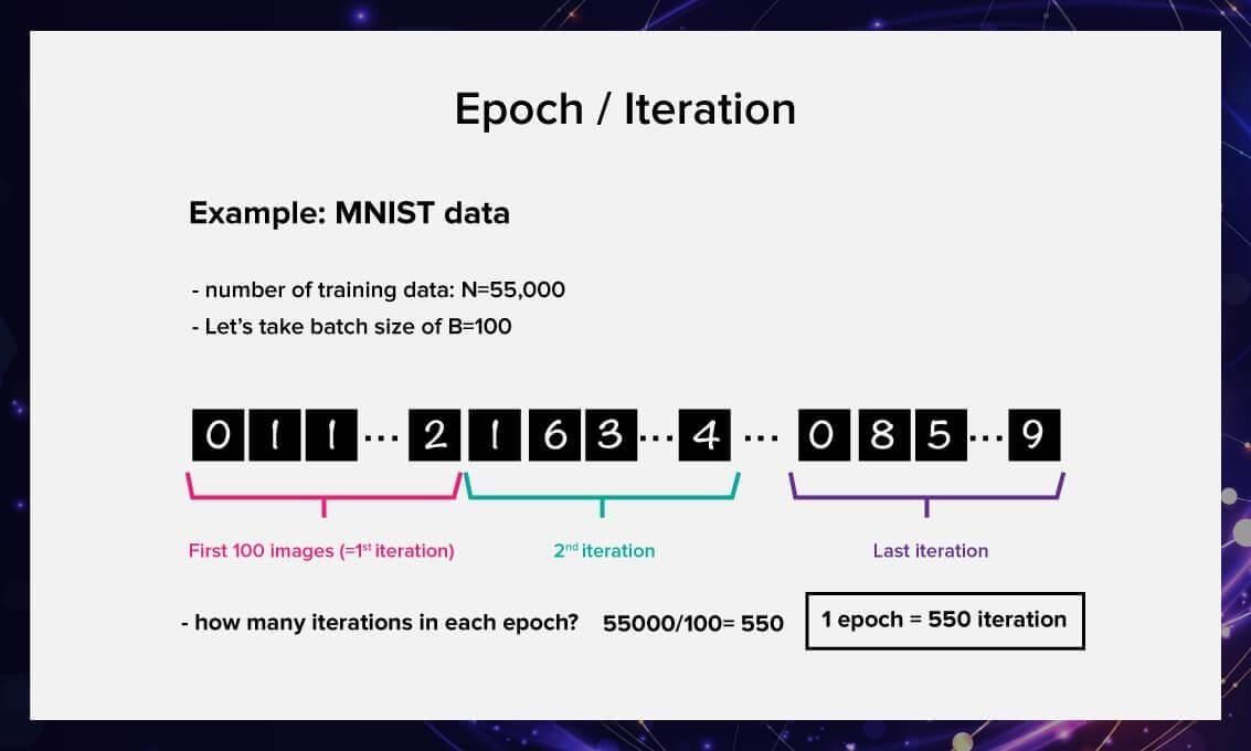
- If we train for one epoch, the model sees each training sample exactly once.
- If we train for multiple epochs, the model repeatedly sees the same data and continuously updates its weights to improve performance.
Choosing the Number of Epochs
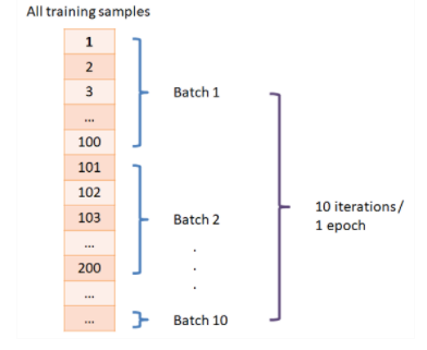
- Too Few Epochs → The model may underfit, meaning it has not learned enough patterns from the data.
- Too Many Epochs → The model may overfit, meaning it memorizes the training data but generalizes poorly to new data.
- The optimal number of epochs is typically determined using early stopping, which monitors validation loss and stops training when the loss starts increasing (a sign of overfitting).
TensorFlow Implementation
model.fit(X_train, y_train, epochs=50, batch_size=32, validation_data=(X_val, y_val))
Batch Size
Instead of feeding the entire dataset into the model at once, training is performed in smaller subsets called batches.
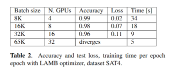
Key Concepts:
- Batch Size: The number of training samples processed before updating the model’s weights.
- Iteration: One update of the model’s weights after processing a batch.
- Steps Per Epoch: If we have
Ntraining samples and batch sizeB, then the number of steps per epoch is N/B.
Choosing Batch Size
- Small Batch Sizes (e.g., 16, 32):
- Require less memory.
- Provide noisy but effective updates (better generalization).
- Large Batch Sizes (e.g., 256, 512, 1024):
- Require more memory.
- Lead to smoother but potentially less generalized updates.
TensorFlow Implementation
model.fit(X_train, y_train, epochs=20, batch_size=64)
Validation Data
A validation set is a separate portion of the dataset that is not used for training. It helps monitor the model’s performance and detect overfitting.
Differences Between Training, Validation, and Test Data:
| Data Type | Purpose |
|---|---|
| Training Set | Used for updating model weights during training. |
| Validation Set | Used to tune hyperparameters and detect overfitting. |
| Test Set | Used to evaluate final model performance on unseen data. |
How to Split Data:
A common split is 80% training, 10% validation, 10% test, but this can vary based on dataset size.
TensorFlow Implementation
from sklearn.model_selection import train_test_split
X_train, X_val, y_train, y_val = train_test_split(X, y, test_size=0.2, random_state=42)
model.fit(X_train, y_train, epochs=30, batch_size=32, validation_data=(X_val, y_val))
Activation Functions
1. Why Do We Need Activation Functions?
Without an activation function, a neural network with multiple layers behaves like a single-layer linear model because:
$$ f(x) = Wx + b $$
is just a linear transformation. Activation functions introduce non-linearity, allowing the network to learn complex patterns.
If we do not apply non-linearity, no matter how many layers we stack, the final output remains a linear function of the input. Activation functions solve this by enabling the model to approximate complex, non-linear relationships.
2. Common Activation Functions
Sigmoid (Logistic Function)
$$ \sigma(x) = \frac{1}{1 + e^{-x}} $$
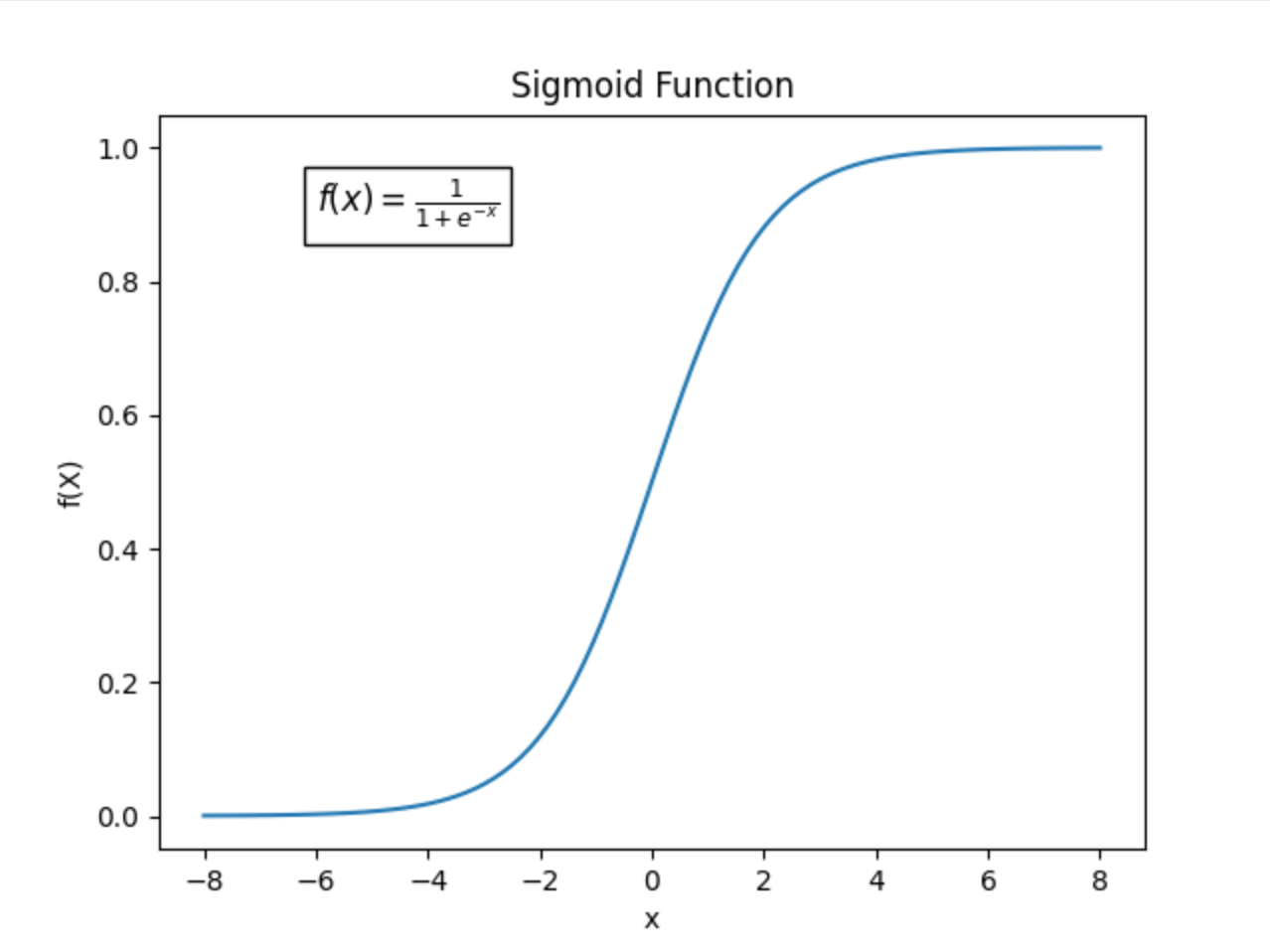
- Range: (0, 1)
- Used in: Binary classification problems
- Pros: Outputs can be interpreted as probabilities.
- Cons: Vanishing gradients for very large or very small values of ( x ), making training slow.
ReLU (Rectified Linear Unit)
$$ f(x) = \max(0, x) $$
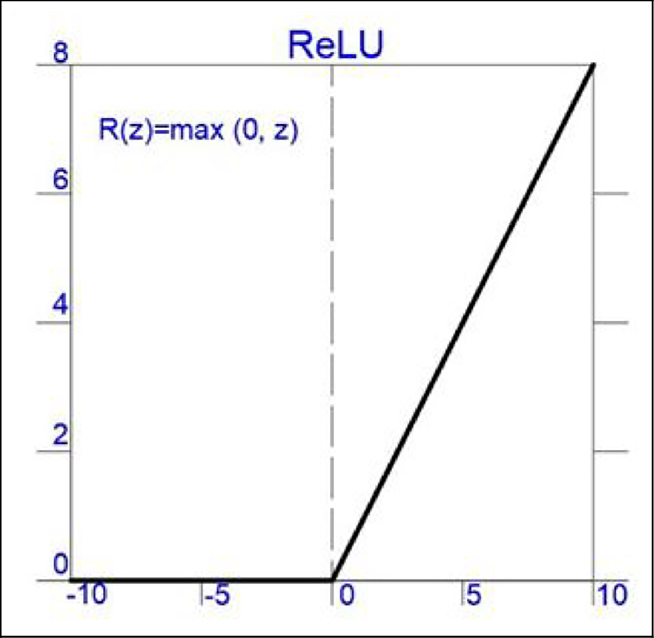
- Range: [0, ∞)
- Used in: Hidden layers of deep neural networks.
- Pros: Helps with gradient flow and avoids vanishing gradients.
- Cons: Can suffer from dying ReLU problem (where neurons output 0 and stop learning if input is negative).
Leaky ReLU
$$ f(x) = \max(0.01x, x) $$
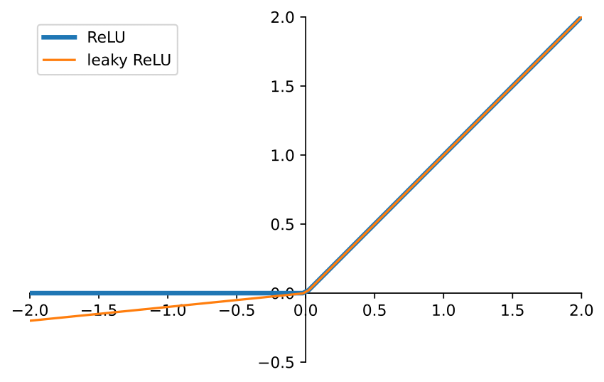
- Range: (-∞, ∞)
- Used in: Hidden layers as an alternative to ReLU.
- Pros: Prevents the dying ReLU problem.
- Cons: Small negative slope may still lead to slow learning.
Softmax
$$ \sigma(xi) = \frac{e^{x_i}}{\sum{j} e^{x_j}} $$
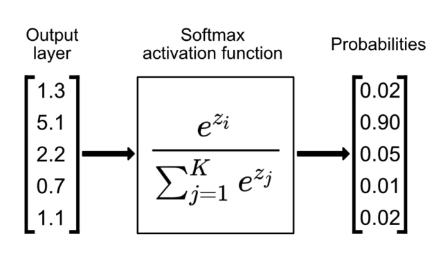
- Used in: Multi-class classification (output layer).
- Pros: Outputs a probability distribution (each class gets a probability between 0 and 1, summing to 1).
- Cons: Can lead to numerical instability when exponentiating large numbers.
Linear Activation
$$ f(x) = x $$
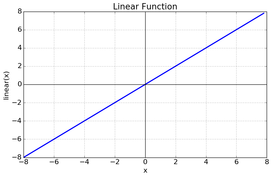
- Used in: Regression problems (output layer).
- Pros: No constraints on output values.
- Cons: Not useful for classification since it doesn’t map values to a specific range.
3. Choosing the Right Activation Function
| Layer | Recommended Activation Function | Explanation |
|---|---|---|
| Hidden Layers | ReLU (or Leaky ReLU if ReLU is dying) | Helps with deep networks by maintaining gradient flow |
| Output Layer (Binary Classification) | Sigmoid | Outputs probabilities for two-class classification |
| Output Layer (Multi-Class Classification) | Softmax | Converts logits into probability distributions |
| Output Layer (Regression) | Linear | Directly outputs numerical values |
Softmax vs. Sigmoid: Key Differences
- Sigmoid is mainly used for binary classification, mapping values to (0,1), which can be interpreted as class probabilities.
- Softmax is used for multi-class classification, producing a probability distribution over multiple classes.
If you use sigmoid for multi-class problems, each output node will act independently, making it difficult to ensure they sum to 1. Softmax ensures that outputs sum to 1, providing a clearer probabilistic interpretation.
Improved Implementation of Softmax
Why Use Linear Instead of Softmax in the Output Layer?
When implementing a neural network for classification, we often pass logits (raw outputs) directly into the loss function instead of applying softmax explicitly.
Mathematically, if we apply softmax explicitly:
$$ L = - \sum y_i \log(\sigma(z_i)) $$
where ( \sigma(z) ) is the softmax function.
However, if we pass raw logits (without softmax) into the cross-entropy loss function, TensorFlow applies the log-softmax trick internally:
$$ L = - \sum y_i z_i + \log \sum e^{z_i} $$
This avoids computing large exponentials, improving numerical stability and reducing computation cost.
TensorFlow Implementation
Instead of:
model = tf.keras.Sequential([
tf.keras.layers.Dense(128, activation='relu'),
tf.keras.layers.Dense(64, activation='relu'),
tf.keras.layers.Dense(10, activation='softmax') # Explicit softmax
])
model.compile(loss=tf.keras.losses.SparseCategoricalCrossentropy(), optimizer='adam')
Use:
model = tf.keras.Sequential([
tf.keras.layers.Dense(128, activation='relu'),
tf.keras.layers.Dense(64, activation='relu'),
tf.keras.layers.Dense(10) # No activation here!
])
model.compile(loss=tf.keras.losses.SparseCategoricalCrossentropy(from_logits=True), optimizer='adam')
This allows TensorFlow to handle softmax internally, avoiding unnecessary computation and improving numerical precision.
Optimizers and Layer Types
- Optimizers in Deep Learning
- Choosing the Right Optimizer
- Gradient Descent (GD)
- Stochastic Gradient Descent (SGD)
- Stochastic Gradient Descent with Momentum (SGD-Momentum)
- Mini-Batch Gradient Descent
- Adagrad (Adaptive Gradient Descent)
- RMSprop (Root Mean Square Propagation)
- AdaDelta
- Adam (Adaptive Moment Estimation)
- Hands-on Optimizers
- Table Analysis
- Conclusion
- Additional Layer Types in Neural Networks
Optimizers in Deep Learning
Optimizers play a crucial role in training deep learning models by adjusting the model parameters to minimize the loss function. Different optimization algorithms have been developed to improve convergence speed, accuracy, and stability. In this article, we explore various optimizers used in deep learning, their mathematical formulations, and practical implementations.
Choosing the Right Optimizer
Choosing the right optimizer depends on several factors, including:
- The nature of the dataset
- The complexity of the model
- The presence of noisy gradients
- The required computational efficiency
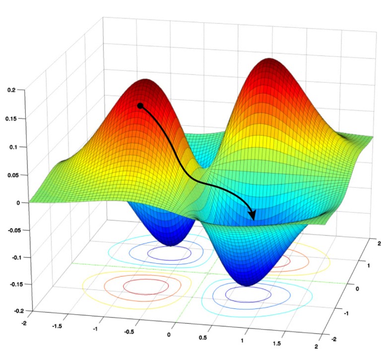
Below, we examine different types of optimizers along with their mathematical formulations.
Gradient Descent (GD)
Mathematical Formulation
Gradient Descent updates model parameters $ \theta $ iteratively using the gradient of the loss function $ J(\theta) $:
$$ \theta = \theta - \alpha \nabla J(\theta) $$
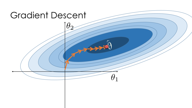
where:
- $ \alpha $ is the learning rate
- $ \nabla J(\theta) $ is the gradient of the loss function
Characteristics
- Computes gradient over the entire dataset
- Slow for large datasets
- Prone to getting stuck in local minima
Stochastic Gradient Descent (SGD)
Gradient descent struggles with massive datasets, making stochastic gradient descent (SGD) a better alternative. Unlike standard gradient descent, SGD updates model parameters using small, randomly selected data batches, improving computational efficiency.
SGD initializes parameters $𝑤$ and learning rate $\alpha$, then shuffles data at each iteration, updating based on mini-batches. This introduces noise, requiring more iterations to converge, but still reduces overall computation time compared to full-batch gradient descent.
For large datasets where speed matters, SGD is preferred over batch gradient descent.
Mathematical Formulation
Instead of computing the gradient over the entire dataset, SGD updates $ \theta $ using a single data point:
$$ \theta = \theta - \alpha \nabla J(\theta; x_i, y_i) $$
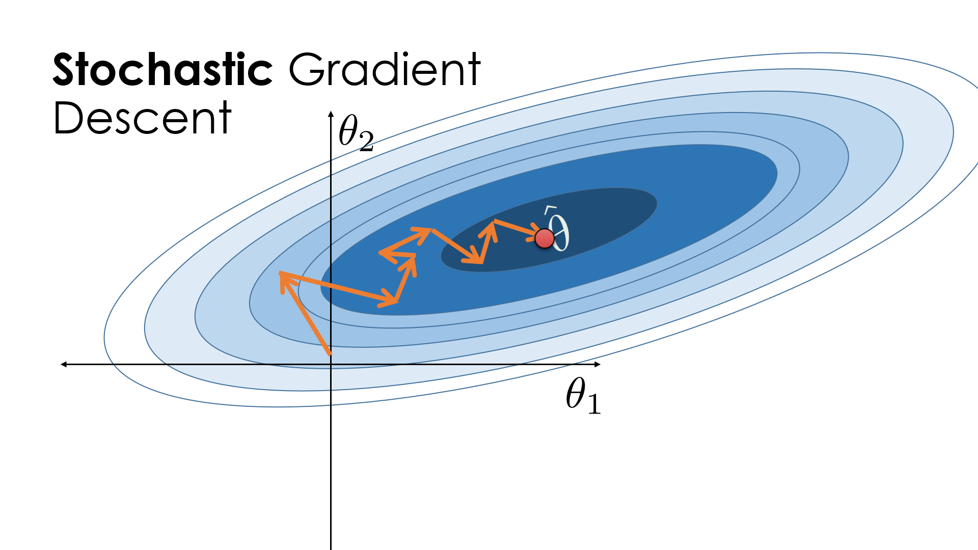
where $ x_i, y_i $ is a single training example.
Characteristics
- Faster than full-batch gradient descent
- High variance in updates
- Introduces noise, which can help escape local minima
Stochastic Gradient Descent with Momentum (SGD-Momentum)
SGD follows a noisy optimization path, requiring more iterations and longer computation time. To speed up convergence, SGD with momentum is used.
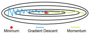
Momentum helps stabilize updates by adding a fraction of the previous update to the current one, reducing oscillations and accelerating convergence. However, a high momentum term requires lowering the learning rate to avoid overshooting the optimal minimum.
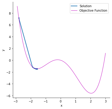
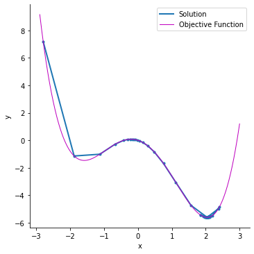
While momentum improves speed, too much momentum can cause instability and poor accuracy. Proper tuning is essential for effective optimization.
Mathematical Formulation
Momentum helps accelerate SGD by maintaining a velocity term:
$$ v_t = \beta v_{t-1} + (1 - \beta) \nabla J(\theta) $$
$$ \theta = \theta - \alpha v_t $$
where:
- $ v_t $ is the momentum term
- $ \beta $ is a momentum coefficient (typically 0.9)
Characteristics
- Reduces oscillations
- Faster convergence
Mini-Batch Gradient Descent
Mini-batch gradient descent optimizes training by using a subset of data instead of the entire dataset, reducing the number of iterations needed. This makes it faster than both stochastic and batch gradient descent while being more efficient and memory-friendly.
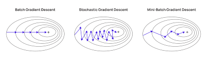
Key Advantages
- Balances speed and accuracy by reducing noise compared to SGD but keeping updates more dynamic than batch gradient descent.
- Doesn’t require loading all data into memory, improving implementation efficiency.
Limitations
- Requires tuning the mini-batch size (typically 32) for optimal accuracy.
- May lead to poor final accuracy in some cases, requiring alternative approaches.
Mathematical Formulation
$$ \theta = \theta - \alpha \frac{1}{m} \sum\limits_{i=1}^{m} \nabla J(\theta; x_i, y_i) $$
Instead of updating with the entire dataset or a single example, mini-batch GD uses a small batch of $ m $ samples:
Adagrad (Adaptive Gradient Descent)
Adagrad differs from other gradient descent algorithms by using a unique learning rate for each iteration, adjusting based on parameter changes. Larger parameter updates lead to smaller learning rate adjustments, making it effective for datasets with both sparse and dense features.
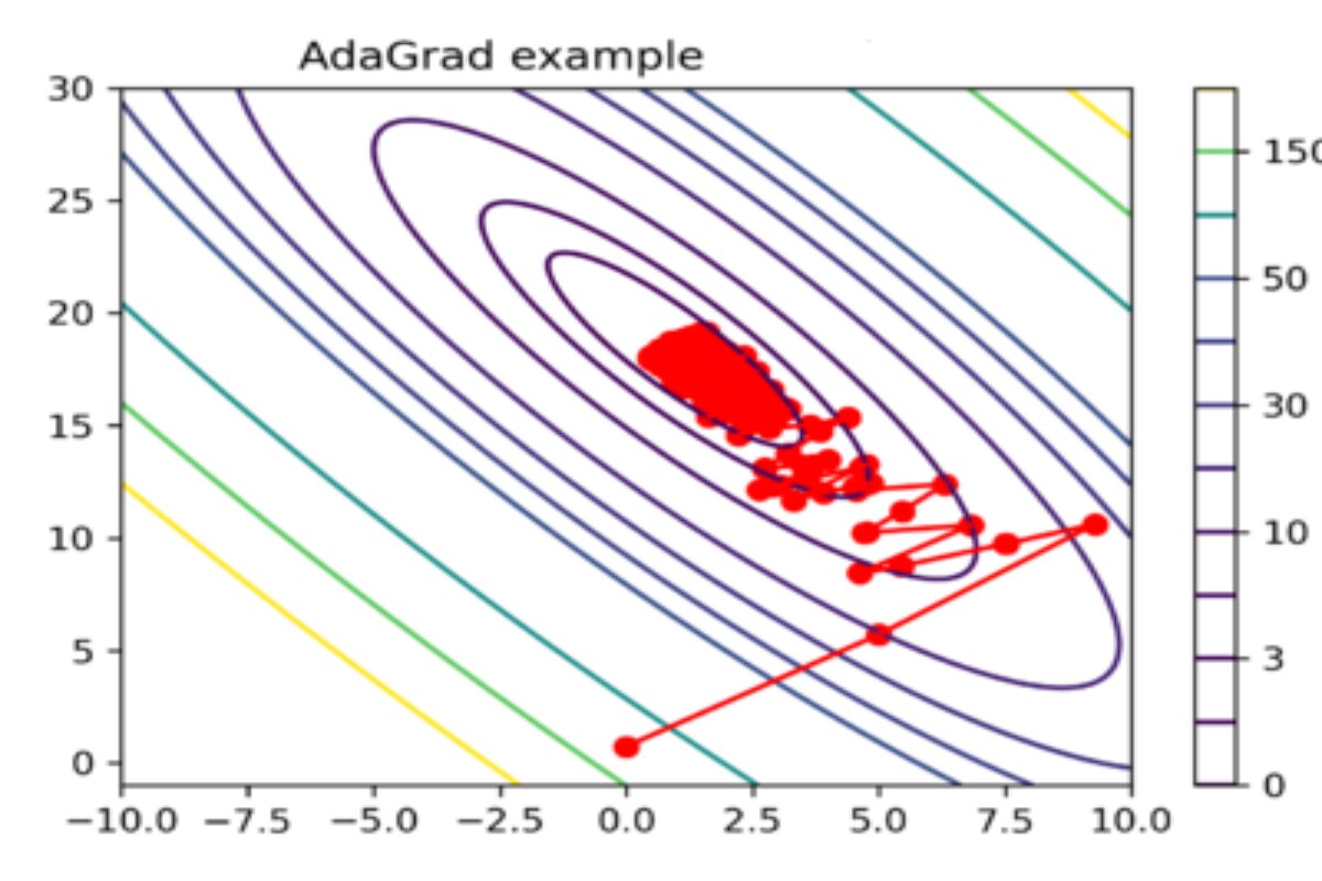
Key Advantages
- Eliminates manual learning rate tuning by adapting automatically.
- Faster convergence compared to standard gradient descent methods.
Limitations
- Aggressively reduces the learning rate over time, which can slow learning and harm accuracy.
- The accumulation of squared gradients in the denominator causes the learning rate to become too small, limiting further model improvements.
Mathematical Formulation
Adagrad adapts learning rates for each parameter:
$$ \theta = \theta - \frac{\alpha}{\sqrt{G*{t} + \epsilon}} \nabla J(\theta) $$
where $ G_t $ accumulates past squared gradients:
$$ G_t = G_{t-1} + \nabla J(\theta)^2 $$
Characteristics
- Suitable for sparse data
- Learning rate decreases over time
RMSprop (Root Mean Square Propagation)
RMSProp improves stability by adapting step sizes per weight, preventing large gradient fluctuations. It maintains a moving average of squared gradients to adjust learning rates dynamically.
Mathematical Formulation
$$ G_t = \beta G_{t-1} + (1 - \beta) \nabla J(\theta)^2 $$
$$ \theta = \theta - \frac{\alpha}{\sqrt{G_{t} + \epsilon}} \nabla J(\theta) $$
Pros
- Faster convergence with smoother updates.
- Less tuning than other gradient descent variants.
- More stable than Adagrad by preventing extreme learning rate decay.
Cons
- Requires manual learning rate tuning, and default values may not always be optimal.
AdaDelta
Mathematical Formulation
AdaDelta modifies Adagrad by using an exponentially decaying average of past squared gradients:
$$ \Delta \theta_t = - \frac{\sqrt{E[\Delta \theta^2] + \epsilon}}{\sqrt{E[g^2] + \epsilon}} g_t $$
where $ E[\cdot] $ is the moving average.
Characteristics
- Addresses diminishing learning rates in Adagrad
- No need to manually set a learning rate
Adam (Adaptive Moment Estimation)
Adam (Adaptive Moment Estimation) is a widely used deep learning optimizer that extends SGD by dynamically adjusting learning rates for each weight. It combines AdaGrad and RMSProp to balance adaptive learning rates and stable updates.
Mathematical Formulation
Adam combines momentum and RMSprop:
$$ m_t = \beta_1 m_{t-1} + (1 - \beta*1) \nabla J(\theta) $$
$$ v_t = \beta_2 v_{t-1} + (1 - \beta_2) \nabla J(\theta)^2 $$
$$ \theta = \theta - \alpha \frac{\hat{m_t}}{\sqrt{\hat{v_t}} + \epsilon} $$
where $ \hat{m_t} $ and $ \hat{v_t} $ are bias-corrected estimates.
Key Features
- Uses first (mean) and second (variance) moments of gradients.
- Faster convergence with minimal tuning.
- Low memory usage and efficient computation.
Downsides
- Prioritizes speed over generalization, making SGD better for some cases.
- May not always be ideal for every dataset.
Adam is the default choice for many deep learning tasks but should be selected based on the dataset and training requirements.
Hands-on Optimizers
Import Necessary Libraries
import keras
from keras.datasets import mnist
from keras.models import Sequential
from keras.layers import Dense, Dropout, Flatten
from keras.layers import Conv2D, MaxPooling2D
from keras import backend as K
(x_train, y_train), (x_test, y_test) = mnist.load_data()
print(x_train.shape, y_train.shape)
Load the Dataset
x_train= x_train.reshape(x_train.shape[0],28,28,1)
x_test= x_test.reshape(x_test.shape[0],28,28,1)
input_shape=(28,28,1)
y_train=keras.utils.to_categorical(y_train)#,num_classes=)
y_test=keras.utils.to_categorical(y_test)#, num_classes)
x_train= x_train.astype('float32')
x_test= x_test.astype('float32')
x_train /= 255
x_test /=255
Build the Model
batch_size=64
num_classes=10
epochs=10
def build_model(optimizer):
model=Sequential()
model.add(Conv2D(32,kernel_size=(3,3),activation='relu',input_shape=input_shape))
model.add(MaxPooling2D(pool_size=(2,2)))
model.add(Dropout(0.25))
model.add(Flatten())
model.add(Dense(256, activation='relu'))
model.add(Dropout(0.5))
model.add(Dense(num_classes, activation='softmax'))
model.compile(loss=keras.losses.categorical_crossentropy, optimizer= optimizer, metrics=['accuracy'])
return model
Train the Model
optimizers = ['Adadelta', 'Adagrad', 'Adam', 'RMSprop', 'SGD']
for i in optimizers:
model = build_model(i)
hist=model.fit(x_train, y_train, batch_size=batch_size, epochs=epochs, verbose=1, validation_data=(x_test,y_test))
Table Analysis
| Optimizer | Epoch 1 (Val Acc | Val Loss) | Epoch 5 (Val Acc | Val Loss) | Epoch 10 (Val Acc | Val Loss) | Total Time |
|---|---|---|---|---|---|---|---|
| Adadelta | .4612 | 2.2474 | .7776 | 1.6943 | .8375 | 0.9026 | 8:02 min |
| Adagrad | .8411 | .7804 | .9133 | .3194 | .9286 | 0.2519 | 7:33 min |
| Adam | .9772 | .0701 | .9884 | .0344 | .9908 | .0297 | 7:20 min |
| RMSprop | .9783 | .0712 | .9846 | .0484 | .9857 | .0501 | 10:01 min |
| SGD with momentum | .9168 | .2929 | .9585 | .1421 | .9697 | .1008 | 7:04 min |
| SGD | .9124 | .3157 | .9569 | 1.451 | .9693 | .1040 | 6:42 min |
The above table shows the validation accuracy and loss at different epochs. It also contains the total time that the model took to run on 10 epochs for each optimizer. From the above table, we can make the following analysis.
- The adam optimizer shows the best accuracy in a satisfactory amount of time.
- RMSprop shows similar accuracy to that of Adam but with a comparatively much larger computation time.
- Surprisingly, the SGD algorithm took the least time to train and produced good results as well. But to reach the accuracy of the Adam optimizer, SGD will require more iterations, and hence the computation time will increase.
- SGD with momentum shows similar accuracy to SGD with unexpectedly larger computation time. This means the value of momentum taken needs to be optimized.
- Adadelta shows poor results both with accuracy and computation time.
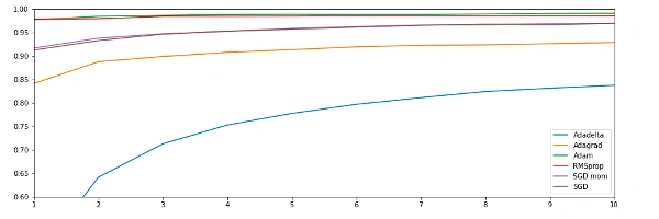
You can analyze the accuracy of each optimizer with each epoch from the above graph.
Conclusion
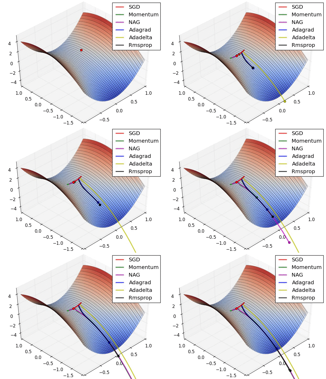
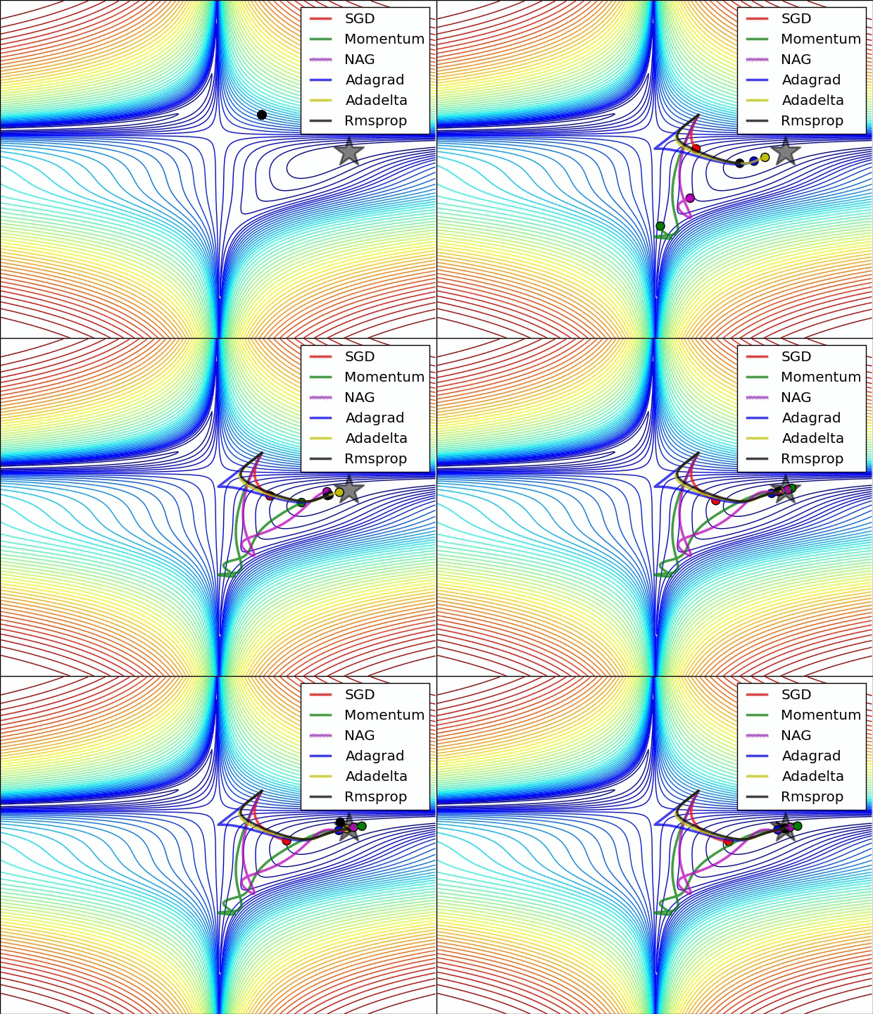
Different optimizers offer unique advantages based on the dataset and model architecture. While SGD is the simplest, Adam is often preferred for deep learning tasks due to its adaptive learning rate and momentum.
By understanding these optimizers, you can fine-tune deep learning models for optimal performance!
Additional Layer Types in Neural Networks
In deep learning, different layer types serve distinct purposes, helping neural networks learn complex representations. This section explores various layer types, their mathematical foundations, and practical implementations.
Dense Layer (Fully Connected Layer)
A Dense layer is a fundamental layer where each neuron is connected to every neuron in the previous layer.
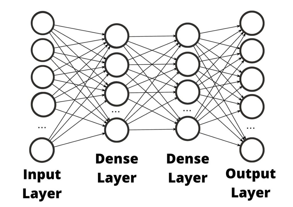
Mathematical Representation:
Given an input vector $ x $ of size $ n $, weights $ W $ of size $ m \times n $, and bias $ b $ of size $ m $, the output $ y $ is calculated as:
$$ y = f(Wx + b) $$
where $ f $ is an activation function such as ReLU, Sigmoid, or Softmax.
Implementation in TensorFlow:
import tensorflow as tf
from tensorflow.keras.models import Sequential
from tensorflow.keras.layers import Dense
model = Sequential([
Dense(64, activation='relu', input_shape=(100,)),
Dense(32, activation='relu'),
Dense(10, activation='softmax')
])
model.summary()
Convolutional Layer (Conv2D)
A Convolutional layer is used in image processing, applying filters (kernels) to extract features from input images.
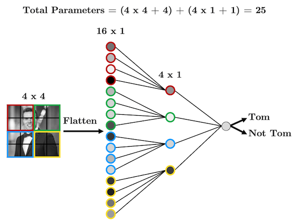
Mathematical Representation:
For an input image $ I $ and a filter $ K $, the convolution operation is defined as:
$$ S(i, j) = \sum_m \sum_n I(i+m, j+n) K(m, n) $$
Implementation in TensorFlow:
from tensorflow.keras.layers import Conv2D
model = Sequential([
Conv2D(32, kernel_size=(3,3), activation='relu', input_shape=(28,28,1)),
Conv2D(64, kernel_size=(3,3), activation='relu'),
])
model.summary()
Pooling Layer (MaxPooling & AveragePooling)
Pooling layers reduce dimensionality while preserving important features.
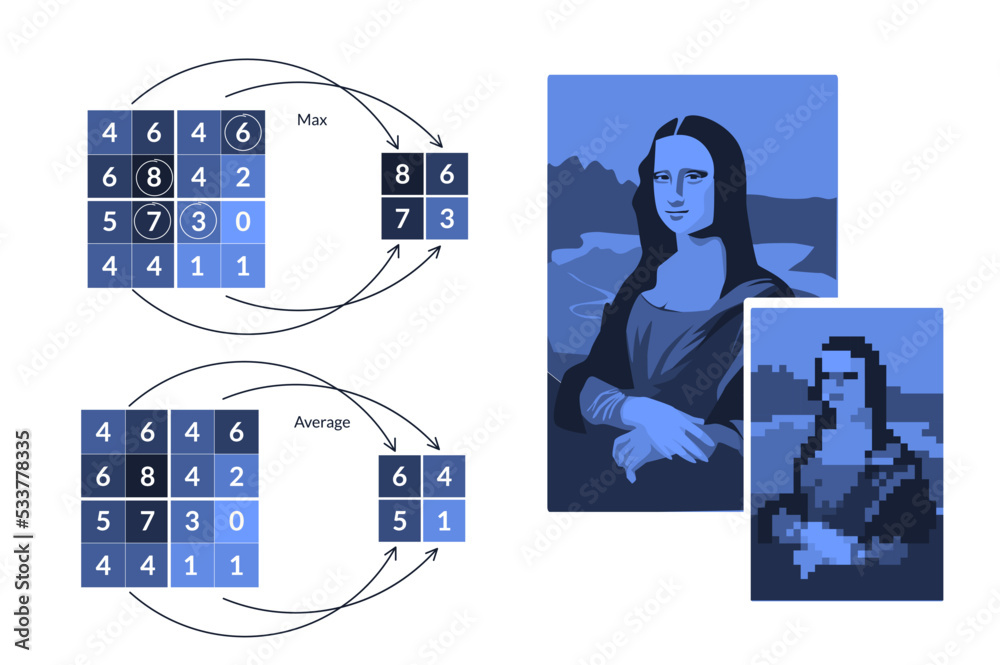
Max Pooling:
$$ S(i, j) = \max (I_{region}) $$
Average Pooling:
$$ S(i, j) = \frac{1}{N} \sum I_{region} $$
Implementation:
from tensorflow.keras.layers import MaxPooling2D, AveragePooling2D
model = Sequential([
MaxPooling2D(pool_size=(2,2)),
AveragePooling2D(pool_size=(2,2))
])
model.summary()
Recurrent Layer (RNN, LSTM, GRU)
Recurrent layers process sequential data by maintaining memory of past inputs.
RNN Mathematical Model:
$$ h_t = f(W_h h_{t-1} + W_x x_t + b) $$
LSTM Update Equations:
$$ i_t = \sigma(W_i x_t + U_i h_{t-1} + b_i) $$
$$ f_t = \sigma(W_f x_t + U_f h_{t-1} + b_f) $$
$$ c_t = f_t c_{t-1} + i_t \tanh(W_c x_t + U_c h_{t-1} + b_c) $$
Implementation:
from tensorflow.keras.layers import SimpleRNN, LSTM, GRU
model = Sequential([
LSTM(64, return_sequences=True, input_shape=(100, 10)),
GRU(32)
])
model.summary()
Dropout Layer
The Dropout layer randomly sets a fraction of input units to 0 to prevent overfitting.
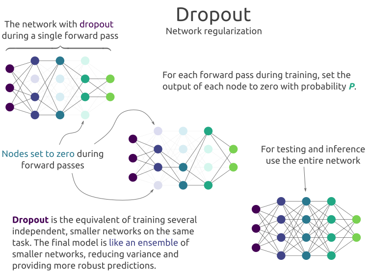
Mathematical Explanation:
During training, for each neuron, the probability of being kept is $ p $:
$$ y = \frac{1}{p} f(Wx + b) \quad \text{if neuron is kept, else } y = 0 $$
Implementation:
from tensorflow.keras.layers import Dropout
model = Sequential([
Dense(128, activation='relu'),
Dropout(0.5),
Dense(64, activation='relu'),
Dropout(0.3),
Dense(10, activation='softmax')
])
model.summary()
Comparison Table
| Layer Type | Purpose | Typical Use Case |
|---|---|---|
| Dense | Fully connected layer | General deep learning models |
| Conv2D | Feature extraction | Image processing |
| Pooling | Downsampling | CNNs to reduce size |
| RNN | Sequential processing | Time-series, NLP |
| LSTM/GRU | Long-term memory retention | Language models |
| Dropout | Overfitting prevention | Regularization in deep networks |
Conclusion
Understanding different types of layers is crucial in designing effective deep learning models. Choosing the right layers based on the data type and problem domain significantly impacts model performance. Experimenting with combinations of these layers is key to optimizing results.
Model Evaluation, Selection, and Improvement
- Evaluating a Model
- Model Selection and Training/Validation/Test Sets
- Diagnosing Bias and Variance
- Regularization and Bias-Variance Tradeoff
- Establishing a Baseline Level of Performance
- Iterative Loop of ML Development
- Adding Data: Data Augmentation & Synthesis
- Transfer Learning: Using Data from a Different Task
- Error Metrics for Skewed Datasets
Evaluating a Model
A metric is a numerical measure used to assess the performance of a model on a given dataset. Metrics help quantify how well a model is making predictions and whether it meets the desired objectives. The choice of metric depends on the nature of the problem:
- For classification tasks, we often measure how accurately a model assigns labels.
- For regression tasks, we evaluate how close the model’s predictions are to actual values.
- In other domains like natural language processing (NLP) or computer vision, specialized metrics are used.
However, a high metric value does not always mean a model is truly effective. For example:
- In an imbalanced dataset, accuracy might be misleading. A model predicting the majority class 100% of the time can have high accuracy but perform poorly overall.
- A regression model with a low mean squared error (MSE) might still fail in real-world applications if it makes large errors in critical cases.
Key Metrics for Model Evaluation
Classification Metrics
- Accuracy: Measures the percentage of correctly predicted instances.
- Precision: The fraction of true positive predictions among all positive predictions.
- Recall: The fraction of actual positives correctly identified.
- F1-score: The harmonic mean of precision and recall, useful for imbalanced datasets.
- ROC-AUC (Receiver Operating Characteristic - Area Under Curve): Evaluates the model’s ability to distinguish between classes.
Regression Metrics
- Mean Squared Error (MSE): Measures the average squared difference between predicted and actual values.
- Mean Absolute Error (MAE): Measures the average absolute difference.
- R-squared (R²): Indicates how well the model explains variance in the data.
Other Metrics
- Log loss: Used for probabilistic classification models.
- BLEU score: Measures similarity in NLP tasks.
- Intersection over Union (IoU): Used in object detection to measure overlap between predicted and actual bounding boxes.
Choosing the Right Metric
Suppose we are building a spam classifier. If 99% of emails are non-spam, a naive model predicting “not spam” for all emails will have 99% accuracy but be completely useless. In this case, precision and recall are more meaningful metrics because they tell us how well the model detects actual spam emails without too many false positives.
Thus, choosing the right metric is just as important as achieving a high score. A well-performing model is one that aligns with the real-world objective of the task.
Model Selection and Training/Validation/Test Sets
Selecting the right model is essential for achieving high performance on unseen data. A model that performs well on training data but poorly on new data is overfitting, while a model that is too simple may underfit. To properly evaluate a model and fine-tune its performance, we split the dataset into three key subsets:
Training Set
The training set is the portion of the data used to train the machine learning model. The model learns patterns from this data by adjusting its internal parameters. However, evaluating the model only on the training set is misleading because the model might memorize the data instead of generalizing from it.
Validation Set
The validation set is a separate portion of the dataset that is used to tune hyperparameters and select the best model architecture. Hyperparameters are external configuration settings that are not learned by the model but instead set manually or through automated search methods. Examples of hyperparameters include:
- Learning rate
- Number of hidden layers in a neural network
- Regularization parameters (L1, L2)
- Batch size
By testing different hyperparameter values on the validation set, we can find the combination that leads to the best generalization performance. However, if the validation set is too small or used excessively for tuning, the model might start overfitting to it.
Test Set
The test set is used only once, after model training and hyperparameter tuning, to evaluate the final model’s performance. The test set should remain completely unseen during training and validation to provide an unbiased estimate of how the model will perform on real-world data.
Cross-Validation
Cross-validation is a technique to make better use of available data and improve model selection. Instead of relying on a single validation set, we divide the dataset into multiple subsets and perform training and validation multiple times. The most common approach is k-fold cross-validation, which works as follows:
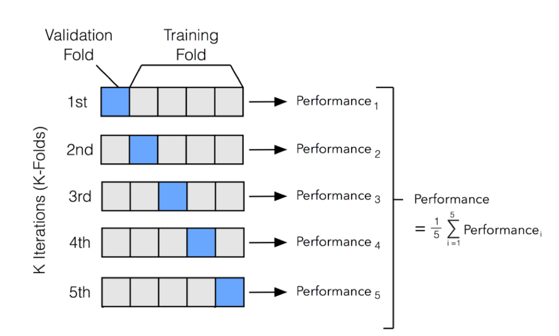
- The dataset is divided into k equal-sized folds.
- The model is trained on k-1 folds and validated on the remaining one.
- This process is repeated k times, with each fold serving as the validation set once.
- The final performance metric is the average of all validation scores.
For example, in 5-fold cross-validation, the dataset is split into 5 parts. The model is trained on 4 parts and validated on the remaining one, and this process repeats until each part has been used as a validation set once. This reduces the risk of selecting a model that performs well on just one specific validation set but poorly on unseen data.
Cross-validation is especially useful when working with small datasets since it allows more efficient use of data. However, it can be computationally expensive, especially for deep learning models, where training is time-consuming.
By using training, validation, and test sets appropriately—along with cross-validation where necessary—we can make informed decisions about model selection and ensure good generalization to new data.
Diagnosing Bias and Variance
Bias and variance are two key factors that determine a model’s ability to generalize to unseen data. To understand these concepts, let’s analyze the simple linear model:
$$ f(x) = wx + b $$
A well-performing model should generalize well, meaning it captures the essential patterns in the data without memorizing noise. Let’s break this down using the equation.
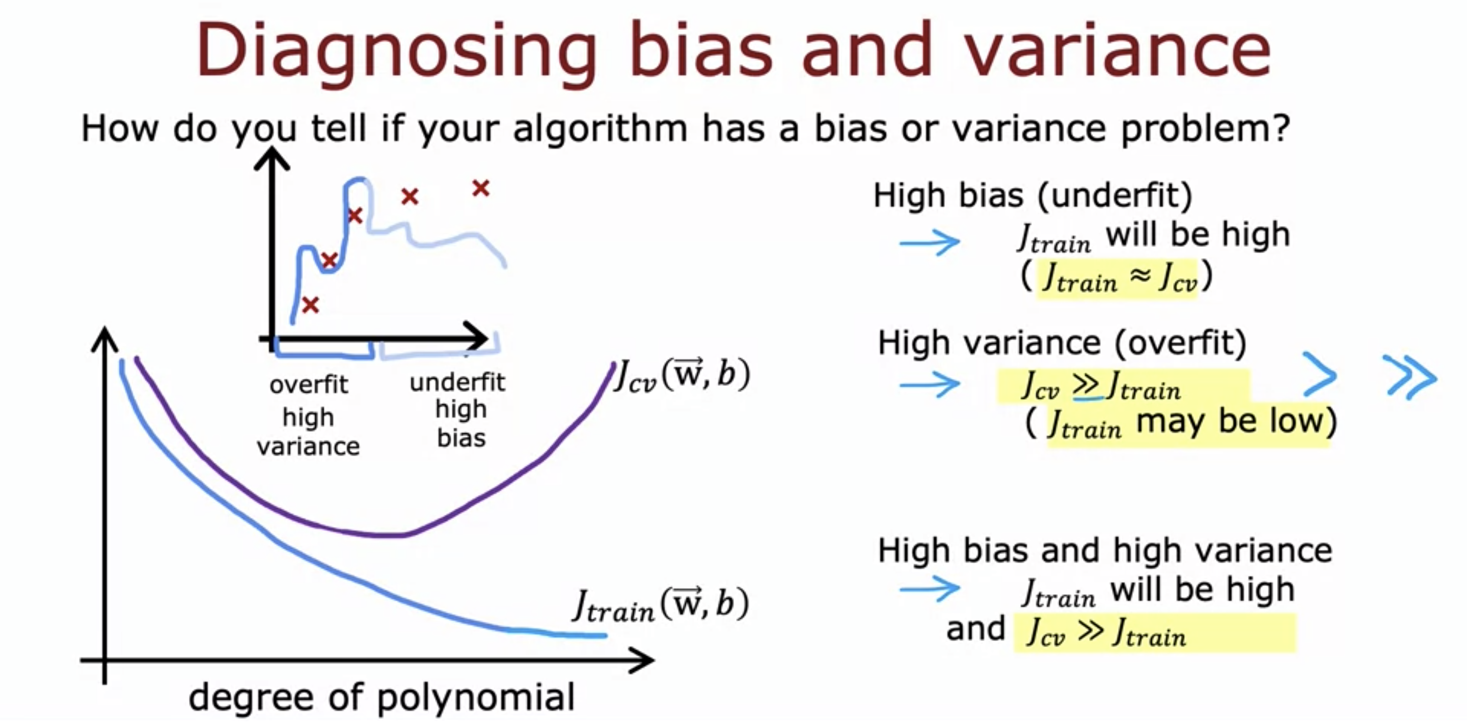
| Issue | Description | Effects | Impact of More Data |
|---|---|---|---|
| High Bias (Underfitting) | Model is too simple and cannot capture underlying patterns. | - Poor performance on both training and test sets. - Model is too simplistic. | Increasing training data does not improve performance. |
| High Variance (Overfitting) | Model is too complex and memorizes training data, including noise. | - Training error is very low, but test error is high. - Model learns noise instead of actual patterns. | Increasing training data can help generalization. |
Regularization and Bias-Variance Tradeoff
To prevent overfitting, we introduce regularization, which penalizes large weights.
The regularized loss function:
$$ J(w) = \text{Loss}(w) + \lambda \sum_{i} \phi(w_i) $$
where:
- $ \text{Loss}(w) $ is the original loss function (e.g., Mean Squared Error),
- $ \lambda $ is the regularization strength,
- $ \phi(w) $ is the penalty term (L1 or L2).
Effect of Regularization
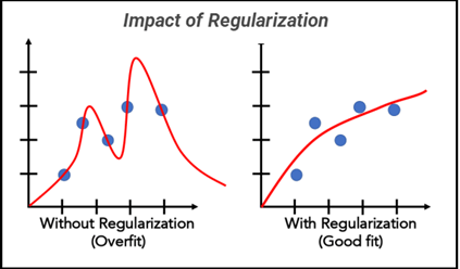
- If $ \lambda $ is too low, the model can overfit ($ w $ values become large).
- If $ \lambda $ is too high, the model becomes too simple ($ w $ values shrink too much).
- The ideal $ \lambda $ value balances bias and variance.
Establishing a Baseline Level of Performance
A baseline model helps measure improvement. Common baselines include:
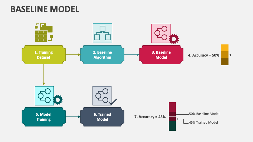
- Random classifiers (for classification tasks)
- Mean predictions (for regression tasks)
- Simple heuristic-based methods
A model must outperform the baseline to be considered useful.
Iterative Loop of ML Development
Machine learning development follows an iterative cycle:
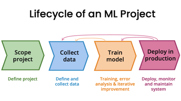
- Train a baseline model.
- Diagnose bias/variance errors.
- Adjust model complexity, regularization, or data strategy.
- Repeat until performance is satisfactory.
Adding Data: Data Augmentation & Synthesis
One of the most effective ways to improve a model’s generalization ability is by increasing the amount of training data. More data helps the model learn patterns that are not specific to the training set, reducing overfitting and improving robustness.
Data Augmentation
Data Augmentation refers to artificially increasing the size of the training dataset by applying transformations to existing data. It is particularly useful in fields like computer vision and NLP, where collecting labeled data is expensive and time-consuming.
Common Data Augmentation Techniques
-
Image Data Augmentation (Used in deep learning for computer vision tasks):
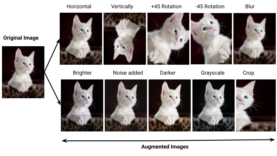
- Rotation: Rotating images by small degrees to simulate different perspectives.
- Cropping: Randomly cropping parts of the image to focus on different areas.
- Flipping: Horizontally or vertically flipping images.
- Scaling: Resizing images while maintaining aspect ratios.
- Brightness/Contrast Adjustments: Modifying brightness and contrast to simulate lighting variations.
- Noise Injection: Adding Gaussian noise to simulate different sensor conditions.
Example in TensorFlow/Keras:
from tensorflow.keras.preprocessing.image import ImageDataGenerator datagen = ImageDataGenerator( rotation_range=20, width_shift_range=0.1, height_shift_range=0.1, horizontal_flip=True, brightness_range=[0.8, 1.2] ) augmented_images = datagen.flow(x_train, y_train, batch_size=32) -
Text Data Augmentation (Used in NLP models):
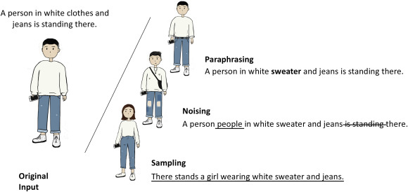
-
Synonym Replacement: Replacing words with their synonyms.
-
Random Insertion: Adding random words from the vocabulary.
-
Back Translation: Translating text to another language and back to introduce variation.
-
Sentence Shuffling: Reordering words or sentences slightly.
Example using
nlpaug:
import nlpaug.augmenter.word as naw aug = naw.SynonymAug(aug_src='wordnet') text = "Deep learning models require large amounts of data." augmented_text = aug.augment(text) print(augmented_text) -
-
Time-Series Data Augmentation (Used in financial data, speech processing):
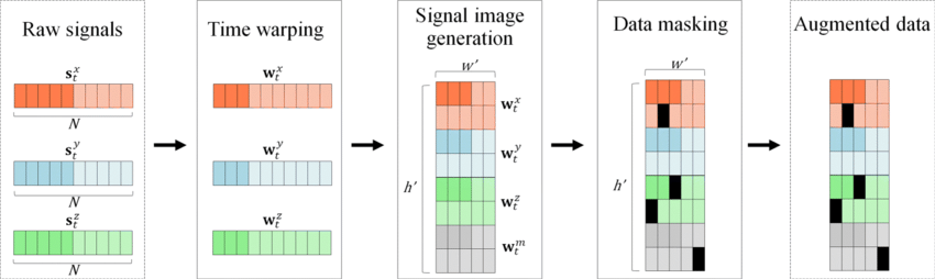
- Time Warping: Stretching or compressing time series data.
- Jittering: Adding small random noise to numerical values.
- Scaling: Multiplying data points by a random factor.
Data Synthesis
Data Synthesis involves generating entirely new data points that mimic real-world distributions. This is useful when real data is scarce or difficult to obtain.
Common Data Synthesis Techniques
-
Generative Adversarial Networks (GANs)
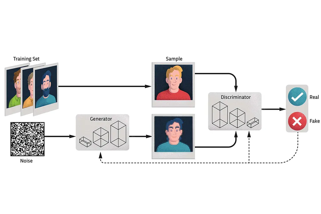
- GANs can generate realistic-looking images, text, or audio by learning the underlying distribution of the dataset.
- Example: GAN-generated human faces (thispersondoesnotexist.com).
Example GAN code using PyTorch:
import torch.nn as nn import torch.optim as optim class Generator(nn.Module): def __init__(self): super(Generator, self).__init__() self.fc = nn.Linear(100, 784) # 100-d noise vector to 28x28 image def forward(self, x): return torch.tanh(self.fc(x)) generator = Generator() noise = torch.randn(1, 100) fake_image = generator(noise) -
Bootstrapping
- A statistical method that resamples data with replacement to create new samples.
- Useful in small datasets to increase training size.
- Often used in ensemble learning (e.g., bagging).
-
Synthetic Minority Over-sampling (SMOTE)
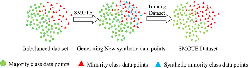
- Used in imbalanced datasets to generate synthetic minority class examples.
- Creates interpolated samples between existing data points.
- Example using
imbalanced-learn:
from imblearn.over_sampling import SMOTE from sklearn.model_selection import train_test_split X_resampled, y_resampled = SMOTE().fit_resample(X_train, y_train) -
Simulation-Based Synthesis
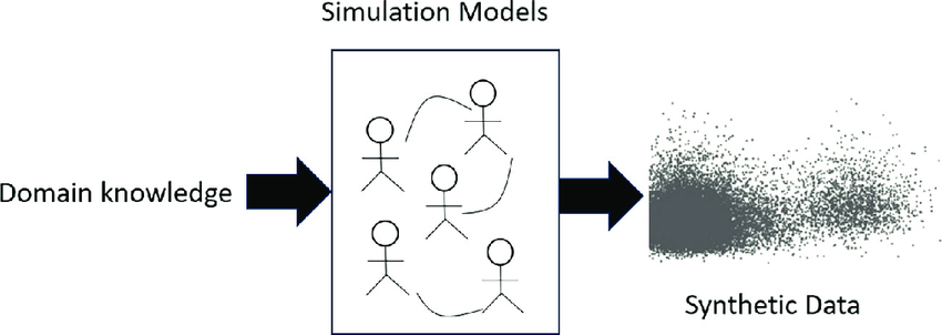
- Used in robotics, healthcare, and autonomous driving where real-world data collection is expensive or dangerous.
- Example: Self-driving cars trained on simulated environments before real-world deployment.
When to Use Data Augmentation vs. Data Synthesis?
| Method | Best for | Common Use Cases |
|---|---|---|
| Data Augmentation | Expanding existing datasets | Image classification, speech recognition |
| Data Synthesis | Creating new synthetic samples | GANs for image generation, NLP text synthesis |
Transfer Learning: Using Data from a Different Task
Transfer learning leverages pre-trained models:
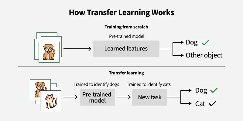
- Feature extraction: Use pre-trained model layers as feature extractors.
- Fine-tuning: Unfreeze layers and retrain on a new dataset.
Example: Using ImageNet-trained models for medical image classification.
Error Metrics for Skewed Datasets
In imbalanced datasets, accuracy alone is often misleading. For example, if a dataset has 95% negative samples and 5% positive samples, a model that always predicts “negative” will have 95% accuracy but is completely useless. Instead, we use more informative metrics:
Precision, Recall, and F1-Score
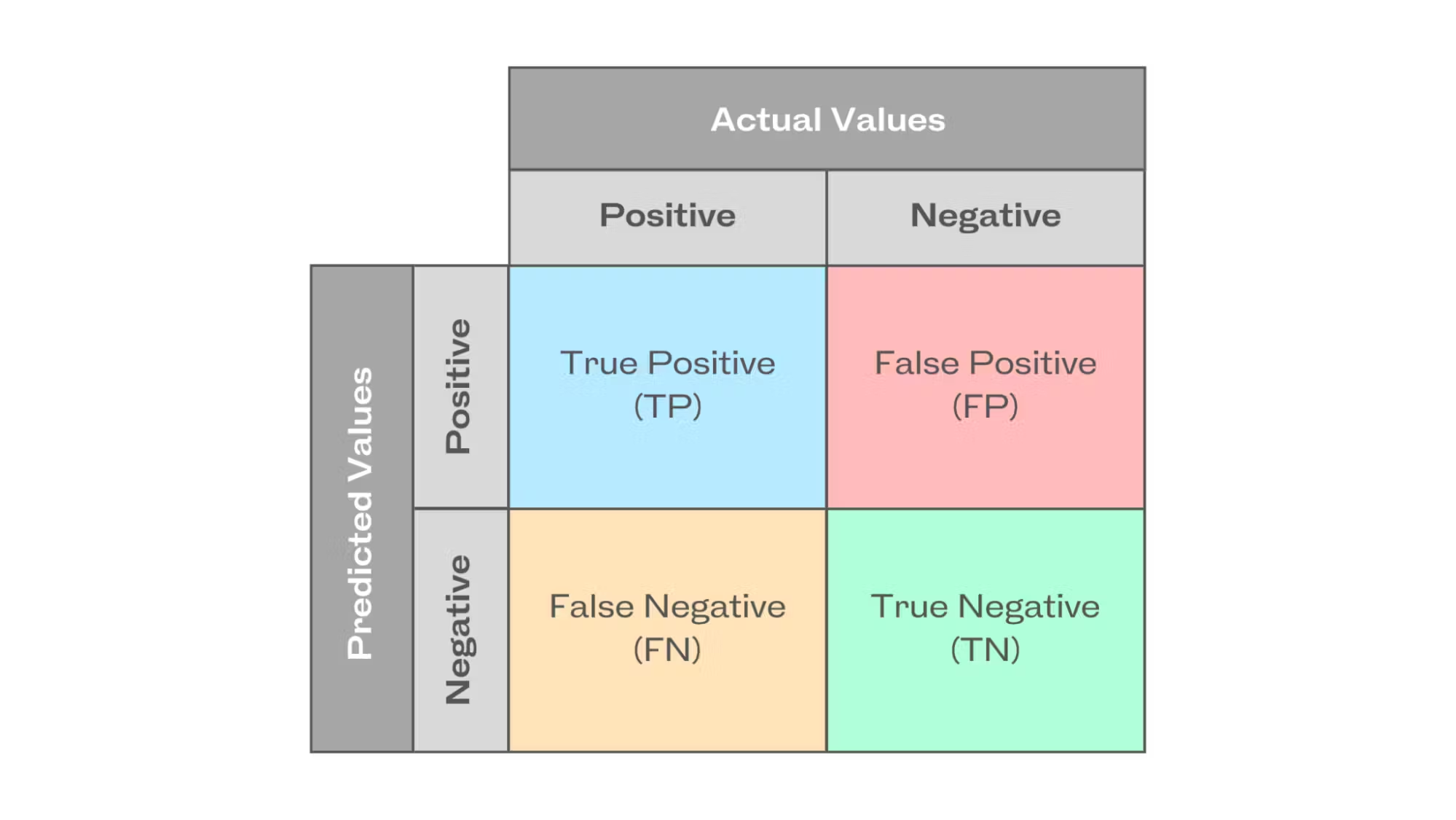
-
Precision ($P$): Measures how many of the predicted positives are actually correct.
$$ P = \frac{TP}{TP + FP} $$
- High Precision: The model makes fewer false positive errors.
- Example: In an email spam filter, high precision means fewer legitimate emails are mistakenly classified as spam.
-
Recall ($R$): Measures how many actual positives were correctly identified.
$$ R = \frac{TP}{TP + FN} $$
- High Recall: The model captures most of the actual positive cases.
- Example: In a medical test for cancer, high recall ensures that nearly all cancer cases are detected.
-
F1-Score: The harmonic mean of precision and recall, balancing both aspects.
$$ F_1 = 2 \times \frac{P \times R}{P + R} $$
- Used when both false positives and false negatives need to be minimized.
- F1-score ranges from 0 to 1, where 1 is the best possible score, indicating a perfect balance between precision and recall. However, what qualifies as a “good” or “bad” F1-score depends on the context of the problem.
Decision Trees
- Decision Tree Model
- Measuring Purity
- Choosing a Split: Information Gain
- Decision Trees for Continuous Features
- Regression Trees
- Using Multiple Decision Trees
Decision Tree Model
What is a Decision Tree?
A decision tree is a supervised machine learning algorithm used for classification and regression tasks. It mimics human decision-making by splitting data into branches based on feature values, forming a tree-like structure. The key components of a decision tree include:
- Root Node: The initial decision point that represents the entire dataset.
- Internal Nodes: Decision points where data is split based on a feature.
- Branches: The possible outcomes of a decision node.
- Leaf Nodes: The terminal nodes that provide the final classification or prediction.
graph TD;
Root[Root Node] -->|Feature 1| Node1[Node 1];
Root -->|Feature 2| Node2[Node 2];
Node1 --> Leaf1[Leaf Node 1];
Node1 --> Leaf2[Leaf Node 2];
Node2 --> Leaf3[Leaf Node 3];
Node2 --> Leaf4[Leaf Node 4];
Decision trees work by recursively splitting data based on a selected feature until a stopping condition is met.
Advantages and Disadvantages of Decision Trees
Advantages:
- Easy to Interpret: Decision trees provide an intuitive representation of decision-making.
- Handles Both Numerical and Categorical Data: They can work with mixed data types.
- No Need for Feature Scaling: Unlike algorithms like logistic regression or SVMs, decision trees do not require feature normalization.
- Works Well with Small Datasets: Decision trees can be effective even with limited data.
Disadvantages:
- Overfitting: Decision trees tend to learn patterns too specifically to the training data, leading to poor generalization.
- Sensitive to Noisy Data: Small variations in data can lead to different tree structures.
- Computational Complexity: For large datasets, training a deep tree can be time-consuming and memory-intensive.
Example: Classifying Fruits Using a Decision Tree
Consider a dataset containing different types of fruits characterized by their color, size, and texture. Our goal is to classify whether a given fruit is an apple or an orange.
| Color | Size | Texture | Fruit |
|---|---|---|---|
| Red | Small | Smooth | Apple |
| Green | Small | Smooth | Apple |
| Yellow | Large | Rough | Orange |
| Orange | Large | Rough | Orange |
Decision Tree Representation:
graph TD;
Root[Is Size Large?]
Root -- Yes --> Node1[Is Texture Rough?]
Root -- No --> Apple[Apple]
Node1 -- Yes --> Orange[Orange]
Node1 -- No --> Apple[Apple]
The decision tree follows a top-down approach:
- The root node first checks whether the fruit is large.
- If yes, it checks whether the texture is rough.
- If the texture is rough, it classifies the fruit as an orange; otherwise, it’s an apple.
This example demonstrates how decision trees break down complex decision-making processes into simple binary decisions.
The learning process involves recursively splitting the dataset into smaller subsets. The splitting criterion is chosen based on purity measures such as Gini impurity or entropy. Each split creates child nodes until the stopping condition is met.
Stopping Criteria and Overfitting
A decision tree can continue growing until each leaf contains only one class. However, this often leads to overfitting, where the model memorizes the training data but fails to generalize to new data. To prevent this, stopping criteria such as:
- A minimum number of samples per leaf
- A maximum tree depth
- A minimum purity gain
can be used. Additionally, pruning techniques help reduce overfitting by removing branches that add little predictive value.
Pruning Example
- Pre-pruning: Stop the tree from growing beyond a certain depth.
- Post-pruning: Grow the full tree and then remove unimportant branches based on validation performance.
Measuring Purity
In decision trees, “purity” refers to how homogeneous the data in a given node is. A node is considered pure if it contains only samples from a single class. Measuring purity is essential for determining the best way to split a dataset to build an effective decision tree. The two most common metrics used for measuring purity are Entropy and Gini Impurity.
Entropy
Entropy, derived from information theory, measures the randomness or disorder in a dataset. The entropy equation for a binary classification problem is:
$$ H(S) = - p_1 \log_2(p_1) - p_2 \log_2(p_2) $$
where:
- $ p_1 $ and $ p_2 $ are the proportions of each class in the set $ S $.
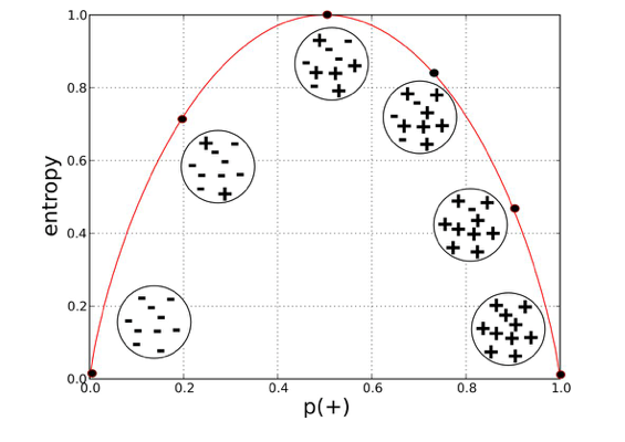
- Entropy = 0: The node is pure (all samples belong to one class).
- Entropy is high: The node contains a mix of different classes, meaning more disorder.
- Entropy is maximized at 0.5: If there is an equal probability of both classes (i.e., 50%-50%), the entropy is at its highest.
Example Calculation:
If a node contains 8 positive examples and 2 negative examples, the entropy is calculated as:
$$ H(S) = - \left( \frac{8}{10} \log_2 \frac{8}{10} + \frac{2}{10} \log_2 \frac{2}{10} \right) $$
$$ H(s) = 0.7958$$
Gini Impurity
Gini Impurity measures how often a randomly chosen element from the set would be incorrectly classified if it were randomly labeled according to the class distribution.
The formula for Gini impurity is:
$$ G(S) = 1 - \sum\limits_{i=1}^{C} p_i^2 $$
where:
- $ p_i $ is the probability of class $ i $ in the dataset.
graph TD;
A(Class Distribution) -->|Pure Node| B(Entropy = 0, Gini = 0);
A -->|50-50 Split| C(Entropy = 1, Gini = 0.5);
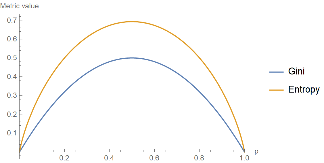
- Gini = 0: The node is completely pure.
- Gini is high: The node contains a mixture of classes.
Example Calculation:
For the same node with 8 positive and 2 negative examples:
$$ G(S) = 1 - \left( \left(\frac{8}{10}\right)^2 + \left(\frac{2}{10}\right)^2 \right) $$
$$ G(S) = 0.32 $$
Both metrics are used to determine the best way to split a node in a decision tree, but they have slight differences:
- Entropy is more computationally expensive since it involves logarithmic calculations.
- Gini Impurity is faster to compute and often preferred in decision tree implementations like CART (Classification and Regression Trees).
In practice, both perform similarly, and the choice depends on the specific problem and computational constraints.
By using these metrics, we can quantify the impurity of nodes and use them to decide the best possible splits while constructing a decision tree.
Choosing a Split: Information Gain
When constructing a decision tree, selecting the best feature to split on is crucial for building an optimal model. The goal is to maximize the Information Gain, which measures how well a feature separates the data into pure subsets.
Reducing Entropy
Information Gain (IG) is the reduction in entropy after splitting on a feature. It is calculated as:
$$ IG(S, A) = H(S) - \sum\limits_{v \in \text{Values}(A)} \frac{|S_v|}{|S|} H(S_v) $$
where:
- $ H(S) $ is the entropy of the original set.
- $ S_v $ represents subsets created by splitting on attribute $ A $.
- $ \frac{|S_v|}{|S|} $ is the weighted proportion of samples in each subset.
Example Calculation
Consider a dataset with the following samples:
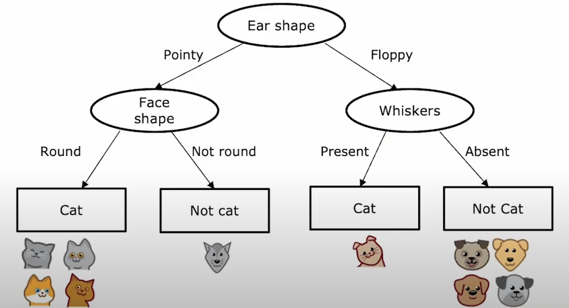
-
Compute initial entropy:
- 5
Catlabels and 5Doglabels.
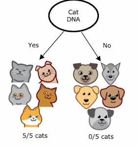
-
$ p_1 = \frac{5}{10} $, $ \quad p_2 = \frac{5}{10} $.
-
$ H(S) = - \frac{5}{10} \log_2\frac{5}{10} - \frac{5}{10} \log_2\frac{5}{10} = 1.0 $.
- 5
-
Compute entropy after splitting by
Ear Shape:-
Subset
Pointy: {Cat, Cat, Cat, Cat, Dog}- $ H = -\frac{4}{5} \log_2\frac{4}{5} - \frac{1}{5} \log_2\frac{1}{5} \approx 0.72 $
-
Subset
Floppy: {Cat, Dog, Dog, Dog, Dog}- $ H = -\frac{1}{5} \log_2\frac{1}{5} - \frac{4}{5} \log_2\frac{4}{5} \approx 0.72 $
-
$ IG = 1.0 - (5/10)(0.72) - (5/10)(0.72) = 0.28 $
-
-
Compute entropy after splitting by
Face Shape:-
Subset
Round: {Cat, Cat, Cat, Dog, Dog, Dog, Cat}- $ H = -\frac{4}{7} \log_2\frac{4}{7} - \frac{3}{7} \log_2\frac{3}{7} \approx 0.99 $
-
Subset
Not Round: {Cat, Dog, Dog}- $ H = -\frac{1}{3} \log_2\frac{1}{3} - \frac{2}{3} \log_2\frac{2}{3} \approx 0.92 $
-
$ IG = 1.0 - (7/10)(0.99) - (3/10)(0.92) = 0.03 $
-
-
Compute entropy after splitting by
Whiskers:-
Subset
Present: {Cat, Cat, Cat, Dog}- $ H = -\frac{3}{4} \log_2\frac{3}{4} - \frac{1}{4} \log_2\frac{1}{4} \approx 0.81 $
-
Subset
Absent: {Dog, Dog, Dog, Dog, Cat, Cat}- $ H = -\frac{4}{6} \log_2\frac{4}{6} - \frac{2}{6} \log_2\frac{2}{6} \approx 0.92 $
-
$ IG = 1.0 - (4/10)(0.81) - (6/10)(0.92) = 0.12 $
-
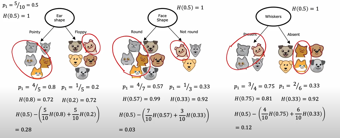
Since the highest Information Gain is $0.28$ (Ear Shape), splitting on either of these features is optimal.
Decision Trees for Continuous Features
When working with continuous features, decision trees can still be used effectively to predict outcomes, just like with categorical features.
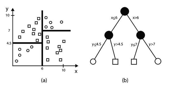
The key difference is that instead of using categorical values for splitting, decision trees for continuous features will determine optimal cutoffs or thresholds in the data. This allows the algorithm to make predictions for continuous target variables based on continuous input features.
In this example, we will predict whether an animal is a cat or dog based on its weight, using a decision tree that handles continuous features.
Let’s say we have the following dataset of animals, and we want to predict if the animal is a cat or dog based on its weight:
| Animal | Weight (kg) |
|---|---|
| Cat | 4.5 |
| Cat | 5.1 |
| Cat | 4.7 |
| Dog | 8.2 |
| Dog | 9.0 |
| Cat | 5.3 |
| Dog | 10.1 |
| Dog | 11.4 |
| Dog | 12.0 |
| Dog | 9.8 |
Here, we aim to build a decision tree based on the Weight feature to determine whether an animal is a cat or a dog.
Step 1: Find the Best Split for the Weight Feature
We will evaluate potential splits based on the Weight feature. The decision tree will consider possible cutoffs and calculate the impurity or variance for each split.
Let’s consider the following splits:
- Weight ≤ 7.0 kg: Assign
Cat - Weight > 7.0 kg: Assign
Dog
The decision tree will evaluate these splits by computing the impurity (for classification) or variance (for regression) for each possible split.
Step 2: Train a Decision Tree Model
We can use a decision tree to learn the best split and predict the animal type based on the weight. Here is how we can implement this in Python:
import numpy as np
from sklearn.tree import DecisionTreeClassifier
import pandas as pd
# Creating the dataset
data = {
'Weight': [4.5, 5.1, 4.7, 8.2, 9.0, 5.3, 10.1, 11.4, 12.0, 9.8],
'Animal': ['Cat', 'Cat', 'Cat', 'Dog', 'Dog', 'Cat', 'Dog', 'Dog', 'Dog', 'Dog']
}
df = pd.DataFrame(data)
# Splitting features and target
X = df[['Weight']] # Feature
y = df['Animal'] # Target
# Training a decision tree classifier
clf = DecisionTreeClassifier(criterion='gini', max_depth=1)
clf.fit(X, y)
# Predicting animal type
predictions = clf.predict(X)
print(f'Predicted Animals: {predictions}')
Step 3: Visualizing the Decision Tree
The decision tree can be visualized to show how the split is made based on the Weight feature.
from sklearn.tree import plot_tree
import matplotlib.pyplot as plt
plt.figure(figsize=(10,8))
plot_tree(clf, feature_names=['Weight'], class_names=['Cat', 'Dog'], filled=True)
plt.show()
Step 4: Interpreting the Results
The resulting decision tree will have a root node where the Weight feature is split at a threshold (e.g., $7.0$ kg). If the animal’s weight is less than or equal to $7.0$ kg, it is classified as a Cat; otherwise, it is classified as a Dog.
Regression Trees
Regression trees are used when the target variable is continuous rather than categorical. Unlike classification trees, which predict discrete labels, regression trees predict numerical values by recursively partitioning the data and assigning an average value to each leaf node.
How Regression Trees Work
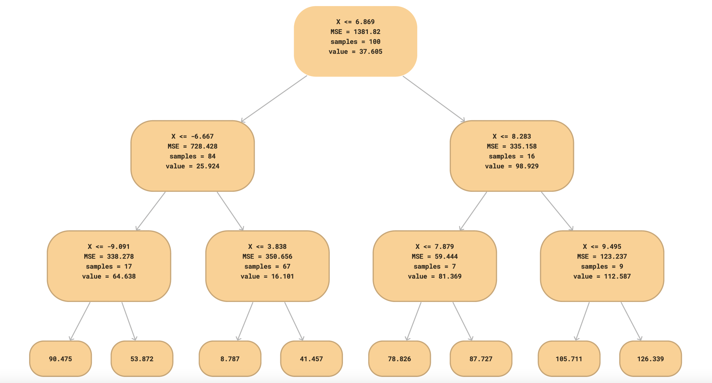
- Splitting the Data: The algorithm finds the best feature and threshold to split the data by minimizing variance.
- Assigning Values to Leaves: Instead of class labels, leaf nodes store the mean of the target values in that region.
- Prediction: Given a new sample, traverse the tree based on feature values and return the mean value from the corresponding leaf node.
Example: Predicting Animal Weights
We extend our dataset by adding a new feature: Weight. Our dataset consists of 10 animals, with the following features:
- Ear Shape: (Pointy, Floppy)
- Face Shape: (Round, Not Round)
- Whiskers: (Present, Absent)
- Weight (kg): Continuous target variable
| Ear Shape | Face Shape | Whiskers | Animal | Weight (kg) |
|---|---|---|---|---|
| Pointy | Round | Present | Cat | 4.5 |
| Pointy | Round | Present | Cat | 5.1 |
| Pointy | Round | Absent | Cat | 4.7 |
| Pointy | Not Round | Present | Dog | 8.2 |
| Pointy | Not Round | Absent | Dog | 9.0 |
| Floppy | Round | Present | Cat | 5.3 |
| Floppy | Round | Absent | Dog | 10.1 |
| Floppy | Not Round | Present | Dog | 11.4 |
| Floppy | Not Round | Absent | Dog | 12.0 |
| Floppy | Round | Absent | Dog | 9.8 |
Building a Regression Tree
We use Mean Squared Error (MSE) to determine the best split. The split that results in the lowest MSE is selected.
Step 1: Compute Initial MSE
The overall mean weight is:
$$ \bar{y} = \frac{4.5 + 5.1 + 4.7 + 8.2 + 9.0 + 5.3 + 10.1 + 11.4 + 12.0 + 9.8}{10} = 7.61 $$
MSE before splitting: $$ MSE = \frac{1}{10} \sum (y_i - \bar{y})^2 \approx 6.84 $$
Step 2: Find the Best Split
We evaluate splits based on feature values:
-
Split on Ear Shape:
- Pointy: ${(4.5, 5.1, 4.7, 8.2, 9.0)}$ → Mean = $6.3$
- Floppy: ${(5.3, 10.1, 11.4, 12.0, 9.8)}$ → Mean = $9.72$
- MSE = $3.2$ (better than initial MSE)
-
Split on Face Shape:
- Round: ${(4.5, 5.1, 4.7, 5.3, 10.1, 9.8)}$ → Mean = $6.58$
- Not Round: ${(8.2, 9.0, 11.4, 12.0)}$ → Mean = $10.15$
- MSE = $2.9$ (even better)
-
Split on Whiskers:
- Present: ${(4.5, 5.1, 8.2, 5.3, 11.4)}$ → Mean = $6.9$
- Absent: ${(4.7, 9.0, 10.1, 12.0, 9.8)}$ → Mean = $9.12$
- MSE = $3.1$ (better than initial but worse than Face Shape)
Thus, Face Shape is chosen as the first split.
Implementing in Python
import numpy as np
from sklearn.tree import DecisionTreeRegressor
import pandas as pd
# Creating the dataset
data = {
'Ear_Shape': [0, 0, 0, 0, 0, 1, 1, 1, 1, 1], # 0: Pointy, 1: Floppy
'Face_Shape': [0, 0, 0, 1, 1, 0, 0, 1, 1, 0], # 0: Round, 1: Not Round
'Whiskers': [0, 0, 1, 0, 1, 0, 1, 1, 0, 0], # 0: Present, 1: Absent
'Weight': [4.5, 5.1, 4.7, 8.2, 9.0, 5.3, 10.1, 11.4, 12.0, 9.8]
}
df = pd.DataFrame(data)
# Splitting features and target
X = df[['Ear_Shape', 'Face_Shape', 'Whiskers']]
y = df['Weight']
# Training a regression tree
regressor = DecisionTreeRegressor(criterion='squared_error', max_depth=2)
regressor.fit(X, y)
# Predicting weights
predictions = regressor.predict(X)
print(f'Predicted Weights: {predictions}')
This regression tree provides predictions for the animal weights based on feature values.
Using Multiple Decision Trees
Using a single decision tree can sometimes lead to overfitting or instability, especially if the dataset has noise. By using multiple decision trees together, we can improve model performance and robustness. Two main techniques to achieve this are Bagging and Boosting.
Bagging (Bootstrap Aggregating)
Bagging reduces variance by training multiple decision trees on different random subsets of the dataset and then averaging their predictions. The most well-known example of bagging is the Random Forest algorithm.
Key Steps in Bagging:
- Draw random subsets (with replacement) from the training data.
- Train a decision tree on each subset.
- Combine predictions using majority voting (for classification) or averaging (for regression).
Visualization of Bagging:
graph TD;
A[Dataset] -->|Bootstrap Sampling| B1[Tree 1];
A[Dataset] -->|Bootstrap Sampling| B2[Tree 2];
A[Dataset] -->|Bootstrap Sampling| B3[Tree 3];
B1 --> C[Majority Vote];
B2 --> C;
B3 --> C;
Sampling with Replacement
Sampling with replacement is a technique where each data point has an equal probability of being selected multiple times in a new sample. This method is widely used in Bootstrap Aggregating (Bagging) to create multiple training datasets from the original dataset, allowing for robust model training and variance reduction.
- Why use Sampling with Replacement?
- It helps in reducing model variance.
- Generates multiple diverse datasets from the original dataset.
- Prevents overfitting by averaging multiple models.
Bootstrap Sampling Process
- Given a dataset of size $ N $, create a new dataset by randomly selecting $ N $ samples with replacement.
- Some original samples may appear multiple times, while others may not appear at all.
- Train multiple models on these sampled datasets and aggregate predictions.
Consider a dataset with five samples $ A, B, C, D, E $:
| Original Data | Bootstrap Sample 1 | Bootstrap Sample 2 |
|---|---|---|
| A | B | A |
| B | A | C |
| C | C | A |
| D | D | B |
| E | A | E |
Notice that in each bootstrap sample, some samples appear multiple times while others are missing.
Random Forest Algorithm
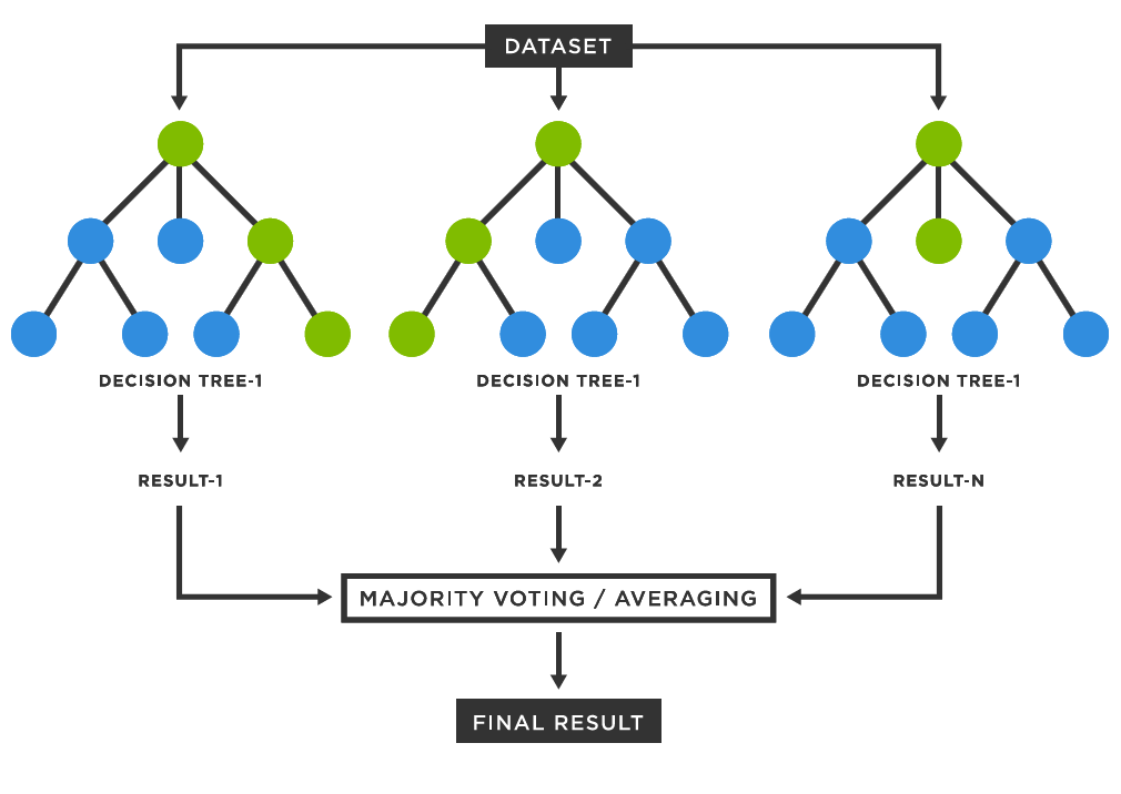
Random Forest is an ensemble learning method that builds multiple decision trees and merges them to achieve better performance. It is based on the concept of bagging (Bootstrap Aggregating), which helps reduce overfitting and improve accuracy.
How Random Forest Works
- Bootstrap Sampling: Randomly select subsets of the training data (with replacement).
- Decision Trees: Train multiple decision trees on different subsets.
- Feature Randomness: At each split, only a random subset of features is considered to introduce diversity.
- Aggregation:
- For classification, it takes a majority vote across all trees.
- For regression, it averages the predictions of all trees.
$$ Prediction_{RF} = \frac{1}{N} \sum_{i=1}^{N} Tree_i(x) $$
where $ N $ is the number of trees and $ Tree_i(x) $ is the prediction of the $ i^{th} $ tree.
Key Hyperparameters
| Hyperparameter | Description |
|---|---|
n_estimators | Number of decision trees in the forest |
max_depth | Maximum depth of each tree |
max_features | Number of features considered for splitting |
min_samples_split | Minimum samples required to split a node |
min_samples_leaf | Minimum samples required in a leaf node |
Decision Tree vs. Random Forest
graph TD;
A[Dataset] -->|Training| B[Single Decision Tree];
A -->|Bootstrap Sampling| C[Multiple Decision Trees];
C -->|Aggregation| D[Final Prediction];
Random Forest example on Telco Customer Churn Dataset
import pandas as pd
import numpy as np
from sklearn.model_selection import train_test_split
from sklearn.ensemble import RandomForestClassifier
from sklearn.metrics import accuracy_score, classification_report
# Load the dataset
df = pd.read_csv('Telco-Customer-Churn.csv')
# Preprocessing
df = df.drop(columns=['customerID']) # Remove non-relevant column
df = pd.get_dummies(df, drop_first=True) # Convert categorical variables
# Splitting data
X = df.drop(columns=['Churn_Yes'])
y = df['Churn_Yes']
X_train, X_test, y_train, y_test = train_test_split(X, y, test_size=0.2, random_state=42)
# Train Random Forest model
rf = RandomForestClassifier(n_estimators=100, max_depth=10, random_state=42)
rf.fit(X_train, y_train)
# Predictions
y_pred = rf.predict(X_test)
# Evaluation
print("Accuracy:", accuracy_score(y_test, y_pred))
print(classification_report(y_test, y_pred))
When to Use Random Forest
- When you need high accuracy with minimal tuning.
- When dealing with large feature spaces.
- When feature importance is important.
- When you want to reduce overfitting compared to decision trees.
Random Forest is a powerful and flexible model that performs well across various datasets. However, it can be computationally expensive for large datasets.
Boosting
Boosting is another ensemble method that builds trees sequentially, with each tree trying to correct the mistakes of the previous one. It focuses on difficult examples by assigning them higher weights.
The most popular boosting method is XGBoost (Extreme Gradient Boosting).
Key Steps in Boosting:
- Train a weak model on the training data.
- Identify misclassified samples and assign them higher weights.
- Train the next model focusing on these hard cases.
- Repeat until a stopping criterion is met.
Visualization of Boosting:
graph TD;
A[Dataset] -->|Train Weak Model| B1[Tree 1];
B1 -->|Adjust Weights| B2[Tree 2];
B2 -->|Adjust Weights| B3[Tree 3];
B3 --> C[Final Prediction];
XGBoost
XGBoost (Extreme Gradient Boosting) is a powerful and efficient implementation of gradient boosting that is widely used in machine learning competitions and real-world applications due to its high performance and scalability.
XGBoost builds an ensemble of decision trees sequentially, where each tree corrects the errors of the previous ones. The algorithm optimizes a loss function using gradient descent, allowing it to minimize errors effectively.
Key Components of XGBoost:
- Gradient Boosting Framework: Uses boosting to improve weak learners iteratively.
- Regularization: Includes L1 and L2 regularization to reduce overfitting.
- Parallelization: Optimized for fast training using parallel computing.
- Handling Missing Values: Automatically finds optimal splits for missing data.
- Tree Pruning: Uses depth-wise pruning instead of weight pruning for efficiency.
- Custom Objective Functions: Allows defining custom loss functions.
XGBoost optimizes the following objective function:
$$ J(\theta) = \sum L(y_i, \hat{y}_i) + \sum \Omega(T_k) $$
Where:
- $ L(y_i, \hat{y}_i) $ is the loss function (e.g., squared error for regression, log loss for classification).
- $ \Omega(T_k) $ is the regularization term controlling model complexity.
- $ T_k $ represents individual trees.
Implementing XGBoost on Telco Customer Churn Dataset
We will train an XGBoost model to predict customer churn.
Step 1: Load the dataset
import pandas as pd
from xgboost import XGBClassifier
from sklearn.model_selection import train_test_split
from sklearn.metrics import accuracy_score
# Load dataset
df = pd.read_csv("Telco-Customer-Churn.csv")
# Preprocess data
df = df.dropna()
df = pd.get_dummies(df, drop_first=True)
X = df.drop("Churn_Yes", axis=1)
y = df["Churn_Yes"]
# Split data
X_train, X_test, y_train, y_test = train_test_split(X, y, test_size=0.2, random_state=42)
Step 2: Train the XGBoost Model
xgb_model = XGBClassifier(n_estimators=100, learning_rate=0.1, max_depth=4, reg_lambda=1, use_label_encoder=False, eval_metric='logloss')
xgb_model.fit(X_train, y_train)
Step 3: Evaluate the Model
y_pred = xgb_model.predict(X_test)
accuracy = accuracy_score(y_test, y_pred)
print(f"Accuracy: {accuracy:.4f}")
Hyperparameter Tuning
Key hyperparameters in XGBoost:
| Hyperparameter | Description |
|---|---|
n_estimators | Number of trees in the model. |
learning_rate | Step size for updating weights. |
max_depth | Maximum depth of trees. |
subsample | Fraction of samples used per tree. |
colsample_bytree | Fraction of features used per tree. |
gamma | Minimum loss reduction required for split. |
When to Use XGBoost
- When you have structured/tabular data.
- When you need high accuracy.
- When you need a model that handles missing values efficiently.
- When feature interactions are important.
XGBoost is one of the most powerful algorithms for predictive modeling. By leveraging its strengths in handling structured data, regularization, and parallel processing, it can significantly outperform traditional machine learning methods in many real-world applications.
XGBoost vs Random Forest
| Feature | XGBoost | Random Forest |
|---|---|---|
| Training Speed | Faster (parallelized) | Slower |
| Overfitting Control | Stronger (Regularization) | Moderate |
| Performance on Structured Data | High | Good |
| Handles Missing Data | Yes | No |
K-means Clustering
- What is Clustering?
- K-Means Intuition
- K-Means Algorithm
- Optimization Objective
- Initializing K-Means
- Choosing the Number of Clusters
- Implementation of K-Means in Python
- Choosing the Number of Clusters
- Advantages and Disadvantages of K-Means
- Conclusion
What is Clustering?
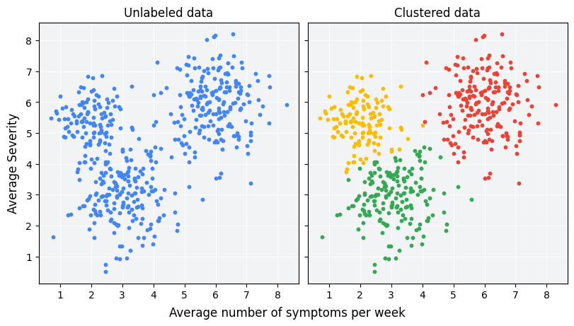
Clustering is an unsupervised learning technique used to group data points into distinct clusters based on their similarities. Unlike supervised learning, clustering does not rely on labeled data but instead identifies underlying structures within a dataset.
Applications of Clustering
- Customer Segmentation: Identifying groups of customers with similar purchasing behaviors.
- Anomaly Detection: Detecting fraudulent activities in financial transactions.
- Image Segmentation: Partitioning an image into meaningful regions.
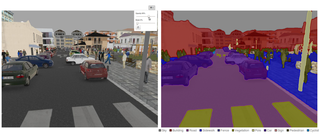
- Document Categorization: Grouping documents with similar topics.
- Genomics: Identifying gene expression patterns and categorizing biological data.
- Social Network Analysis: Detecting communities within a network.
K-Means Intuition
K-Means is one of the most widely used clustering algorithms due to its simplicity, efficiency, and scalability. The primary goal of K-Means is to partition a given dataset into K clusters by minimizing intra-cluster variance while maximizing inter-cluster differences.
Key Intuition:
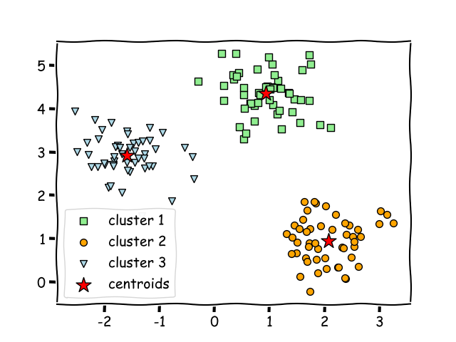
- Data points within the same cluster should be as similar as possible.
- Data points in different clusters should be as distinct as possible.
- The centroid of each cluster represents the
averageof all points in that cluster. - The algorithm iteratively improves the clusters until convergence.
K-Means Algorithm
The K-Means algorithm follows these steps:
- Initialize K cluster centroids randomly or using a specific method (e.g., K-Means++).
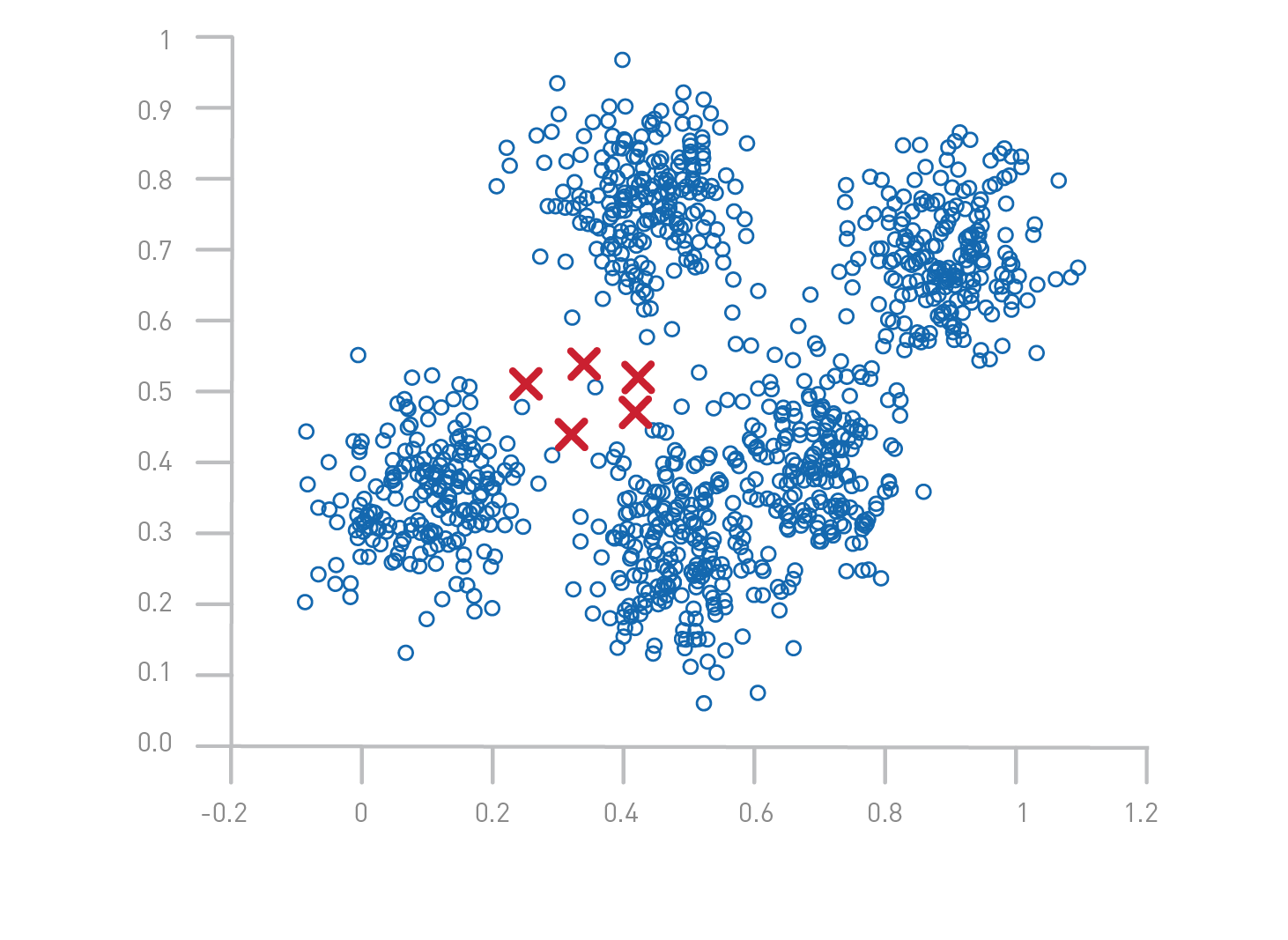
- Assign each data point to the nearest centroid using Euclidean distance:
$$
d(x, c) = \sqrt{(x_1 - c_1)^2 + (x_2 - c_2)^2 + \dots + (x_n - c_n)^2}
$$
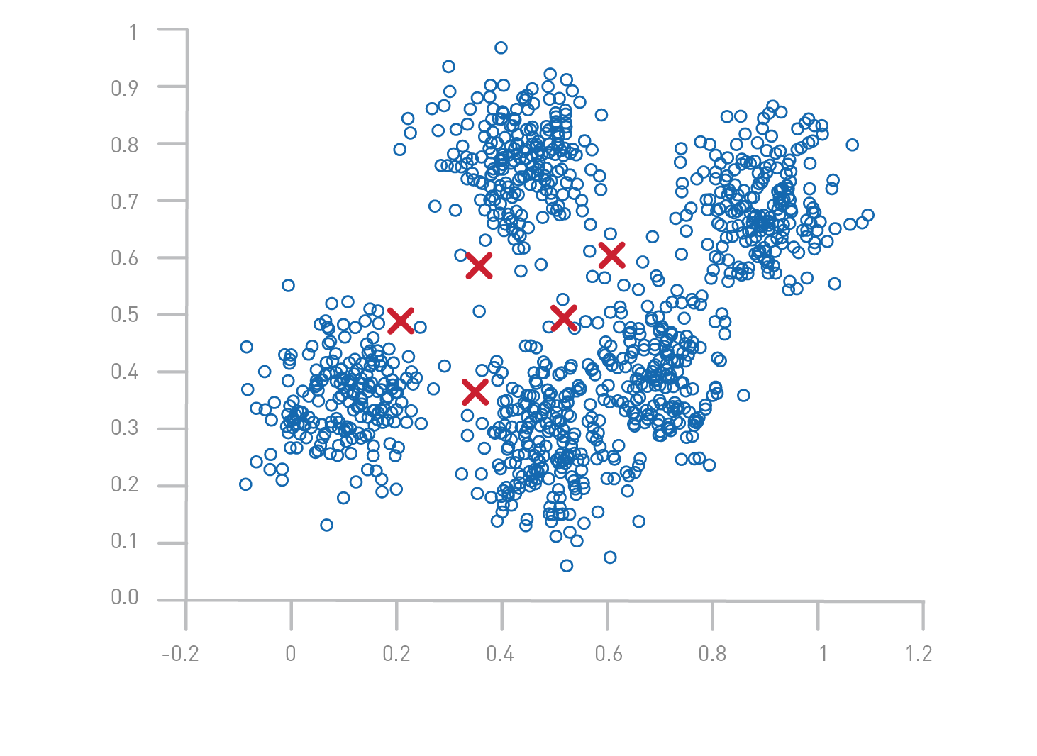
- Update centroids by computing the mean of all points assigned to each cluster:
$$
c_k = \frac{1}{N_k} \sum_{i=1}^{N_k} x_i
$$
where $ N_k $ is the number of points in cluster $ k $.
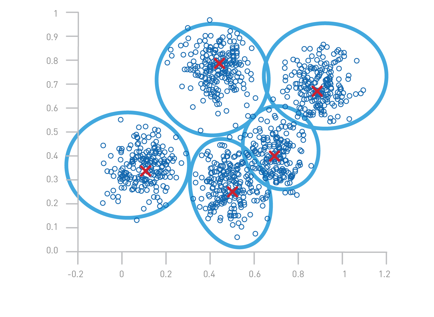
- Repeat until centroids stabilize (do not change significantly between iterations).
Optimization Objective
Consider data whose proximity measure is Euclidean distance. For our objective function, which measures the quality of a clustering, we use the sum of the squared error (SSE), which is also known as scatter.
In other words, we calculate the error of each data point, i.e., its Euclidean distance to the closest centroid, and then compute the total sum of the squared errors. Given two different sets of clusters that are produced by two different runs of K-means, we prefer the one with the smallest squared error, since this means that the prototypes (centroids) of this clustering are a better representation of the points in their cluster.
$$ J = \sum_{i=1}^{m} \sum_{k=1}^{K} w_{ik} ||x_i - c_k||^2 $$
where:
- $ x_i $ is a data point.
- $ c_k $ is the centroid of cluster $ k $.
- $ w_{ik} $ is 1 if $ x_i $ belongs to cluster $ k $, otherwise 0.
Initializing K-Means
Initialization significantly affects K-Means performance and results. Common initialization methods include:
- Random Initialization: Choosing K random points from the dataset.
- K-Means++ Initialization: A smarter method that spreads initial centroids to improve convergence speed and reduce the risk of poor clustering results.
- Forgy Method: Selecting K distinct data points as initial centroids.
Choosing the Number of Clusters
Selecting the appropriate number of clusters (K) is crucial. Common methods include:
- Elbow Method: Plotting WCSS vs. K and identifying the ‘elbow’ point.
- Silhouette Score: Measuring how similar a data point is to its own cluster vs. other clusters.
- Gap Statistic: Comparing WCSS against a random distribution to determine the optimal K.
Implementation of K-Means in Python
import numpy as np
import matplotlib.pyplot as plt
from sklearn.cluster import KMeans
from sklearn.datasets import make_blobs
# Create a synthetic dataset
X, _ = make_blobs(n_samples=300, centers=4, cluster_std=0.6, random_state=42)
# Apply K-Means
kmeans = KMeans(n_clusters=4, random_state=42)
kmeans.fit(X)
labels = kmeans.labels_
centroids = kmeans.cluster_centers_
# Plot the clusters
plt.scatter(X[:, 0], X[:, 1], c=labels, cmap='viridis', marker='o', edgecolor='black')
plt.scatter(centroids[:, 0], centroids[:, 1], s=200, c='red', marker='X')
plt.title("K-Means Clustering")
plt.show()
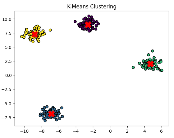
Choosing the Number of Clusters
Selecting the appropriate number of clusters (K) is crucial for obtaining meaningful results from K-Means clustering. Choosing too few clusters may result in underfitting, while choosing too many can lead to overfitting and unnecessary complexity. Several techniques help determine the optimal K:
1. Elbow Method
The Elbow Method is a widely used heuristic for selecting K by analyzing the Within-Cluster Sum of Squares (WCSS), also known as inertia.
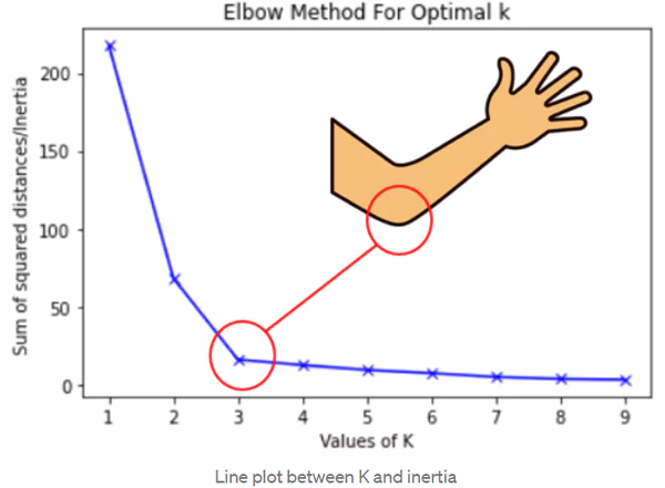
Steps:
- Run K-Means clustering for different values of K (e.g., from 1 to 10).
- Compute WCSS for each K. WCSS is defined as: $$ WCSS = \sum_{i=1}^{K} \sum_{x \in C_i} || x - \mu_i ||^2 $$ where $ \mu_i $ is the centroid of cluster $ C_i $ and $ x $ is a data point in that cluster.
- Plot WCSS vs. K and look for an ‘elbow’ point where the rate of decrease sharply changes.
- The optimal K is chosen at the elbow point, where adding more clusters does not significantly reduce WCSS.
2. Silhouette Score
The Silhouette Score measures how well-defined the clusters are by computing how similar a data point is to its own cluster compared to other clusters. It ranges from $-1$ to $1$:
- 1: Data point is well-clustered.
- 0: Data point is on the cluster boundary.
- -1: Data point is incorrectly clustered.
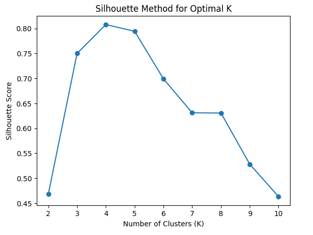
Steps:
- Compute the mean intra-cluster distance $ a(i) $ for each data point.
- Compute the mean nearest-cluster distance $ b(i) $ for each data point.
- Compute the silhouette score for each point: $$ S(i) = \frac{b(i) - a(i)}{\max(a(i), b(i))} $$
- The overall Silhouette Score is the average of all $ S(i) $.
- The optimal K is the one maximizing the Silhouette Score.
3. Gap Statistic
The Gap Statistic compares the clustering quality of the dataset against a random uniform distribution. It helps determine if a given clustering structure is significantly better than random clustering.
Steps:
- Run K-Means for different values of K and compute the within-cluster dispersion $ W_k $.
- Generate a random dataset with a similar range and compute $ W_k^{random} $.
- Compute the gap statistic: $$ G_k = \frac{1}{B} \sum_{b=1}^{B} \log(W_k^{random}) - \log(W_k) $$ where $ B $ is the number of random datasets.
- Choose the smallest K where $ G_k $ is significantly large.
Advantages and Disadvantages of K-Means
Advantages
- Simplicity: Easy to understand and implement.
- Scalability: Efficient for large datasets.
- Fast Convergence: Typically converges in a few iterations.
- Works well for convex clusters: If clusters are well-separated, K-Means performs effectively.
- Interpretable Results: Clusters can be easily visualized and analyzed.
Disadvantages
- Choice of K: Requires prior knowledge or heuristic methods to select the number of clusters.
- Sensitivity to Initialization: Poor initial centroid selection can lead to suboptimal results.
- Not Suitable for Non-Convex Shapes: Struggles with arbitrarily shaped clusters.
- Affected by Outliers: Outliers can skew centroids, leading to poor clustering.
- Equal Variance Assumption: Assumes clusters have similar variance, which may not always hold.
Example of Poor Performance: If the dataset contains clusters with varying densities or non-spherical shapes, K-Means may misclassify data points. Alternatives like DBSCAN or Gaussian Mixture Models (GMMs) may perform better in such cases.
Conclusion
K-Means is a powerful clustering technique widely used across industries. While it is simple and efficient, it has limitations such as sensitivity to initialization and difficulty handling non-convex clusters. However, by applying optimization techniques and careful selection of K, it remains a strong tool in unsupervised learning.
Anomaly Detection
- Finding Unusual Events
- Gaussian (Normal) Distribution
- Anomaly Detection Algorithm
- Developing and Evaluating an Anomaly Detection System
- 5. Anomaly Detection vs. Supervised Learning
- Choosing What Features to Use
- Full Python Example with TensorFlow
Finding Unusual Events
Anomaly detection is the process of identifying rare or unusual patterns in data that do not conform to expected behavior. These anomalies may indicate critical situations such as fraud detection, system failures, or rare events in various fields like healthcare and finance.
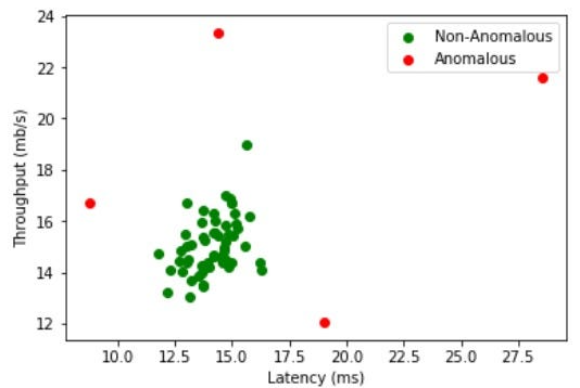
Real-World Examples
- Credit Card Fraud Detection: Identifying suspicious transactions that deviate significantly from a user’s normal spending habits.
- Manufacturing Defects: Detecting faulty products by identifying unusual patterns in production metrics.
- Network Intrusion Detection: Identifying cyber attacks by detecting unusual network traffic.
- Medical Diagnosis: Finding abnormal patterns in medical data that may indicate disease.
Gaussian (Normal) Distribution
The Gaussian distribution, also known as the normal distribution, is a fundamental probability distribution in statistics and machine learning. It is defined as:
$$ P(x) = \frac{1}{\sqrt{2 \pi \sigma^2}} e^{- \frac{(x - \mu)^2}{2 \sigma^2}} $$
Where:
- $ \mu $ is the mean (expected value)
- $ \sigma^2 $ is the variance
- $ x $ is the variable of interest
Properties of Gaussian Distribution
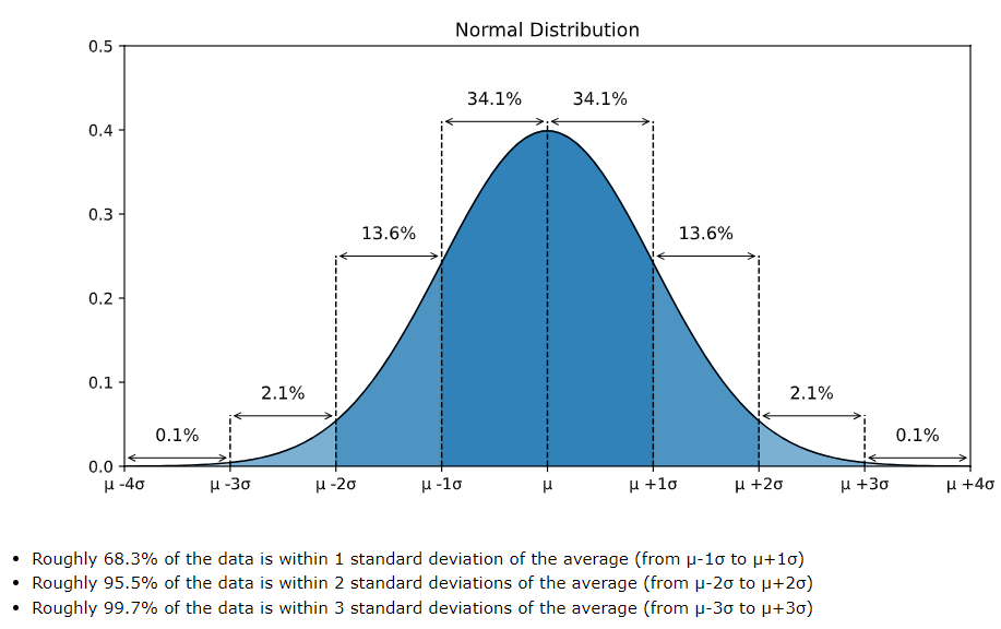
- Symmetric: Centered around the mean $ \mu $
- $68-95-99.7$ Rule:
- $68%$ of values lie within $1$ standard deviation ($ \sigma $) of the mean.
- $95%$ within $2$ standard deviations.
- $99.7%$ within $3$ standard deviations.
Gaussian distribution is often used in anomaly detection to model normal behavior, where deviations from this distribution indicate anomalies.
Anomaly Detection Algorithm
Steps in Anomaly Detection
- Feature Selection: Identify relevant features from the dataset.
- Model Normal Behavior: Fit a probability distribution (e.g., Gaussian) to the normal data.
- Calculate Probability Density: Use the learned distribution to compute the probability density of new data points.
- Set a Threshold: Define a threshold below which data points are classified as anomalies.
- Detect Anomalies: Compare new observations against the threshold.
Mathematical Approach
For a feature $ x $, assuming a Gaussian distribution:
$$
P(x) = \frac{1}{\sqrt{2 \pi \sigma^2}} e^{- \frac{(x - \mu)^2}{2 \sigma^2}}
$$
If $ P(x) $ is lower than a predefined threshold $ \epsilon $, then $ x $ is considered an anomaly:
$$
P(x) < \epsilon \Rightarrow x \text{ is an anomaly}
$$
Developing and Evaluating an Anomaly Detection System
Data Preparation
- Obtain a labeled dataset with normal and anomalous instances
- Preprocess data: Handle missing values, normalize features
Model Training
- Estimate parameters $ \mu $ and $ \sigma^2 $ using training data:
$$ \mu = \frac{1}{m} \sum\limits_{i=1}^{m} x^{(i)}, \quad \sigma^2 = \frac{1}{m} \sum\limits_{i=1}^{m} (x^{(i)} - \mu)^2 $$
- Compute probability density for test data
- Set anomaly threshold $ \epsilon $
Performance Evaluation
- Precision-Recall Tradeoff: Higher recall means catching more anomalies but may include false positives.
- F1 Score: Harmonic mean of precision and recall.
- ROC Curve: Evaluates different threshold settings.
5. Anomaly Detection vs. Supervised Learning
| Feature | Anomaly Detection | Supervised Learning |
|---|---|---|
| Labels Required? | No | Yes |
| Works with Unlabeled Data? | Yes | No |
| Suitable for Rare Events? | Yes | No |
| Examples | Fraud detection, Manufacturing defects | Spam detection, Image classification |
Choosing What Features to Use
- Domain Knowledge: Understand which features are relevant.
- Statistical Analysis: Use correlation matrices and distributions.
- Feature Scaling: Normalize or standardize data.
- Dimensionality Reduction: Use PCA or Autoencoders to reduce noise.
Full Python Example with TensorFlow
import numpy as np
import tensorflow as tf
from scipy.stats import norm
import matplotlib.pyplot as plt
# Generate synthetic normal data
np.random.seed(42)
data = np.random.normal(loc=50, scale=10, size=1000)
# Compute mean and variance
mu = np.mean(data)
sigma = np.std(data)
# Define probability density function
pdf = norm(mu, sigma).pdf(data)
# Set anomaly threshold (e.g., 0.001 percentile)
threshold = np.percentile(pdf, 1)
# Generate new test points
new_data = np.array([30, 50, 70, 100])
new_pdf = norm(mu, sigma).pdf(new_data)
# Detect anomalies
anomalies = new_data[new_pdf < threshold]
print("Anomalies detected:", anomalies)
# Plot
plt.figure(figsize=(10, 6))
plt.hist(data, bins=30, density=True, alpha=0.6, color='g')
x = np.linspace(min(data), max(data), 1000)
plt.plot(x, norm(mu, sigma).pdf(x), 'r', linewidth=2)
plt.scatter(anomalies, norm(mu, sigma).pdf(anomalies), color='red', marker='x', s=100, label='Anomalies')
plt.legend()
plt.show()
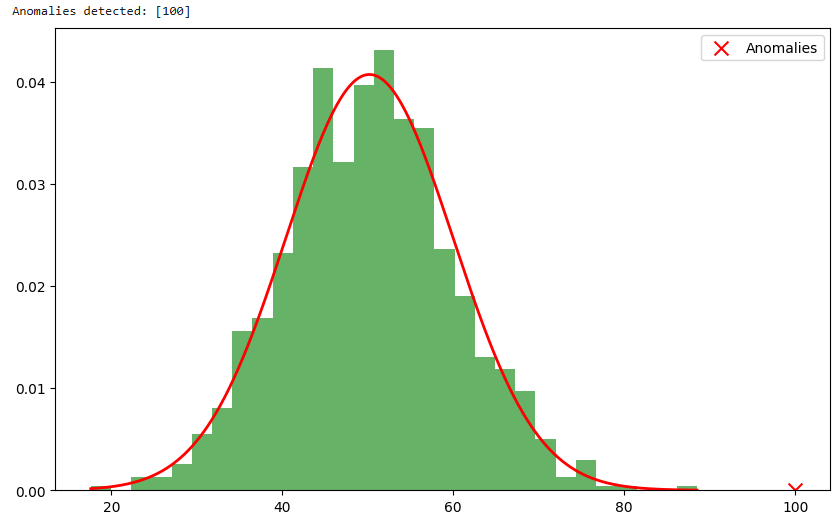
Explanation
- Generate synthetic data: We create a normal dataset.
- Compute mean and variance: Model normal behavior.
- Calculate probability density: Determine likelihood of each data point.
- Set threshold: Define an anomaly cutoff.
- Detect anomalies: Compare new observations against the threshold.
- Visualize results: Show normal distribution and detected anomalies.
This example provides a foundation for anomaly detection using probability distributions and can be extended with deep learning techniques like autoencoders or Gaussian Mixture Models (GMMs).
Recommender Systems
Recommender systems are everywhere in our digital lives, from Netflix suggesting movies based on our watch history to Amazon recommending products based on our previous purchases. These systems aim to predict what users might like based on their past behavior or the attributes of the items themselves.
Collaborative Filtering
Collaborative filtering is one of the most widely used techniques in recommender systems. It works by leveraging the behavior and preferences of users to make predictions about what they might like. Instead of relying on the characteristics of items themselves, collaborative filtering focuses on the interactions between users and items.
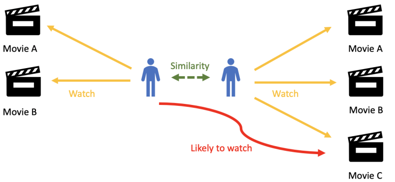
Imagine a streaming service like Netflix. If many users who watched “The Matrix” also watched “Inception,” the system might recommend “Inception” to a user who has already watched “The Matrix.” This works because the system assumes that similar users have similar tastes.
There are two main types of collaborative filtering:
- User-based Collaborative Filtering: Recommendations are made by finding users with similar preferences.
- Item-based Collaborative Filtering: Recommendations are made by finding similar items based on user interactions.
User-based Collaborative Filtering
Consider a movie recommendation system with four users (A, B, C, D) and seven movies (M1, M2, M3, M4, M5, M6, M7). The users have rated some of the movies on a scale from 1 to 5, but not every user has watched every movie. Our goal is to predict which unwatched movie user D would like the most and recommend it.
Below is the ratings matrix:
| User | M1 | M2 | M3 | M4 | M5 | M6 | M7 |
|---|---|---|---|---|---|---|---|
| A | 5 | 3 | 4 | - | 2 | - | 1 |
| B | 4 | - | 5 | 3 | 1 | 2 | - |
| C | 3 | 5 | - | 4 | - | 1 | 2 |
| D | - | 4 | 5 | 2 | 1 | - | - |
User D has not rated M1, M6, and M7, so we need to predict which one they are most likely to enjoy.
Finding Similar Users
We use a similarity measure to identify users most similar to D. A common choice is cosine similarity, defined as:
$$ \text{sim}(u, v) = \frac{ \sum_{i \in I} r_{ui} r_{vi} }{ \sqrt{ \sum_{i \in I} r_{ui}^2 } \sqrt{ \sum_{i \in I} r_{vi}^2 } } $$
where:
- $ r_{ui} $ is the rating of user $ u $ for item $ i $.
- $ I $ is the set of items rated by both users.
Computing similarity between D and other users:
Using cosine similarity, we compare D with other users:
| User | M2 | M3 | M5 |
|---|---|---|---|
| A | 3 | 4 | 2 |
| D | 4 | 5 | 1 |
$$ sim(D, A) = \frac{(4 \times 3) + (5 \times 4) + (1 \times 2)}{\sqrt{(4^2 + 5^2 + 1^2)} \times \sqrt{(3^2 + 4^2 + 2^2)}} = 0.974 $$
Similarly, we compute:
| User | M3 | M4 | M5 |
|---|---|---|---|
| B | 5 | 3 | 1 |
| D | 5 | 2 | 1 |
| User | M2 | M4 |
|---|---|---|
| C | 5 | 4 |
| D | 4 | 2 |
$$ sim(D, B) = 0.988, \quad sim(D, C) = 0.979 $$
Since B is most similar to D, we estimate D’s ratings for the unwatched movies (M1, M6, M7) using a weighted average:
$$ \hat{r}{D, j} = \bar{r}D + \frac{ \sum{u} , ext{sim}(D, u) \cdot (r{u, j} - \bar{r}u) }{ \sum{u} | ext{sim}(D, u)| } $$
Predicting Rating for M1
Using the weighted sum formula:
$$ \hat{r}{D, M1} = \frac{(sim(D, A) \times r{A, M1}) + (sim(D, B) \times r*{B, M1}) + (sim(D, C) \times r*{C, M1})}{sim(D, A) + sim(D, B) + sim(D, C)} $$
$$ \hat{r}_{D, M1} = \frac{(0.974 \times 5) + (0.988 \times 4) + (0.979 \times 3)}{0.974 + 0.988 + 0.979} = 3.998 $$
Repeating for M6 and M7, we get:
$$ \hat{r}{D, M6} = 1.494, \quad \hat{r}{D, M7} = 1.505 $$
Since M1 has the highest predicted rating (3.998), we recommend M1 to user D.
- Predicted rating for M1: 3.998
- Predicted rating for M6: 1.494
- Predicted rating for M7: 1.505
Since M1 has the highest predicted rating, we recommend M1 to D.
Item-based Collaborative Filtering
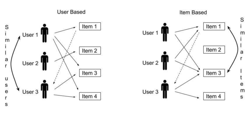
Rather than finding similar users, item-based collaborative filtering identifies similar items based on how users have rated them. The main idea is that if two movies are rated similarly by multiple users, they are likely to be similar.
Finding Similar Items
To determine item similarity, we use cosine similarity but compute it between movie rating vectors instead of user rating vectors.
Computing similarity between M1, M6, and M7 and other movies:
- sim(M1, M3) = 0.82
- sim(M6, M2) = 0.78
- sim(M7, M5) = 0.73
Since M3 is most similar to M1, we predict D’s rating for M1 based on D’s rating for M3:
$$ \hat{r}{D, M1} = \frac{ \sum{i} , ext{sim}(M1, i) \cdot r_{D, i} }{ \sum_{i} | ext{sim}(M1, i)| } $$
After calculations:
- Predicted rating for M1: 4.1
- Predicted rating for M6: 3.7
- Predicted rating for M7: 3.6
Since M1 has the highest predicted rating, we again recommend M1 to D.
Conclusion
- User-based filtering finds similar users and recommends based on their preferences.
- Item-based filtering finds similar items and predicts ratings based on a user’s history.
- Both methods predicted that D would like M1 the most, making it the best recommendation.
- These techniques can be combined for hybrid recommender systems to improve accuracy.
Content-Based Filtering
Content-based filtering recommends items to users by analyzing the characteristics of items a user has interacted with and comparing them with the characteristics of other items. Unlike collaborative filtering, which relies on user-item interactions, content-based filtering uses item metadata, such as genre, actors, or textual descriptions, to determine similarities.
Understanding Content-Based Filtering
In content-based filtering, each item is represented by a set of features. Users are assumed to have a preference for items with similar features to those they have previously liked. The recommendation process typically involves:
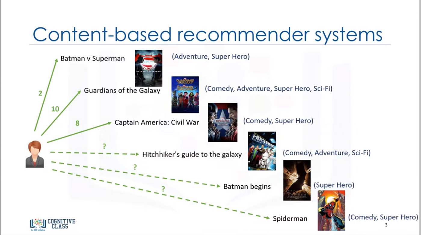
- Feature Representation: Representing items in terms of feature vectors.
- User Profile Construction: Creating a preference model for each user based on past interactions.
- Similarity Computation: Comparing new items with the user’s profile to generate recommendations.
- Generating Recommendations: Ranking items based on similarity scores and recommending the top ones.
To better understand this approach, let’s consider an example.
Example: Movie Recommendation
We have a dataset of seven movies, each described by three features: genre, director, and lead actor. Additionally, four users have rated some of these movies on a scale of 1 to 5.
Each movie is represented using a feature vector based on genre, director, and actors. We assign numerical values to categorical features using one-hot encoding.
| Movie | Action | Comedy | Drama | Sci-Fi | Director A | Director B | Actor X | Actor Y |
|---|---|---|---|---|---|---|---|---|
| M1 | 1 | 0 | 0 | 1 | 1 | 0 | 1 | 0 |
| M2 | 0 | 1 | 1 | 0 | 0 | 1 | 0 | 1 |
| M3 | 1 | 1 | 0 | 0 | 1 | 0 | 1 | 0 |
| M4 | 0 | 0 | 1 | 1 | 0 | 1 | 0 | 1 |
| M5 | 1 | 0 | 1 | 0 | 1 | 0 | 1 | 0 |
| M6 | 0 | 1 | 0 | 1 | 0 | 1 | 0 | 1 |
| M7 | 1 | 0 | 1 | 0 | 1 | 0 | 1 | 0 |
User Ratings
| User | M1 | M2 | M3 | M4 | M5 | M6 | M7 |
|---|---|---|---|---|---|---|---|
| A | 5 | 3 | 4 | - | 2 | - | 1 |
| B | 4 | - | 5 | 3 | 1 | 2 | - |
| C | 3 | 5 | - | 4 | - | 1 | 2 |
| D | - | 4 | 5 | 2 | 1 | - | - |
Step 1: Constructing User Profiles
For each user, we compute a preference vector by averaging the feature vectors of the movies they have rated, weighted by their ratings.
For example, user D has rated three movies: M2 (4), M3 (5), and M4 (2). Their profile vector is computed as:
$$ PD = \frac{4 \times V{M2} + 5 \times V*{M3} + 2 \times V*{M4}}{4 + 5 + 2} $$
This results in a vector representing user D’s preferences.
Step 2: Computing Similarity Scores
To recommend a new movie (e.g., M6 or M7), we compute the cosine similarity between the user’s preference vector and the feature vector of the candidate movies:
$$ \text{sim}(PD, V{Mi}) = \frac{PD \cdot V{Mi}}{||PD|| \times ||V{Mi}||} $$
Where $ PD \cdot V{Mi} $ is the dot product and $ ||PD|| $ and $ ||V{Mi}|| $ are the magnitudes.
Step 3: Generating Recommendations
By ranking the movies based on their similarity scores with the user’s profile, we can recommend the highest-ranked movie. If M6 has a similarity of 0.85 and M7 has 0.75, we recommend M6.
Advantages and Challenges of Content-Based Filtering
Advantages:
- Personalized recommendations based on individual preferences.
- Does not suffer from the cold start problem for items.
- No need for extensive user interaction data.
Challenges:
- Requires well-defined item features.
- Struggles with the cold start problem for new users.
- Limited to recommending items similar to those already interacted with.
By integrating deep learning techniques, such as word embeddings and neural networks, content-based filtering can improve accuracy and extend recommendations beyond direct similarities.
Principal Components Analysis (PCA)
Principal Components Analysis (PCA) is a dimensionality reduction technique used in machine learning and statistics to transform a large set of correlated features into a smaller set of uncorrelated features called principal components. This helps in reducing the complexity of data while retaining most of its variability.
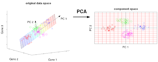
PCA is commonly used in:
- Reducing the number of features in high-dimensional datasets while preserving as much variance as possible.
- Visualizing high-dimensional data in 2D or 3D.
- Noise filtering and data compression.
- Feature extraction and selection.
Why PCA?
In many machine learning tasks, data often has a high number of dimensions, making computation expensive and difficult to interpret. For example, a movie recommender system might have thousands of features per movie (genre, director, actors, ratings, etc.). By using PCA, we can reduce this number to a smaller set of components that capture the most important patterns in the data.
How PCA Works
PCA involves the following steps:
- Standardization: The data is centered by subtracting the mean and scaled to have unit variance.
- Covariance Matrix Computation: A covariance matrix is computed to understand feature relationships.
- Eigenvalue and Eigenvector Computation: The eigenvalues and eigenvectors of the covariance matrix are found.
- Choosing Principal Components: The eigenvectors corresponding to the largest eigenvalues are selected as the principal components.
- Transforming the Data: The original data is projected onto the new principal component axes.
Mathematical Foundation of PCA
Step 1: Standardization
Since PCA relies on variance, the data should be standardized to have a mean of zero and unit variance:
$$ x’ = \frac{x - \mu}{\sigma} $$
where:
- $x$ is the original feature,
- $\mu$ is the mean of the feature,
- $\sigma$ is the standard deviation.
Step 2: Compute the Covariance Matrix
The covariance matrix captures relationships between different features:
$$ C = \frac{1}{n} X^T X $$
where $X$ is the standardized data matrix.
Step 3: Eigenvalues and Eigenvectors
PCA identifies principal components by computing eigenvalues and eigenvectors of the covariance matrix:
$$ C v = \lambda v $$
where:
- $\lambda$ are eigenvalues (variance captured by each principal component),
- $v$ are eigenvectors (principal component directions).
Step 4: Project Data onto Principal Components
Data is transformed into the new coordinate system:
$$ Z = X V_k $$
where $V_k$ contains the top $k$ eigenvectors.
PCA Visualization Example
We will visualize a dataset before and after applying PCA.
import numpy as np
import matplotlib.pyplot as plt
from sklearn.decomposition import PCA
from mpl_toolkits.mplot3d import Axes3D
# 3D veriyi oluşturma
np.random.seed(42)
n_samples = 100
mean1 = [2, 2, 2]
cov1 = [[1, 0.5, 0.2], [0.5, 1, 0.1], [0.2, 0.1, 1]]
data1 = np.random.multivariate_normal(mean1, cov1, n_samples)
mean2 = [5, 5, 5]
cov2 = [[1, -0.3, 0.1], [-0.3, 1, -0.2], [0.1, -0.2, 1]]
data2 = np.random.multivariate_normal(mean2, cov2, n_samples)
X = np.concatenate((data1, data2))
y = np.concatenate((np.zeros(n_samples), np.ones(n_samples)))
# 3D veriyi görselleştirme
fig = plt.figure(figsize=(12, 6))
ax = fig.add_subplot(121, projection='3d')
ax.scatter(X[:, 0], X[:, 1], X[:, 2], c=y, cmap='coolwarm', edgecolors='k')
ax.set_xlabel('X')
ax.set_ylabel('Y')
ax.set_zlabel('Z')
ax.set_title('Original 3D Data')
# PCA uygulama
pca = PCA(n_components=2)
X_pca = pca.fit_transform(X)
# 2D veriyi görselleştirme
ax2 = fig.add_subplot(122)
ax2.scatter(X_pca[:, 0], X_pca[:, 1], c=y, cmap='coolwarm', edgecolors='k')
ax2.set_xlabel('Principal Component 1')
ax2.set_ylabel('Principal Component 2')
ax2.set_title('Data After PCA (2D)')
plt.tight_layout()
plt.show()
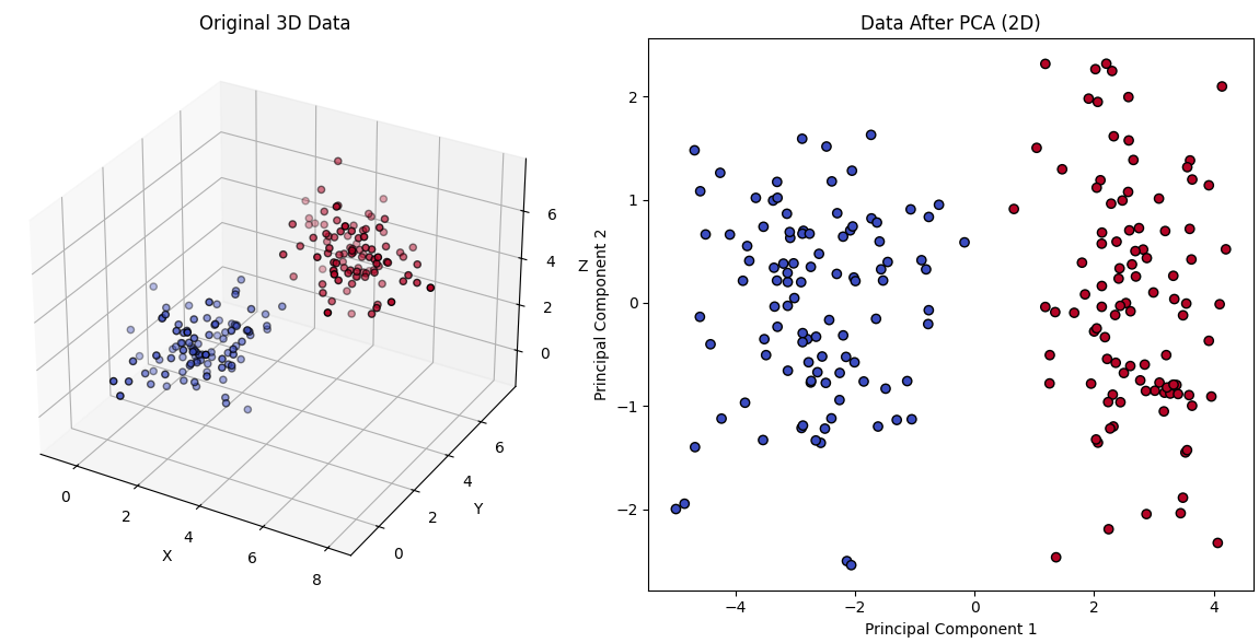
- The first plot shows the original dataset.
- The second plot shows the data projected onto the two principal components.
- PCA effectively captures the main variance in the data while reducing its dimensionality.
Conclusion
PCA is a fundamental technique for dimensionality reduction and data visualization. By identifying principal components, it helps uncover patterns, reduce noise, and improve machine learning model efficiency. However, PCA assumes linearity and may not perform well for highly non-linear data, where techniques like t-SNE or UMAP might be better alternatives.
Reinforcement Learning
- What is Reinforcement Learning?
- Markov Decision Process (MDP)
- State-Action Value Function ($Q(s,a)$)
- Bellman Equation
- Stochastic Environment (Randomness in RL)
- Continuous State vs. Discrete State
- Lunar Lander Example
- $ \varepsilon $-Greedy Policy
- Mini-Batch Learning in Reinforcement Learning
What is Reinforcement Learning?
Reinforcement Learning (RL) is a machine learning paradigm where an agent learns to make sequential decisions by interacting with an environment to maximize a cumulative reward. Unlike supervised learning, where labeled data is provided, RL relies on trial and error, receiving feedback in the form of rewards or penalties.
Key Characteristics of Reinforcement Learning:
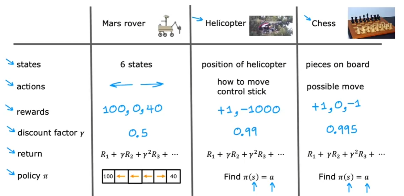
- Agent: The entity making decisions (e.g., a robot, a self-driving car, or an AI player in a game).
- Environment: The external system with which the agent interacts.
- State (s): A representation of the current situation of the agent in the environment.
- Action (a): A choice made by the agent at a given state.
- Reward (R): A numerical value given to the agent as feedback for its actions.
- Policy ( $ \pi$ ): A strategy that maps states to actions.
- Return (G): The cumulative reward collected over time.
- Discount Factor ( $ \gamma $ ): A value between 0 and 1 that determines the importance of future rewards.
Mars Rover Example
Let’s illustrate RL concepts using a Mars Rover example. Imagine a rover exploring a 1D terrain with six grid positions:
Each position is numbered from 1 to 6. The rover starts at position 4, and it can move left (-1) or right (+1). The goal is to maximize its rewards, which are given at positions 1 and 6:
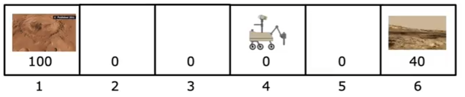
- Position 1 reward: 100 (e.g., a research station with supplies)
- Position 6 reward: 40 (e.g., a safe resting point)
- Other positions reward: 0
States, Actions, and Rewards
| State | Possible Actions | Reward |
|---|---|---|
| 1 | Move right (+1) | 100 |
| 2 | Move left (-1), Move right (+1) | 0 |
| 3 | Move left (-1), Move right (+1) | 0 |
| 4 (Start) | Move left (-1), Move right (+1) | 0 |
| 5 | Move left (-1), Move right (+1) | 0 |
| 6 | Move left (-1) | 40 |
- The agent (rover) must decide which direction to move.
- The state is the current position of the rover.
- The action is moving left or right.
- The reward depends on reaching the goal states (1 or 6).
How the Rover Decides Where to Go
The rover’s decision is based on maximizing its expected future rewards. Since it has two possible goal positions (1 and 6), it must evaluate different strategies. The rover should consider the following:
-
Immediate Reward Strategy
- If the rover focuses only on immediate rewards, it will move randomly, as most positions (except 1 and 6) have a reward of 0.
- This strategy is not optimal because it doesn’t take future rewards into account.
-
Short-Term Greedy Strategy
- If the rover chooses the nearest reward, it will likely go to position 6 since it’s closer than position 1.
- However, this might not be the best long-term decision.
-
Long-Term Reward Maximization
- The rover must evaluate how much discounted future reward it can accumulate.
- Even though position 6 has a reward of 40, position 1 has a much higher reward (100).
- If the rover can reliably reach position 1, it should favor this route, even if it takes more steps.
To formalize this, the rover can compute the expected return G for each possible path, considering the discount factor ($ \gamma $).
Discount Factor ($ \gamma $) and Expected Return
The discount factor $ \gamma $ determines how much future rewards are valued relative to immediate rewards. If $ \gamma = 1 $, all future rewards are considered equally important. If $ \gamma = 0.9 $, future rewards are slightly less important than immediate rewards.
For example, if the rover follows a path where it expects to reach position 1 in 3 steps and receive 100 reward, the discounted return is:
$$ G = 100 \times \gamma^3 = 100 \times 0.9^3 = 72.9 $$
If it reaches position 6 in 2 steps and receives 40 reward, the return is:
$$ G = 40 \times \gamma^2 = 40 \times 0.9^2 = 32.4 $$
Since 72.9 is greater than 32.4, the rover should prioritize going to position 1, even though it is farther away.
Policy ($ \pi $)
A policy ($ \pi $) defines the strategy of the rover: for each state, it dictates which action to take. Possible policies include:
- Greedy policy: Always moves towards the highest reward state immediately.
- Exploratory policy: Sometimes tries new actions to find better strategies.
- Discounted return policy: Balances short-term and long-term rewards.
If the rover follows an optimal policy, it should compute the total expected reward for every possible action and pick the one that maximizes its long-term return.
Markov Decision Process (MDP)
Reinforcement Learning problems are often modeled as Markov Decision Processes (MDPs), which are defined by:
- Set of States (S): $ s_1, s_2, …, s_n $
- Set of Actions (A): $ a_1, a_2, …, a_m $
- Transition Probability (P): Probability of moving from one state to another given an action $ P(s’ | s, a) $
- Reward Function (R): Defines the reward received when moving from $ s $ to $ s’ $
- Discount Factor ($ \gamma $): Determines the importance of future rewards.
In our Mars Rover example:
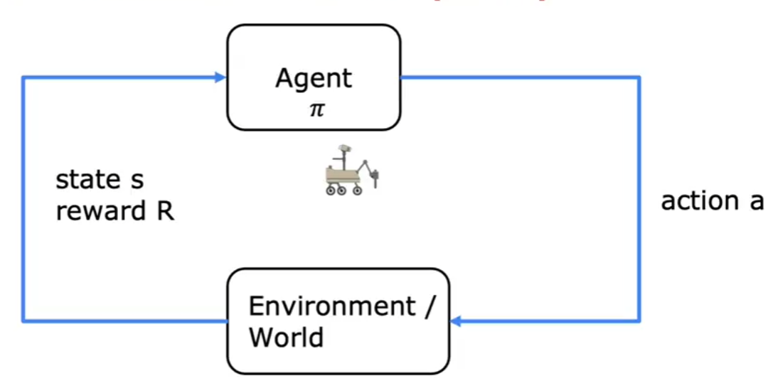
- States (S): {1, 2, 3, 4, 5, 6}
- Actions (A): {Left (-1), Right (+1)}
- Transition Probabilities (P): Deterministic (e.g., if the rover moves right, it always reaches the next state)
- Reward Function (R):
- $ R(1) = 100 $, $ R(6) = 40 $, $ R(2,3,4,5) = 0 $
- Discount Factor ($ \gamma $): $ 0.9 $ (assumed)
State-Action Value Function ($Q(s,a)$)
The State-Action Value Function, denoted as $Q(s,a)$, represents the expected return when starting from state $s$, taking action $a$, and then following a policy $\pi$. Formally:
$$ Q(s,a) = \mathbb{E} \big[ G_t \mid S_t = s, A_t = a \big] $$
This function helps the agent determine which action will lead to the highest reward in a given state.
Applying to Mars Rover
Using our Mars rover example, we can estimate $Q(s,a)$ values for each state-action pair. Suppose:
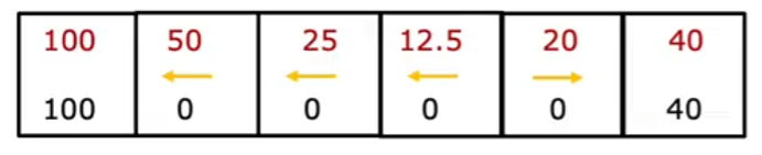
- $Q(4, \text{left}) = 25$
- $Q(4, \text{right}) = 20$
- $Q(5, \text{right}) = 40$
- $Q(3, \text{left}) = 50$
The rover should always select the action with the highest $Q$ value to maximize rewards.
Bellman Equation
The Bellman Equation provides a recursive relationship for computing value functions in reinforcement learning. It expresses the value of a state in terms of the values of successor states.
Understanding the Bellman Equation
In reinforcement learning, an agent makes decisions in a way that maximizes future rewards. However, since future rewards are uncertain, we need a way to estimate them efficiently. The Bellman equation helps us do this by breaking down the value of a state into two components:
- Immediate Reward ($R(s,a)$): The reward received by taking action $a$ in state $s$.
- Future Rewards ($V(s’)$): The expected value of the next state $s’$, weighted by the probability of reaching that state.
The Bellman equation is written as:
$$ V(s) = \max_a \Big[ R(s,a) + \gamma \sum_{s’} P(s’ | s,a) V(s’) \Big] $$
where:
- $V(s)$: The value of state $s$.
- $R(s,a)$: The immediate reward for taking action $a$ in state $s$.
- $\gamma$: The discount factor ($0 \leq \gamma \leq 1$), which determines how much future rewards are considered.
- $P(s’ | s,a)$: The probability of reaching state $s’$ after taking action $a$.
- $V(s’)$: The value of the next state $s’$.
Example Calculation for Mars Rover
Let’s assume:
- Moving from
4to3has a reward of-1. - Moving from
4to5has a reward of-1. - Position
1has a reward of100.
For $s=4$:
$$ V(4) = \max \big[ -1 + \gamma V(3), -1 + \gamma V(5) \big] $$
If we assume $V(3) = 50$ and $V(5) = 30$, and a discount factor $\gamma = 0.9$, we compute:
$$ V(4) = \max \big[ -1 + 0.9 \times 50, -1 + 0.9 \times 30 \big] $$
$$ V(4) = \max \big[ -1 + 45, -1 + 27 \big] $$
$$ V(4) = \max [44, 26] = 44 $$
Thus, the optimal value for state 4 is 44, meaning the agent should prefer moving left toward 3.
Intuition Behind the Bellman Equation
- The Bellman equation decomposes the value of a state into its immediate reward and the expected future reward.
- It allows us to compute values iteratively: we start with rough estimates and refine them over time.
- It helps in policy evaluation—determining how good a given policy is.
- It forms the foundation for Dynamic Programming methods like Value Iteration and Policy Iteration.
Stochastic Environment (Randomness in RL)
In real-world applications, environments are often stochastic, meaning actions do not always lead to the same outcome.
Stochasticity in the Mars Rover Example
Suppose the Mars rover’s motors sometimes malfunction, causing it to move in the opposite direction with a small probability (e.g., 10% of the time). Now, the transition dynamics include:
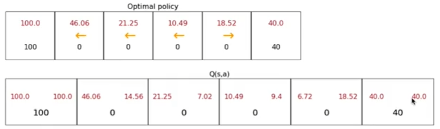
- $P(s’ = 5 | s = 4, a = \text{right}) = 0.9$
- $P(s’ = 3 | s = 4, a = \text{right}) = 0.1$
This randomness makes decision-making more challenging. Instead of just considering rewards, the rover must now account for expected rewards and the probability of ending up in different states.
Impact on Decision-Making
With stochastic environments, deterministic policies (always taking the best action) may not be optimal. Instead, an exploration-exploitation balance is needed:
- Exploitation: Following the best-known action based on past experience.
- Exploration: Trying new actions to discover potentially better rewards.
This concept is central to algorithms like Q-Learning and Policy Gradient Methods, which we will discuss in future sections.
Continuous State vs. Discrete State
In reinforcement learning, states can be either discrete or continuous. A discrete state means that the number of possible states is finite and well-defined, whereas a continuous state implies an infinite number of possible states.
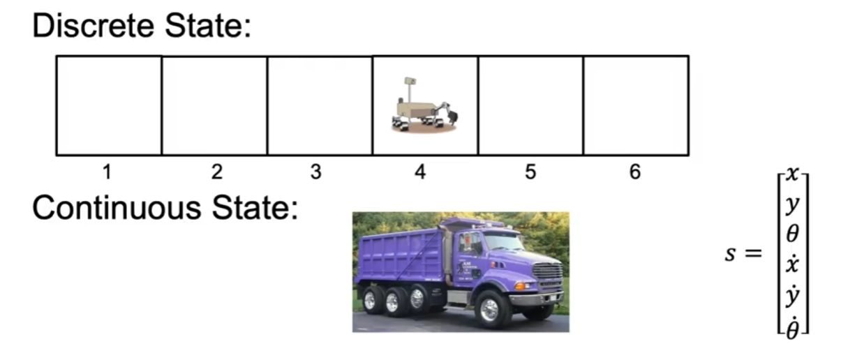
For example, consider our Mars Rover example with six possible states. The rover can be in any one of these six states at any given time, making it a discrete state environment. However, if we consider a truck driving on a highway, its position, speed, angle, and other attributes can take an infinite number of values, making it a continuous state environment.
Continuous state spaces are often approximated using function approximators like neural networks to generalize over an infinite number of states efficiently.
Lunar Lander Example
A classic reinforcement learning problem is the Lunar Lander, where the objective is to safely land a spacecraft on the surface of a planet. The agent (lander) interacts with the environment by selecting one of four possible actions:
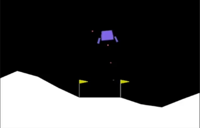
- Do Nothing: No thrust is applied.
- Left Thruster: Applies force to move left.
- Right Thruster: Applies force to move right.
- Main Thruster: Applies force to slow descent.
Rewards and Penalties:
The environment provides feedback through rewards and penalties:
- Soft Landing: +100 reward
- Crash Landing: -100 penalty
- Firing Main Engine: -0.3 penalty (fuel consumption)
- Firing Side Thrusters: -0.1 penalty (fuel consumption)
State Representation
The state of the lunar lander can be represented as:
$$ s = [x, y, \theta, l, r, x’, y’, \theta’] $$
where:
- $ x, y $ : Position of the lander
- $ \theta $ : Orientation (tilt angle)
- $ l, r $ : Contact with left and right landing pads (binary values)
- $ x’, y’ $ : Velocities in x and y directions
- $ \theta’ $ : Angular velocity
The policy function $ \pi(s) $ determines which action to take given the current state.
Deep Q-Network (DQN) Neural Network for Lunar Lander
To approximate the optimal policy, we use a deep neural network. The network takes the 8-dimensional state vector as input and predicts Q-values for each of the four actions.
Network Architecture:
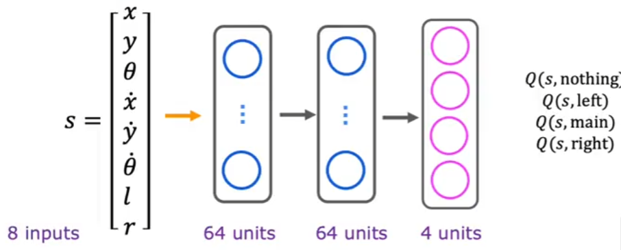
- Input Layer (8 neurons): Corresponds to $ x, y, \theta, l, r, x’, y’, \theta’ $
- Two Hidden Layers (64 neurons each, ReLU activation)
- Output Layer (4 neurons): Represents the Q-values for the four possible actions
The output neurons correspond to:
- $ Q(s, \text{do nothing}) $
- $ Q(s, \text{main thruster}) $
- $ Q(s, \text{right thruster}) $
- $ Q(s, \text{left thruster}) $
The network is trained using the Bellman equation to minimize the difference between predicted and actual Q-values.
$ \varepsilon $-Greedy Policy
In reinforcement learning, an agent must balance exploration (trying new actions) and exploitation (choosing the best-known action). The $ \varepsilon $-greedy policy is a common approach to achieve this balance:
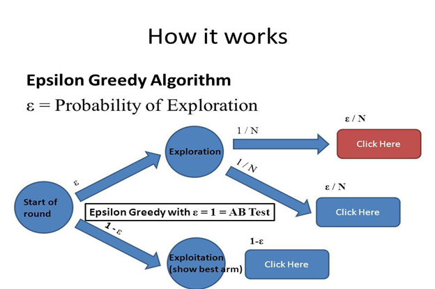
- With probability $ \varepsilon $, take a random action (exploration).
- With probability $ 1 - \varepsilon $, take the action with the highest Q-value (exploitation).
Initially, $ \varepsilon $ is set to a high value (e.g., 1.0) to encourage exploration and gradually decays over time.
Mini-Batch Learning in Reinforcement Learning
In deep reinforcement learning, we use mini-batch learning to improve training efficiency and stability.
Why Mini-Batch Learning?
- Prevents large updates from a single experience (stabilizes training).
- Helps break the correlation between consecutive experiences (improves generalization).
- Allows efficient GPU computation (faster convergence).
How It Works:
- Store experiences (state, action, reward, next state) in a replay buffer.
- Sample a mini-batch of experiences.
- Compute target Q-values using the Bellman equation.
- Perform a gradient descent update on the Q-network.
Mini-batch learning makes reinforcement learning more robust and prevents overfitting to recent experiences.
Content
∴
I completed the Deep Learning Specialization by taking detailed notes and summarizing critical concepts for future reference.
Stanford University & DeepLearning.AI
Course & Note Overview
This repository contains my personal, rigorous study notes taken throughout the 5 courses of the Deep Learning Specialization. Rather than standard lecture transcripts, these notes focus on deep mathematical derivations, architectural intuition, practical debugging strategies, and production considerations across modern deep learning pipelines.
| # | Course | Core Focus & Note Contents |
|---|---|---|
| 1 | Neural Networks and Deep Learning | Vectorized forward/backpropagation derivations, activation functions, loss optimization, and multi-layer architecture fundamentals. |
| 2 | Improving Deep Neural Networks | Practical hyperparameter tuning, regularization (Dropout, L2), optimization algorithms (Momentum, RMSprop, Adam), and Batch Normalization. |
| 3 | Structuring Machine Learning Projects | Diagnostic frameworks, error analysis, train/dev/test distribution mismatch handling, and end-to-end ML strategy. |
| 4 | Convolutional Neural Networks | Convolution arithmetic, classic/modern backbones (ResNet, MobileNet), object detection (YOLO, Anchor boxes), semantic segmentation (U-Net), and neural style transfer. |
| 5 | Sequence Models | Temporal modeling with RNNs, GRUs, and LSTMs, attention mechanisms, Transformer architectures, NLP embeddings, and sequence-to-sequence workflows. |
— emreaslan —
Computer Vision and Edge Detection
- Computer Vision
- Edge Detection
Computer Vision
Introduction to Computer Vision
Computer Vision is a field of artificial intelligence (AI) that enables machines to interpret and understand visual information from the world. It encompasses tasks such as image recognition, object detection, and segmentation.
Real-World Applications
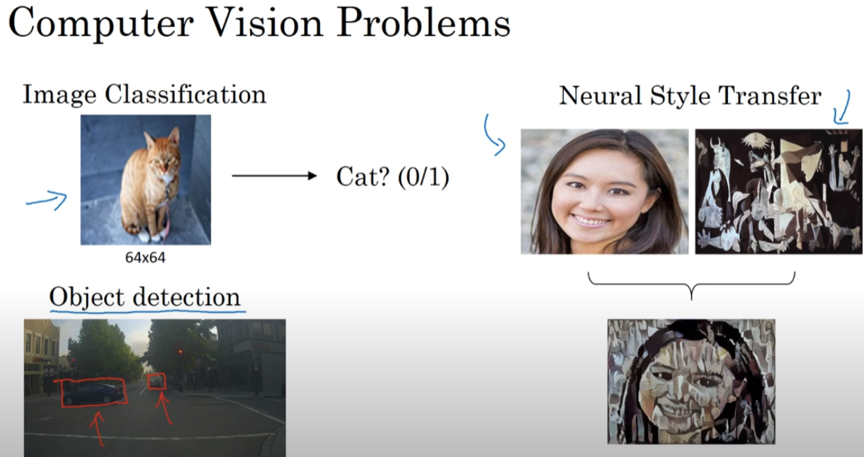
- Facial Recognition: Used in security systems and social media tagging.
- Medical Imaging: Helps in detecting diseases using X-rays, MRIs, and CT scans.
- Autonomous Vehicles: Enables self-driving cars to recognize objects and road signs.
- Industrial Automation: Used for defect detection in manufacturing.
Fundamental Concepts
- Pixels: The smallest unit in an image.
- Grayscale and Color Images: Difference between single-channel and multi-channel images.
- Resolution: Number of pixels in an image.
- Image Representation: Images as matrices of pixel values.
Mathematical Formulation
An image can be represented as a matrix:
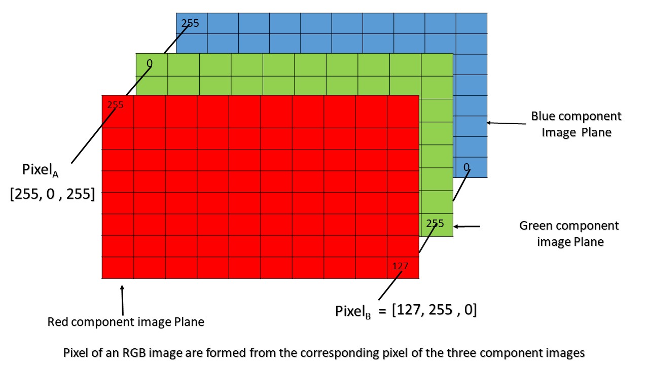
$$ I(x, y) \in \mathbb{R}^{m \times n \times c} $$
where $m$ and $n$ represent height and width, and $c$ represents the number of color channels (1 for grayscale, 3 for RGB images).
Edge Detection
Why Use Convolution for Edge Detection?
Edge detection aims to find points in an image where the intensity changes sharply. These points often correspond to boundaries of objects, texture changes, or discontinuities in depth. To detect these changes, we apply convolution operations with specific filters.
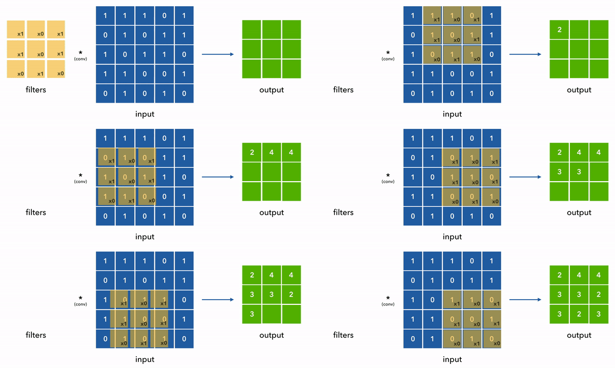
Convolution is a mathematical operation that helps us apply a small matrix (called a filter or kernel) across the entire image to detect specific patterns like edges.
What Does a Filter Do?
A filter is essentially a small grid of numbers (e.g., $3x3$) that slides across the image and emphasizes certain features:
- Edge filters highlight intensity changes
- Blur filters smooth the image
- Sharpening filters enhance details
In edge detection, filters are designed to detect high spatial frequency changes—essentially, edges.
Mathematical Example
$$ I = \left[ \begin{array}{cccccc} 12 & 15 & 14 & 10 & 9 & 10 \ 18 & 20 & 22 & 17 & 14 & 12 \ 24 & 28 & 30 & 26 & 20 & 18 \ 30 & 33 & 35 & 32 & 28 & 25 \ 22 & 25 & 28 & 24 & 22 & 20 \ 15 & 17 & 19 & 18 & 16 & 15 \end{array} \right] $$
We apply a vertical Sobel filter $ K_v $:
$$ K_v = \left[ \begin{array}{ccc} -1 & 0 & 1 \ -2 & 0 & 2 \ -1 & 0 & 1 \end{array} \right] $$
This filter detects vertical edges by highlighting horizontal intensity transitions.
Step-by-Step Convolution (No Padding, Stride = 1)
Let’s compute the top-left value of the output matrix. We place the filter on the top-left 3x3 window of ( I ):
Window:
$$ \left[ \begin{array}{ccc} 12 & 15 & 14 \ 18 & 20 & 22 \ 24 & 28 & 30 \end{array} \right] $$
Element-wise multiplication and sum:
$$ (-1 \cdot 12) + (0 \cdot 15) + (1 \cdot 14) + (-2 \cdot 18) + (0 \cdot 20) + (2 \cdot 22) + (-1 \cdot 24) + (0 \cdot 28) + (1 \cdot 30) $$
$$ = -12 + 0 + 14 - 36 + 0 + 44 - 24 + 0 + 30 = 16 $$
So, the top-left value of the output matrix is 16.
Second Convolution Step (Next to Right)
New window (move filter one step to the right):
$$ \left[ \begin{array}{ccc} 15 & 14 & 10 \ 20 & 22 & 17 \ 28 & 30 & 26 \end{array} \right] $$
Apply the same operation:
$$ (-1 \cdot 15) + (0 \cdot 14) + (1 \cdot 10) + (-2 \cdot 20) + (0 \cdot 22) + (2 \cdot 17) + (-1 \cdot 28) + (0 \cdot 30) + (1 \cdot 26) $$
$$ = -15 + 0 + 10 - 40 + 0 + 34 - 28 + 0 + 26 = -13 $$
So, second value is -13.
Full Output Matrix (4x4)
After sliding the filter across the 6x6 image, we get the 4x4 output:
$$ I * K_v = \left[ \begin{array}{cccc} 16 & -13 & -25 & -26 \ 20 & -11 & -22 & -24 \ 12 & -8 & -18 & -16 \ 4 & -5 & -9 & -8 \end{array} \right] $$
This matrix highlights the vertical edges in the original image—areas where pixel intensities change most dramatically from left to right.
The result of convolving the image with these filters gives us areas of strong gradient—edges.
Key Insight:
Filters translate the idea of change in pixel values into a computable quantity.
Edge Detection Techniques
1. Sobel Operator
- Combines Gaussian smoothing and differentiation.
- Horizontal ($ G_x $) and vertical ($ G_y $) gradients are calculated using predefined 3x3 kernels.
$$ 3 x 3 \text(Sobel Kernels)$$
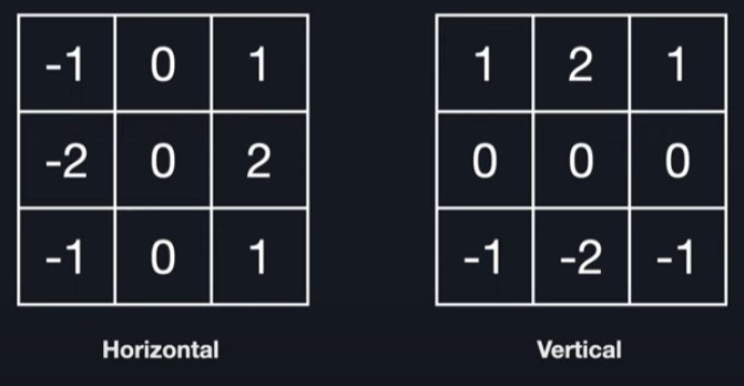
- The gradient magnitude is: $$ G = \sqrt{G_x^2 + G_y^2}, \quad \theta = \tan^{-1}\left(\frac{G_y}{G_x}\right) $$
- Commonly used due to simplicity and noise resistance.
- Watch this youtube video
2. Prewitt Operator
- Similar to Sobel, but with uniform weights.
$$ 3 x 3 \text(Prewitt Kernels)$$
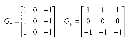
- Slightly less sensitive to noise compared to Sobel.
3. Laplacian of Gaussian (LoG)
- A second derivative method.
- Detects edges by identifying zero-crossings after applying the Laplacian to a Gaussian-smoothed image.
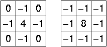
- Equation: $$ \nabla^2 I = \frac{\partial^2 I}{\partial x^2} + \frac{\partial^2 I}{\partial y^2} $$
- Sensitive to noise, hence Gaussian smoothing is applied first.
4. Canny Edge Detection
A multi-stage algorithm designed for optimal edge detection:
- Gaussian Filtering: Noise reduction.
- Gradient Calculation: Using Sobel filters.
- Non-Maximum Suppression: Thinning the edges.
- Double Thresholding: Classify edges as strong, weak, or non-edges.
- Hysteresis: Connect weak edges to strong ones if they are adjacent.
Canny is widely used in practice for its high accuracy and low false detection.
5. Difference of Gaussians (DoG)
- Approximates the LoG by subtracting two Gaussian-blurred images: $$ DoG = G_{\sigma_1} * I - G_{\sigma_2} * I $$
- Faster to compute than LoG.
- Used in blob detection and feature matching.
Convolutional Operations
Padding
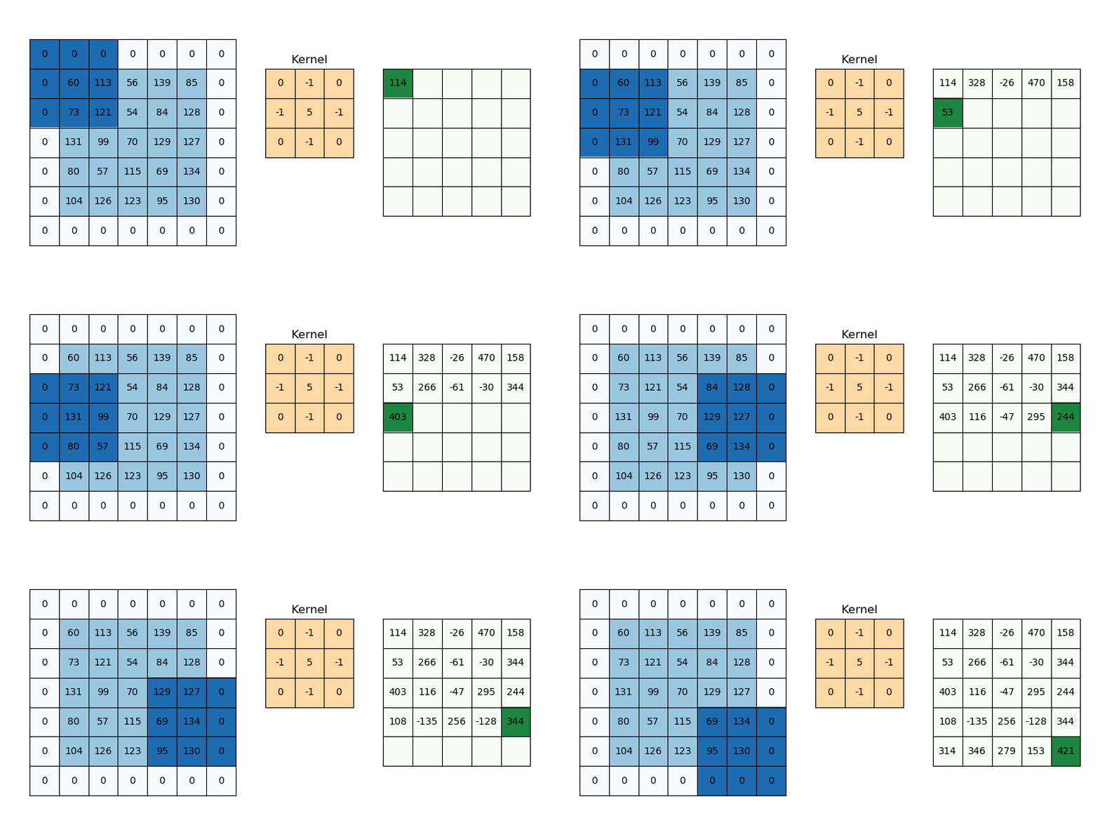
Why Padding is Needed
When applying convolution, the output image shrinks unless we pad it. This is a problem when building deep networks where spatial dimensions shrink after each convolution.
Without Padding:
$$ \text{Output size} = n - f + 1 $$
Where:
- $n$: input size
- $f$: filter size
Example
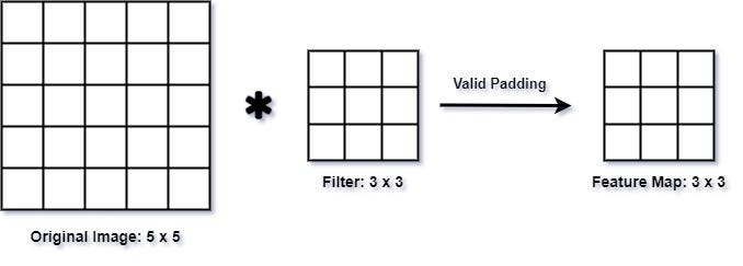
In this image:
- $n$: input size = $5$
- $f$: filter size = $3$
$$ \text{Output size} = n - f + 1 $$
$$ \text{Output size} = 5 - 3 + 1 $$
$$ \text{Output size} = 3 $$
With Padding ($p$):
$$ \text{Output size} = n + 2p - f + 1 $$
Where:
- $n$: input size
- $f$: filter size
- $p$: padding size
Example
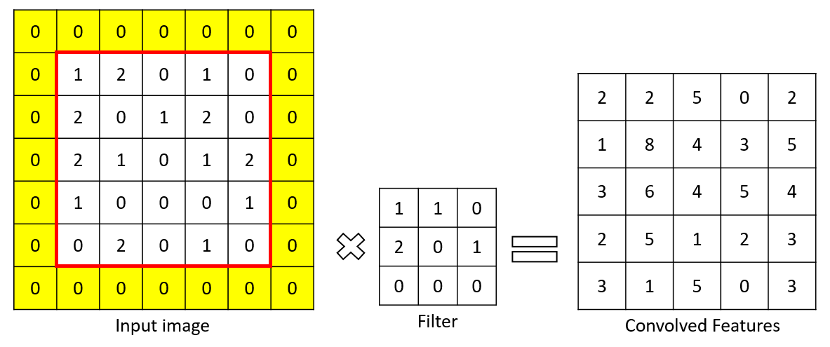
In this image:
- $n$: input size = $6$
- $f$: filter size = $3$
- $p$: padding size = $1$
$$ \text{Output size} = n + 2p - f + 1 $$
$$ \text{Output size} = 6 + (2\cdot 1) - 3 + 1 $$
$$ \text{Output size} = 6 $$
Types of Padding
- Valid Padding (no padding): Output is smaller.
- Same Padding (zero padding): Output size equals input size.
Real-World Analogy
Imagine scanning a photo with a magnifying glass: without padding, you can’t examine the borders. Padding extends the image so that every pixel gets equal attention.
Strided Convolutions
What is Stride?
Stride is the number of pixels the filter moves at each step.
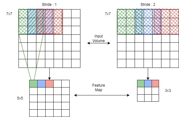
- Stride = 1: Normal convolution (moves 1 pixel at a time)
- Stride = 2: Downsampling (moves 2 pixels at a time)
Output Size Formula
$$ \text{Output size} = \left\lfloor \frac{n + 2p - f}{s} \right\rfloor + 1 $$
Where:
- $n$: input size
- $f$: filter size
- $s$: stride
- $p$: padding
Visual Example
If stride = 2, the filter skips every alternate pixel, effectively reducing the spatial size of the output.
Convolutions Over Volume
From 2D to 3D
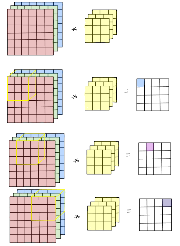
In RGB images, we have 3 channels: Red, Green, and Blue. Thus, a convolutional layer operates over 3D volumes.
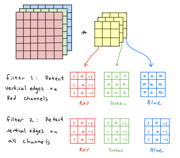
Input Dimensions:
$$ (n_H, n_W, n_C) $$
- $n_H$: Height
- $n_W$: Width
- $n_C$: Channels (e.g., 3 for RGB)
Filter Dimensions:
$$ (f_H, f_W, n_C) $$
- Number of filters: $n_F$
Output Volume:
$$ (n_H’, n_W’, n_F) $$
- Each filter creates a 2D activation map, stacked together to form the output volume.
Practical Example
Let’s say you have a (6, 6, 3) image, and you apply 2 filters of size (3, 3, 3):
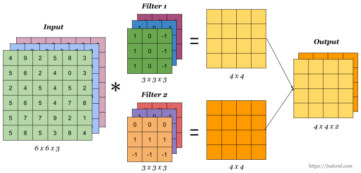
- Output shape: (4, 4, 2) (assuming valid padding, stride=1)
CNN Architecture and Examples
1. One Layer of a Convolutional Network
A Convolutional Neural Network (CNN) is typically composed of three types of layers:
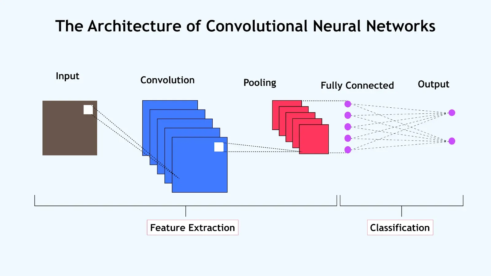
- Convolutional layers: Apply filters to extract spatial features.
- Pooling layers: Downsample feature maps to reduce computation.
- Fully connected layers: Perform final classification or regression.
Each layer transforms the input volume into an output volume through learnable parameters or fixed operations.
Layer Types of CNN
1. Convolutional Layers
Purpose:
To extract spatial features such as edges, textures, and patterns by sliding filters over the input image or feature map.
How it works:
- A filter (or kernel) of size $f \times f$ slides over the input.
- At each location, an element-wise multiplication is performed between the filter and the part of the input it overlaps.
- The results are summed to produce a single number in the output feature map.
Mathematical Operation:
Let the input be $X \in \mathbb{R}^{n_H \times n_W \times n_C}$ and the filter be $W \in \mathbb{R}^{f \times f \times n_C}$.
$$ Z_{i,j} = \sum_{m=0}^{f-1} \sum_{n=0}^{f-1} \sum_{c=0}^{n_C-1} X_{i+m,j+n,c} \cdot W_{m,n,c} + b $$
Example:
Input: $5 \times 5$ grayscale image with $3 \times 3$ filter:
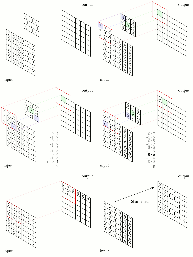
As the filter slides across the input, it detects vertical and horizontal edges by producing high activation in regions with strong center transitions.
2. Pooling Layers
Purpose:
To reduce the spatial dimensions (height and width) of the feature maps, thereby:
- Reducing the number of parameters and computation
- Controlling overfitting
- Making the model invariant to small translations in the input
Types:
Max Pooling:
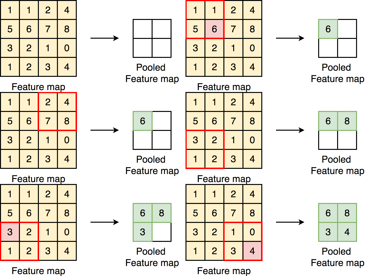
Selects the maximum value in each region.
Average Pooling:
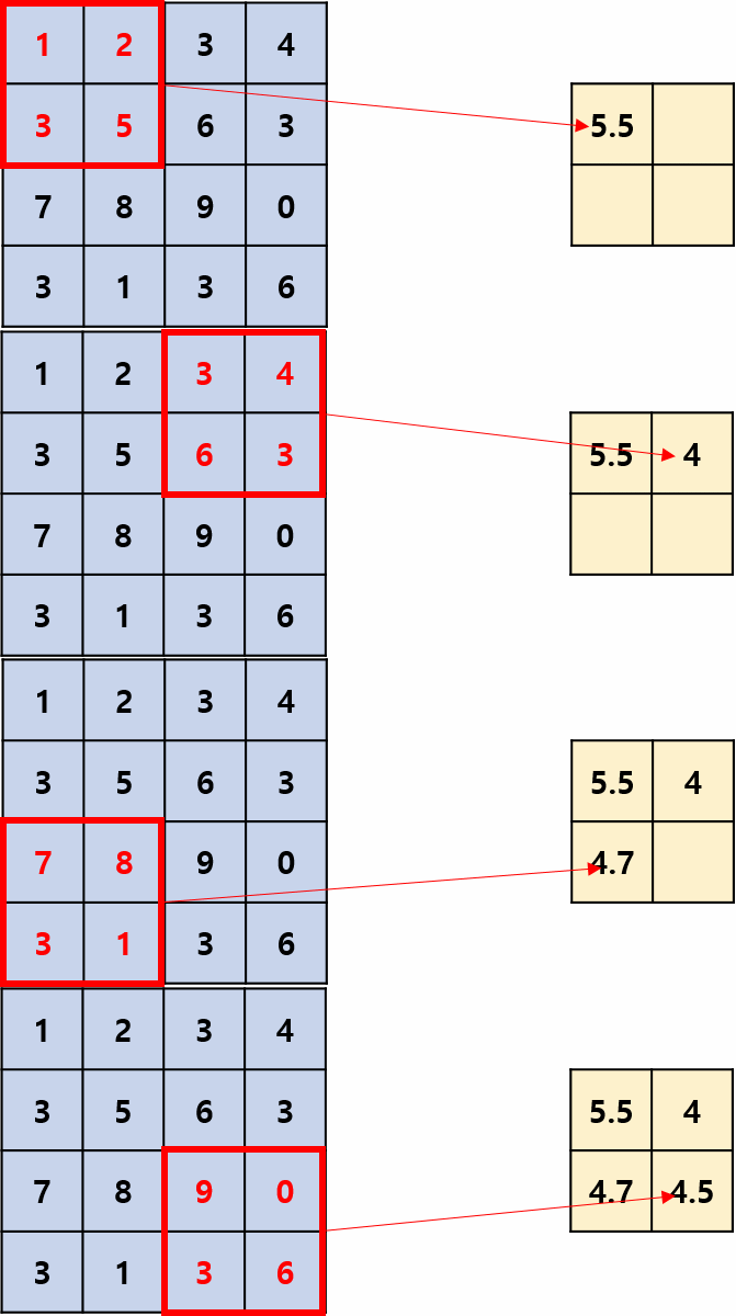
Takes the average of values in each region.
3. Fully Connected Layers
To connect every neuron in one layer to every neuron in the next layer, performing the final classification or regression.
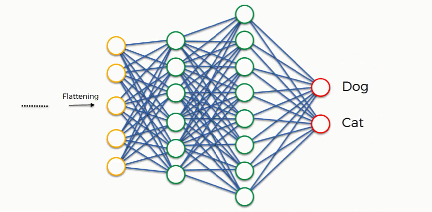
How it works:
- Takes the flattened output from the last convolutional/pooling layer
- Passes it through one or more dense layers
- Final layer often uses softmax for classification
Mathematical Form:
Given the input vector $x \in \mathbb{R}^n$, weights $W \in \mathbb{R}^{m \times n}$, and bias $b \in \mathbb{R}^m$:
$$ z = Wx + b $$
$$ a = g(z) \text{ where } g \text{ is an activation function (e.g., ReLU, Softmax)} $$
Example:
Let’s say we have a feature map output size of $5 \times 5 \times 16 = 400$ from the last pooling layer:
- FC1: 400 → 120 (ReLU)
- FC2: 120 → 84 (ReLU)
- FC3: 84 → 10 (Softmax, for 10-class classification)
These dense layers combine all the high-level features learned in the earlier layers and output a prediction.
Summary Table
| Layer Type | Role | Typical Parameters | Output Shape Transformation |
|---|---|---|---|
| Convolutional | Extract local spatial features | $f$, $s$, $p$, filters | $n_H \times n_W \times n_C \rightarrow n_{H’} \times n_{W’} \times n_{C’}$ |
| Pooling | Downsample feature maps | $f$, $s$ | $n_H \times n_W \times n_C \rightarrow n_{H’} \times n_{W’} \times n_C$ |
| Fully Connected | Final classification/regression | neurons per layer | $n \rightarrow m$ (vector size) |
These layers together form the foundation of Convolutional Neural Networks, enabling them to learn hierarchical representations from raw pixels to abstract concepts.
Notation and Terminology
- $ n_H, n_W $: height and width of the input volume
- $ n_C $: number of channels (depth)
- $ f $: filter size
- $ s $: stride
- $ p $: padding
- $ W^{[l]} $, $ b^{[l]} $: weights and biases at layer $ l $
Parameters and Learnable Components
- Weights ($ W $): Represent filters; shared spatially across the input.
- Biases ($ b $): One per filter.
- Activation ($ A $): Output of ReLU or other non-linear function.
Each neuron in a layer is connected only to a small region of the previous layer, leading to sparse interactions and parameter sharing.
3. CNN Example (Comprehensive Network)
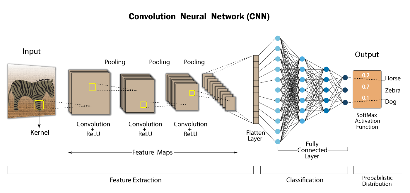
Why Convolutions?
Convolutional layers are the cornerstone of modern deep learning models in computer vision, replacing traditional fully connected layers in image tasks. This section explores why convolutions are used instead of dense layers, and what advantages they bring.
1. The Limitations of Fully Connected Layers for Images
a. Parameter Explosion
A fully connected (dense) layer connecting every pixel of an image to every neuron in the next layer requires a huge number of parameters.
Example:
- Input image size: $ 64 \times 64 \times 3 = 12,288 $
- Fully connected layer with 1000 neurons: $ \text{Parameters} = 12,288 \times 1000 = 12,288,000 $
This leads to high memory usage, overfitting risk, and long training times.
b. Ignores Spatial Structure
Dense layers treat input features independently and do not take advantage of the spatial locality of image data.
- A cat’s ear in the top-left and bottom-right corners are treated as unrelated by dense layers.
2. Benefits of Convolutional Layers
a. Sparse Interactions
Each output neuron is connected only to a small region of the input (called the receptive field).
- Fewer parameters
- Faster computations
Example:
- Using $ f = 5 $ instead of connecting all 12,288 pixels
b. Parameter Sharing
Same filter (weights) is applied across the entire image:
$$ Z[i, j] = \sum_{m=0}^{f-1} \sum_{n=0}^{f-1} W[m, n] \cdot X[i+m, j+n] + b $$
This results in drastic reduction in number of parameters and allows feature detection to be translation invariant.
c. Translation Equivariance
- If an object moves in the image, its feature map also moves.
- The model learns position-independent features — important for generalization.
Classic Networks: LeNet-5, AlexNet, VGG
- Why Look at Classic Networks?
- LeNet-5 (1998, Yann LeCun)
- AlexNet (2012, Alex Krizhevsky, Ilya Sutskever, Geoffrey Hinton)
- VGG Networks (2014, Visual Geometry Group, Oxford)
- Summary Table
- Final Thoughts
In the early stages of deep learning and computer vision, several foundational convolutional neural network (CNN) architectures shaped the field and enabled significant breakthroughs in image recognition. In this document, we explore three of the most historically significant and technically influential networks: LeNet-5, AlexNet, and VGG.
These architectures demonstrate the progression of CNN design from shallow, simple models to deeper, more powerful systems capable of scaling to large datasets like ImageNet.
Why Look at Classic Networks?
Understanding classic CNN architectures is essential for the following reasons:
- They introduce fundamental building blocks (e.g., convolutional layers, pooling layers, ReLU activation).
- They highlight challenges faced at different stages of deep learning evolution (e.g., overfitting, vanishing gradients).
- They provide insights into the design philosophy of modern deep architectures.
LeNet-5 (1998, Yann LeCun)
Overview
LeNet-5 was one of the earliest CNN models designed to recognize handwritten digits (e.g., MNIST dataset). It demonstrated the power of learned convolutional filters combined with a small number of parameters.
Architecture
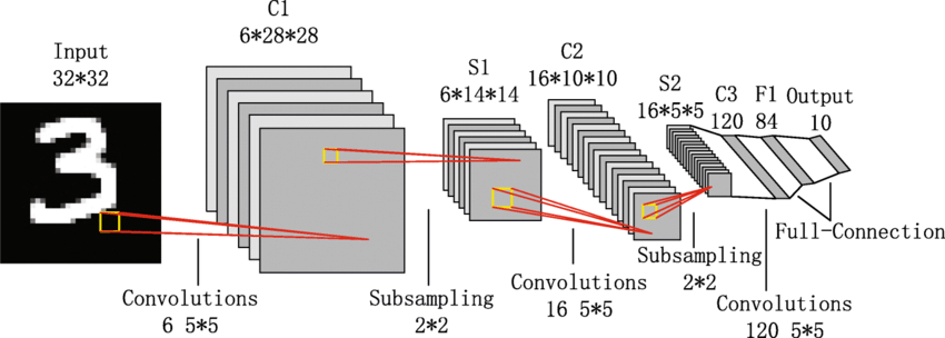
- Input: 32x32 grayscale image
- C1: Convolutional layer with 6 filters of size 5x5 → output: 28x28x6
- S2: Subsampling (average pooling) layer → output: 14x14x6
- C3: Convolutional layer with 16 filters → output: 10x10x16
- S4: Subsampling layer → output: 5x5x16
- C5: Fully connected convolutional layer → output: 120
- F6: Fully connected layer → output: 84
- Output: 10-class softmax layer
Parameters
LeNet uses shared weights, reducing the number of parameters compared to fully connected networks.
Insights
- Introduced the idea of local receptive fields, weight sharing, and subsampling.
- Excellent for small datasets but struggles with large-scale data due to its shallow depth.
AlexNet (2012, Alex Krizhevsky, Ilya Sutskever, Geoffrey Hinton)
Breakthrough
AlexNet marked the first major success of deep learning in the ImageNet Large Scale Visual Recognition Challenge (ILSVRC 2012), achieving top-5 error of 15.3%, compared to 26% for the runner-up.
Architecture
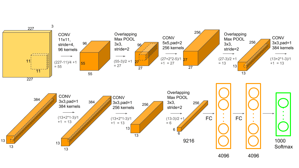
- Input: 224x224x3 RGB image
- Conv1: 96 filters of 11x11, stride 4 → 55x55x96
- MaxPool1: 3x3, stride 2 → 27x27x96
- Conv2: 256 filters of 5x5 → 27x27x256
- MaxPool2: 3x3 → 13x13x256
- Conv3: 384 filters of 3x3 → 13x13x384
- Conv4: 384 filters of 3x3 → 13x13x384
- Conv5: 256 filters of 3x3 → 13x13x256
- MaxPool3: 3x3 → 6x6x256
- FC6: Fully connected layer with 4096 neurons
- FC7: Fully connected layer with 4096 neurons
- FC8: 1000-way softmax layer
Key Innovations
- Used ReLU (Rectified Linear Unit) instead of sigmoid or tanh → faster training
- Introduced dropout for regularization
- Trained on two GPUs in parallel
Insights
- Showed the world that deep networks could outperform traditional machine learning models if trained with large datasets and GPUs.
VGG Networks (2014, Visual Geometry Group, Oxford)
VGG emphasized simplicity and depth: using small 3x3 filters and stacking them deeply to capture complex patterns.
Architecture (VGG-16)
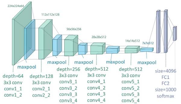
- Input: 224x224x3 RGB image
- Stack of 13 convolutional layers using 3x3 filters
- 5 max-pooling layers to reduce spatial dimensions
- 3 fully connected layers, with the last one as a softmax for classification
Example:
- Conv3-64 → Conv3-64 → MaxPool
- Conv3-128 → Conv3-128 → MaxPool
- Conv3-256 → Conv3-256 → Conv3-256 → MaxPool
- Conv3-512 → Conv3-512 → Conv3-512 → MaxPool
- Conv3-512 → Conv3-512 → Conv3-512 → MaxPool
- FC-4096 → FC-4096 → Softmax(1000)
Characteristics
- Consistent use of 3x3 filters simplifies the design and enables deeper networks
- Requires significant memory and computation (hundreds of millions of parameters)
Insights
- Demonstrated that depth is a key factor in improving CNN performance
- The architecture became a benchmark and inspired many follow-up models
Summary Table
| Model | Year | Input Size | Depth | Unique Aspects |
|---|---|---|---|---|
| LeNet-5 | 1998 | 32x32 | 7 | Local receptive fields, subsampling |
| AlexNet | 2012 | 224x224x3 | 8 | ReLU, dropout, GPU parallelism |
| VGG-16 | 2014 | 224x224x3 | 16 | Simplicity, 3x3 filters, depth |
Final Thoughts
These classic CNN architectures form the backbone of modern computer vision systems. Each contributed key architectural innovations that addressed specific challenges in training deep networks.
Understanding them allows us to appreciate the evolution of deep learning and to better design models suited for today’s massive data and compute resources.
Modern CNN Architectures: ResNet, Inception, MobileNet, EfficientNet
ResNet: Deep Residual Networks
As neural networks became deeper, researchers observed a counterintuitive phenomenon: deeper networks often performed worse during training and testing compared to shallower ones. This degradation was not due to overfitting but rather an optimization issue.
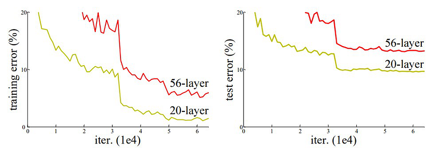
This problem is called the degradation problem. It shows that simply stacking more layers doesn’t guarantee better accuracy — instead, it often leads to higher training error. This contradicts our expectations, since deeper models should be able to represent more complex functions.
To address this, ResNet introduced the concept of residual learning.
Residual Learning: Core Idea
Instead of learning a direct mapping $ H(x) $, ResNet proposes to learn the residual function:
$$ F(x) = H(x) - x \Rightarrow H(x) = F(x) + x $$
This reformulation allows the network to focus on learning the difference between the input and output, which is often easier to optimize.
The output of a residual block is:
$$ \text{Output} = F(x, {W_i}) + x $$
where $ F(x, {W_i}) $ is the output from a few stacked layers (e.g., 2 Conv-BN-ReLU layers) and $ x $ is the original input. This addition is known as a skip connection or shortcut connection.
Here’s the basic structure of a Residual Block:
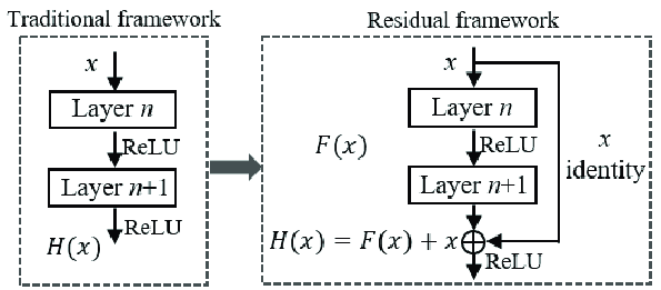
- If the input and output dimensions differ, a 1x1 convolution is used to match dimensions before addition.
- This structure allows gradients to flow more easily during backpropagation, mitigating the vanishing gradient problem.
Identity Shortcut Connection
This is the key innovation. By allowing the input to bypass intermediate layers, the model can preserve useful features, learn identity mappings when needed, and avoid overfitting.
Shortcut types:
- Identity shortcut: When input and output dimensions match
- Projection shortcut: 1x1 convolution used to match shapes
Why ResNets Work?
- Improved Gradient Flow: Easier to train deep networks due to unblocked gradient paths
- Easier Optimization: Residual mapping simplifies the learning process
- Deeper Networks: Can train very deep networks (e.g., ResNet-152) without degradation
- Better Generalization: Performs well across image classification, detection, segmentation
Forward and Backward Propagation
In a residual block, during forward propagation, the shortcut allows direct data flow from earlier layers. In backward propagation, the gradient can pass through both the residual path and shortcut connection, reducing gradient vanishing.
Let’s say the loss gradient is $ \partial L/\partial y $. Then:
$$ \frac{\partial L}{\partial x} = \frac{\partial L}{\partial y} \cdot (\frac{\partial F}{\partial x} + I) $$
Here, $ I $ is the identity matrix, ensuring that gradient doesn’t vanish even if $ \partial F/\partial x $ becomes small.
Real-World Analogy
Imagine you’re assembling a piece of furniture using instructions. Instead of reading and understanding every step from scratch (direct mapping), you compare each step with what you’ve already done (residual comparison). It’s easier to notice what’s missing and fix it.
Variants of ResNet
- ResNet-18, 34, 50, 101, 152: Increasing depth
- ResNeXt: Groups of convolutions
- Pre-activation ResNet: Moves BN and ReLU before convolutions
Inception and 1x1 Convolutions
Networks in Networks and 1x1 Convolutions
In 2014, the “Network in Network” architecture introduced the idea of using 1x1 convolutions — a surprisingly powerful and efficient technique in modern CNNs.
What is a 1x1 Convolution?
- A 1x1 convolution applies a filter of size $1×1$ across all input channels.
- Though the spatial dimension ($1x1$) seems trivial, it processes channel-wise information and mixes features across depth.
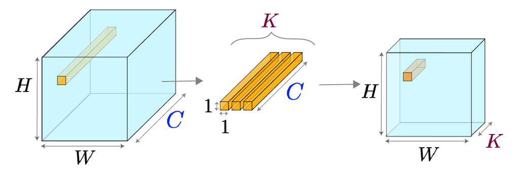
Let’s assume an input of shape $ H \times W \times C_{in}$. Applying $ N $ 1x1 filters produces an output of shape $ H \times W \times N $.
Why is it useful?
- Dimensionality Reduction: You can reduce the number of channels before applying computationally expensive filters (e.g., 3x3, 5x5), reducing the model size and speed requirements.
- Increase Non-Linearity: When combined with non-linear activations (like ReLU), it increases the representational power of the network.
- Lightweight Computation: Compared to a standard 3x3 convolution with the same input/output dimensions, the FLOPs (floating point operations) required are significantly lower.
Intuition:
Think of 1x1 convolution as a way to relearn combinations of channels at each spatial location. It’s like assigning weights to each feature and mixing them in a smart way — like forming new meanings from known “ingredients.”
Inception Network
CNNs originally used sequential layers — stacking 3x3 or 5x5 filters one after another. But why settle for a single filter size?
Some patterns might be better captured with:
- 1x1 (fine details)
- 3x3 (mid-level features)
- 5x5 (larger context)
Key Insight:
Why not apply all of them in parallel, and let the network decide which one is best?
That’s the core idea behind the Inception Module.
Problem:
Applying multiple large filters in parallel increases computation exponentially.
GoogLeNet and Inception Blocks
The GoogLeNet (Inception-v1) architecture introduced the Inception module to allow multi-scale feature extraction while keeping the computation affordable.
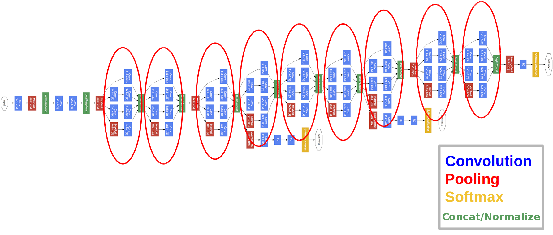
Structure of an Inception Block:
Each Inception block has multiple branches:
- 1x1 convolution
- 1x1 → 3x3 convolution
- 1x1 → 5x5 convolution
- 3x3 max pooling → 1x1 convolution
Notice how each expensive convolution is preceded by a 1x1 convolution for dimensionality reduction.
Advantages:
- Parameter Efficiency: Fewer parameters than naïvely stacking all filters.
- Rich Feature Learning: Learns features at multiple receptive fields simultaneously.
- Parallelism: More effective than deeper or wider models with uniform layers.
Example:
Assume an input of size $ 28 \times 28 \times 192 $. After passing through an Inception module, we may get something like:
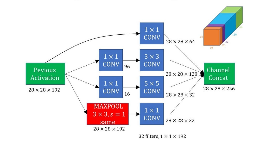
- 1x1 branch → 64 channels
- 3x3 branch → 128 channels
- 5x5 branch → 32 channels
- Pooling branch → 32 channels
- Total output depth: 256
Improvements Over Time
GoogLeNet inspired many improved versions:
- Inception v2/v3: Factorization of convolutions (e.g., 5x5 → two 3x3 layers)
- Inception v4: Combined ideas from ResNet and Inception (e.g., Inception-ResNet)
- Use of BatchNorm and Auxiliary Classifiers
These tricks improved accuracy without dramatically increasing parameters.
The Inception architecture was a major leap forward in CNN design:
- It introduced the concept of multi-path architectures
- Emphasized computational efficiency
- Leveraged 1x1 convolutions to control model complexity
This paved the way for even more efficient models like MobileNet and EfficientNet.
MobileNet and EfficientNet
MobileNet
As deep learning models became larger and deeper, they demanded more memory and computation — not ideal for mobile or embedded devices. MobileNet, introduced by Google in 2017, addressed this challenge by proposing a highly efficient architecture using depthwise separable convolutions.
Standard Convolution vs. Depthwise Separable Convolution
Let’s recall the standard convolution:
Given an input of size $ H \times W \times D_{in} $, applying $ N $ filters of size $ K \times K \times D_{in} $ produces an output of size $ H’ \times W’ \times N $.
- Computation Cost: $$ K \cdot K \cdot D_{in} \cdot N \cdot H’ \cdot W’ $$
MobileNet factorizes this into two steps:
-
Depthwise Convolution:
Apply one filter per input channel — no cross-channel combination.
Cost:$$ K \cdot K \cdot D_{in} \cdot H’ \cdot W’ $$
-
Pointwise Convolution (1x1):
Mix the depthwise output with $ N $ 1x1 filters.
Cost: $$ D_{in} \cdot N \cdot H’ \cdot W’ $$
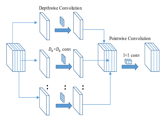
✅ Total Cost:
$$ K^2 \cdot D_{in} \cdot H’ \cdot W’ + D_{in} \cdot N \cdot H’ \cdot W’ $$
which is ~9x less than standard convolution when $ K = 3 $.
MobileNet Architecture (V1 Highlights)
MobileNetV1 is built by stacking depthwise separable convolutions instead of regular ones. It also introduces:
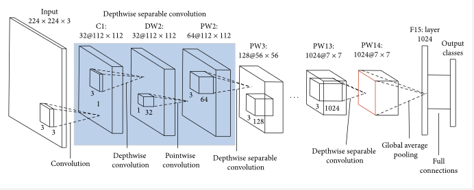
- Width Multiplier (α): Shrinks the number of channels (e.g., α=0.75 reduces model size).
- Resolution Multiplier (ρ): Reduces input image size to further save computation.
Together, these enable a trade-off between accuracy and resource usage.
MobileNet is often used as a backbone in real-time applications (e.g., object detection on smartphones, AR apps).
EfficientNet
Introduced in 2019 by Google AI, EfficientNet pushes the boundary of model performance by scaling neural networks systematically.
The Problem: How to Scale a CNN?
You can make a CNN more powerful by:
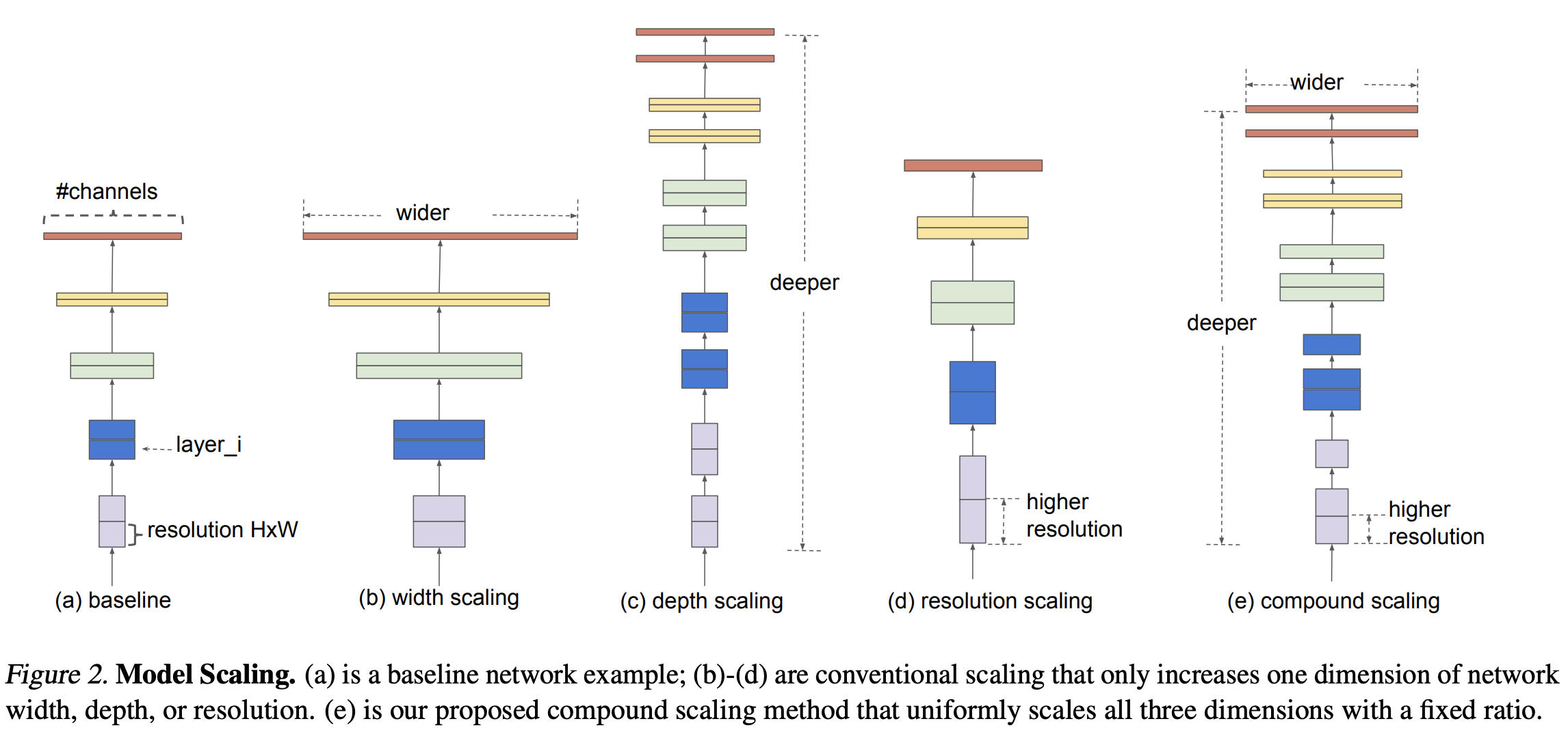
- Increasing depth (more layers)
- Increasing width (more channels)
- Increasing resolution (larger input images)
But how much of each?
Compound Scaling: Efficient Strategy
Instead of arbitrarily scaling one dimension, EfficientNet introduces a compound coefficient (ϕ) that balances all three:
$$ \begin{aligned} \text{depth:} &\quad d = \alpha^\phi \ \text{width:} &\quad w = \beta^\phi \ \text{resolution:} &\quad r = \gamma^\phi \ \text{subject to:} &\quad \alpha \cdot \beta^2 \cdot \gamma^2 \approx 2 \end{aligned} $$
- ϕ controls the available resources (e.g., more computation).
- α, β, γ are constants determined via grid search.
Performance
EfficientNet models (B0 to B7) are built on the same base architecture (EfficientNet-B0), with progressively larger values of ϕ.
- EfficientNet-B0: baseline
- EfficientNet-B1 to B7: scaled versions with increasing capacity
✅ Result:
EfficientNet achieves better accuracy with fewer parameters compared to deeper networks like ResNet-152 or Inception-v4.
| Architecture | Key Idea | Efficiency Trick |
|---|---|---|
| MobileNet | Lightweight model for mobile | Depthwise separable convolutions |
| EfficientNet | Scalable and accurate model | Compound scaling across depth, width, resolution |
Both architectures represent the evolution of CNN design towards compact, fast, and powerful models — a necessary shift for real-world AI deployment.
Object Localization and Detection
- Object Localization
- Landmark Detection
- Object Detection
- Sliding Window Approach and Its Convolutional Implementation
Object Localization
Object localization is the task of identifying the presence of an object in an image and determining its position using a bounding box.
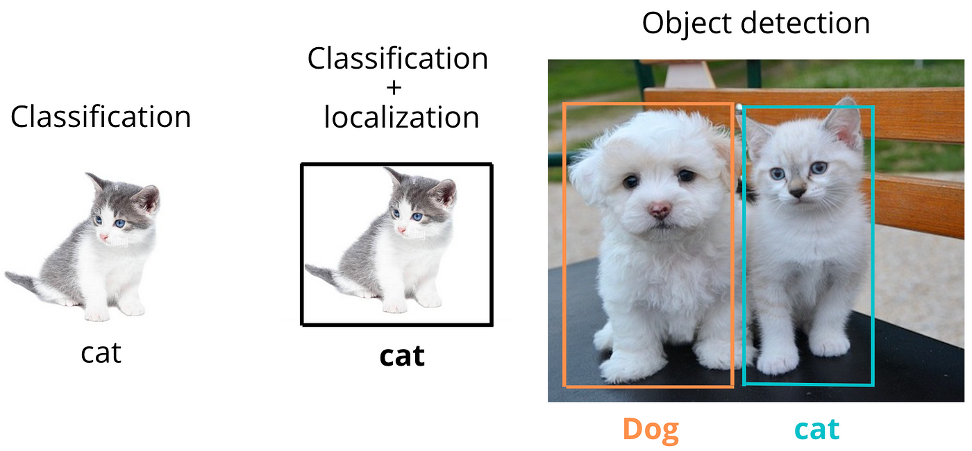
It’s one step more complex than image classification, which only tells what is in the image, not where it is.
Given an image, object localization aims to:
- Classify the object (e.g., cat, dog, car).
- Return the bounding box coordinates around the object: $$ (x_{\text{min}}, y_{\text{min}}, x_{\text{max}}, y_{\text{max}}) \quad \text{or} \quad (x, y, w, h) $$
Where:
- $ (x, y) $: center of the bounding box
- $ w, h $: width and height of the box
Output Vector
If you’re using a neural network for localization, the output vector might be:
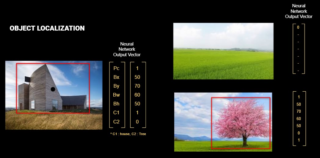
$$ \text{Output} = [p_c, x, y, w, h, c_1, c_2, …, c_n] $$
Where:
- $ p_c $: Probability that an object exists in the image
- $ x, y, w, h $: Bounding box
- $ c_i $: Class probabilities (e.g., cat = 0.8, dog = 0.2)
If the object whose class is defined cannot be detected on the image, $p_c$ will be $0$. In the case where $p_c$ is $0$, the bounding box values ($x ,y, w, h$) and class values are insignificant in the vector. This means that they are not included when calculating the Loss function.
Loss Function
A multi-part loss is generally used for localization:
- Localization loss (coordinate regression): Measures error in predicted box location
- Confidence loss (objectness): Measures error in object existence
- Classification loss: Measures class prediction error
Example (simplified version as in YOLO):
$$ \mathcal{L} = \lambda_{\text{coord}} \cdot \sum_{i} \mathbb{1}_{i}^{\text{obj}} \left[(x_i - \hat{x}_i)^2 + (y_i - \hat{y}_i)^2 + (w_i - \hat{w}_i)^2 + (h_i - \hat{h}_i)^2\right] + \text{classification loss} $$
Landmark Detection
Landmark detection (also called keypoint detection) involves detecting specific key locations on an object. Unlike bounding boxes, keypoints give finer-grained localization.
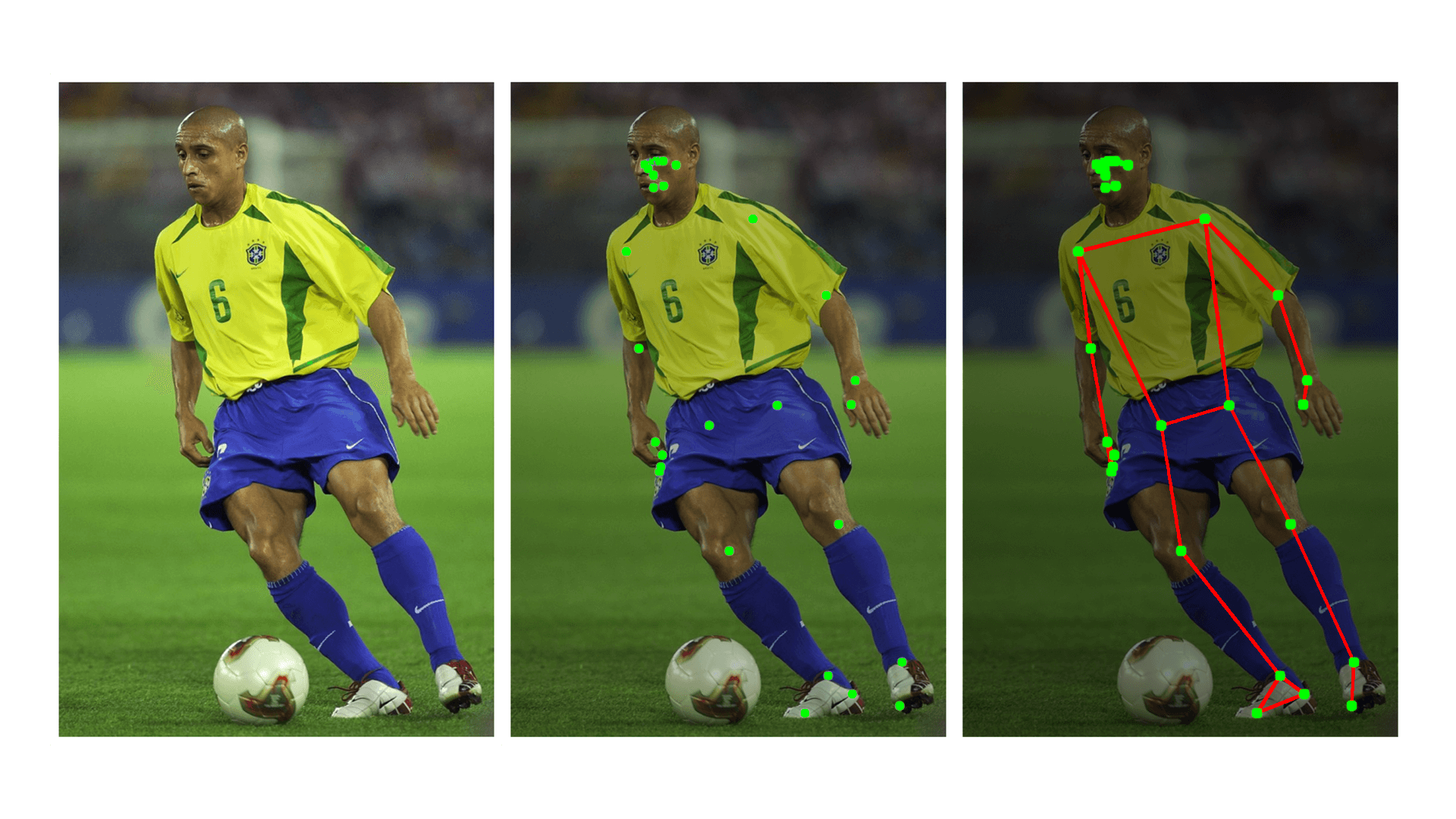
Example
- Face recognition: Eyes, nose tip, mouth corners
- Hand detection: Fingertips and joints
- Medical imaging: Identifying organ boundaries
Output Representation
If we detect $ K $ landmarks:
$$ \text{Output} = [x_1, y_1, x_2, y_2, …, x_K, y_K] $$
Each pair represents the $(x, y)$ coordinate of a keypoint like knee point or ear point.
Loss Function
The typical loss for landmark detection:
$$ \mathcal{L}{\text{keypoints}} = \sum{k=1}^{K} \left[(x_k - \hat{x}_k)^2 + (y_k - \hat{y}_k)^2\right] $$
Object Detection
Object detection combines classification and localization — but now for multiple objects in the same image.
Example
In a single street photo:
- Detect a car (class = car, bounding box)
- Detect a pedestrian (class = human, bounding box)
- Detect a stop sign (class = sign, bounding box)
Compared to Localization
| Task | Output |
|---|---|
| Classification | Class label |
| Localization | Class + bounding box |
| Detection | Multiple classes + boxes |
Model Output Structure
We divide the image into an $ S \times S $ grid. For each grid cell, predict:
- $ B $ bounding boxes
- Confidence score
- Class probabilities
$$ \text{Output Tensor} = S \times S \times (B \cdot 5 + C) $$
Where:
- Each box includes $[p_c, x, y, w, h]$. $5$ means this vector.
- $ C $: number of classes
Sliding Window Approach and Its Convolutional Implementation
The sliding window technique is a classic method in computer vision used for object detection. The core idea is to take a fixed-size rectangular window and slide it across the input image, systematically checking each region to see whether it contains the object of interest.
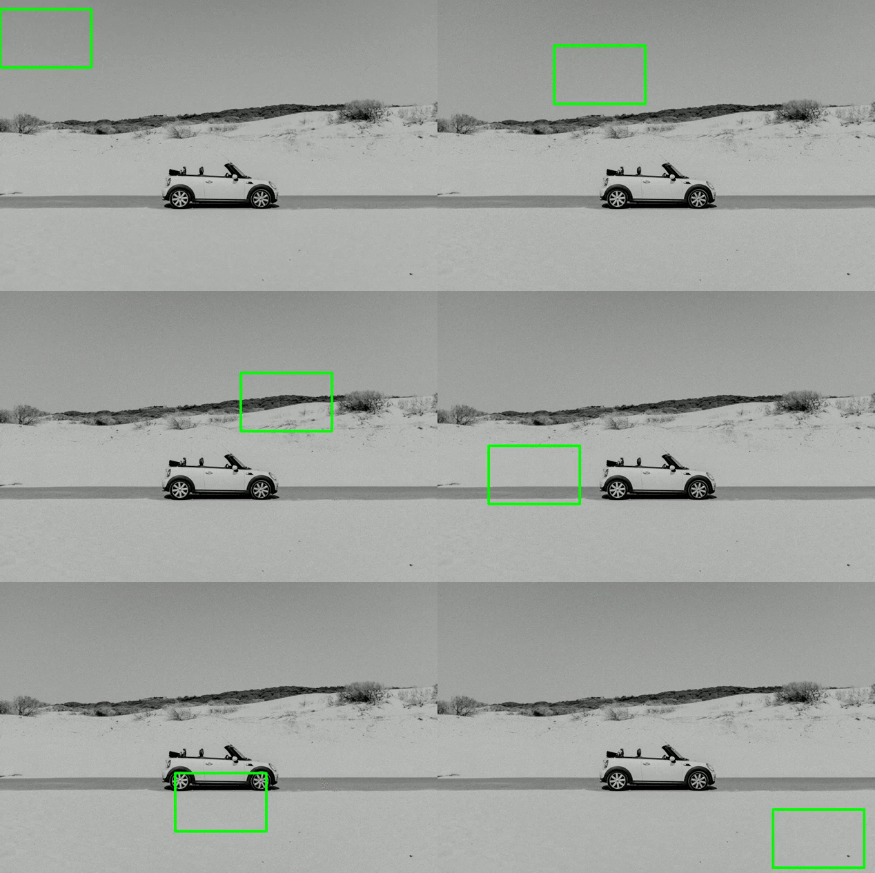
At each window position, the cropped image region is passed to a classifier (e.g., SVM, logistic regression, or a small CNN) to determine whether it contains an object. This window “slides” over the image both horizontally and vertically, often with some stride value, producing many cropped regions.
It converts a classification model into a localization tool by brute-force scanning over all possible positions.
Limitations of Naive Sliding Windows
Although conceptually simple, the naive sliding window method has serious drawbacks:
1. High Computational Cost
- For an image of size $ W \times H $, using a window of size $ w \times h $ with stride $ s $, the number of windows is: $$ \left(\frac{W - w}{s} + 1\right) \cdot \left(\frac{H - h}{s} + 1\right) $$ This can result in thousands of regions even for medium-sized images.
- Each window requires a separate forward pass through the classifier network, resulting in massive redundancy since overlapping windows share most of their pixels.
2. Difficulty in Handling Multiple Scales
- Objects in an image can appear at different scales and aspect ratios.
- To address this, either the image must be resized many times or the window size must vary — both of which further increase computation.
3. Fixed Window Shape
- Sliding windows generally use a fixed aspect ratio and size, which makes them less effective for detecting objects with irregular shapes.
Convolutional Implementation of Sliding Windows
To overcome these inefficiencies, modern approaches use the convolutional structure of neural networks to implement the sliding window more efficiently.
Key Insight: Convolutions as Shared Computation
Instead of running the classifier separately on each window, we can:
- Pass the entire image through the convolutional layers of a CNN once
- These layers produce a feature map where each spatial position encodes information about a local receptive field (i.e., a subregion of the image)
- This naturally simulates a sliding window operation
Then, we apply 1x1 convolutions or fully connected layers converted into convolutions over the feature map to produce dense predictions for object presence.
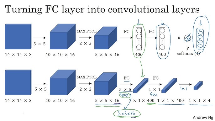
Fully Connected Layer to Convolution
A fully connected layer expecting a flattened $ N \times N \times D $ input can be rewritten as a 1x1 convolution over a $ N \times N \times D $ feature map:
- Each position in the resulting output map corresponds to a specific receptive field on the original image
- This effectively implements classification over many regions at once, reusing shared computation
Use in Modern Architectures
Understanding the YOLO (You Only Look Once) Architecture
YOLO (You Only Look Once) is a real-time object detection system that reframes object detection as a single regression problem, rather than a classification or region proposal problem. Instead of scanning the image multiple times or generating multiple proposals, YOLO sees the entire image only once and directly outputs bounding boxes and class probabilities in a single evaluation.
This end-to-end architecture enables extremely fast inference and is designed for real-time applications such as self-driving cars, robotics, surveillance, and augmented reality.
How Does YOLO Work?
At a high level, YOLO divides the input image into a fixed-size grid and makes predictions for each grid cell. Let’s go through each part of the architecture:
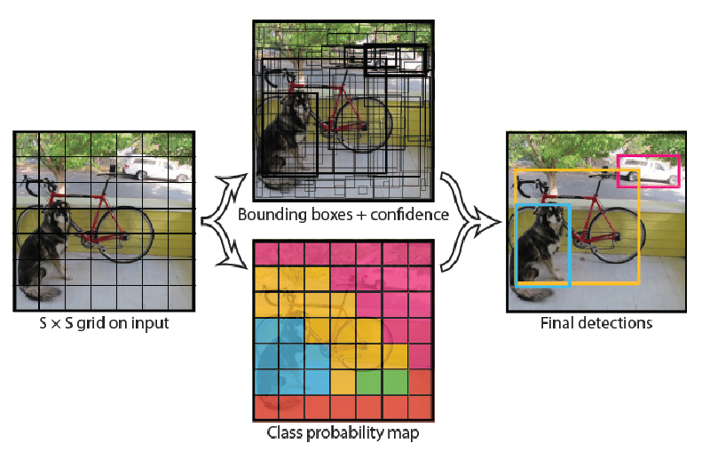
1. Image Grid Division
- The input image is divided into an $ S \times S $ grid (e.g., $ 7 \times 7 $).
- Each grid cell is responsible for detecting objects whose center falls inside the cell.
2. Bounding Box Predictions
Each grid cell predicts:
- $ B $ bounding boxes (typically $ B = 2 $)
- For each box:
- $ x, y $: coordinates of the box center (relative to the grid cell)
- $ w, h $: width and height of the box (relative to the whole image)
- $ p_c $: confidence score = $ P(\text{object}) \times \text{IoU} {\text{pred,truth}} $
3. Class Probabilities
-
Each grid cell also predicts $ C $ conditional class probabilities:
$$ P(\text{class}_i \mid \text{object}) \quad \text{for } i = 1, \dots, C $$
-
These probabilities are class probabilities conditioned on the presence of an object in the cell.
4. Final Predictions
- The total output per grid cell is: $$ B \times [p_c, x, y, w, h] + C $$ For example, with $ S = 7 $, $ B = 2 $, $ C = 20 $, the total prediction tensor size is: $$ 7 \times 7 \times (2 \times 5 + 20) = 7 \times 7 \times 30 $$
Why Is It Called “You Only Look Once”?
Traditional detection pipelines involve:
- Generating region proposals (like in R-CNN)
- Running a CNN on each region
- Performing classification and box regression separately
YOLO unifies this pipeline into a single CNN pass, hence the name “You Only Look Once”. The model sees the full image context and outputs all bounding boxes and class scores in one go.
SSD (Single Shot MultiBox Detector)
- Detects objects at multiple scales using feature maps from different layers
- Uses convolutional layers to predict class and box offsets at every location in the feature map
Summary
| Approach | Characteristics |
|---|---|
| Naive Sliding Window | Slow, inefficient, redundant computation |
| Convolutional Sliding | Efficient, shared computation, suitable for real-time detection |
By understanding this transition from brute-force scanning to convolutional prediction, we appreciate how convolutional networks not only recognize what is in an image but also where, enabling scalable object detection.
Evaluation and Optimization: IoU, Non-max Suppression, Anchor Boxes
Intersection over Union (IoU)
Intersection over Union (IoU) is a metric used to evaluate the accuracy of an object detector on a particular dataset. It measures the overlap between two bounding boxes:
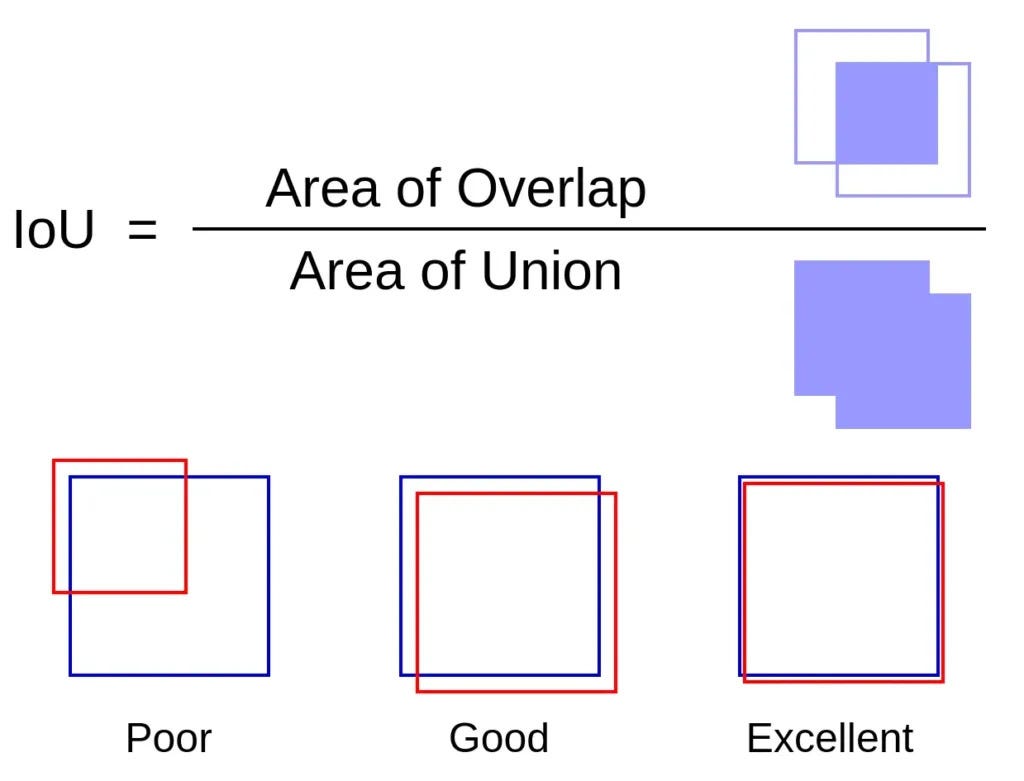
- The predicted bounding box
- The ground-truth bounding box
Mathematical Definition
If $B_p$ is the predicted bounding box and $B_{gt}$ is the ground truth bounding box:
$$ IoU = \frac{Area(B_p \cap B_{gt})}{Area(B_p \cup B_{gt})} $$
- $IoU = 1.0$: perfect overlap
- $IoU = 0.0$: no overlap
Example
Suppose:
- Predicted box: top-left = (50, 50), bottom-right = (150, 150)
- Ground truth: top-left = (100, 100), bottom-right = (200, 200)
The overlapping area is a square from (100, 100) to (150, 150) → 50x50 = 2500
Total area:
- Predicted: $100 \times 100 = 10,000$
- GT: $100 \times 100 = 10,000$
- Union: $10,000 + 10,000 - 2,500 = 17,500$
So,
$$ IoU = \frac{2500}{17500} = 0.143 $$
Use in Training and Evaluation
- In training, you may ignore detections with IoU < 0.5
- For evaluation, mAP (mean average precision) uses IoU thresholds (e.g., 0.5 or 0.75)
Non-max Suppression (NMS)
Why Do We Need It?
Object detectors often output multiple overlapping boxes for a single object. NMS filters out redundant boxes by keeping the one with the highest confidence score.
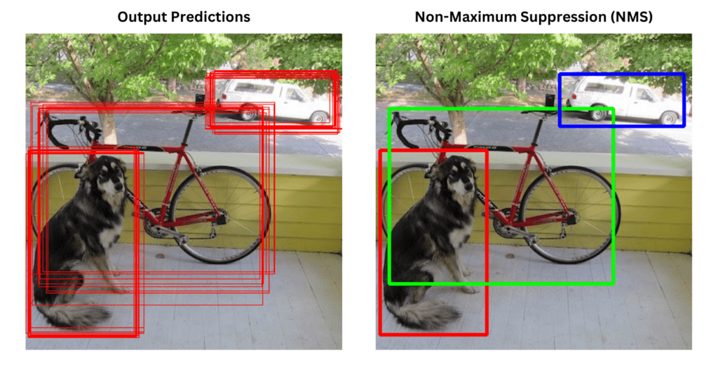
Algorithm Steps
- Sort all bounding boxes by their confidence score.
- Select the box with the highest confidence and remove it from the list.
- Compute IoU between this box and all others.
- Remove boxes with IoU above a threshold (e.g., 0.5).
- Repeat until no boxes remain.
Mathematical Intuition
Let $B_i$ be a box with score $s_i$. You iterate over all boxes and apply:
$$ \text{Keep } B_i \text{ if } IoU(B_i, B_j) < T, \forall j < i $$
Where $T$ is the suppression threshold.
Anchor Boxes
What are Anchor Boxes?
Anchor boxes (also called prior boxes) are predefined bounding boxes with different shapes and sizes. They allow object detectors to:
- Detect multiple objects in the same grid cell
- Handle aspect ratio and scale variation
Why Are They Needed?
Without anchor boxes, a single grid cell could detect only one object. But real-world scenes often contain overlapping or closely spaced objects.
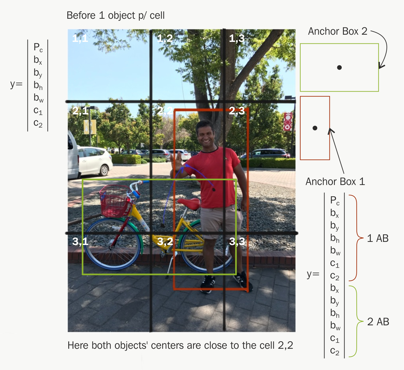
Anchor Box Design
You predefine $k$ anchor boxes per cell. Each one is defined by:
- Width $w$
- Height $h$
- Aspect ratio $r = \frac{w}{h}$
For example, in SSD:
- 3 feature maps
- 6 anchors per feature cell
- $\Rightarrow$ 8732 total anchor boxes
Output Format with Anchors
For each anchor box, the network predicts:
- $\Delta x, \Delta y$: offset from anchor center
- $\Delta w, \Delta h$: log scale changes to width and height
- Confidence score
- Class probabilities
This transforms anchor box $(x_a, y_a, w_a, h_a)$ to the predicted box $(x_p, y_p, w_p, h_p)$:
$$ x_p = x_a + w_a \cdot \Delta x \ y_p = y_a + h_a \cdot \Delta y \ w_p = w_a \cdot e^{\Delta w} \ h_p = h_a \cdot e^{\Delta h} $$
Summary
- IoU measures overlap and is used for loss/evaluation.
- Non-max suppression removes redundant boxes based on IoU.
- Anchor boxes allow detection of multiple objects at different scales/aspect ratios.
Together, these techniques form the foundation of modern object detection pipelines like YOLO, SSD, and Faster R-CNN.
Region Proposals and Semantic Segmentation: U-Net
- Region Proposals
- Semantic Segmentation
- Transpose Convolutions (Deconvolution)
- U-Net Architecture Intuition
- U-Net Architecture (Full Design)
- Summary
Region Proposals
Why Region Proposals?
Traditional object detectors like sliding windows are computationally expensive due to scanning every possible region in the image. Region Proposal methods address this by generating a small number of candidate regions likely to contain objects.
Selective Search
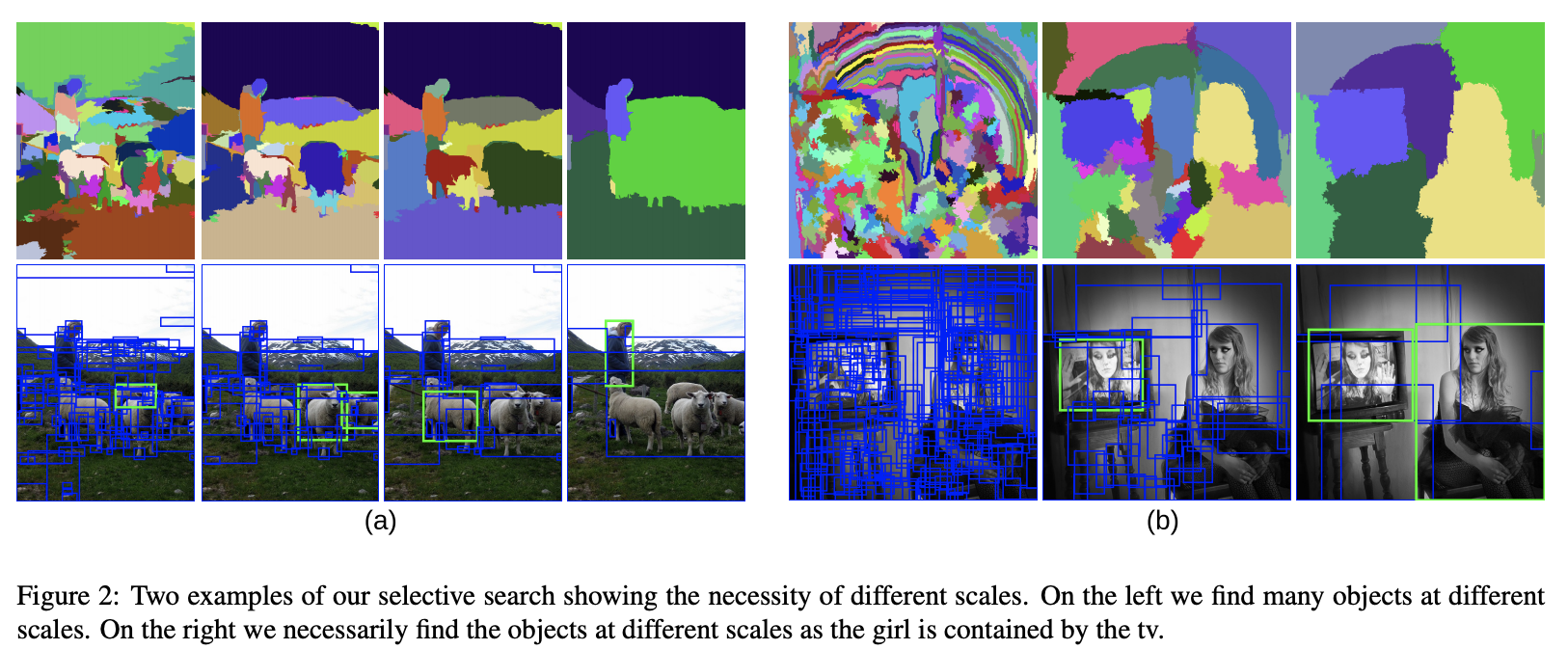
- Group similar pixels into superpixels
- Merge regions based on similarity
- Outputs ~2000 proposals per image
R-CNN Pipeline
- Use Selective Search to propose regions.
- Warp each region to a fixed size (e.g., 224x224).
- Pass through a ConvNet to extract features.
- Use SVMs for classification and regressors for bounding boxes.
Limitation: Very slow due to independent ConvNet run on each region.
Semantic Segmentation
What is Semantic Segmentation?
Semantic segmentation is the task of classifying each pixel of an image into a class label.
- Image Classification: What is in the image?
- Object Detection: Where is the object?
- Semantic Segmentation: Which pixel belongs to which class?
Applications
- Medical imaging (e.g., tumor segmentation)
- Autonomous driving (lane and pedestrian detection)
- Satellite image analysis
- Industrial defect detection
Transpose Convolutions (Deconvolution)
Motivation
In segmentation tasks, we need to upsample feature maps back to the original image size. Transpose convolutions (a.k.a. deconvolutions) help with this.
How It Works
A transpose convolution is the reverse of a normal convolution:
- While convolution reduces spatial size (downsampling),
- Transpose convolution increases it (upsampling).
Mathematical Operation
Suppose an input size of $N \times N$ and a kernel size of $k \times k$ with stride $s$.
-
Convolution output size:
$$ O = \left\lfloor \frac{N - k}{s} + 1 \right\rfloor $$
-
Transpose convolution (reverses the above): $$ O_{up} = (N - 1) \cdot s + k $$
Alternatives
- Nearest-neighbor or bilinear upsampling + 1x1 conv (cheaper, less expressive)
- Learned transpose convolutions (richer)
U-Net Architecture Intuition
Key Idea
U-Net is a fully convolutional network that consists of:
- A contracting path to capture context (downsampling)
- An expanding path to enable precise localization (upsampling)
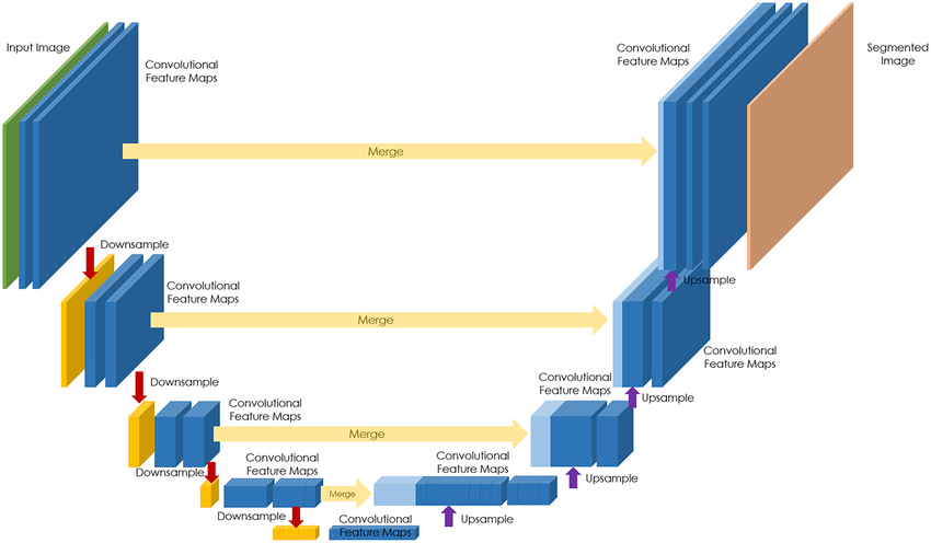
U-Net was originally designed for biomedical image segmentation but is now used in many fields.
Contracting Path (Encoder)
- Similar to standard CNN (e.g., VGG)
- Repeated 2x:
- Conv (ReLU) → Conv (ReLU) → MaxPooling
Expanding Path (Decoder)
- Transpose convolution for upsampling
- Skip connections concatenate features from encoder
Why Skip Connections?
Skip connections pass high-resolution features from encoder to decoder, enabling:
- Better boundary localization
- Preservation of fine details
U-Net Architecture (Full Design)
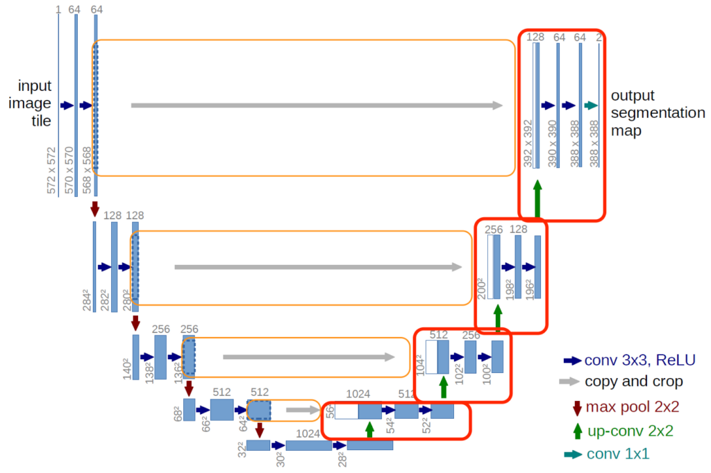
Structure Overview
- Input size: $572 \times 572$
- Each layer: two $3 \times 3$ convolutions + ReLU
- Downsampling: $2 \times 2$ max-pooling
- Upsampling: transpose convolutions
- Final output: $1 \times 1$ convolution to map to $C$ classes (per pixel)
Example Architecture
Input → Conv → Conv → Pool
↓ ↑
Conv → Conv → Pool
↓ ↑
Conv → Conv → Pool
↓ ↑
Bottleneck ← Skip Connections
↓ ↑
Upconv → Concat → Conv → Conv
↓
Output (Segmentation Map)
Loss Function
Typical loss: Pixel-wise cross-entropy loss.
$$ \mathcal{L} = - \sum_{i=1}^{H} \sum_{j=1}^{W} \sum_{c=1}^{C} y_{ij}^{(c)} \log(\hat{y}_{ij}^{(c)}) $$
Where:
- $H, W$: height and width of the image
- $C$: number of classes
- $y_{ij}^{(c)}$: ground truth indicator (1 if pixel $(i,j)$ belongs to class $c$)
- $\hat{y}_{ij}^{(c)}$: predicted probability for class $c$ at pixel $(i,j)$
Performance Metrics
- Pixel Accuracy: overall correct classification
- IoU per class: same as object detection, applied per-pixel
- Dice Coefficient: common in medical segmentation
Summary
- Region proposals are key to efficient object detection pipelines like R-CNN.
- Semantic segmentation classifies each pixel and requires upsampling layers.
- Transpose convolutions allow learned upsampling.
- U-Net combines low-level and high-level features through skip connections and is state-of-the-art for many segmentation tasks.
Face Recognition and Neural Style Transfer
What is Face Recognition?
Face recognition is the task of identifying or verifying a person’s identity using their facial features. It can be broken down into three main categories:
- Face Detection: Locate faces in an image (bounding box).
- Face Verification: Check if two faces are of the same person (1:1 comparison).
- Face Recognition/Identification: Identify a person from a database (1:N comparison).
Real-World Applications
- Smartphone unlock (Face ID)
- Security surveillance
- Online proctoring
- Social media tagging (e.g., Facebook)
One Shot Learning
Traditional classification algorithms require many training examples per class. However, in face recognition:
- We might only have one image per person.
- The task becomes: Can the model recognize a face it has seen only once?
This is known as One-Shot Learning.
Problem Setup
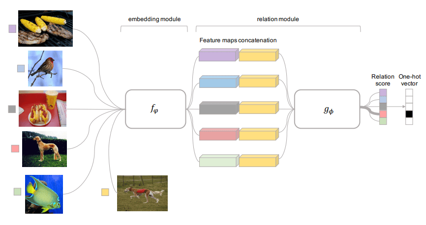
- Instead of learning to classify, the model learns similarity between pairs of images.
- A distance function is trained to return a small value for the same person, and large for different people.
Siamese Network
A Siamese Network consists of two identical ConvNets (with shared weights) that compare two inputs.
Architecture Overview
- Two inputs: $x_1$ and $x_2$
- Same CNN maps both to feature vectors $f(x_1)$ and $f(x_2)$
- A distance metric (e.g., L2 norm) is applied:
$$ d(x_1, x_2) = |f(x_1) - f(x_2)|_2^2 $$
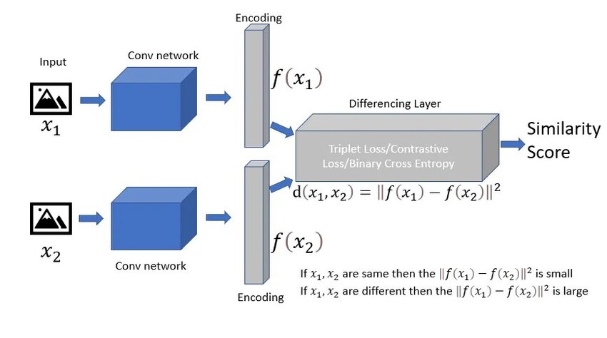
Loss Function
A contrastive loss or triplet loss is used to train the network to minimize distances for same identities and maximize for different ones.
Triplet Loss
Triplet Loss is a powerful loss function for learning embeddings. It relies on triplets:
- Anchor (A): A known image
- Positive (P): Image of the same identity
- Negative (N): Image of a different identity
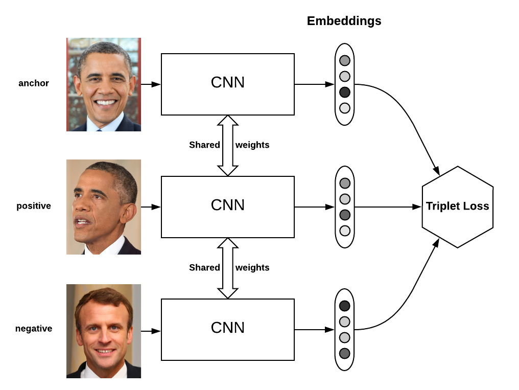
We want:
$$ |f(A) - f(P)|_2^2 + \alpha < |f(A) - f(N)|_2^2 $$
Where:
- $f(x)$ is the embedding function (ConvNet output)
- $\alpha$ is a margin to separate positive and negative pairs
Loss Function
The Triplet Loss is:
$$ \mathcal{L}(A, P, N) = \max\left(|f(A) - f(P)|_2^2 - |f(A) - f(N)|_2^2 + \alpha, 0\right) $$
Important Notes
- Semi-hard negative mining improves convergence (choose negatives that are hard but not too hard).
- Embeddings are often normalized to unit length.
Face Verification and Binary Classification
Once we have embeddings from a trained network (e.g., using triplet loss), we can perform face verification as a binary classification task.
Verification Pipeline
- Encode both face images to embeddings.
- Compute Euclidean distance or cosine similarity.
- If distance < threshold $\Rightarrow$ same person.
Threshold $\theta$ is selected based on False Positive Rate vs. True Positive Rate using ROC curve on a validation set.
What is Neural Style Transfer?
Neural Style Transfer is the task of synthesizing an image that:
- Preserves the content of a content image
- Adopts the style of a style image
Leverage a pre-trained ConvNet (like VGG19) to extract content and style representations.
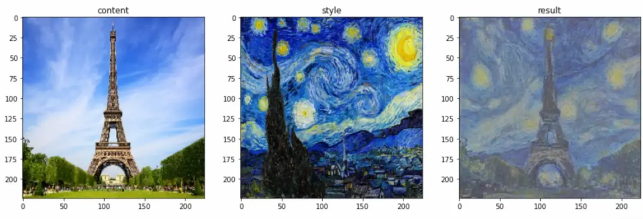
Let:
- $C$ be the content image
- $S$ be the style image
- $G$ be the generated image
Then we optimize $G$ to minimize a cost function:
$$ J(G) = \alpha J_{content}(C, G) + \beta J_{style}(S, G) $$
What are Deep ConvNets Learning?
Deep ConvNets learn hierarchical representations:

- Early layers: edges, colors, textures
- Mid layers: shapes, motifs
- Later layers: object-level concepts
In NST, content is encoded in deeper layers, style in shallower layers.
Cost Function
The total cost is:
$$ J(G) = \alpha J_{content}(C, G) + \beta J_{style}(S, G) $$
Where:
- $\alpha$: weight for content preservation
- $\beta$: weight for style transfer
- Typically: $\alpha = 1$, $\beta = 10^3$ to $10^4$
Content Cost Function
Let $a^{l}$ and $a^{l}$ be activations at layer $l$ for the content and generated images.
Then content cost is:
$$ J_{content}(C, G) = \frac{1}{2} |a^{l} - a^{l}|_2^2 $$
Use a deeper layer (e.g., conv4_2) for this.
Style Cost Function
Style is captured by correlations between feature maps using a Gram matrix.
Let $a^{l}$ be the activations at layer $l$ for style image. Compute Gram matrix:
$$ G_{ij}^{[l]} = \sum_k a_{ik}^{[l]} a_{jk}^{[l]} $$
Style cost is:
$$ J_{style}^{[l]}(S, G) = \frac{1}{(2n_H n_W n_C)^2} |G^{l} - G^{l}|_F^2 $$
Then sum over multiple layers:
$$ J_{style}(S, G) = \sum_l \lambda^{[l]} J_{style}^{[l]}(S, G) $$
1D and 3D Generalizations
1D Generalization
Neural style transfer principles can be applied to audio signals:
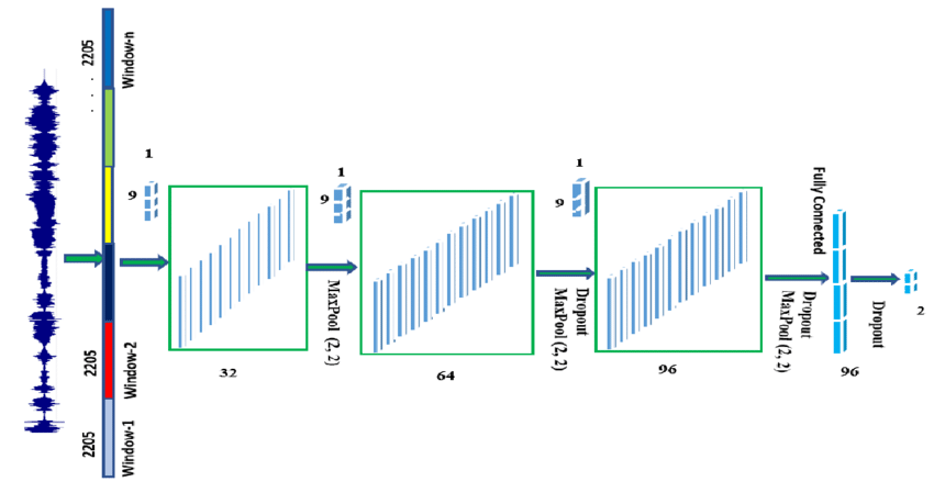
- 1D convolution over waveform
- Preserve temporal content, apply style of another sound
3D Generalization
Applied to volumetric data such as:
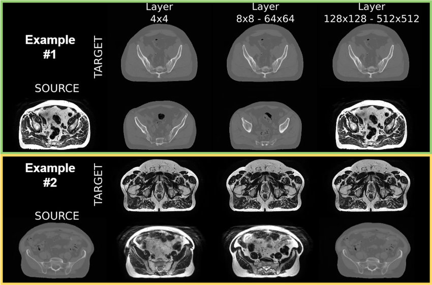
- 3D MRI scans
- 3D point clouds
- Transfer spatial styles across 3D volumes
These require 3D convolutional layers and custom Gram matrix calculations.
Summary
- Face Recognition uses embedding learning (Triplet loss, Siamese networks).
- One-shot learning enables models to generalize with limited data.
- Neural Style Transfer uses a pre-trained CNN to blend content and style images using a combination of content/style loss.
- Both applications showcase the expressive power of deep convolutional networks beyond classic classification.
Recurrent Neural Networks (RNNs)
- Why Sequence Models?
- Notation
- Recurrent Neural Network Model
- Backpropagation Through Time
- Different Types of RNNs
- Language Model and Sequence Generation
- Sampling Novel Sequences
- Vanishing Gradients with RNNs
- Gated Recurrent Unit (GRU)
- Long Short-Term Memory (LSTM)
- Bidirectional RNN
- Deep RNNs
Why Sequence Models?
Sequence models are used when the input and/or output is sequential. For example:
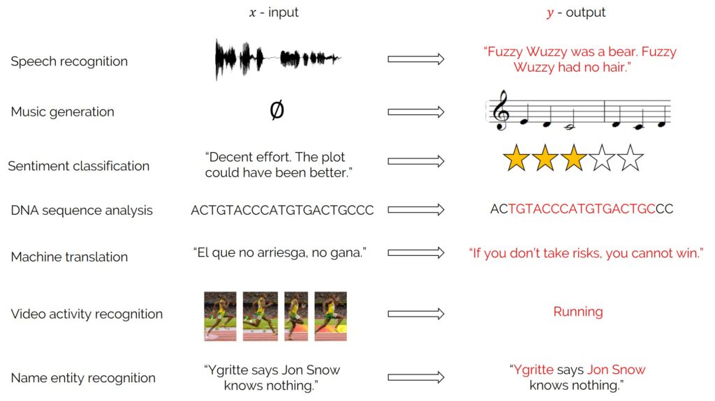
They model dependencies over time or sequence positions, which standard feedforward neural networks cannot do efficiently.
Notation
- $x^{(t)}$: input at time step $t$
- $y^{(t)}$: output at time step $t$
- $a^{(t)}$: hidden state at time step $t$
- $\hat{y}^{(t)}$: predicted output at time step $t$
- $T$: sequence length
Recurrent Neural Network Model
The RNN computes:
- $a^{(t)} = anh(W_{aa}a^{(t-1)} + W_{ax}x^{(t)} + b_a)$
- $\hat{y}^{(t)} = ext{softmax}(W_{ya}a^{(t)} + b_y)$
RNNs share parameters across time, allowing generalization to different sequence lengths.
Backpropagation Through Time
To train RNNs, we use backpropagation through time (BPTT):
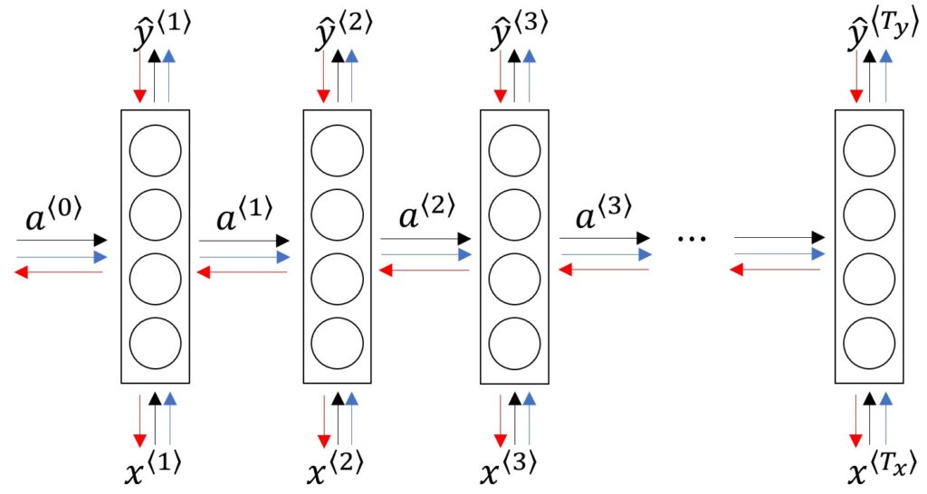
- Unroll the RNN for $T$ steps
- Compute loss and gradients across all time steps
- Apply chain rule for gradients through time dependencies
Different Types of RNNs
- Many-to-Many: sequence input and sequence output (e.g., machine translation)
- Many-to-One: sequence input, single output (e.g., sentiment analysis)
- One-to-Many: single input, sequence output (e.g., image captioning)
Language Model and Sequence Generation
Language models predict the next word given a sequence:
- $P(y^{(t)} | y^{(1)}, …, y^{(t-1)})$
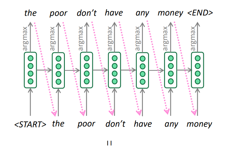
Training: minimize cross-entropy loss between predicted and actual next words.
Sampling Novel Sequences
- Start with a seed (e.g.,
) - Sample $y^{(1)}$, feed it back
- Continue until
or max length
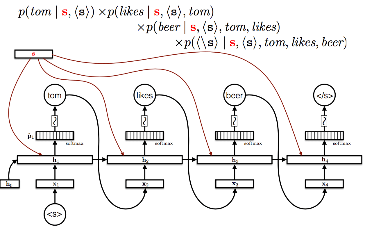
Sampling temperature can control randomness:
- Low temperature = conservative (likely choices)
- High temperature = creative (diverse outputs)
Vanishing Gradients with RNNs
One of the fundamental challenges in training RNNs is the vanishing gradient problem, especially when modeling long-term dependencies.
When computing gradients using Backpropagation Through Time (BPTT), the gradients at earlier time steps are affected by the repeated multiplication of small values (from derivatives of activation functions like tanh or sigmoid). This leads to:
- Gradients becoming very small (vanish): weights are barely updated for earlier time steps
- Gradients becoming very large (explode): instability and divergence in training
Intuition with Example:
Consider a sequence: “I grew up in France… I speak fluent ___”
The model needs to learn that the word “French” depends on the context word “France” seen many time steps earlier. If the gradient shrinks too much over those steps, the model fails to learn this dependency.
Consequences:
- Short-term dependencies are learned effectively.
- Long-term dependencies are often lost.
Gated Recurrent Unit (GRU)
Why do we need GRUs?
Traditional RNNs struggle with learning long-term dependencies due to the vanishing gradient problem. As sequences grow longer, the gradients used during backpropagation either shrink or explode, making it hard for the network to retain information over time.
GRUs are designed to solve this by introducing gating mechanisms that control what information should be remembered, updated, or forgotten. These gates make the network more efficient at learning dependencies in long sequences.
GRU introduces gates to control information flow:
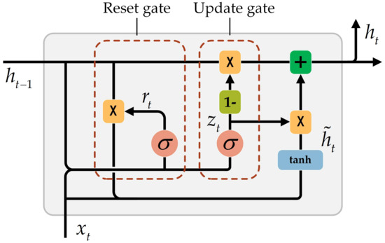
A GRU has two main gates:
-
Update Gate ($z$):
-
Determines how much of the previous memory to keep.
-
If z ≈ 1, it keeps the old memory.
-
If z ≈ 0, it updates with new information.
-
-
Reset Gate ($r$):
-
Controls how much of the previous state should be ignored.
-
Helps in deciding whether to forget the old state when generating the new memory.
-
Equations:
- $z^{(t)} = \sigma(W_zx^{(t)} + U_za^{(t-1)} + b_z)$
- $r^{(t)} = \sigma(W_rx^{(t)} + U_ra^{(t-1)} + b_r)$
- $\tilde{a}^{(t)} = \tanh(Wx^{(t)} + U(r^{(t)} \ast a^{(t-1)}) + b)$
- $a^{(t)} = (1 - z^{(t)}) * a^{(t-1)} + z^{(t)} * \tilde{a}^{(t)}$
GRU vs Traditional RNN
| Feature | RNN | GRU |
|---|---|---|
| Memory control | None | Yes (update/reset gates) |
| Vanishing gradients | Common | Less frequent |
| Parameter efficiency | Fewer params | More, but fewer than LSTM |
| Training speed | Fast | Slower than RNN, faster than LSTM |
Example: Sequence with Context
Imagine trying to classify the sentiment of the sentence:
“The movie was terrible… but the ending was amazing.”
- A vanilla RNN might forget the earlier “terrible” and overly weight the “amazing”, resulting in an incorrect positive classification.
- A GRU, however, can learn to retain both sentiments and give a more balanced representation by preserving long-term context.
Long Short-Term Memory (LSTM)
Why Do We Need LSTM?
Traditional RNNs struggle with long-term dependencies due to vanishing gradients, which hinder learning over long sequences.
To solve this, LSTMs introduce memory cells and gates that help preserve and regulate information across time steps.
LSTM Architecture Intuition
LSTM cells introduce three gates to control information:
- Forget Gate: Decides what information to throw away from the cell state.
- Input Gate: Decides which new information should be stored in the cell state.
- Output Gate: Decides what to output based on the cell state.
This gating mechanism allows the model to retain relevant information over long durations while discarding unnecessary data.
LSTM Cell: Step-by-Step
Let’s break down an LSTM cell computation for a single time step $ t $. Let:
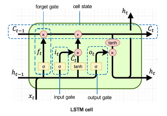
- $ x^{\langle t \rangle} $: input at time $ t $
- $ a^{\langle t-1 \rangle} $: hidden state from previous step
- $ c^{\langle t-1 \rangle} $: cell state from previous step
Then, the LSTM performs the following operations:
-
Forget Gate $ f^{\langle t \rangle} $:
$$ f^{\langle t \rangle} = \sigma(W_f \cdot [a^{\langle t-1 \rangle}, x^{\langle t \rangle}] + b_f) $$
Decides what to forget from the previous cell state.
-
Input Gate $ i^{\langle t \rangle} $ and Candidate Values $ \tilde{c}^{\langle t \rangle} $:
$$ i^{\langle t \rangle} = \sigma(W_i \cdot [a^{\langle t-1 \rangle}, x^{\langle t \rangle}] + b_i) $$
$$ \tilde{c}^{\langle t \rangle} = \tanh(W_c \cdot [a^{\langle t-1 \rangle}, x^{\langle t \rangle}] + b_c) $$
Determines what new information to add to the cell state.
-
Update Cell State:
$$ c^{\langle t \rangle} = f^{\langle t \rangle} - c^{\langle t-1 \rangle} + i^{\langle t \rangle} - \tilde{c}^{\langle t \rangle} $$
-
Output Gate $ o^{\langle t \rangle} $ and Hidden State $ a^{\langle t \rangle} $: $$ o^{\langle t \rangle} = \sigma(W_o \cdot [a^{\langle t-1 \rangle}, x^{\langle t \rangle}] + b_o) $$ $$ a^{\langle t \rangle} = o^{\langle t \rangle} * \tanh(c^{\langle t \rangle}) $$
Example: Comparing RNN and LSTM
Suppose we want to predict the next word in a sentence. Let’s compare:
RNN:
- Struggles to maintain context when sentences are long.
- For example:
"The cat, which was chased by the dog, ran up the..." → "tree"→ the subject “cat” may be forgotten.
LSTM:
- Maintains the context of “the cat” and successfully predicts
"tree".
| Feature | RNN | LSTM |
|---|---|---|
| Handles Long-Term Dependencies | ❌ | ✅ |
| Vanishing Gradient Resistant | ❌ | ✅ |
| Uses Gates | ❌ | ✅ (Forget, Input, Output) |
| Computational Complexity | Low | Higher, but more expressive |
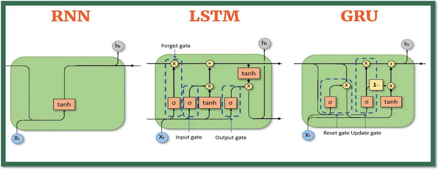
LSTMs are widely used in natural language processing, speech recognition, time series forecasting, and anywhere long-term memory is crucial.
Bidirectional RNN
In a standard RNN, information flows in a single direction — typically from past to future. However, in many tasks (like speech recognition or named entity recognition), context from both past and future words is useful for understanding the current input. This is where Bidirectional RNNs (BiRNNs) come in.
Why Use Bidirectional RNNs?
A Bidirectional RNN processes the input sequence in both directions with two separate hidden layers:
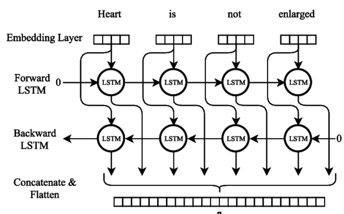
- One moves forward through time (from $x_1$ to $x_T$)
- One moves backward through time (from $x_T$ to $x_1$)
The outputs of both directions are concatenated at each time step:
$$ \overrightarrow{h}^{(t)} = \text{forward RNN output at time } t \ \overleftarrow{h}^{(t)} = \text{backward RNN output at time } t \ h^{(t)} = [\overrightarrow{h}^{(t)}; \overleftarrow{h}^{(t)}] $$
- Access to future context: Helps the model make better predictions at each time step.
- Improved performance: Especially effective in tasks where the meaning of a word depends on both previous and next words.
Imagine the sentence:
“He said he saw a bat.”
If we only process the sentence from left to right, the meaning of the word “bat” is unclear until we see the following context. A Bidirectional RNN can process both directions and better disambiguate the meaning using the full sentence context.
Applications
- Named Entity Recognition (NER)
- Part-of-Speech (POS) tagging
- Speech recognition
- Text classification
Bidirectional RNNs are often used with LSTM or GRU units to capture long-term dependencies more effectively in both directions.
Deep RNNs
Deep RNNs consist of stacking multiple recurrent layers on top of each other, allowing the network to learn hierarchical representations of sequences. By increasing the depth, the model can capture more complex temporal patterns and abstractions.
- Each layer’s output serves as input to the next recurrent layer.
- Enables learning of higher-level features across time steps.
- Can improve model capacity and expressiveness.
Challenges:
- Increased risk of overfitting due to more parameters.
- Training can be slower and more difficult due to vanishing/exploding gradients.
Applications:
- Complex sequence modeling tasks such as speech recognition, language modeling, and video analysis.
Deep RNNs are often combined with advanced units like LSTM or GRU to mitigate training difficulties and capture long-term dependencies effectively.
Natural Language Processing and Word Embeddings
- Word Representation
- Using Word Embeddings
- Properties of Word Embeddings
- Embedding Matrix
- Learning Word Embeddings
- Word2Vec
- Negative Sampling
- GloVe Word Vectors
- Sentiment Classification
- Debiasing Word Embeddings
Word Representation
In Natural Language Processing (NLP), word representation refers to how words are converted into a numerical form that a machine learning model can understand. Traditional approaches used one-hot encoding, where each word is represented by a binary vector of the vocabulary size. However, one-hot vectors suffer from high dimensionality and no semantic information.
Example:
This image shown one-hot embedding example.
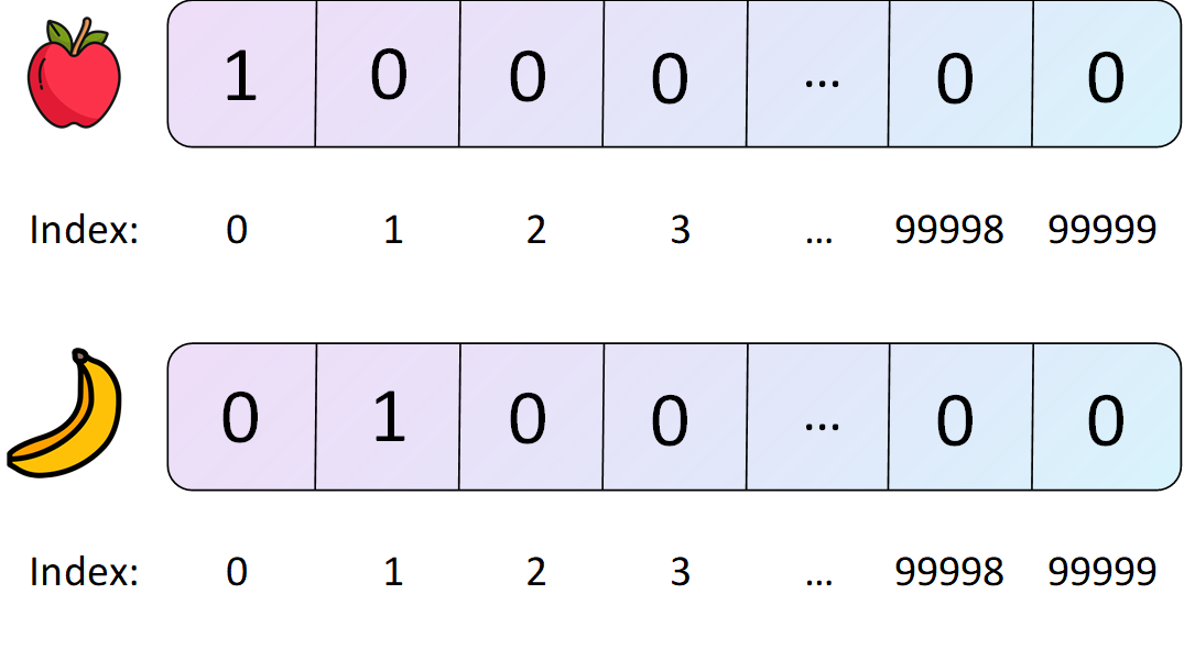
Vocabulary: ["king", "banana", "apple"]
One-hot representation of "king": [1, 0, 0]
One-hot representation of "banana": [0, 1, 0]
One-hot representation of "apple": [0, 0, 1]
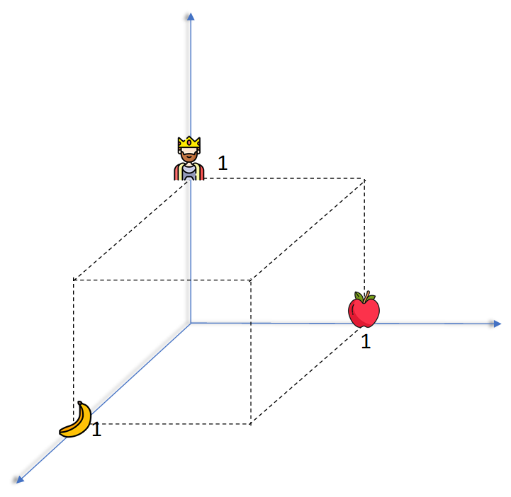
This representation doesn’t capture the relationship between “banana” and “apple” or that both are fruit. Hence, we need better methods like word embeddings.
Using Word Embeddings
Word embeddings are dense vector representations of words in a continuous vector space, where semantically similar words are mapped closer together.
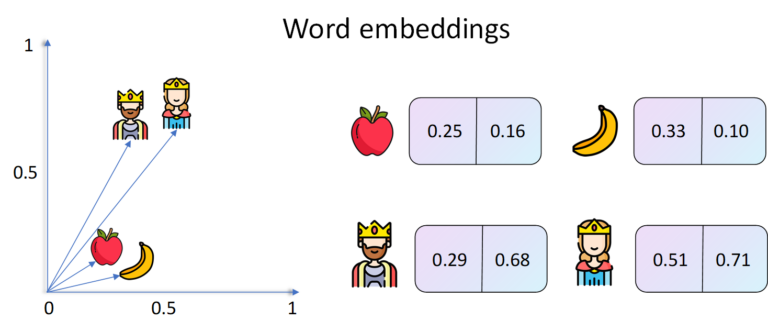
Example: A 3D visualization might show vectors such that:
- vector(“king”) - vector(“man”) + vector(“woman”) ≈ vector(“queen”)
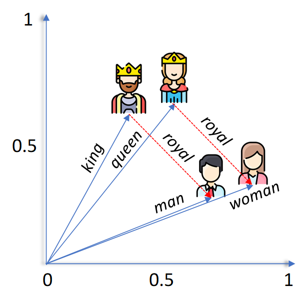
This arithmetic reflects the semantic relationship between the words, allowing machines to understand analogies.
Properties of Word Embeddings
Word embeddings exhibit fascinating properties:
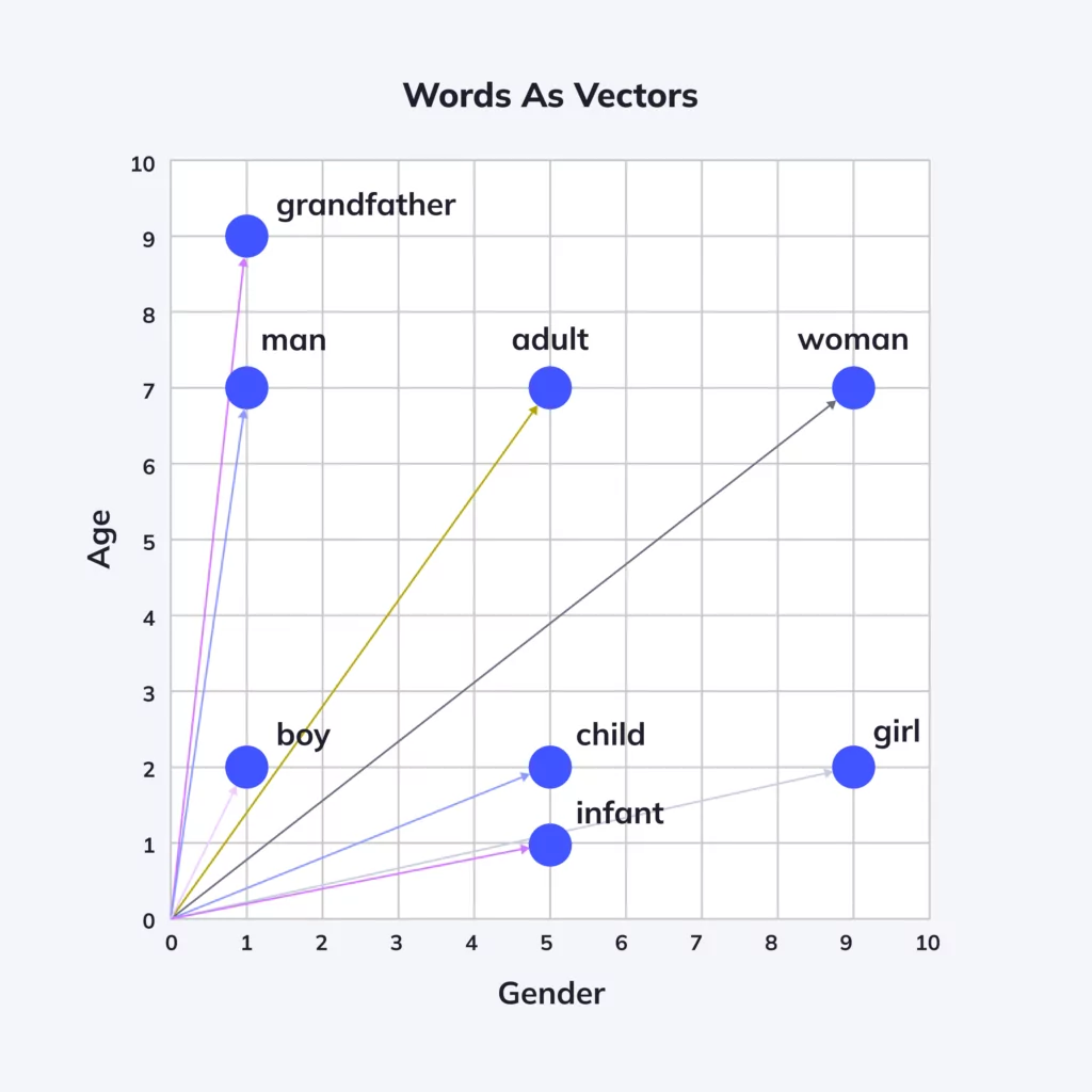
- Semantic similarity: Similar words have vectors close to each other (e.g., “good” and “great”).
- Linear substructures: Relationships can be captured with simple vector arithmetic (e.g., “Paris” - “France” + “Italy” ≈ “Rome”).
- Dimensionality reduction: Embeddings reduce high-dimensional one-hot vectors to lower-dimensional dense vectors (e.g., from 10,000 to 300 dimensions).
Embedding Matrix
An embedding matrix is a trainable matrix in a neural network where each row corresponds to a word’s vector.
Structure:
- Suppose the vocabulary size is
V = 10,000and the embedding size isN = 300. - The embedding matrix
Ewill have shape(V, N).
To retrieve the embedding of word i, simply use:
embedding_vector = E[i]
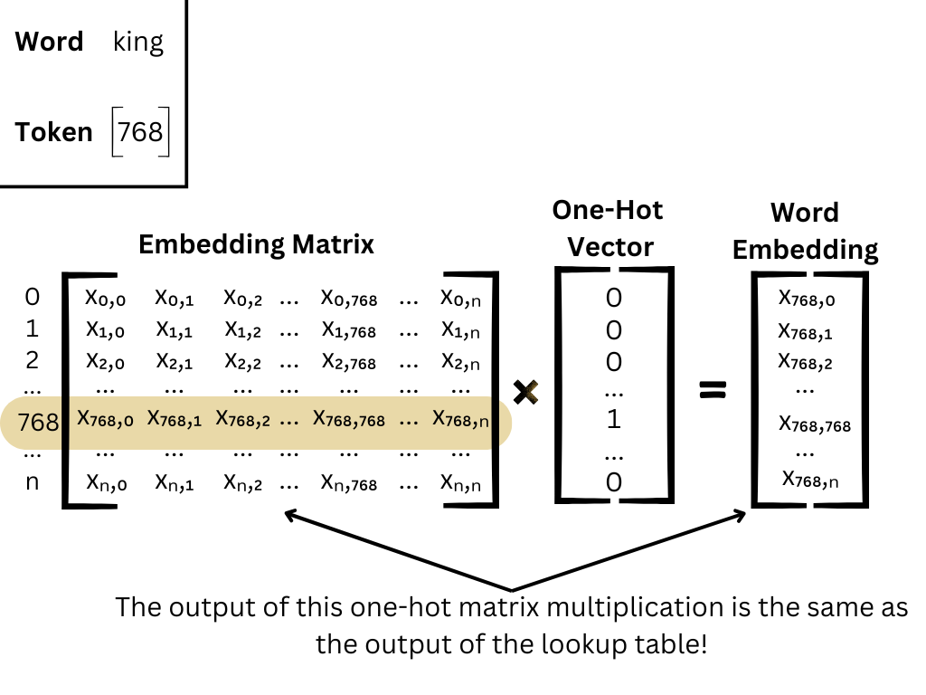
This matrix is updated during training so that embeddings capture task-specific information.
Learning Word Embeddings
Word embeddings can be learned in two ways:
- Supervised Learning: Train a model on a downstream task (e.g., sentiment classification) and update embeddings during training.
- Unsupervised Learning: Train embeddings on large text corpora to learn general-purpose representations (e.g., Word2Vec, GloVe).
Word2Vec
Word2Vec is a popular unsupervised model for learning word embeddings. It has two architectures:
Architectures: CBOW vs Skip-Gram
Word2Vec comes in two main model architectures:
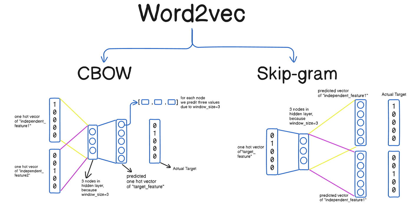
-
Continuous Bag of Words (CBOW):
Predicts the current word based on its context.
Given the surrounding words, the model tries to guess the center word.
Efficient for larger datasets and more frequent words.Example:
- Input: [“the”, “cat”, “on”, “the”, “mat”]
- Center Word: “sat”
- Context: [“the”, “cat”, “on”, “the”, “mat”]
- CBOW tries to predict “sat” from the context.
-
Skip-Gram:
Predicts surrounding context words given the current word.
Given the center word, the model tries to predict the context.
Performs well with smaller datasets and rare words.Example:
- Input: “sat”
- Target Outputs: [“the”, “cat”, “on”, “the”, “mat”]
- Skip-Gram tries to predict the surrounding words from “sat”.
How Word2Vec Learns Word Embeddings
- Word2Vec uses a shallow neural network with one hidden layer.
- The vocabulary size is
V, and the desired vector size isN. - The input layer is a one-hot vector of size
V. - The hidden layer (no activation function) has size
N. - The output layer is also of size
V, predicting a probability distribution over all words.
Steps:
- Convert the input word into a one-hot encoded vector.
- Multiply it by the input weight matrix to get the hidden layer representation.
- Multiply that by the output weight matrix to get scores for all words in the vocabulary.
- Apply softmax to produce a probability distribution.
- Update weights via backpropagation using gradient descent to minimize the loss.
Training Objective: Maximizing Log Probability
For the Skip-Gram model, the goal is to maximize the average log probability:
$$ \frac{1}{T} \sum*{t=1}^{T} \sum*{-m \leq j \leq m, j \neq 0} \log p(w_{t+j} | w_t) $$
Where:
- $ T $ is the total number of words in the corpus.
- $ m $ is the context window size.
- $ wt $ is the center word, and $ w{t+j} $ are the context words.
Computational Challenge: Softmax and Large Vocabulary
Calculating the softmax over a large vocabulary is computationally expensive. To address this, Word2Vec introduces optimization techniques such as:
- Negative Sampling
- Hierarchical Softmax
These methods significantly reduce the training time while maintaining the quality of the learned embeddings.
Example: Learning from a Sentence
Suppose the sentence is:
"The quick brown fox jumps over the lazy dog"
With a context window of size 2, for the center word “brown”, the context is [“The”, “quick”, “fox”, “jumps”].
In the Skip-Gram model, we would train the network to predict each of those context words from “brown”.
Why Word2Vec Works
Word2Vec learns useful representations because:
- It captures both syntactic and semantic relationships.
- It leverages co-occurrence statistics of words in a corpus.
- The vector space preserves many linguistic regularities.
For instance:
vec("Paris") - vec("France") + vec("Italy") ≈ vec("Rome")vec("walking") - vec("walk") + vec("swim") ≈ vec("swimming")
Applications of Word2Vec
- Text classification
- Sentiment analysis
- Named entity recognition
- Question answering
- Semantic search
- Machine translation
These embeddings can be pre-trained (e.g., on Google News) or trained on custom corpora to tailor them to specific domains (e.g., medical texts, legal documents).
Negative Sampling
In Word2Vec, instead of updating weights for all words in the vocabulary, negative sampling updates only a few:
- Pick one positive pair (word and context).
- Sample
knegative words randomly.
This improves efficiency dramatically and allows the model to scale to large corpora.
Loss function (simplified):
$$ \log(\sigma(v_c \cdot v_w)) + \sum_{j=1}^k \mathbb{E}{w_j \sim P_n(w)}[\log(\sigma(-v{w_j} \cdot v_w))] $$
Where:
v_wis the input word vectorv_cis the context vectorP_n(w)is the noise distribution
GloVe Word Vectors
GloVe (Global Vectors for Word Representation) is an alternative to Word2Vec. It constructs a co-occurrence matrix X and models the relationships between words based on their global co-occurrence statistics.
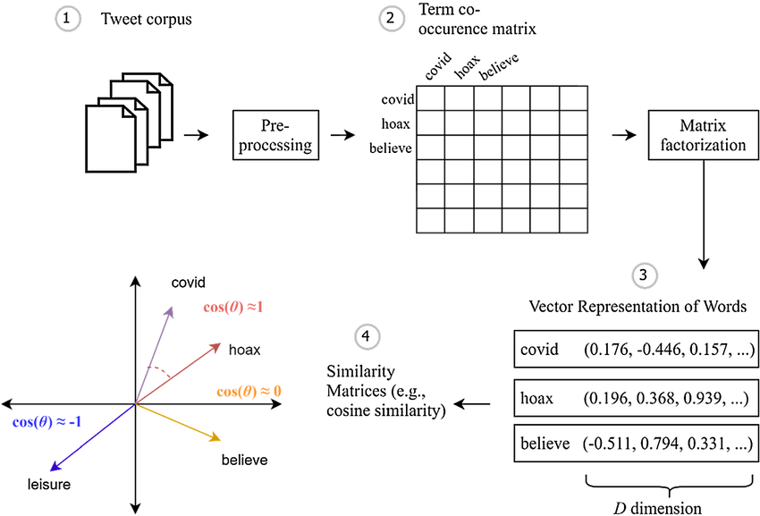
Cost function:
$$ J = \sum_{i,j=1}^{V} f(X_{ij})(w_i^T \tilde{w}_j + b_i + \tilde{b}j - \log X{ij})^2 $$
Where:
- $X_ij$ = number of times word $i$ co-occurs with word $j$
- $w_i$, $\tilde{w}_j$ = word vectors
- $b_i$, $\tilde{b}_j$ = biases
- $f(X)$ = weighting function
This approach captures both local and global word relationships.
Sentiment Classification
Word embeddings can be used as inputs to models like LSTM or CNN for tasks such as sentiment analysis.
Example workflow:
- Convert text to sequence of embeddings.
- Feed sequence into an LSTM.
- Predict a sentiment label: positive, negative, or neutral.
Embeddings help capture contextual sentiment information that traditional methods might miss.
Debiasing Word Embeddings
Word embeddings can reflect and amplify societal biases (e.g., gender bias).
Example:
- vector(“doctor”) might be closer to vector(“man”) than vector(“woman”) in biased embeddings.
Debiasing Techniques:
- Identify bias subspace: e.g., direction of gender (he-she).
- Neutralize: Make gender-neutral words (e.g., “doctor”) orthogonal to the gender direction.
- Equalize: Adjust word pairs (e.g., “man” and “woman”) to be equidistant from neutral terms.
These techniques are essential to make NLP applications fair and inclusive.
This concludes a comprehensive overview of word embeddings and their usage in natural language processing. Each concept here forms the foundation for more advanced NLP models such as Transformers and BERT.
Content

∴
I completed the First Principles of Computer Vision Specialization by taking detailed notes and summarizing critical concepts for future reference.
Columbia University
Course & Note Overview
These notes document my systematic study of the First Principles of Computer Vision specialization taught by Prof. Shree K. Nayar at Columbia University. The notes bridge physical optics, sensor physics, 3D projective geometry, and modern machine perception to build a complete bottom-up understanding of how computers interpret the visual world.
| # | Course / Area | Core Focus & Note Contents |
|---|---|---|
| 1 | Introduction to Computer Vision | Computational vision foundations, human visual pathways, pixel representation, and foundational image pipelines. |
| 2 | Imaging & Sensor Physics | Pinhole camera models, optics & depth of field, CCD/CMOS sensor noise, dynamic range, HDR imaging, and Fourier frequency filtering. |
| 3 | Features & Boundaries | Gradient operators, Canny edge detection, Hough transforms, SIFT keypoints & descriptors, homography, RANSAC, and image stitching. |
| 4 | 3D Reconstruction (Single View) | Radiometry & BRDF reflectance models, photometric stereo, shape from shading, depth from defocus, and active structured light. |
| 5 | 3D Reconstruction (Multi-View) | Epipolar geometry, stereo disparity, multi-view 3D reconstruction, Structure from Motion (SfM), and optical flow motion estimation. |
| 6 | Perception & Visual Learning | Color spaces, human visual perception, neural networks for vision, feature hierarchies, and modern visual recognition. |
— emreaslan —
Introduction to Computer Vision
- 1. What is Computer Vision?
- 2. The Human Visual System: Biology, Fallibility, and Ambiguity
- 3. Topics Covered: Roadmap
- 4. Global Applications: Computer Vision in the Modern World
1. What is Computer Vision?
Computer vision is not merely a subset of artificial intelligence; it is a profound multidisciplinary engineering and scientific enterprise. It bridges the physical world and symbolic understanding, drawing upon optics, signal processing, electrical engineering, and computer science.
Vision pipeline: light source → scene → camera → Vision Software produces a scene description
The fundamental challenge lies in transforming raw numerical arrays—pixel data—into a meaningful description of the 3D environment.
Raw visual input: two children showering
Same scene as a numerical pixel matrix
In this field, the definition of the mission often dictates the methodology. Below is a comparison of the three primary philosophical pillars of computer vision research:
| Perspective | Proponent | Core Philosophy |
|---|---|---|
| Vision as Emulation | David Marr | Aimed at automating human visual processes to replicate the sophistication of biological systems |
| Vision as Information Processing | Berthold Horn | Defined as the task of “inverting” image formation—mathematically walking back from a 2D projection to 3D reality |
| Vision as a Functional Tool | Takeo Kanade | Emphasizes that vision is “fun” but, more importantly, “useful,” serving as a bridge between pure research and practical application |
1.1 The “First Principles” Philosophy
While contemporary deep learning provides powerful tools, a First Principles approach—focusing on mathematical and physical underpinnings—is the prerequisite for generalizable and explainable AI. Relying on “black box” models often bypasses the structural understanding required for true innovation.
Why First Principles? Physical phenomena can be described with elegant math, making massive datasets and exhaustive training cycles unnecessary.
We prioritize these fundamentals for four reasons:
- Precision and Conciseness — Physical phenomena can often be described with elegant math, rendering massive datasets unnecessary.
- Debugging and Diagnostics — When a vision system fails, first principles provide the only rigorous framework for diagnosing the failure.
- Synthetic Data Generation — When real-world data collection is impractical or dangerous, mathematical models allow us to synthesize high-fidelity training data.
- Scientific Curiosity — The innate human drive to understand the “why” behind visual phenomena leads to breakthroughs that purely data-driven methods overlook.
2. The Human Visual System: Biology, Fallibility, and Ambiguity
Studying the human eye is a necessary starting point for designing artificial vision. Even though machines and humans often have divergent goals—qualitative navigation versus quantitative measurement—the eye provides a blueprint for efficient information reduction.
2.1 The Biological Pathway
The human visual system is a complex hierarchy designed for rapid analysis:
flowchart LR
A["👁️ Eye & Lens<br/><i>Primary optical stage</i>"] --> B["🧬 Retina<br/><i>Early processing + data reduction</i>"]
B --> C["🔌 Optic Nerve<br/><i>High-speed conduit</i>"]
C --> D["🧠 LGN<br/><i>Relay station, directs to regions</i>"]
D --> E["🎯 Visual Cortex<br/><i>Shape, color, motion, texture</i>"]
style A fill:#1a1a2e,stroke:#e94560,color:#fff
style B fill:#16213e,stroke:#e94560,color:#fff
style C fill:#0f3460,stroke:#e94560,color:#fff
style D fill:#1a1a2e,stroke:#e94560,color:#fff
style E fill:#16213e,stroke:#e94560,color:#fff
Biological vision pathway: retina → LGN → visual cortex (V1, V2, MT/V5, V8)
2.2 Qualitative vs. Quantitative Vision
As engineers, we must recognize that human vision is a qualitative system, whereas factory automation, medical imaging, and robotics require quantitative precision. A human can recognize a face instantly but cannot measure the length of a component to the nearest millimeter. For tasks requiring extreme reliability, emulating human biology is often the “wrong” goal; machines must provide the measurable accuracy that biological systems lack.
2.3 Case Studies in Visual Illusions
Human vision is more fallible than it appears, often relying on internal assumptions to resolve ambiguity.
Example — Dongary Wave Illusion: The static leaf pattern below appears to shimmer or move due to involuntary micro-saccades of the eye.
Static leaf pattern that produces a perception of motion — the Dongary Wave illusion
| Illusion | What It Reveals |
|---|---|
| Fraser’s Spiral | Concentric circles misinterpreted as a spiral |
| Adelson’s Checker Shadow | Brain compensates for illumination — two identical gray patches look different |
| Dongary Wave | Perceived motion from a static image due to involuntary eye movements |
| Ames Room | Perspective and relative size create an illusion where people appear to grow or shrink |
| Necker Cube / Faces vs. Vase | A single 2D image supports multiple 3D or symbolic interpretations |
| The Crater Illusion | The “lighting from above” assumption — flipping a mound makes it appear as a crater |
| Kanizsa Triangle | The brain “fills in” data (thinking) rather than just processing pixels (seeing) |
Key Insight: While humans think through their visual experiences, machines must first learn to calculate through the rigorous lens of radiometry and geometry.
3. Topics Covered: Roadmap
This specialization covers the entire pipeline — from pixels to perception — organized into six modules:
flowchart TB
subgraph Foundations["🟦 Foundations"]
direction TB
A["Introduction<br/><i>What is CV, human vision</i>"]
B["Imaging<br/><i>Formation, sensors, processing</i>"]
end
subgraph Features["🟧 Features & 2D"]
C["Features<br/><i>Edges, SIFT, stitching, faces</i>"]
end
subgraph Reconstruction["🟩 3D Reconstruction"]
D["Reconstruction I<br/><i>Radiometry, photometric stereo</i>"]
E["Reconstruction II<br/><i>Stereo, optical flow, SfM</i>"]
end
subgraph Perception["🟥 Perception"]
F["Perception<br/><i>Tracking, segmentation, NN</i>"]
end
A --> B --> C --> D --> E --> F
style A fill:#1a1a2e,stroke:#4cc9f0,color:#fff
style B fill:#1a1a2e,stroke:#4cc9f0,color:#fff
style C fill:#1a1a2e,stroke:#f72585,color:#fff
style D fill:#1a1a2e,stroke:#06d6a0,color:#fff
style E fill:#1a1a2e,stroke:#06d6a0,color:#fff
style F fill:#1a1a2e,stroke:#e94560,color:#fff
style Foundations fill:transparent,stroke:#4cc9f0,color:#4cc9f0
style Features fill:transparent,stroke:#f72585,color:#f72585
style Reconstruction fill:transparent,stroke:#06d6a0,color:#06d6a0
style Perception fill:transparent,stroke:#e94560,color:#e94560
Module Breakdown
| # | Module | Focus |
|---|---|---|
| 1 | Imaging | Image formation, sensors, binary images, image processing (convolution, Fourier) |
| 2 | Features | Edge/boundary detection, SIFT, image stitching, face detection |
| 3 | Reconstruction I | Radiometry, photometric stereo, shape from shading, depth from defocus |
| 4 | Reconstruction II | Camera calibration, stereo, optical flow, structure from motion |
| 5 | Perception | Object tracking, segmentation, appearance matching, neural networks |
4. Global Applications: Computer Vision in the Modern World
Vision has evolved from a laboratory curiosity into a thriving global industry across diverse sectors.
| Domain | Applications |
|---|---|
| Industrial / Efficiency | Factory automation, high-speed visual inspection, OCR for license plates and postal scanning |
| Security / Identity | Biometrics using iris patterns (as unique as DNA), robust face recognition |
| Consumer Tech | Optical mice (mini-vision systems), gaming (Kinect / PlayStation), AR (Snapchat 3D mesh filters) |
| Intelligent Marketing | Vending machines detecting customer demographics (age/gender) to display targeted products |
| Visual Search | Instant identification of monuments and objects via mobile devices |
| Advanced Mobility | Driverless cars using sensor fusion, Mars Rover terrain mapping |
| Creative / Medical | Motion capture for cinema, medical diagnostics (X-ray, MRI, ultrasound) |
Pinhole Camera Model and Perspective Projection
- 1. Introduction to Image Formation
- 2. The Pinhole Camera Model
- 3. Magnification, Vanishing Points, and Visual Manifestations
- 4. The Ideal Pinhole Size
- Summary
1. Introduction to Image Formation
Image formation is the process of projecting the physical properties of a three-dimensional (3D) scene onto a two-dimensional (2D) plane. This process forms the foundation of computer vision and defines the relationship between the position of scene points in the image and their brightness values. To fully understand the process, it is essential to separate geometric and photometric interactions:
- Geometric Relationships — Determine the coordinates of a scene point on the projection plane (where it falls).
- Photometric Relationships — Define the intensity (brightness) at which a scene point appears in the image, based on material properties and lighting conditions.
Theoretically, a simple sensor or screen placed in front of a scene cannot produce a clear image. The fundamental reason is that each point on the sensor receives light rays from many different points in the scene, spreading in a cone shape. This “muddled” state of light rays causes each point to receive the average brightness of the scene, resulting in a blurred accumulation of light rather than a clear visual structure. A pinhole or lens mechanism aims to restrict this light cone and establish a one-to-one mapping between the scene and the sensor.
Key Insight: Without a restricting aperture, every sensor point integrates light from a cone of scene points — producing blur, not image.
2. The Pinhole Camera Model
The pinhole camera model is the simplest way to prevent the “muddled” image by forcing all light rays to pass through a single point. This model forms the basis of the perspective projection equations — the single most critical concept in computer vision.
2.1 Perspective Projection Equations
In the pinhole model, the optical center (pinhole) is taken as the origin, and the $z$-axis is placed on the optical axis perpendicular to the image plane. The distance between the pinhole and the image plane is called the effective focal length ($f$). Using the principle of similar triangles, the projection $P_i(x_i, y_i, f)$ of a scene point $P_o(x_o, y_o, z_o)$ onto the image plane is given by:
$$ \frac{x_i}{f} = \frac{x_o}{z_o} \quad \text{and} \quad \frac{y_i}{f} = \frac{y_o}{z_o} $$
These equations mathematically prove that:
- The image is always inverted.
- The size of objects is inversely related to depth ($z_o$).
$$ x_i = f \frac{x_o}{z_o}, \qquad y_i = f \frac{y_o}{z_o} $$
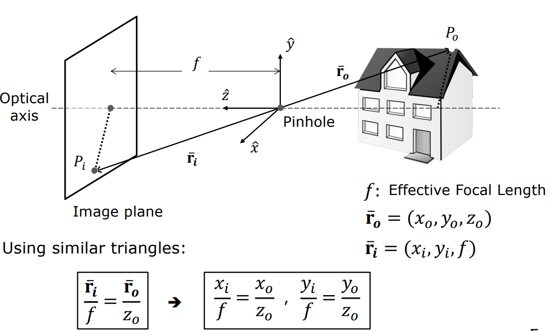
flowchart LR
A["Scene Point<br/>P_o(x_o, y_o, z_o)"] -->|"Light ray"| B["Pinhole<br/>(Optical Center)"]
B -->|"Projection"| C["Image Plane<br/>P_i(x_i, y_i, f)"]
D["Focal Length f"] -.- B
style A fill:#1a1a2e,stroke:#e94560,color:#fff
style B fill:#16213e,stroke:#e94560,color:#fff
style C fill:#0f3460,stroke:#4cc9f0,color:#fff
style D fill:#1a1a2e,stroke:#888,color:#888
2.2 Historical Milestones
flowchart LR
A["500 BCE<br/>Chinese philosophers describe pinhole"] --> B["1000 CE<br/>Alhazen analyzes camera obscura"]
B --> C["1544<br/>Gemma Frisius observes solar eclipse"]
C --> D["Natural<br/>Nautilus pompilius pinhole eye"]
style A fill:#1a1a2e,stroke:#e94560,color:#fff
style B fill:#16213e,stroke:#4cc9f0,color:#fff
style C fill:#0f3460,stroke:#f72585,color:#fff
style D fill:#1a1a2e,stroke:#06d6a0,color:#fff
2.3 Natural Pinhole: The Nautilus Eye
The Nautilus pompilius is a remarkable example of pinhole imaging in nature. Unlike most cephalopods, the nautilus evolved a lensless eye that works exactly like a pinhole camera. The small aperture produces a sharp image with infinite depth of field, but at the cost of light sensitivity — a fundamental trade-off that appears throughout optical design.
3. Magnification, Vanishing Points, and Visual Manifestations
The geometric changes in an image are direct consequences of perspective projection. These shape our depth perception and the 2D representation of 3D scenes.
3.1 Image Magnification
Magnification is the ratio of the image size to the scene size:
$$ |m| = \frac{f}{z_o} $$
The inverse relationship between magnification and depth ($z_o$) is why:
- Railroad tracks appear to converge at the horizon.
- Selfies make the nose appear much larger than the ears — the nose has a smaller $z_o$ value, creating a natural distortion.
3.2 Vanishing Points
All lines that are parallel in 3D space converge to a single point in the 2D image plane.
To find this point, construct a ray passing through the pinhole parallel to these lines (in direction $L_x, L_y, L_z$). The coordinates where this ray pierces the image plane are:
$$ x_{vp} = f \cdot \frac{L_x}{L_z}, \qquad y_{vp} = f \cdot \frac{L_y}{L_z} $$
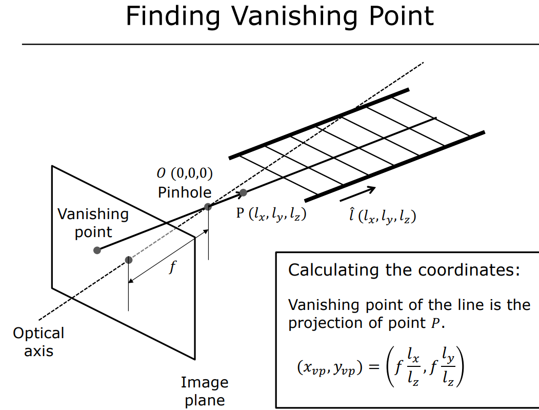
3.3 Artistic and Architectural Applications
| Artist/Architect | Work | Technique |
|---|---|---|
| Vermeer | “The Music Lesson” | Placed the vanishing point exactly at the student’s elbow, directing attention to the piano-playing activity |
| Borromini | “Galleria Spada” | Created false perspective by shrinking columns and lowering the ceiling — a 30-meter corridor appears to be 150 meters long |
Key Insight: Perspective projection is not just a mathematical constraint — it is a tool for visual storytelling, exploited by artists long before computer vision formalized it.
4. The Ideal Pinhole Size
While the pinhole model produces sharp images, the aperture size introduces a critical trade-off: a smaller pinhole reduces blur but also reduces light, while a larger pinhole collects more light but increases image blur. This fundamental limitation motivates the transition from pinholes to lens-based imaging systems.
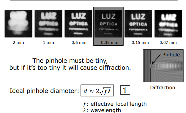
Summary
- Image formation requires restricting light rays through an aperture to avoid the “muddled” cone problem.
- The pinhole camera model produces perspective projection governed by similar triangles: $x_i/f = x_o/z_o$.
- Magnification is inversely proportional to depth: objects farther away appear smaller.
- Vanishing points are where parallel lines in 3D converge in a 2D projection.
- The pinhole’s primary limitation is light collection — this motivates the use of lenses.
Lens Systems and Depth of Field
1. Why Lenses?
Pinhole cameras produce sharp images, but the extremely small aperture collects very little light — the Flatiron building example required a 12-second exposure. Lenses solve this problem by refracting light from a wide aperture to converge at a single point, increasing brightness while preserving the perspective model.
Fundamental Trade-off: Lenses collect more light but introduce a finite depth of field — only one plane is perfectly in focus.
2. Gaussian Lens Law
For a thin lens, the relationship between the object distance ($o$), image distance ($i$), and focal length ($f$) is given by the Gaussian Lens Law:
$$ \frac{1}{i} + \frac{1}{o} = \frac{1}{f} $$
flowchart LR
A["Object<br/>Distance o"] --> B["Thin Lens<br/>Focal Length f"]
B --> C["Image<br/>Distance i"]
D["1/f = 1/i + 1/o"] -.- B
style A fill:#1a1a2e,stroke:#e94560,color:#fff
style B fill:#16213e,stroke:#4cc9f0,color:#fff
style C fill:#0f3460,stroke:#e94560,color:#fff
style D fill:#1a1a2e,stroke:#888,color:#888
Numerical Example: With a lens of $f = 50$mm focused on an object at $o = 300$mm:
$$ \frac{1}{i} = \frac{1}{50} - \frac{1}{300} = \frac{6 - 1}{300} = \frac{5}{300} $$
$$ i = 60 \text{ mm} $$
The image forms 60 mm behind the lens.
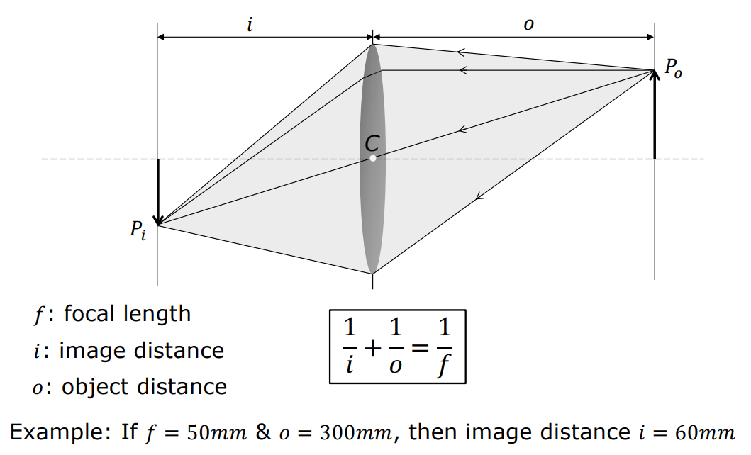
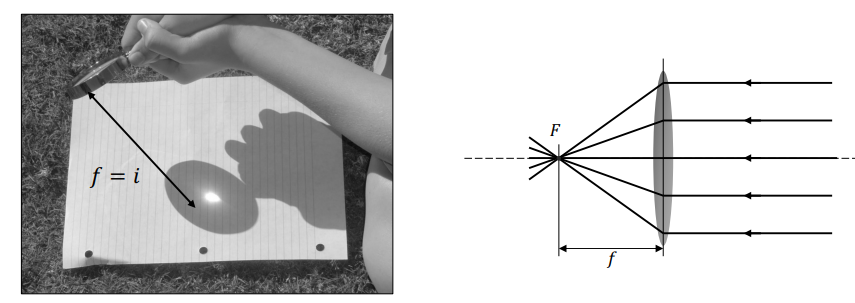
2.1 Aperture and f-Number
The light-gathering capacity of a lens is determined by the aperture diameter ($D$). The f-number ($N$) is defined as:
$$ N = \frac{f}{D} $$
| Aperture | f-Number | Light Collected | Depth of Field |
|---|---|---|---|
| Wide open | Low $N$ (e.g., $f/1.4$) | High | Shallow |
| Stopped down | High $N$ (e.g., $f/16$) | Low | Deep |
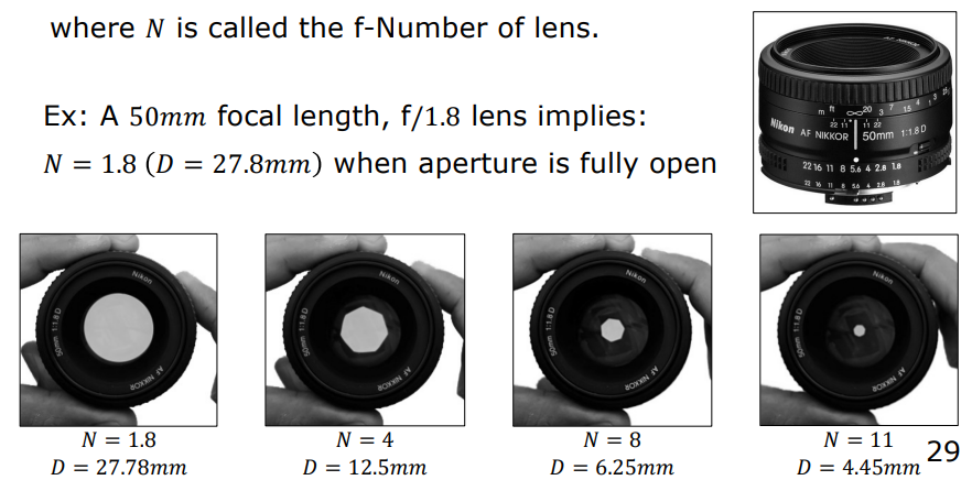
2.2 The Tissue Box Experiment
A fascinating and counter-intuitive observation: covering half of a lens does not break or defocus the image. It only reduces the light reaching the sensor, darkening the image. Every unblocked portion of the lens continues to project the entire scene onto the focal plane.
Why? Each point on the lens receives light from all scene points within its field of view. Blocking part of the lens reduces the number of rays but does not change their geometric paths — the entire scene is still projected, just dimmer.
2.3 Zoom
Zoom is the process of changing the magnification by moving lens elements within a multi-lens system. This changes the effective focal length without physically swapping lenses.
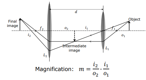
3. Defocus Blur and Depth of Field
A lens system perfectly focuses only a single focal plane at a specific sensor position. Points outside this plane form a blur circle (circle of confusion) on the image plane.

3.1 The Blur Circle
Using similar triangles, the diameter of the blur circle ($b$) is related to the aperture diameter ($D$):
$$ \frac{b}{D} = \frac{|i’ - i|}{i’} $$
Where $i’$ is the image distance of the out-of-focus point, and $i$ is the sensor distance.
flowchart LR
subgraph InFocus["In Focus"]
A1["Scene Point on Focal Plane"] --> B1["Lens"] --> C1["Sharp Point on Sensor"]
end
subgraph OutOfFocus["Out of Focus"]
A2["Scene Point off Focal Plane"] --> B2["Lens"] --> C2["Blur Circle on Sensor"]
end
style A1 fill:#16213e,stroke:#4cc9f0,color:#fff
style B1 fill:#1a1a2e,stroke:#4cc9f0,color:#fff
style C1 fill:#0f3460,stroke:#4cc9f0,color:#fff
style A2 fill:#16213e,stroke:#e94560,color:#fff
style B2 fill:#1a1a2e,stroke:#e94560,color:#fff
style C2 fill:#0f3460,stroke:#e94560,color:#fff
This equation proves that the blur circle diameter is directly proportional to the aperture diameter — wider apertures produce more defocus blur.
3.2 Depth of Field (DoF)
The Depth of Field is the range of depths over which the blur circle diameter remains smaller than the pixel size ($C$). If $b < C$, the image is perceived as “sharp.”
$$ \text{DoF} \propto \frac{N \cdot C \cdot o^2}{f^2} $$
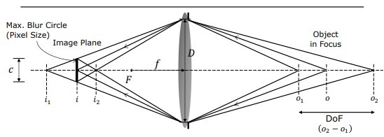
3.3 Hyperfocal Distance
The hyperfocal distance ($H$) is the focus distance at which everything from that point to infinity appears acceptably sharp:
$$ H = \frac{f^2}{N \cdot C} + f $$
Smartphone cameras strategically use this parameter — their small sensors and short focal lengths produce a very large hyperfocal distance, ensuring nearly everything is in focus without active focusing.
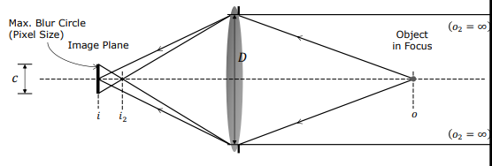
3.4 The Critical Trade-off
| Scenario | Aperture | Light | Exposure Time | Depth of Field |
|---|---|---|---|---|
| Bright, shallow DoF | Wide ($N$ low) | High | Short | Shallow |
| Dark, deep DoF | Narrow ($N$ high) | Low | Long | Deep |
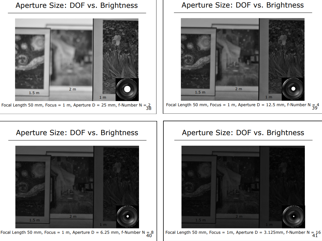
There is no free lunch in optical design — every gain in one dimension comes at a cost in another.
Summary
- Lenses increase light collection but introduce finite depth of field.
- Gaussian Lens Law: $1/i + 1/o = 1/f$ governs thin lens behavior.
- f-Number $N = f/D$ quantifies aperture size and directly affects light and DoF.
- Blur circle $b/D = |i’ - i|/i’$ proves defocus is proportional to aperture.
- Hyperfocal distance $H = f^2/(N \cdot C) + f$ enables strategic focus optimization.
- The aperture trade-off (light vs. DoF) is fundamental and unavoidable.
Advanced Optical Systems: Aberrations, Wide-Angle Imaging, and Biological Eyes
- 1. Lens Aberrations
- 2. Wide-Angle and Catadioptric Imaging Systems
- 3. Biological Eye Designs and Evolution
- Summary
1. Lens Aberrations
Even perfect lenses produce unwanted effects called aberrations due to the nature of light. These are physical limitations, not manufacturing defects.
1.1 Vignetting
Vignetting is the darkening of image corners caused by:
- The lens body mechanically blocking oblique rays.
- A reduction in solid angle at the periphery of the image field.
The result is a gradual fall-off in brightness from the center to the corners of the image.
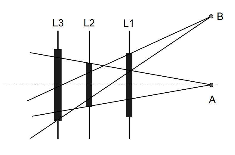
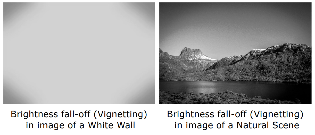
1.2 Chromatic Aberration
The refractive index of glass depends on the wavelength ($\lambda$) of light. In the visible spectrum (400 nm — 700 nm), blue light (400 nm) bends more than red light (700 nm). This causes different colors to focus at different planes, producing color fringing at object edges.
flowchart LR
A["White Light<br/>400-700 nm"] --> B["Lens"]
B --> C["Blue Focus<br/>(shorter focal length)"]
B --> D["Red Focus<br/>(longer focal length)"]
C --> E["Color Fringing at Edges"]
D --> E
style A fill:#1a1a2e,stroke:#fff,color:#fff
style B fill:#16213e,stroke:#4cc9f0,color:#fff
style C fill:#1a1a2e,stroke:#4361ee,color:#4361ee
style D fill:#1a1a2e,stroke:#e94560,color:#e94560
style E fill:#0f3460,stroke:#f72585,color:#fff
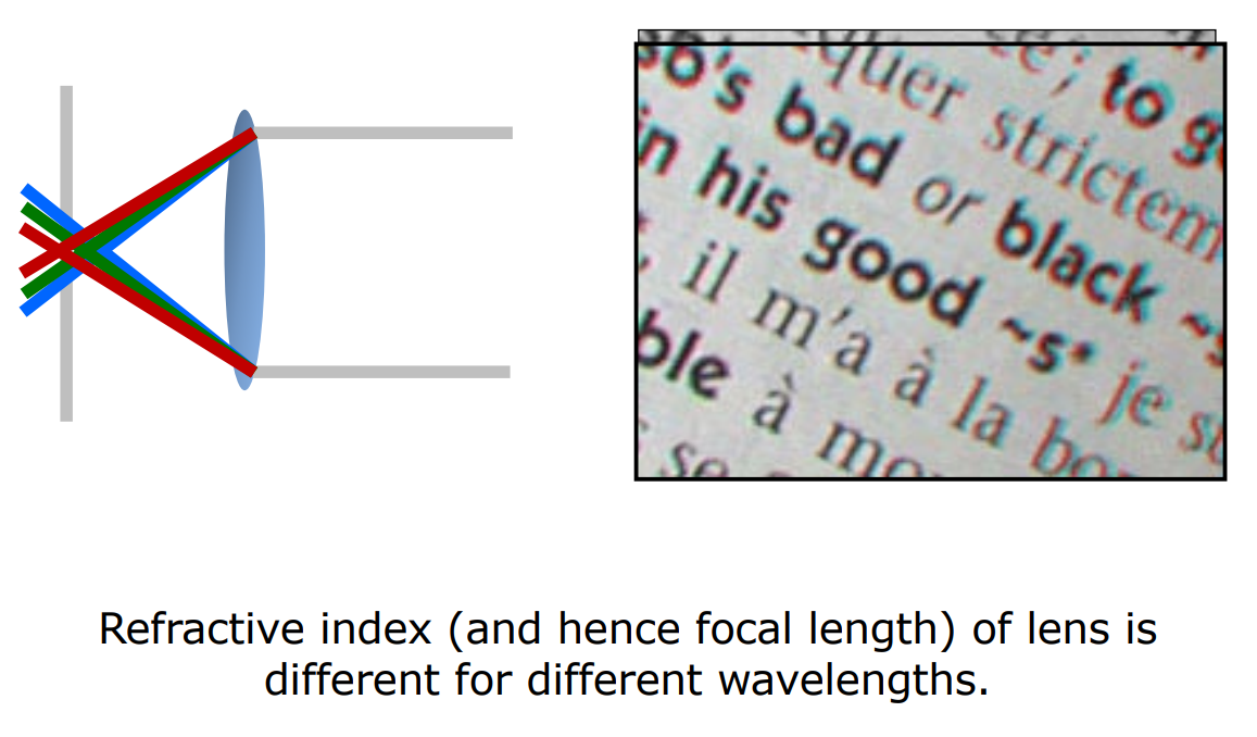
1.3 Geometric Distortions
Radial distortion (barrel distortion) causes the image to bulge outward. These effects can be corrected in computer vision software through inverse mapping — a calibration process that models the distortion parameters and inverts them.
| Distortion Type | Effect | Visual |
|---|---|---|
| Barrel (Fıçı) | Lines bow outward from center | 👁️ Wide-angle look |
| Pincushion (İğne Yastığı) | Lines bow inward toward center | 🔍 Telephoto look |
Key Insight: Distortion is deterministic and correctable — knowing the lens model allows precise geometric rectification.
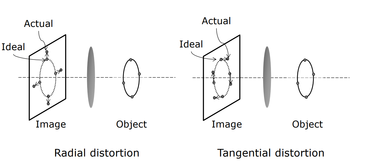
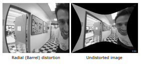
2. Wide-Angle and Catadioptric Imaging Systems
These systems are designed to overcome the limitations of standard perspective projection and are strategically important in security and robotics.
2.1 Fisheye Lenses
Fisheye lenses use meniscus elements to achieve extreme light bending. The single viewpoint constraint is critical for software rectification — all rays must appear to converge at a single optical center for the image to be mathematically unwrapped.
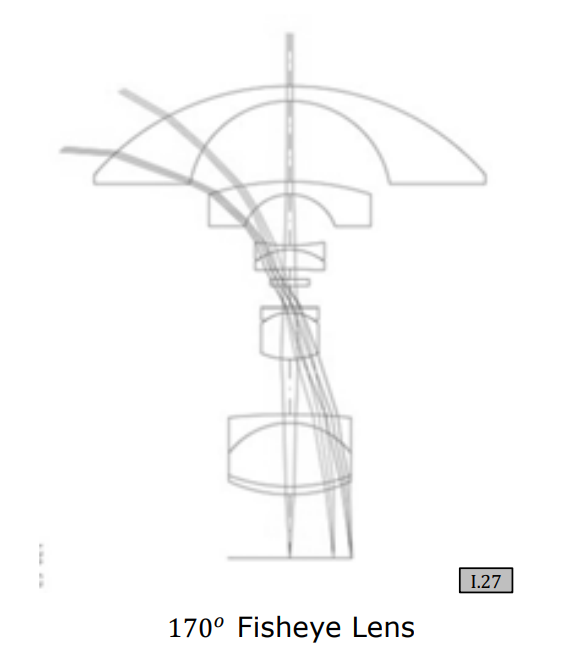
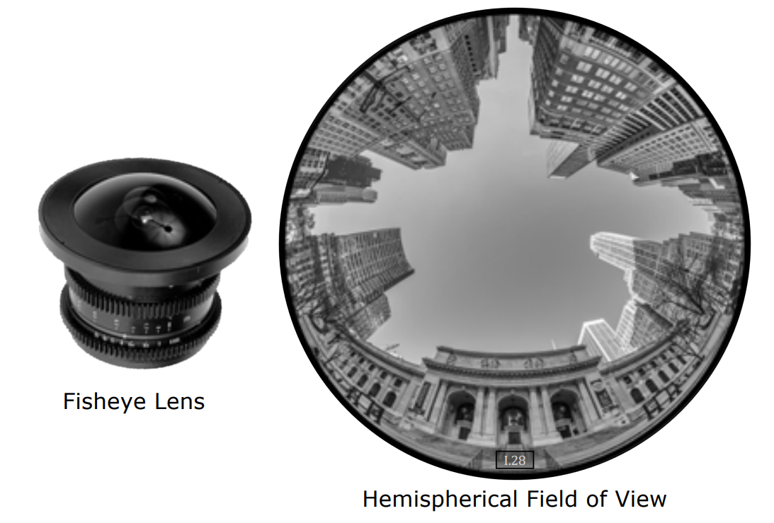
2.2 Catadioptric Systems
Catadioptric systems combine mirrors (catoptric) and lenses (dioptric):
| Type | Mirror Shape | Use Case |
|---|---|---|
| Telescope | Parabolic | Collects parallel rays at a single point |
| Omnidirectional | Hyperbolic (convex) | Captures 360° panoramic view for surveillance |
2.3 Corneal Imaging
The human cornea acts as a convex mirror. Using limbus detection and corneal reflection analysis, it is possible to determine what a person is looking at (their retinal image) from a high-resolution photograph taken from outside.
flowchart LR
A["External Camera"] -->|"High-res photo"| B["Corneal Reflection<br/>Convex mirror"]
B -->|"Limbus detection"| C["Gaze Direction<br/>Analysis"]
C -->|"Inverse projection"| D["Retinal Image<br/>(What person sees)"]
style A fill:#1a1a2e,stroke:#e94560,color:#fff
style B fill:#16213e,stroke:#4cc9f0,color:#fff
style C fill:#0f3460,stroke:#f72585,color:#fff
style D fill:#1a1a2e,stroke:#06d6a0,color:#fff
3. Biological Eye Designs and Evolution
Eyes in nature represent the evolutionary perfection of image formation principles. A simulation by Nilsson demonstrated that a flat, light-sensitive epithelium could evolve into a complex eye in just 400,000 generations.
3.1 The Evolutionary Path
flowchart LR
A["Flat Light-Sensitive Epithelium"] --> B["Curving for Directional Sensitivity"]
B --> C["Aperture Narrowing for Sharpness"]
C --> D["Lens Formation for Light Collection"]
D --> E["Complex Eye"]
style A fill:#1a1a2e,stroke:#4cc9f0,color:#fff
style B fill:#16213e,stroke:#4cc9f0,color:#fff
style C fill:#0f3460,stroke:#f72585,color:#fff
style D fill:#16213e,stroke:#e94560,color:#fff
style E fill:#1a1a2e,stroke:#06d6a0,color:#fff
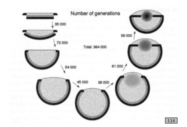
3.2 Comparative Biology
| Species | Eye Type | Key Feature |
|---|---|---|
| Trilobites (400M years ago) | Compound eye | Thousands of calcite crystal lenses |
| Human | Single lens eye | Corneal bending power + crystalline lens accommodation |
| Scallop | Multiple mirror eyes | Concave parabolic mirrors (like James Webb Telescope) |
Fascinating Fact: Trilobite eyes used calcite — a mineral that does not soften with age — as their lens material, giving them perfect vision throughout their lifespan.
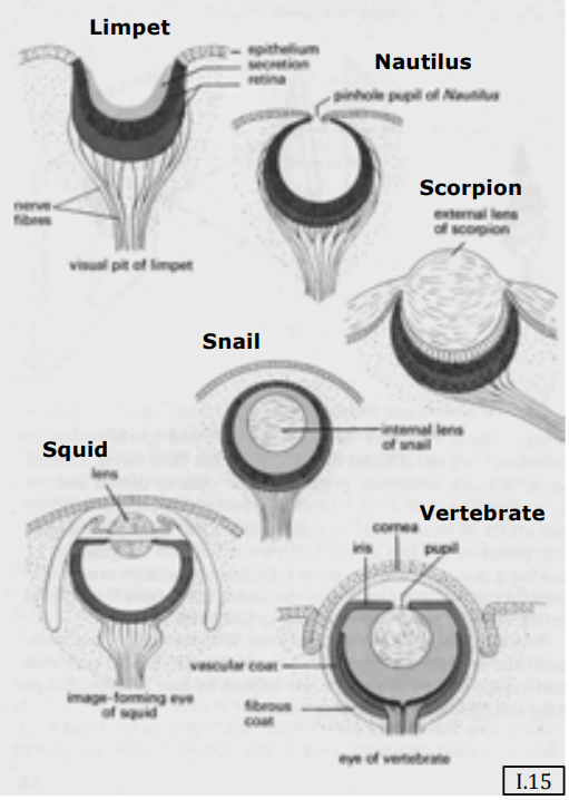
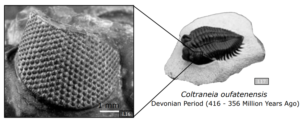
3.3 The Human Eye and Accommodation
The human eye combines two optical elements:
- Cornea — Provides most of the bending power (refractive index difference between air and tissue).
- Crystalline Lens — A fluid-filled flexible lens that adjusts shape for accommodation (focusing at different distances).
As we age, the crystalline lens hardens (presbyopia):
$$ \text{Minimum Focus Distance} \approx \begin{cases} 7 \text{ cm} & \text{at age 10} \ 10 \text{ cm} & \text{at age 20} \ 50 \text{ cm} & \text{at age 50+} \end{cases} $$
3.4 Scallop Eyes: Nature’s Mirror Telescopes
Scallops have hundreds of eyes, each using a concave parabolic mirror rather than a lens to focus light. This is the same optical principle used by the James Webb Space Telescope — a remarkable case of convergent evolution between biology and engineering.
Summary
- Aberrations (vignetting, chromatic, distortion) are unavoidable physical effects of lens systems.
- Catadioptric systems combine mirrors and lenses for specialized imaging (panoramic, telescope).
- Corneal imaging allows gaze detection from external photographs.
- Biological eyes evolved through a well-understood path and offer diverse optical strategies — pinhole (nautilus), compound (trilobite), refractive (human), and reflective (scallop).
- Whether an ancient trilobite lens or a modern liquid lens, image formation is the central achievement of both biological and technological evolution in understanding the 3D world on a 2D plane.
Overview, History, and Image Sensor Types
- 1. Overview
- 2. A Brief History of Imaging
- 2.1 The Pinhole Camera (Camera Obscura)
- 2.2 Lens and Mirror Integration
- 2.3 The Chemical Film Revolution
- 2.4 The Silicon Image Detector (Silicon Detector)
- 2.5 Smartphone Cameras and AI Catalysis
- 2.6 Century-Scale Comparison: Kodak Brownie vs. Modern Smartphone Camera
- 2.7 Future Outlook: Wafer-Scale Integration
- 3. Types of Image Sensors and Solid-State Physics
1. Overview
Image sensing is the physical process of capturing electromagnetic radiation (light) emitted or reflected by a three-dimensional (3D) scene and converting it into a persistent, measurable two-dimensional (2D) representation. While optics (lenses and apertures) govern the geometry of projection, image sensing governs the photometric conversion — mapping incoming photon flux into measurable physical changes, such as chemical reduction in film or electrical charge in solid-state silicon.
Understanding the evolution and physics of image sensors is fundamental to computer vision: every algorithm operating on digital pixels implicitly relies on the optoelectronic properties, sampling limits, dynamic range, and noise characteristics of the underlying sensor architecture.
Key Insight: Optics determine where light rays land on a plane; sensing determines how photon energy is transduced into countable signals (charges or voltages).
2. A Brief History of Imaging
The journey of capturing light and projecting the physical world onto a two-dimensional surface spans centuries of scientific and artistic evolution, moving from passive optical projection to chemical storage, and ultimately to digital silicon architectures.
flowchart TD
T1["500 B.C. — Pinhole Camera<br/>(Camera Obscura)"] --> T2["17th Century — Lens Integration<br/>& Mirror Folding"]
T2 --> T3["1830s — Chemical Film Revolution<br/>(Daguerreotype)"]
T3 --> T4["1970s — Silicon Image Detector<br/>(Reusable Solid-State)"]
T4 --> T5["2000s-Present — Smart Cameras<br/>& Wafer-Scale Integration"]
style T1 fill:#1a1a2e,stroke:#e94560,color:#fff
style T2 fill:#16213e,stroke:#4cc9f0,color:#fff
style T3 fill:#0f3460,stroke:#f72585,color:#fff
style T4 fill:#06d6a0,stroke:#111,color:#000
style T5 fill:#118ab2,stroke:#fff,color:#fff
2.1 The Pinhole Camera (Camera Obscura)
The foundational concept of image formation dates back to 500 B.C., documented by Chinese philosophers who wrote about the principles of the pinhole camera. Around 1000 A.D., Arabian scholar Ibn al-Haytham (Alhazen) analyzed the optical properties and geometric projection of the pinhole camera in rigorous detail.
It was not until the 16th century that the concept gained widespread popularity in the West, particularly among artists. As illustrated in the 1544 sketch by Dutch mathematician Gemma Frisius:
- A minuscule pinhole in a dark room’s wall projects a 3D scene onto an opposing flat wall, creating an inverted 2D image.
- An artist could step into the camera obscura loop, trace the projected image on the wall, and generate geometrically accurate perspective drawings of the 3D scene.
Optics Limitation: While a pinhole camera produces sharp images across infinite depths, its aperture is mathematically tiny, collecting very few photons. The resulting projected images are extremely dim and require dark adaptation to observe.
2.2 Lens and Mirror Integration
To resolve the photon starvation of the pinhole, 17th-century designers replaced the tiny pinhole with a refractive convex lens. The lens successfully focused a significantly larger cone of light, producing dramatically brighter projections.
During the 18th century, optomechanical designs prioritized artist ergonomics:
- The vertical light cone projected by the lens was folded by a $45^\circ$ mirror.
- This redirected the light upward onto a horizontal, translucent sheet of tracing paper.
- The artist could sit comfortably, look downward, and trace the scene — establishing the optomechanical layout that later inspired the Single-Lens Reflex (SLR) viewfinder.
2.3 The Chemical Film Revolution
The most profound cultural leap in imaging occurred in the 1830s with Louis Daguerre’s co-invention of the Daguerreotype camera. Still-life photographs taken in 1837 demonstrated that a scene could be physically recorded on a permanent chemical medium with a single button press, completely removing the human artist from the capture loop.
Chemical Process of Black-and-White Film
- Emulsion: Film is coated with a microscopic layer of light-sensitive silver halide crystals ($\text{AgX}$, where $\text{X} = \text{Br, Cl, I}$).
- Exposure: Photon absorption triggers localized reduction of silver ions to metallic silver: $$\text{Ag}^+ + e^- \xrightarrow{h\nu} \text{Ag}^0$$ The total exposure energy $E$ obeys the reciprocity law: $$\text{Exposure } (E) \propto \text{Irradiance } (I) \times \text{Integration Time } (T)$$
- Development: A chemical bath amplifies this latent metallic silver image, forming a stable, high-resolution photographic negative.
Transition to Color Film (1880s)
Capturing the full visible spectrum required sophisticated multi-layer chemistry. In 1887, Louis Ducos du Hauron captured early color photographs by stacking three separate emulsions with dye couplers containing Red, Green, and Blue pigments.
By the 1920s, consumer cameras like the Ernemann camera entered mass production with slogans like “What you can see, you can photograph,” establishing visual recording as a ubiquitous medium of human expression.
2.4 The Silicon Image Detector (Silicon Detector)
While chemical film revolutionized visual culture, its fundamental limitation was its single-use consumable nature. In the 1970s, the invention of the silicon image detector fundamentally shifted the paradigm:
- Unlike chemical film, a silicon sensor is a reusable solid-state device capable of capturing an infinite sequence of images without chemical processing.
- It took nearly 20 years (until the early 1990s) for silicon manufacturing to mature to consumer viability, yielding early consumer digital cameras such as the Nikon COOLPIX.
- Early digital devices captured resolutions around $640 \times 480$ pixels ($\approx 0.3\text{ MP}$), consumed substantial power, and lacked fast storage, but definitively proved the viability of digital image processing.
2.5 Smartphone Cameras and AI Catalysis
The late 20th and early 21st centuries saw the integration of camera modules into mobile phones, driving unprecedented miniaturization and optical engineering.
- The launch of smartphones in 2007 catalyzed a second digital camera revolution.

- This explosion of mobile cameras birthed global visual communication platforms and generated petabytes of daily image data.
- Crucially, this massive influx of digital imagery served as the core dataset and computational catalyst for modern computer vision and deep learning algorithms.
2.6 Century-Scale Comparison: Kodak Brownie vs. Modern Smartphone Camera
| Specification / Feature | Kodak Brownie Model 1 (1900) | Modern Smartphone Camera Module |
|---|---|---|
| Retail Price | $1.00 USD (Approx. $30.00 adjusted) | Highly optimized mass-production cost |
| Optics Geometry | Single spherical glass lens element | Multi-element, ultra-thin molded aspherical plastic/glass lenses |
| Focusing Mechanism | Fixed-focus system (no adjustment) | Dynamic autofocus via micro voice coil motor (VCM) with micron precision |
| Aperture Control | Slide-in metal plate with discrete holes | Miniaturized micro-diaphragm arrays or fixed low F-number apertures ($f/1.5 - f/1.8$) |
| Viewfinder & Feedback | Small reflective corner mirror (no sensor feed) | Real-time digital display showing live electronic sensor feed |
| Medium / Latency | Silver halide roll film; mailing required; weeks of latency | Silicon sensor; on-board ISP; instant visualization and zero-shutter-lag capture |
2.7 Future Outlook: Wafer-Scale Integration
The next paradigm shift in sensor design involves Optics-on-Wafer and 3D-Stacked Sensor technology:
flowchart TD
A["1. Refracting Microlens & Lenslet Array<br/>(Grown directly on semiconductor wafer)"] --> B["2. Color Filter & Photodiode Array<br/>(Top Silicon Sensing Layer)"]
B --> C["3. 3D Stacked Micro-Electronics Substrate<br/>(Direct Hybrid Bonding)"]
C --> D["4. On-Chip Neural Processing Unit (NPU)<br/>& ISP Execution Engine"]
style A fill:#1a1a2e,stroke:#4cc9f0,color:#fff
style B fill:#16213e,stroke:#e94560,color:#fff
style C fill:#0f3460,stroke:#f72585,color:#fff
style D fill:#06d6a0,stroke:#111,color:#000
- Instead of mounting separate molded plastic lenses over a finished sensor, refracting lens elements are grown directly on top of the silicon wafer at the semiconductor foundry.
- 3D stacked electronics are fabricated directly into the silicon substrate beneath the sensing layer.
- This places the Image Sensor, Color Filter, Microlenses, and digital micro-neural processors on a single unified chip — transitioning the camera from a passive capture device into an autonomous single-chip vision system.
3. Types of Image Sensors and Solid-State Physics
3.1 The Physics of Silicon Photo-Conversion
The fundamental mechanism of digital image sensing relies on the optoelectronic properties of crystalline silicon ($\text{Si}$).
flowchart TD
A["Incoming Photon<br/>(Energy E = hν ≥ E_g)"] -->|"Strikes Silicon Lattice"| B["Silicon Atom<br/>(Bandgap E_g ≈ 1.11 eV at 300K)"]
B --> C["Valence Electron Excited into Conduction Band"]
C --> D["Free Electron (e⁻) Generated"]
C --> E["Positively Charged Hole (h⁺) Created"]
style A fill:#1a1a2e,stroke:#e94560,color:#fff
style B fill:#16213e,stroke:#4cc9f0,color:#fff
style C fill:#0f3460,stroke:#f72585,color:#fff
style D fill:#06d6a0,stroke:#111,color:#000
style E fill:#ffd166,stroke:#111,color:#000
- Bandgap Energy ($E_g$): The bandgap of silicon is approximately $E_g \approx 1.11\text{ eV}$ at room temperature ($300\text{ K}$). When an incoming photon with energy $E = h\nu \ge E_g$ strikes the silicon lattice, it excites a valence electron across the bandgap into the conduction band.
- Electron-Hole Pair Generation: This excitation creates a free conduction electron ($e^-$) and leaves behind a positively charged vacancy (hole, $h^+$).
- Quantum Equilibrium: Under continuous illumination, a steady state is established between incoming photon flux and generated electron flux. Measuring this accumulated electron charge allows us to quantify the light intensity striking that specific spatial coordinate: $$Q = \int_{0}^{T} \frac{\eta \cdot q \cdot P(t)}{h\nu} , dt$$ where $\eta$ is quantum efficiency, $q$ is electron charge, $P(t)$ is optical power, and $T$ is integration time.
Engineering Challenge: Silicon performs the optical-to-electrical conversion natively. The primary engineering challenge is reading out these delicate, localized packets of electrons across millions of pixels without introducing noise, signal degradation, or cross-talk.
3.2 Miniaturization Limits and Moore’s Law
Modern high-density sensors pack tens of megapixels into tiny mobile formats, with individual pixel pitches as small as $1.25\ \mu\text{m}$ or below. However, pixel scaling cannot follow Moore’s Law indefinitely due to fundamental optical diffraction limits:
- Visible Wavelength Spectrum: Visible light ranges from $\lambda \approx 400\text{ nm}$ (violet) to $\lambda \approx 700\text{ nm}$ (red).
- The Diffraction Limit: When a pixel’s physical dimension $d$ shrinks to approximately half a micrometer ($d \approx 0.5\ \mu\text{m}$), it approaches the wavelength of light: $$d_{\text{limit}} \approx \frac{\lambda}{2}$$
- Below this boundary, optical diffraction dominates. Light waves bend around pixel aperture boundaries, causing severe spatial optical cross-talk between adjacent pixels and preventing any further increase in spatial resolution.
Key Takeaway: To increase resolution beyond diffraction limits, sensor designers must scale the physical area of the silicon chip itself rather than shrinking individual photo-sites.
3.3 CCD (Charge Coupled Device) Architecture
Introduced in 1969 by Willard Boyle and George E. Smith, the Charge-Coupled Device (CCD) acts as an analog shift register.
flowchart TD
subgraph Matrix ["Photodiode Array (Potential Wells)"]
P11["Pixel (1,1)<br/>Charge Packet e⁻"] --- P12["Pixel (1,2)<br/>Charge Packet e⁻"]
P21["Pixel (2,1)<br/>Charge Packet e⁻"] --- P22["Pixel (2,2)<br/>Charge Packet e⁻"]
end
Matrix -->|"Row-by-Row Vertical Shift<br/>(Multi-Phase Electric Fields)"| VSR["Vertical Transport Register"]
VSR -->|"Serial Row Transfer"| HSR["Horizontal Shift Register"]
HSR -->|"Pixel-by-Pixel Shift"| AMP["Single Corner Charge-to-Voltage<br/>Amplifier"]
AMP -->|"Analog Voltage Signal"| ADC["Off-Chip Analog-to-Digital<br/>Converter (ADC)"]
ADC --> OUT["Digital Pixel Stream"]
style Matrix fill:#1a1a2e,stroke:#4cc9f0,color:#fff
style VSR fill:#16213e,stroke:#e94560,color:#fff
style HSR fill:#0f3460,stroke:#f72585,color:#fff
style AMP fill:#06d6a0,stroke:#111,color:#000
style ADC fill:#118ab2,stroke:#fff,color:#fff
Readout Mechanism: The “Bucket Brigade”
- Potential Wells: Each pixel operates as a potential well (photodiode) that accumulates photo-generated electrons during integration.
- Row-by-Row Vertical Shift: Upon completion of exposure, charges are not converted to voltage at the pixel. Instead, multi-phase clocking voltages applied to electrode gates shift entire rows of charge downward step-by-step into adjacent potential wells.
- Horizontal Shift & Amplification: The bottom row enters a horizontal shift register, which shifts charges horizontally one pixel at a time into a single, high-precision charge-to-voltage amplifier located at the corner of the array.
- Digitization: The corner amplifier converts each charge packet into a voltage signal, which is digitized by an off-chip ADC.
Bucket Brigade Analogy: CCD charge transport resembles a line of firefighters passing buckets of water down a line. Because CCDs use a single output amplifier, they achieve exceptional pixel-to-pixel uniformity and low noise, but suffer from high power consumption, slow readout speeds, and susceptibility to blooming.
3.4 CMOS (Complementary Metal-Oxide Semiconductor) Architecture
The CMOS Active-Pixel Sensor (APS) represents the dominant modern imaging architecture.
flowchart TD
subgraph Pixel ["Active Pixel Circuit (3T / 4T APS Architecture)"]
PD["Photodiode Well (Photo-Conversion)"] --> TG["Transfer Gate (TG)"]
TG --> FD["Floating Diffusion (Local Charge Storage)"]
FD --> SF["Source Follower (Amplifier Transistor)"]
end
Pixel --> BUS["Direct Column Bus Line<br/>(Random-Access Addressing)"]
BUS --> ADC["Column-Parallel ADC Array<br/>(Parallel Digitization)"]
ADC --> OUT["Digital Image Stream / ROI Access"]
style Pixel fill:#1a1a2e,stroke:#e94560,color:#fff
style PD fill:#16213e,stroke:#4cc9f0,color:#fff
style TG fill:#0f3460,stroke:#4cc9f0,color:#fff
style FD fill:#f72585,stroke:#fff,color:#fff
style SF fill:#06d6a0,stroke:#111,color:#000
style BUS fill:#118ab2,stroke:#fff,color:#fff
style ADC fill:#7209b7,stroke:#fff,color:#fff
style OUT fill:#06d6a0,stroke:#fff,color:#000
Readout Mechanism: Local Conversion & Random Access
- On-Pixel Charge Conversion: Unlike CCDs, every individual CMOS pixel contains its own dedicated charge-to-voltage conversion circuitry (typically 3-Transistor or 4-Transistor active pixel design) directly inside the pixel cell.
- Direct Addressability: CMOS sensors use row-select and column-readout bus lines, enabling random-access readout similar to system RAM.
- Region of Interest (ROI): This architecture allows sensors to read out arbitrary sub-windows (ROIs) at extremely high frame rates while skipping unneeded pixels.
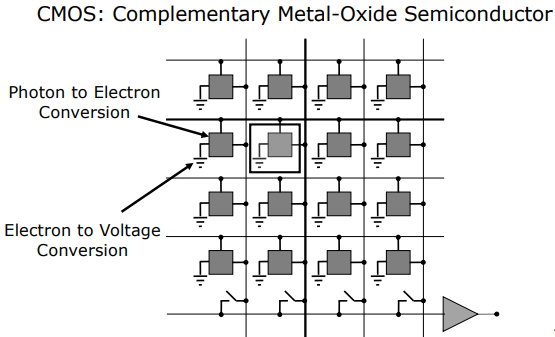
| Architecture Comparison | CCD (Charge-Coupled Device) | CMOS (Active-Pixel Sensor) |
|---|---|---|
| Charge Conversion | Off-pixel (Single corner amplifier) | On-pixel (Transistor in every pixel) |
| Readout Type | Serial charge transfer (“Bucket Brigade”) | Parallel voltage readout (Random access) |
| Power Consumption | High (Requires multi-phase high-voltage clocks) | Low (Standard CMOS digital voltage supply) |
| Readout Speed | Limited by serial transfer bottleneck | Extremely high (Column-parallel ADCs) |
| Fill Factor | $\approx 100%$ (No on-pixel transistors) | Reduced (Transistor circuitry occupies pixel area) |
3.5 Micro-Optics: The Microlens Array
To overcome the fill factor reduction caused by on-pixel transistor circuitry in CMOS sensors, semiconductor manufacturers integrate a Microlens Array above the sensor surface.
flowchart TD
L1["Incoming Light Rays from Main Camera Lens"] --> L2["Curved Organic Microlens Array"]
L2 -->|"Funnel Photon Cone"| L3["Color Filter Layer (Bayer RGB Dye)"]
L3 --> L4["Metal Interconnect & Wiring Layer (Opaque Circuit Tracks)"]
L4 -->|"Focus Light into Active Gap"| L5["Active Silicon Photodiode Window"]
style L1 fill:#1a1a2e,stroke:#888,color:#fff
style L2 fill:#16213e,stroke:#4cc9f0,color:#fff
style L3 fill:#0f3460,stroke:#f72585,color:#fff
style L4 fill:#e94560,stroke:#fff,color:#fff
style L5 fill:#06d6a0,stroke:#111,color:#000
- Operation: A curved organic micro-lenslet is fabricated directly over each pixel.
- Photon Funneling: Rather than allowing light rays to strike non-sensitive transistor metal tracks, the microlens collects photons across the entire pixel pitch area and refracts them directly onto the active photodiode area.
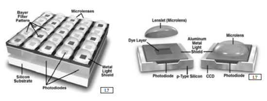
- Micro-Layer Stack: Scanning Electron Microscopy (SEM) reveals a micro-stack height of only $\approx 9.6\ \mu\text{m}$ from the top microlens apex to the silicon substrate:
- Top Layer: Curved organic microlens array
- Intermediate Layer: Color filter array (RGB dye)
- Base Layer: Silicon substrate with photodiode wells, floating diffusion, and metal interconnects.
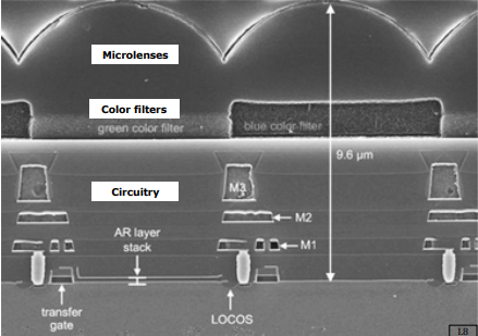
Resolution, Noise, Dynamic Range, and Color Sensing
- 1. Resolution, Noise, and Dynamic Range
- 2. Sensing Color
1. Resolution, Noise, and Dynamic Range
An image sensor’s performance is mathematically and physically constrained by its geometric resolution, electronic noise floor, and dynamic range limit. Understanding these parameters is essential for designing robust computer vision pipelines.
1.1 Resolution Trends
From the mid-1990s to the early 2010s, sensor resolution underwent rapid growth, shifting from sub-megapixel formats (typically $640 \times 480$ pixels) to standard consumer formats exceeding 16 megapixels. While early sensors suffered from high power draw and severe thermal limitations, modern semiconductor nodes produce low-power, high-density sensors with extremely low noise figures, often yielding resolutions (e.g., 50 megapixels) that exceed the requirements of standard computer vision applications.
Key Insight: Modern sensor manufacturing has largely decoupled pixel density from readout speed, shifting the primary bottleneck in computer vision from spatial resolution to data transmission bandwidth and real-time processing throughput.
1.2 Mathematical Formulations of Sensor Noise
Noise represents an unwanted modification of the optical signal introduced during its capture, electronic conversion, digital processing, transmission, or storage. Digital imaging systems suffer from five primary noise sources, categorized as scene-dependent or scene-independent:
flowchart TD
subgraph SceneDep ["Scene-Dependent Noise"]
N1["1. Photon Shot Noise<br/>(Poisson Distributed)"]
end
subgraph SceneIndep ["Scene-Independent Noise Floor"]
N2["2. Readout / Electronic Noise<br/>(Gaussian Distributed)"]
N3["3. Quantization Noise<br/>(Uniform ADC Rounding)"]
N4["4. Dark Current / Thermal Noise<br/>(Poisson Distributed)"]
N5["5. Fixed Pattern Noise (FPN)<br/>(Gain & Offset Variances)"]
end
TOTAL["Total Image Sensor Noise Floor"]
SceneDep --> TOTAL
SceneIndep --> TOTAL
style SceneDep fill:#1a1a2e,stroke:#e94560,color:#fff
style SceneIndep fill:#16213e,stroke:#4cc9f0,color:#fff
style TOTAL fill:#0f3460,stroke:#f72585,color:#fff
style N1 fill:#e94560,stroke:#fff,color:#fff
style N2 fill:#06d6a0,stroke:#111,color:#000
style N3 fill:#118ab2,stroke:#fff,color:#fff
style N4 fill:#7209b7,stroke:#fff,color:#fff
style N5 fill:#4361ee,stroke:#fff,color:#fff
1.2.1 Photon Shot Noise (Scene-Dependent)
Photon shot noise arises directly from the quantum and discrete nature of light. Light photons arrive at a pixel’s aperture randomly over time, analogous to raindrops falling into a bucket. This arrival sequence is modeled mathematically using the Poisson Distribution:
$$P(k) = \frac{\lambda^k e^{-\lambda}}{k!}$$
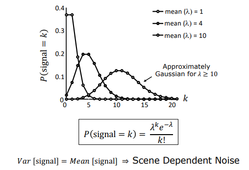
where:
- $\lambda$ is the expected average photon flux incident on the pixel during the integration period (representing true scene brightness).
- $k$ is the actual number of photons captured during a specific exposure window.
Mathematical Property
A fundamental property of the Poisson distribution is that its variance ($\sigma^2$) is equal to its mean ($\lambda$):
$$\text{Var}(\text{Signal}) = \sigma^2 = \lambda$$
$$\text{Standard Deviation } (\sigma) = \sqrt{\lambda}$$
Scene Dependence & SNR
Because variance is tied directly to true brightness $\lambda$, shot noise is heavily scene-dependent. Under high-intensity illumination (large $\lambda$), the absolute noise standard deviation increases, but the Signal-to-Noise Ratio (SNR) improves because the signal grows faster than the noise:
$$\text{SNR} = \frac{\text{Signal}}{\text{Noise}} = \frac{\lambda}{\sqrt{\lambda}} = \sqrt{\lambda}$$
Gaussian Convergence
For relatively bright regions where $\lambda \ge 10$, the Poisson distribution mathematically converges to a standard symmetric Gaussian curve.
1.2.2 Readout Noise (Scene-Independent)
Readout noise represents the electronic noise introduced during the physical conversion of accumulated photo-electrons into an analog voltage and its subsequent pre-amplification. It is modeled as an additive Gaussian Distribution:
$$P(x) = \frac{1}{\sigma \sqrt{2\pi}} \exp\left( -\frac{(x - \mu)^2}{2\sigma^2} \right)$$
where:
- $\mu$ is the true signal value (mean electron count converted to voltage).
- $\sigma$ is the standard deviation representing the thermal and electronic noise floor of the readout circuitry.
Quality Factor: High-quality scientific sensors feature a narrow Gaussian spread (low $\sigma$), whereas low-cost sensors exhibit a wide spread (high $\sigma$). Readout noise is entirely independent of scene brightness.
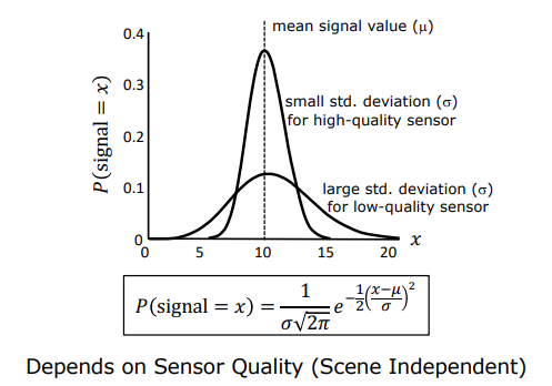
1.2.3 Quantization Noise (Scene-Independent)
Quantization noise occurs when continuous analog voltage is mapped to a discrete integer value during Analog-to-Digital Conversion (ADC).
If the quantization step (the voltage interval between two consecutive digital gray levels) is denoted as $\Delta$, the rounding error is uniformly distributed between $-\frac{\Delta}{2}$ and $+\frac{\Delta}{2}$.
Quantization Variance
The variance ($\sigma^2_q$) of this uniform error distribution is given by:
$$\sigma^2_q = \frac{\Delta^2}{12}$$
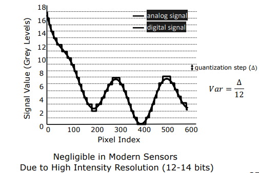
For modern high-performance sensors offering 12-bit to 14-bit intensity resolution, the step size $\Delta$ is extremely small, rendering quantization noise mathematically negligible.
1.2.4 Dark Current / Thermal Noise (Scene-Independent)
Even when the camera lens is covered by a light-tight lens cap, thermal energy within the silicon substrate excites valence electrons into the conduction band, accumulating spurious charge in the potential wells.
- Characteristics: This thermally generated dark current follows a Poisson distribution and accumulates linearly over integration time.
- Relevance: It is negligible in standard consumer photography due to short exposure times. However, in scientific applications requiring long integrations (e.g., astronomy or extreme low-light imaging), dark current accumulates rapidly, drowning out dim optical signals.
- Mitigation: To suppress dark current, scientific cameras are cooled to cryogenic temperatures using liquid nitrogen or thermoelectric Peltier coolers.
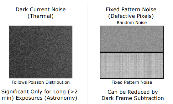
1.2.5 Fixed Pattern Noise (Scene-Independent)
Fixed Pattern Noise (FPN) refers to spatial variations in pixel responses under completely uniform illumination.
- Origin: It is caused by unavoidable manufacturing tolerances that result in microscopic differences in potential well capacities, photo-site geometries, and pixel-level amplifier gains.
- Mitigation: Unlike random electronic noise, FPN is static over time. It can be calibrated out by capturing a flat-field frame (a uniform grey image), calculating a localized scale-and-offset correction factor for each pixel, and applying these gain factors to all subsequent captured frames.
1.3 Dynamic Range (DR)
Dynamic range defines the sensor’s capacity to measure extreme contrast variations within a single scene. It is mathematically defined as:
$$\text{DR} = 20 \log_{10} \left( \frac{b_{\max}}{b_{\min}} \right)\ \text{dB}$$
where:
- $b_{\max}$ is the Full-Well Capacity (saturation limit) of the pixel, representing the maximum number of electrons the potential well can hold before saturating. Any additional photons striking a saturated pixel overflow into neighboring pixels (blooming) and do not increase the output value.
- $b_{\min}$ is the Minimum Detectable Photon Energy, determined by the noise floor of the system. If the signal amplitude is lower than the standard deviation of the noise ($\text{Signal} < \sigma_{\text{Noise}}$), the optical signal is mathematically indistinguishable from noise.
Comparative Dynamic Range Performance
| Imaging System | Dynamic Range Ratio | Dynamic Range (dB) |
|---|---|---|
| Human Eye | 1,000,000 : 1 | 120 dB |
| High Dynamic Range (HDR) Display | 200,000 : 1 | 106 dB |
| Consumer Digital Camera (Still) | 4,096 : 1 | 72.2 dB |
| Standard Photographic Film | 2,948 : 1 | 66.2 dB |
| Standard Digital Video Camera | 45 : 1 | 33.1 dB |
Video Limitation: Digital video sensors suffer from heavily compressed dynamic ranges. To maintain standard frame rates (e.g., 30 fps), the maximum integration (exposure) time is limited to a fraction of a second (e.g., $30\text{ ms}$). This brief exposure limits total accumulated photon energy ($b_{\max}$ cannot be reached for mid-tones), reducing the overall SNR while electronic readout noise remains constant.
2. Sensing Color
Color is not a physical property of light; rather, it is a human psycho-physical and neuro-chemical response to specific electromagnetic wavelengths.
2.1 The Mathematics of Spectral Integration
When an incoming light wave carrying a continuous spectral photon distribution $p(\lambda)$ strikes a silicon photodiode, the sensor collapses this continuous spectral curve into a single scalar value representing electron flux.
Quantum Efficiency of Silicon ($q(\lambda)$)
The ratio of generated electron flux to incident photon flux as a function of wavelength ($\lambda$) defines silicon’s quantum efficiency ($q(\lambda)$):
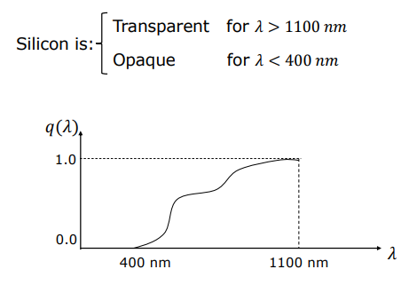
The Integration Equation
For a pixel under continuous illumination from a light source with spectral distribution $p(\lambda)$, the total generated electron flux $I$ is mathematically represented as:
$$I = \int_{0}^{\infty} q(\lambda) p(\lambda) , d\lambda$$
Information Loss: Because $I$ is a single integrated scalar value, it is mathematically impossible to reconstruct the multi-dimensional spectral curve $p(\lambda)$ from $I$ alone. An infinite variety of distinct spectral curves can yield the exact same scalar value $I$.
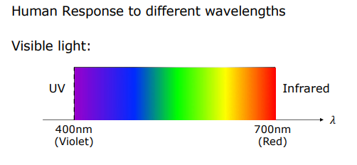
2.2 Reconstructing the Spectrum via Filter Sifting
To reconstruct the spectral curve $p(\lambda)$, optical filters are integrated in front of the pixel array, with each filter $i$ featuring a spectral response function $f_i(\lambda)$.
flowchart TD
P["Incoming Spectral Distribution p(λ)"] --> F["Optical Filter Response f_i(λ)<br/>(Delta Function δ(λ - λ_i))"]
F --> I["Sifted Scalar Value:<br/>I_i = q(λ_i) · p(λ_i)"]
style P fill:#1a1a2e,stroke:#4cc9f0,color:#fff
style F fill:#16213e,stroke:#e94560,color:#fff
style I fill:#0f3460,stroke:#06d6a0,color:#fff
If we utilize a set of highly idealized, narrow-band filters modeled mathematically as Dirac Delta functions centered at specific wavelengths $\lambda_i$:
$$f_i(\lambda) = \delta(\lambda - \lambda_i)$$
The resulting electron flux equation simplifies due to the sifting property of the Delta function:
$$I_i = \int_{0}^{\infty} q(\lambda) p(\lambda) \delta(\lambda - \lambda_i) , d\lambda = q(\lambda_i) p(\lambda_i)$$
- Spectrum Reconstruction: By measuring $I_i$ across multiple discrete filter wavelengths $\lambda_i$, we can extract individual points along the spectral curve $p(\lambda)$.
- Finite Filters: While full spectral reconstruction theoretically requires infinite filters, because physical spectral distributions $p(\lambda)$ in nature are smooth and lack high-frequency variations, a small, finite set of filters is mathematically sufficient to reconstruct the spectrum without loss of information.
2.3 Biological Vision: Rods and Cones
The human visual system utilizes the same integration and filtering principles to perceive color.
The Retina Architecture
The retina is a curved biological image sensor with a counter-intuitive backwards physical structure:
- Light enters the eye, passes through the lens, and strikes the front-most layers of the retina containing ganglion cells and bipolar cells.
- Light must travel through these semi-transparent neural layers before finally reaching the light-sensitive photoreceptors (rods and cones) anchored at the very back of the retina.
flowchart TD
LIGHT["Direction of Incoming Light Rays"] --> L1["1. Ganglion Cells Layer<br/>(Early Signal Processing)"]
L1 --> L2["2. Bipolar Cells Layer<br/>(Neural Transmission)"]
L2 --> L3["3. Photoreceptors Layer (Rods & Cones)<br/>(Light-Sensitive Layer at the BACK of Retina)"]
style LIGHT fill:#1a1a2e,stroke:#fff,color:#fff
style L1 fill:#16213e,stroke:#4cc9f0,color:#fff
style L2 fill:#0f3460,stroke:#f72585,color:#fff
style L3 fill:#e94560,stroke:#06d6a0,color:#fff
Rods vs. Cones
Rods (Scotopic Vision)
- Quantity: Approximately 120 million per retina.
- Protein: Contains the light-sensitive protein rhodopsin.
- Function: Highly sensitive to low photon densities, enabling monochromatic nighttime vision. Rods do not perceive color, which explains why scenes observed under dim moonlight appear gray and desaturated.
Cones (Photopic Vision)
- Quantity: Approximately 7 million per retina.
- Protein: Contains the protein photopsin.
- Function: Requires high photon densities to trigger, enabling sharp, full-color daylight vision.
- Spatial Distribution: Cones are highly concentrated at the fovea, the central point of the retina responsible for high-acuity vision. Conversely, rods are completely absent in the center of the fovea, peaking in density in peripheral regions.
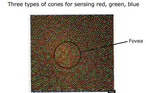
2.4 Tristimulus Values and Metamers
Humans are trichromats, possessing three distinct types of cone cells (often simplified as Red, Green, and Blue cones). Their respective spectral response curves are known as tristimulus curves:
- $h_R(\lambda)$ (L-cones, sensitive to long wavelengths)
- $h_G(\lambda)$ (M-cones, sensitive to medium wavelengths)
- $h_B(\lambda)$ (S-cones, sensitive to short wavelengths)
Tristimulus Integration Equations
For any incident spectral light distribution $p(\lambda)$, the retina collapses this spectrum into exactly three scalar values, known as the tristimulus values ($R, G, B$):
$$R = \int_{0}^{\infty} h_R(\lambda) p(\lambda) , d\lambda$$
$$G = \int_{0}^{\infty} h_G(\lambda) p(\lambda) , d\lambda$$
$$B = \int_{0}^{\infty} h_B(\lambda) p(\lambda) , d\lambda$$
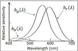
The Metamerism Phenomenon
Because the human brain receives only these three integrated scalar values ($R, G, B$), it cannot reconstruct the original continuous spectrum $p(\lambda)$. This leads to the phenomenon of metamerism:
- Definition: Metamers are physically distinct spectral distributions $p_1(\lambda) \neq p_2(\lambda)$ that yield identical tristimulus values ($R_1 = R_2, G_1 = G_2, B_1 = B_2$) when integrated against human tristimulus curves.
- Result: Even though the physical light waves are completely different, humans perceive them as the exact same color. For example, multiple distinct spectral distributions can yield the same tristimulus values of $R=115, G=60, B=108$, which the brain perceives as a single unified shade of purple or magenta.
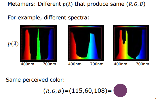
2.5 Young’s Color Mixing and Camera Filtering
In his seminal color mixture experiment, Thomas Young demonstrated that projecting and mixing just three primary wavelengths of light (650 nm (red), 530 nm (green), and 410 nm (blue)) in varying intensities can reproduce almost the entire gamut of colors perceivable by humans. This fundamental tri-chromatic discovery enables modern cameras and displays to use only three filters to capture and reproduce natural scenes.
Digital Color Capture Architectures
Dichroic Prism (3-CCD System)
- Mechanism: A complex glass prism splits the incoming image into red, green, and blue spectral components using internal interference coatings. Three independent, perfectly aligned image sensors are mounted on the faces of the prism to simultaneously record $R$, $G$, and $B$ channels at every pixel coordinate.
- Evaluation: This system produces ultra-high-fidelity color maps with no spatial aliasing, but is extremely bulky, expensive, and structurally fragile.
flowchart LR
IN["Incoming Light Ray"] --> PRISM["Dichroic Prism Splitter"]
PRISM -->|"Red Wavelengths"| SR["Sensor 1: Red Channel"]
PRISM -->|"Green Wavelengths"| SG["Sensor 2: Green Channel"]
PRISM -->|"Blue Wavelengths"| SB["Sensor 3: Blue Channel"]
style IN fill:#1a1a2e,stroke:#fff,color:#fff
style PRISM fill:#16213e,stroke:#4cc9f0,color:#fff
style SR fill:#e94560,stroke:#fff,color:#fff
style SG fill:#06d6a0,stroke:#fff,color:#000
style SB fill:#118ab2,stroke:#fff,color:#fff
Color Filter Mosaic (Bayer Pattern)
- Mechanism: A single CMOS sensor is coated with a repeating $2\times2$ grid of color filters, commonly the Bayer Pattern (consisting of $50%$ Green, $25%$ Red, and $25%$ Blue filters). Green filters dominate because human vision is most sensitive to green wavelengths.
- Raw Image: Each pixel captures only a single color component ($R$, $G$, or $B$), resulting in a mosaiced “raw” image.
- Demosaicing: To reconstruct a full-color image where every pixel possesses complete $R, G, B$ values, an interpolation algorithm (demosaicing) analyzes neighboring pixel values to estimate missing color channels.
Camera Response, HDR Imaging, and Nature’s Sensors
- 1. Camera Response Function and Radiometric Calibration
- 2. High Dynamic Range (HDR) Imaging
- 3. Nature’s Image Sensors and Biological Vision
1. Camera Response Function and Radiometric Calibration
While the relationship between the physical photon flux and the generated sensor charge is highly linear, consumer cameras output non-linear pixel intensities.
1.1 The Camera Response Function ($f$)
When light strikes a sensor pixel, the relationship between scene brightness and measured image intensity is guaranteed to be monotonic, but is rarely linear.
flowchart LR
FLUX["Incoming Photon Flux (I)"] --> EXP["Pixel Linear Charge (B)<br/>B = I · e = I · (A · T)"]
EXP --> ISP["Electronics & Image Signal Processor (ISP)<br/>(ADC, Demosaicing, Sharpening)"]
ISP --> OUT["Non-Linear Output Intensity (M)<br/>M = f(B)"]
style FLUX fill:#1a1a2e,stroke:#fff,color:#fff
style EXP fill:#16213e,stroke:#4cc9f0,color:#fff
style ISP fill:#0f3460,stroke:#f72585,color:#fff
style OUT fill:#e94560,stroke:#06d6a0,color:#fff
Linear Exposure ($B$)
The raw intensity $B$ inside the pixel is strictly linear with respect to the incoming photon flux $I$ and the total exposure $e$. Exposure is the product of the aperture area $A$ (related to diameter $D$) and the integration time $T$:
$$B = I \times e = I \times (A \times T)$$
Electronic Modulation
Before being outputted as a digital measurement $M$, this linear charge $B$ undergoes electron-to-voltage conversion, Analog-to-Digital conversion (ADC), and several digital image signal processing (ISP) operations (such as demosaicing, sharpening, and contrast enhancement).
Non-Linear Squeezing (Gamma Curve)
Camera manufacturers intentionally introduce a non-linear mapping function $f$ (known as the Gamma Curve or Gamma Function):
$$M = f(B)$$
The Squeezing Principle: Because digital image formats have a finite dynamic range (typically 8 bits per channel, 0 to 255), mapping linear intensities directly would waste precious numerical bits on bright highlights that the human eye cannot easily distinguish. Instead, $f$ compresses the bright, high-intensity regions (like clouds in the sky) while dedicating much higher numerical resolution to darker values, preserving critical shadow details.
1.2 Radiometric Calibration
For many quantitative computer vision applications (such as photometric stereo or shape from shading), the true linear scene irradiance must be recovered from the non-linear pixel values $M$. The process of finding and inverting this non-linear function $f$ is called radiometric calibration.
flowchart TD
MAB["Standard Macbeth Color Chart<br/>(Neutral Gray Patches: 3.1% to 90.0% Reflectance)"] --> ILL["Uniform Distant Illumination<br/>(Linear Brightness B ∝ Reflectance)"]
ILL --> CAP["Capture Single Test Frame<br/>(Normalize Peak Patch to 1.0)"]
CAP --> CURVE["Plot Reflectance (B) vs Digital Intensity (M)<br/>(Reconstruct Response Function f)"]
CURVE --> INV["Apply Inverse Response Function f⁻¹(M)<br/>(Recover True Linear Scene Irradiance B)"]
style MAB fill:#1a1a2e,stroke:#4cc9f0,color:#fff
style ILL fill:#16213e,stroke:#e94560,color:#fff
style CAP fill:#0f3460,stroke:#f72585,color:#fff
style CURVE fill:#e94560,stroke:#fff,color:#fff
style INV fill:#06d6a0,stroke:#111,color:#000
Calibration Steps Using a Macbeth Chart
- Chart Selection: A standard Macbeth Chart contains a bottom row of neutral gray patches with precisely known physical reflectance values, spanning from 3.1% (dark patch) to 90.0% (bright patch).
- Uniform Illumination: The chart is illuminated using distant light sources, ensuring a perfectly uniform illumination over the entire surface.
- Reflectance Proportionality: Because illumination is constant, the true linear image brightness $B$ of each gray patch is directly proportional to its known physical reflectance, scaled by an unknown constant factor $k$ (which depends on light source intensity, camera gain, etc.): $$B \propto \text{Reflectance}$$
- Plotting and Inversion: A single image of the chart is captured. The brightest patch’s linear intensity is normalized to 1.0 to eliminate the unknown scale factor $k$.
- Curve Reconstruction: By plotting the known linear reflectances on the x-axis ($B$) and the measured digital pixel values on the y-axis ($M$), we reconstruct the camera’s response curve $f$.
Once $f$ is calibrated, we can linearize any subsequent image captured by the camera by passing the pixels through the inverse function $f^{-1}$, recovering true scene brightness up to a single scale factor:
$$B = f^{-1}(M)$$
2. High Dynamic Range (HDR) Imaging
Real-world environments exhibit an enormous range of light intensities that far exceed the 72 dB dynamic range of consumer sensors.
2.1 Exposure Bracketing
Exposure bracketing combines multiple frames of a static scene captured at different integration times to synthesize an image with a wider dynamic range.
flowchart TD
subgraph Bracket ["Multi-Exposure Sequence"]
E0["Frame M0 (Short Exposure e0)<br/>Captures Highlights (Window / Sky)"]
E1["Frame M1 (Medium Exposure e1)<br/>Captures Mid-Tones"]
E2["Frame M2 (Long Exposure e2)<br/>Captures Shadows"]
E3["Frame M3 (Ultra Exposure e3)<br/>Captures Darkest Indoor Details"]
end
Bracket --> SUM["Linear Addition (Linearized Images)<br/>M_HDR = M0 + M1 + M2 + M3"]
SUM --> TONE["Tone Mapping Algorithm<br/>(Compresses 10-bit / 1020 Range to 8-bit)"]
TONE --> OUT["Final HDR Image<br/>(Full Detail in Highlights & Shadows)"]
style Bracket fill:#1a1a2e,stroke:#4cc9f0,color:#fff
style SUM fill:#16213e,stroke:#e94560,color:#fff
style TONE fill:#0f3460,stroke:#f72585,color:#fff
style OUT fill:#06d6a0,stroke:#111,color:#000
Multi-Exposure Sequence
The camera captures a sequence of pictures with varying exposure times $e_0 < e_1 < e_2 < e_3$.
Mathematical Slices
For a scene point with true brightness $P$, the measured value in frame $i$ is capped at the sensor’s maximum saturation limit of 255:
$$M_i = \min(e_i \cdot P,\ 255)$$
- Short Exposure ($e_0$): Prevents highlights (such as a bright sky or window) from saturating, but leaves shadows completely black and noisy.
- Long Exposure ($e_3$): Floods the sensor with photons, capturing details in dark indoor shadows, but completely washes out and saturates outdoor regions.
Linear Addition
Assuming the camera response has been linearized ($f^{-1}$ applied), we sum these four exposures to generate an aggregate image:
$$M_{\text{HDR}} = M_0 + M_1 + M_2 + M_3$$
The combined response function of this aggregate virtual camera compresses high scene intensities while maintaining high sensitivity in dark regions, yielding a maximum numerical value of 1020 ($4 \times 255$).
Tone Mapping
A tone mapping algorithm compresses this high-fidelity 10-bit output back down to standard 8-bit display formats, rendering both indoor shadows and outdoor skies with rich detail.
The Ghosting Artifact: Exposure bracketing works exceptionally well for static scenes but fails in dynamic environments. If an object (such as a bicyclist or pedestrian) moves during the multi-exposure capture sequence, it is recorded at different spatial coordinates in each frame. Adding these frames results in semi-transparent, duplicated overlapping copies in the final image, known as ghosting.
2.2 Single-Shot HDR via Assorted Pixels
To capture HDR images of moving objects without ghosting, the entire dynamic range must be recorded in a single exposure. This is achieved using spatially varying pixel exposures (SVE), commonly referred to as Assorted Pixels.
- Pixel-Level Sensitivity Modulation: Instead of a uniform sensor where all pixels have identical sensitivity, an assorted pixel sensor features adjacent photodiodes with unequal light sensitivities.
- Optomechanical Implementation: This spatial variation is implemented by depositing micro-shades of varying optical transparencies directly over adjacent pixels or driving neighboring pixels with different integration times.
- Spatial Interpolation Pipeline:
- If a highly sensitive pixel saturates (clips to 255) under bright light, its less-sensitive (shaded) neighbor will not saturate and will successfully record the highlight detail.
- If a shaded pixel is too dark, its unshaded neighbor will capture clean, high-SNR details in the shadows.
- An interpolation algorithm then processes this patterned checkerboard image, predicting missing high-exposure and low-exposure values from neighboring pixels.
- Result: This single-shot HDR architecture produces full-color, high-contrast images with no motion artifacts and is widely used in modern smartphone camera modules.
3. Nature’s Image Sensors and Biological Vision
Over millions of years of evolution, nature has engineered visual systems that solve complex sensing challenges with elegant, non-traditional configurations.
3.1 Copilia’s Mechanical Scanning Eye
The marine crustacean Copilia (a microscopic plankton-like creature) possesses an eye that operates as an optomechanical scanner.
flowchart TD
L1["Anterior Lens (Large Outer Lens)<br/>Fixed Focus to Internal Image Plane"] --> PLANE["Internal Image Plane<br/>(2D Optical Projection)"]
PLANE --> L2["Mobile Posterior Lens + Single Biological Photoreceptor<br/>(Mechanically Scanned Back and Forth)"]
L2 --> BRAIN["Copilia Brain<br/>(Reconstructs 2D Visual Field Over Time)"]
style L1 fill:#1a1a2e,stroke:#4cc9f0,color:#fff
style PLANE fill:#16213e,stroke:#e94560,color:#fff
style L2 fill:#0f3460,stroke:#f72585,color:#fff
style BRAIN fill:#06d6a0,stroke:#111,color:#000
- Optics: Each eye contains two lenses. A large, static outer anterior lens focuses light to form a two-dimensional image inside the head.
- Mechanical Scanning: Positioned behind this image plane is a mobile posterior lens paired with a single biological photoreceptor (a single-pixel sensor).
- Operation: Instead of utilizing a dense grid of millions of receptors, Copilia mechanically scans this posterior lens-receptor assembly back and forth across the anterior lens’s focal plane. By scanning the single pixel spatially over time, Copilia’s brain reconstructs a complete two-dimensional image of its environment.
3.2 Brittle Star (Ophiocoma wendtii): The Lens-Covered Body
The Brittle Star (yılan yıldızı) is a marine creature with no brain and no traditional focal eyes. For decades, biologists were puzzled by its ability to navigate complex crevices and evade predators.
- The Discovery: Around 2001, scanning electron microscopy revealed that the entire calcitic skeletal body of the brittle star is covered with millions of tiny, highly transparent calcite crystal bumps.
- Optical Precision: Each crystal bump is an optically perfect microlens, measuring approximately 1/20 of a millimeter in diameter.
- The Flexible Camera: These calcitic microlenses focus light onto a bundle of nerve fibers running directly underneath them. The brittle star’s entire skeletal body effectively functions as a massive, flexible, curved image sensor, allowing it to perceive spatial distributions of light and shadow across its entire body.
3.3 Octopus Camouflage and Chromatophores
The skin of the octopus is a dynamic biological display and sensor array.
- Chromatophores: The skin contains millions of microscopic pigment-filled sacs called chromatophores.
- Neural Control: These sacs are directly controlled by surrounding muscle fibers. When the brain sends a neural impulse, the muscles contract or expand, changing the physical shape and surface area of the pigment sacs.
- Camouflage: By precisely modulating which colors are exposed, the octopus can match the texture, color, and reflectance of surrounding coral reefs or plants. This real-time camouflage is so perfect that the octopus remains completely invisible to predators even at close distances.
3.4 The Human Eye Blind Spot
In the human eye, the biological wiring of the retina creates a unique optical defect.
- The Optic Disk: All nerve impulses generated by the rods and cones travel along axons that gather at a single point on the retina: the optic disk.
- Zero Receptor Density: At this exit point, the optic nerve passes through the retinal layer to travel to the visual cortex of the brain. Because the nerve occupies this space, there is a physical patch on the retina that is completely devoid of rods and cones. This is the blind spot.
Neural Inpainting: We do not notice a physical hole in our daily field of view because our brain performs real-time spatial “inpainting” (interpolation), filling in missing visual information based on surrounding texture, color, and context.
Mathematical Foundations and Geometric Properties of Binary Images
- 1. The Nature and Acquisition of Binary Images
- 2. Geometric Moments and Position Estimation in Continuous Binary Images
- 3. Determining Object Orientation (Axis of Least Second Moment)
- 4. Solving Orientation Angle and Shape Analysis
- 5. Discrete Binary Images and Real-Time Hardware Computation
Binary images represent the simplest yet most robust and computationally efficient image representation in computer vision, particularly within industrial automation and structured environments. This section explores the physical and mathematical processes involved in converting grayscale images into binary representations, alongside the continuous and discrete geometric moment calculations used to determine the position, orientation, and structural properties of single objects.
Key Insight: Binary images eliminate complex color and texture details to focus exclusively on object geometry. Through appropriate optical setup and moment analysis, an object’s position ($x, y$), area ($A$), and orientation ($\theta$) can be computed with $O(N)$ complexity in milliseconds.
1. The Nature and Acquisition of Binary Images
A binary image is a matrix structure where each pixel takes one of only two possible values ($0$ or $1$). Typically, a value of $1$ (white) denotes the foreground object under analysis, while $0$ (black) represents the background.
1.1 Thresholding and the Characteristic Function
The mathematical transformation used to convert a grayscale image $g(x,y)$ into a binary image $b(x,y)$ is called thresholding. This operation is defined by the characteristic (indicator) function:
$$b(x,y) = \begin{cases} 0, & g(x,y) < T \ 1, & g(x,y) \ge T \end{cases}$$
Here, $T$ denotes the global threshold value defining the intensity boundary.
flowchart LR
A["Grayscale Image<br/>g(x, y)"] --> B{"Threshold Check<br/>g(x, y) ≥ T?"}
B -->|Yes| C["Foreground (1)"]
B -->|No| D["Background (0)"]
style A fill:#1a1a2e,stroke:#e94560,color:#fff
style B fill:#16213e,stroke:#4cc9f0,color:#fff
style C fill:#0f3460,stroke:#06d6a0,color:#fff
style D fill:#2b2d42,stroke:#8d99ae,color:#fff
1.2 Selection of Optimum Threshold Value (Histogram Valley)
To automatically determine an optimal threshold $T$, the brightness histogram of the grayscale image is analyzed. In controlled lighting environments, the histogram typically exhibits a bimodal distribution:
- First Mode (Peak): Corresponding to the concentration of background pixels.
- Second Mode (Peak): Corresponding to the concentration of foreground object pixels.
The deepest point between these two peaks is called the valley. Selecting the ideal threshold $T$ at this valley intensity provides the most stable separation of object boundaries.
1.3 Stable Configurations and Silhouette Imaging
Three-dimensional objects resting on a planar surface assume a finite number of stable configurations under gravity. A overhead camera observes the object in one of these stable resting poses (subject to 2D translation and rotation). This property allows 3D objects to be identified and localized via 2D binary silhouette analysis.
However, under direct top-down illumination, shadows, specularities, surface textures, and material reflectance often cause simple thresholding to fail. To overcome these physical limitations, a Backlighting optical arrangement is employed:
- Objects are placed on a translucent surface illuminated uniformly from below.
- When viewed from above, the object completely blocks the light, delivering a high-contrast, smooth, and noise-free silhouette directly to the camera sensor.
flowchart TD
A["Uniform Light Source (Below)"] --> B["Translucent Diffuser Surface"]
B --> C["Object (Blocks Light)"]
C --> D["Overhead Camera"]
D --> E["High-Contrast Silhouette Image b(x,y)"]
style A fill:#1a1a2e,stroke:#e94560,color:#fff
style B fill:#16213e,stroke:#4cc9f0,color:#fff
style C fill:#0f3460,stroke:#f72585,color:#fff
style D fill:#1a1a2e,stroke:#06d6a0,color:#fff
style E fill:#2b2d42,stroke:#8d99ae,color:#fff
Key Insight: Backlighting leverages optical physics rather than heavy software preprocessing to generate flawless binary silhouettes directly at the sensor level.
2. Geometric Moments and Position Estimation in Continuous Binary Images
Geometric properties are analyzed under the assumption that a single object is present in continuous space. The characteristic function takes $b(x,y) = 1$ over the object domain and $b(x,y) = 0$ over the background.
2.1 Area (Zero-th Moment)
The total area ($A$) occupied by the object represents the zeroth moment of the image, calculated by integrating over the image domain:
$$A = \iint b(x,y) , dx , dy$$
Area is the most fundamental invariant feature for distinguishing among a finite set of known objects regardless of translation or rotation.
2.2 Position (Center of Area / Centroid - First Moment)
The object’s position in the image plane is defined by its center of area (centroid). This center directly corresponds to the center of mass of a thin planar plate with uniform density. Dividing the first moments by the total area yields the centroid coordinates $(\bar{x}, \bar{y})$:
$$\bar{x} = \frac{1}{A} \iint x \cdot b(x,y) , dx , dy$$
$$\bar{y} = \frac{1}{A} \iint y \cdot b(x,y) , dx , dy$$
3. Determining Object Orientation (Axis of Least Second Moment)
For a robotic arm to grasp an object accurately, it requires both the centroid position and the planar orientation of the object. Orientation is defined mathematically by the Axis of Least Second Moment.
3.1 Second Moment Function ($E$) and Line Parameterization
The second moment ($E$) about any axis is the integral of the squared perpendicular distances ($r$) from all object points to that axis:
$$E = \iint r^2 \cdot b(x,y) , dx , dy$$
The standard line equation $y = mx + b$ introduces singularity errors in optimization as vertical lines approach $m \to \infty$. Therefore, a trigonometric line parameterization is used:
$$x \sin\theta - y \cos\theta + \rho = 0$$
Where:
- $\theta$: The angle between the normal to the line and the horizontal axis ($\theta \in [0, 2\pi]$).
- $\rho$: The perpendicular distance from the origin to the line.
The perpendicular distance $r$ from point $(x,y)$ to this line simplifies directly using $\sin^2\theta + \cos^2\theta = 1$:
$$r = x \sin\theta - y \cos\theta + \rho$$
3.2 Proof That the Axis Passes Through the Center of Area
Expanding the second moment expression yields:
$$E(\theta, \rho) = \iint (x \sin\theta - y \cos\theta + \rho)^2 \cdot b(x,y) , dx , dy$$
To find the value of $\rho$ that minimizes $E$, we set the partial derivative with respect to $\rho$ to zero:
$$\frac{\partial E}{\partial \rho} = 2 \iint (x \sin\theta - y \cos\theta + \rho) \cdot b(x,y) , dx , dy = 0$$
Distributing the integral and substituting the zeroth and first moment definitions ($A, \bar{x}, \bar{y}$):
$$\sin\theta \iint x \cdot b(x,y) , dx , dy - \cos\theta \iint y \cdot b(x,y) , dx , dy + \rho \iint b(x,y) , dx , dy = 0$$
$$A \bar{x} \sin\theta - A \bar{y} \cos\theta + A \rho = 0$$
Since $A \neq 0$, dividing by $A$ gives:
$$\bar{x} \sin\theta - \bar{y} \cos\theta + \rho = 0$$
Mathematical Proof: This equation confirms that the axis of least second moment must pass through the object’s center of area $(\bar{x}, \bar{y})$.
3.3 Eliminating $\rho$ via Coordinate Translation
Given that the axis passes through the centroid, we translate the origin to $(\bar{x}, \bar{y})$:
$$x’ = x - \bar{x} \quad \text{and} \quad y’ = y - \bar{y}$$
In this translated coordinate system, $\rho = 0$, reducing the second moment to:
$$E(\theta) = a \sin^2\theta - b \sin\theta \cos\theta + c \cos^2\theta$$
Where $a, b, c$ are the central second moments of the image:
- $a = \iint (x’)^2 \cdot b(x,y) , dx’ , dy’$ (moment of inertia about the $y$-axis)
- $b = 2 \iint (x’ y’) \cdot b(x,y) , dx’ , dy’$ (product / correlation moment)
- $c = \iint (y’)^2 \cdot b(x,y) , dx’ , dy’$ (moment of inertia about the $x$-axis)
4. Solving Orientation Angle and Shape Analysis
4.1 Orientation Angle Formula ($\theta$)
Differentiating $E(\theta)$ with respect to $\theta$ and setting it to zero yields:
$$\frac{\partial E}{\partial \theta} = 2a \sin\theta \cos\theta - b(\cos^2\theta - \sin^2\theta) - 2c \sin\theta \cos\theta = 0$$
Applying double-angle identities ($\sin 2\theta = 2\sin\theta\cos\theta$ and $\cos 2\theta = \cos^2\theta - \sin^2\theta$):
$$(a - c) \sin 2\theta - b \cos 2\theta = 0$$
Which gives the fundamental orientation equation:
$$\tan 2\theta = \frac{b}{a - c}$$
flowchart TD
A["Central Second Moments (a, b, c)"] --> B["Differentiate: ∂E/∂θ = 0"]
B --> C["Double-Angle Identity: (a-c)sin(2θ) - b cos(2θ) = 0"]
C --> D["Fundamental Equation: tan(2θ) = b / (a - c)"]
D --> E["Dual Solutions: θ_1 and θ_2 = θ_1 + π/2"]
E --> F{"Second Derivative Test<br/>∂²E/∂θ² > 0?"}
F -->|Yes| G["E_min Angle (True Orientation θ)"]
F -->|No| H["E_max Angle (Orthogonal Axis)"]
style A fill:#1a1a2e,stroke:#e94560,color:#fff
style B fill:#16213e,stroke:#4cc9f0,color:#fff
style C fill:#0f3460,stroke:#f72585,color:#fff
style D fill:#1a1a2e,stroke:#06d6a0,color:#fff
style E fill:#2b2d42,stroke:#8d99ae,color:#fff
style G fill:#06d6a0,stroke:#fff,color:#000
style H fill:#e94560,stroke:#fff,color:#fff
4.2 Dual Solution Geometry and Second Derivative Test
Due to the identity $\tan 2\theta = \tan(2\theta + \pi)$, there are two orthogonal solutions in $[0, 2\pi]$:
$$\theta_1 = \frac{1}{2} \text{atan2}(b, a-c)$$ $$\theta_2 = \theta_1 + \frac{\pi}{2}$$
One solution minimizes the second moment ($E_{min}$), while the other maximizes it ($E_{max}$). The second derivative test distinguishes the minimum:
$$\frac{\partial^2 E}{\partial \theta^2} = 2(a - c) \cos 2\theta + 2b \sin 2\theta$$
- If $\frac{\partial^2 E}{\partial \theta^2} > 0$, the angle $\theta$ minimizes $E$ ($E_{min}$).
- If $\frac{\partial^2 E}{\partial \theta^2} < 0$, the angle $\theta$ maximizes $E$ ($E_{max}$).
4.3 Roundedness Measure
To quantify whether an object is circular or elongated, the ratio of minimum to maximum second moment is evaluated:
$$\text{Roundedness} = \frac{E_{min}}{E_{max}}$$
This ratio ranges in $$:
- Elongated Objects: $E_{min} \ll E_{max}$, causing the ratio to approach $0$.
- Perfect Disk / Circle: Every axis passing through the centroid has identical moments of inertia ($a=c, b=0$). The roundedness ratio is exactly $1.0$.
5. Discrete Binary Images and Real-Time Hardware Computation
In digital systems, images consist of discrete pixels, where $b_{ij} \in {0, 1}$ represents the pixel value at row $i$ and column $j$.
5.1 Discrete Moment Formulas
-
Area (Zero-th Moment): $$A = \sum_{i} \sum_{j} b_{ij}$$
-
Center of Area (First Moment): $$\bar{x} = \frac{1}{A} \sum_{i} \sum_{j} j \cdot b_{ij} \quad \text{and} \quad \bar{y} = \frac{1}{A} \sum_{i} \sum_{j} i \cdot b_{ij}$$
5.2 Real-Time Hardware Calculation Strategy
During pixel streaming from a sensor, the centroid $(\bar{x}, \bar{y})$ is not yet known. Calculating moments directly relative to the centroid would require storing the full frame and making a second pass over memory, introducing latency.
To solve this, intermediate moments ($a’, b’, c’$) are accumulated relative to the top-left origin during streaming:
$$a’ = \sum_{i} \sum_{j} j^2 \cdot b_{ij}$$ $$b’ = 2 \sum_{i} \sum_{j} i \cdot j \cdot b_{ij}$$ $$c’ = \sum_{i} \sum_{j} i^2 \cdot b_{ij}$$
These intermediate accumulators ($a’, b’, c’$), area $A$, and first-order sums ($\sum j \cdot b_{ij}, \sum i \cdot b_{ij}$) are updated on-the-fly in hardware during a single pixel pass.
flowchart LR
A["Pixel Stream<br/>(i, j, b_ij)"] --> B["Single-Pass Hardware Accumulators:<br/>A, ∑j·b, ∑i·b, a', b', c'"]
B --> C["End of Frame Signal"]
C --> D["Algebraic Shift:<br/>a = a' - A·x̄²<br/>b = b' - 2A·x̄·ȳ<br/>c = c' - A·ȳ²"]
D --> E["Millisecond Outputs:<br/>Centroid (x̄, ȳ), Orientation (θ),<br/>and Roundedness"]
style A fill:#1a1a2e,stroke:#e94560,color:#fff
style B fill:#16213e,stroke:#4cc9f0,color:#fff
style C fill:#0f3460,stroke:#f72585,color:#fff
style D fill:#1a1a2e,stroke:#06d6a0,color:#fff
style E fill:#2b2d42,stroke:#8d99ae,color:#fff
Once frame readout finishes, the central second moments ($a, b, c$) relative to the object centroid are computed instantly via algebraic shift equations:
$$a = a’ - A \bar{x}^2$$ $$b = b’ - 2A \bar{x}\bar{y}$$ $$c = c’ - A \bar{y}^2$$
Industrial Significance: This single-pass hardware strategy enables sub-millisecond calculation of object position, area, orientation, and shape features in high-speed industrial vision applications.
Segmenting Binary Images and Iterative Modification
In real-world computer vision applications, binary images contain multiple independent objects rather than a single shape. This section explores Segmentation (Connected Component Labeling) techniques used to differentiate and assign unique labels to individual objects, alongside Iterative Modification algorithms designed to expand object boundaries or extract single-pixel topological skeletons without altering an object’s topological integrity.
Key Insight: In multi-object scenes, every object must be assigned a unique numerical label prior to computing individual geometric moments. During iterative modification, preserving the Euler number ensures that topological properties (number of bodies and holes) remain unchanged throughout morphological processing.
1. Segmenting Binary Images
1.1 Multi-Object Problem and Connected Component Definition
Computing geometric moments assumes the presence of only a single object in the image domain. However, practical scenes typically contain multiple distinct objects. To analyze geometric properties such as area, position, and orientation for each object independently, pixels must be scanned to separate objects and assign each a unique numerical identifier. This process is known as Segmentation or Connected Component Labeling.
Mathematically, an object corresponds to a connected component within a binary image. Two pixels ($A$ and $B$) are connected if a continuous path of pixels exists between them over which the image intensity remains constant (i.e., all $1$s). An object is defined as a maximal connected set of such connected pixels.
flowchart LR
A["Complex Binary Image<br/>b(x, y)"] --> B["Segmentation / Connected Component Labeling"]
B --> C["Object 1 (Label 1)"]
B --> D["Object 2 (Label 2)"]
B --> E["Object K (Label K)"]
style A fill:#1a1a2e,stroke:#e94560,color:#fff
style B fill:#16213e,stroke:#4cc9f0,color:#fff
style C fill:#0f3460,stroke:#06d6a0,color:#fff
style D fill:#0f3460,stroke:#06d6a0,color:#fff
style E fill:#0f3460,stroke:#06d6a0,color:#fff
1.2 Region Growing Algorithm
From an intuitive standpoint, the most basic segmentation method is the Region Growing algorithm, which initializes at “seed” pixels and expands outward. The algorithm proceeds through the following steps:
- Seed Search: The image is scanned in raster order (top-to-bottom, left-to-right) to find the first unlabeled object pixel with value $1$.
- Label Assignment: The discovered seed pixel is assigned a new unique label (e.g., “Label 3”).
- Neighbor Search: All direct neighbors of the seed pixel with value $1$ (that remain unlabeled) receive the same label.
- Iterative Expansion: The process repeats for neighbors of neighbors, expanding outward until reaching object boundaries. Growth terminates when no unlabeled connected 1-pixels remain.
- Loop Return: Return to step 1 to locate an unlabeled seed pixel for the next object.
1.3 Neighborhood Theory and Violation of Jordan’s Curve Theorem
The mathematical definition of pixel neighborhood is critical for topological consistency. On a square pixel grid, two standard definitions exist:
- 4-Connectedness: Only the 4 horizontal and vertical neighbors are considered connected.
- 8-Connectedness: The 4 diagonal neighbors are included alongside horizontal and vertical neighbors, forming 8 connected directions.
However, both definitions violate Jordan’s Curve Theorem on a square grid. Jordan’s theorem states that a closed curve in a 2D plane must partition the plane into exactly two disconnected regions (an interior and an exterior).
Consider a closed ring geometry formed by diagonal pixels (e.g., a $2\times2$ arrangement of diagonal 1-pixels):
- If 4-Connectedness is used: Diagonal pixels are not considered connected, splitting the ring itself into 4 separate objects. Yet the enclosed background zero-pixels remain isolated from the outer background. This results in 4 disconnected object components and 2 disconnected background components, violating Jordan’s theorem because the background is split without a single connected curve.
- If 8-Connectedness is used: Diagonal pixels are connected, forming a single continuous ring object. However, diagonal background zero-pixels are also considered connected, allowing interior zeros to leak through diagonal corners to connect with exterior zeros. A closed ring failing to separate interior from exterior again violates Jordan’s curve theorem.
1.4 Asymmetric 6-Connectedness Solution
This geometric paradox is solved by introducing an artificial asymmetry into the neighborhood definition. In 6-Connectedness, two symmetric diagonal neighbors (e.g., top-right and bottom-left) are removed from the 8-neighborhood definition, leaving exactly 6 neighbors.
This asymmetric definition causes a square pixel grid to behave like a hexagonal grid. On a hexagonal grid, neighborhood relationships are smooth, leak-free, and strictly conform to Jordan’s curve theorem.
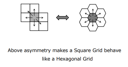
flowchart TD
A["Neighborhood Choice on Square Grid"] --> B{"4-Connectedness vs 8-Connectedness"}
B -->|4-Connectedness| C["Ring Fragmented (4 Objects, 2 Backgrounds) -> Violates Jordan"]
B -->|8-Connectedness| D["Background Leaks Through Diagonals -> Violates Jordan"]
B -->|Asymmetric 6-Connectedness| E["Hexagonal Grid Behavior -> Strict Jordan Conformance"]
style A fill:#1a1a2e,stroke:#e94560,color:#fff
style B fill:#16213e,stroke:#4cc9f0,color:#fff
style C fill:#e94560,stroke:#fff,color:#fff
style D fill:#e94560,stroke:#fff,color:#fff
style E fill:#06d6a0,stroke:#fff,color:#000
2. Sequential Labeling Algorithm
2.1 Algorithm Logic and Neighborhood Rules
Far more efficient and memory-conscious than region growing, Sequential Labeling is a two-pass algorithm. It scans the image in a single pass in raster order.
To label any current pixel $A$, only its previously scanned neighbors—top ($D$), top-left ($C$), and left ($B$)—are inspected:
C D
B A <-- target pixel (A)
Decision rules proceed as follows:
- Background: If $A = 0$, skip without labeling.
- New Object: If $A = 1$ and all neighbors ($B, C, D$) are $0$, assign $A$ a new unique label.
- Top Neighbor Connection: If $A = 1$ and $D$ is labeled, assign $A$ the label of $D$ ($\text{label}(A) = \text{label}(D)$).
- Top-Left Neighbor Connection: If $A = 1$, $D = 0$, and $C$ is labeled, assign $A$ the label of $C$ ($\text{label}(A) = \text{label}(C)$).
- Left Neighbor Connection: If $A = 1$, $D = 0$, $C = 0$, and $B$ is labeled, assign $A$ the label of $B$ ($\text{label}(A) = \text{label}(B)$).
2.2 Conflict Resolution and Equivalence Table
If $A = 1$, $D = 0$, but both $B$ and $C$ are labeled with different tags (e.g., $B = 1$, $C = 2$), a conflict arises. This situation indicates two separate object branches merging at pixel $A$.
Resolution: Assign pixel $A$ one of the two labels (e.g., $B$’s tag). Record the equivalence of tags $1$ and $2$ in an Equivalence Table.
After completing the first pass, the equivalence table is collapsed. A second pass updates all pixel labels to their canonical tags, fully resolving conflicts.
3. Iterative Modification
Local pixel values in a segmented binary image can be modified based on neighbor configurations without breaking topological structure to extract morphological information.
3.1 Euler Number ($E$) and Topological Integrity
The fundamental criterion for maintaining topological integrity is the Euler Number. The Euler number ($E$) is defined as the number of connected object components ($C$) minus the number of holes ($H$):
$$E = \text{Number of Bodies } (C) - \text{Number of Holes } (H)$$
Topological Examples:
- Letter “B”: 1 body, 2 holes $\implies E = 1 - 2 = -1$
- Letter “i”: 2 bodies, 0 holes $\implies E = 2 - 0 = 2$
- Letter “n”: 1 body, 0 holes $\implies E = 1 - 0 = 1$
A crucial property of the Euler number is additivity. Partitioning an image into non-overlapping subregions and summing their individual Euler numbers yields the Euler number of the entire image.
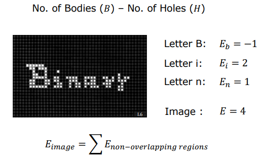
Conservative Operators: Operations that preserve local Euler numbers during pixel modification prevent objects from fusing together or breaking apart.
3.2 Euler Differential ($E^*$) and Neighborhood Classes
The change in the total Euler number caused by changing a pixel from $0$ to $1$ (or $1$ to $0$) is called the Euler Differential ($E^*$).
On a hexagonal pixel grid, each pixel has 6 neighbors, giving $2^6 = 64$ possible neighborhood patterns. These 64 patterns are categorized into 4 classes based on $E^*$:
- $N_{+1}$ Class ($E^ = 1$):* Changing the center pixel from $0$ to $1$ increases $E$ by 1 (creates a new body).
- $N_{0}$ Class ($E^ = 0$):* Changing the center pixel leaves $E$ unchanged. Conservative operations (erasing $1 \to 0$ or adding $0 \to 1$ safely) belong to this class.
- $N_{-1}$ Class ($E^ = -1$):* Setting the center pixel to $1$ connects two separate bodies, decreasing $E$ by 1 ($E^* = -1$).
- $N_{-2}$ Class ($E^ = -2$):* Pixel modification decreases $E$ by 2.
3.3 Parallelization and Three Fields Strategy
Because iterative modification operators are local, pixels can theoretically be updated in parallel. However, updating adjacent pixels simultaneously might produce topological errors (e.g., erasing a two-pixel-thick line entirely).
To prevent this, the pixel grid is partitioned into three fields. Pixels in the first field are updated in parallel, followed by the second and third fields sequentially. This pass repeats until no pixel values change.
3.4 Mathematical Notation, 16 Algorithms, and Thinning (Skeletonization)
To specify an iterative modification algorithm, we select a target neighborhood set $S$ (for conservative operations, $S \in N_0$).
- Let $a_{ij} = 1$ if the neighborhood of pixel $(i,j)$ belongs to $S$, else $a_{ij} = 0$.
- Let $b_{ij}$ be the current pixel value, and $c_{ij}$ the output value.
Combining $(a_{ij}, b_{ij})$ yields 4 possible input pairs, resulting in $2^4 = 16$ distinct output combinations. This defines 16 fundamental iterative modification algorithms.
Two algorithms are of paramount importance:
- Algorithm 7 (Growing / Dilation): With $S \in N_0$, expands object boundaries safely without merging distinct objects.
- Algorithm 4 (Thinning / Skeletonization): With $S \in N_0$, erodes object boundaries inward without creating holes or breaking connectivity. Repeated application reduces objects to a single-pixel topological skeleton.
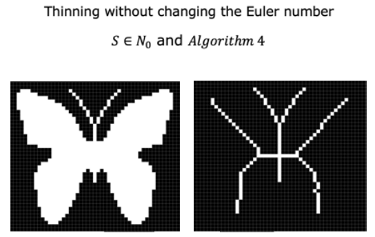
Applications: Skeleton extraction (thinning) is widely applied in human pose estimation, optical character recognition (OCR), and vascular network analysis to compress data volume while retaining shape topology.
Pixel Processing, LSIS, and Continuous Convolution
- 1. Overview of Image Processing
- 2. Pixel / Point Processing
- 3. Linear Shift-Invariant Systems (LSIS)
- 4. Continuous Convolution
- 5. Impulse Response and the Dirac Delta Function
- 6. Fundamental Algebraic Properties of Convolution
- 7. Higher-Dimensional Convolution
1. Overview of Image Processing
Image processing is the transformation of an input image into a new image that is clearer, sharper, or more suitable for visual analysis. In computer vision systems, raw visual data captured by sensors is rarely directly usable; therefore, image processing tools sit “under the hood” of every vision pipeline.
flowchart LR
A["Raw Image <br/> f(x,y)"] --> B["Image Processing <br/> Pipeline"]
B --> C["Enhanced Image <br/> g(x,y)"]
B --> D["Feature Map <br/> Interest Points"]
style A fill:#1a1a2e,stroke:#e94560,color:#fff
style B fill:#16213e,stroke:#0f3460,color:#fff
style C fill:#0f3460,stroke:#e94560,color:#fff
style D fill:#0f3460,stroke:#e94560,color:#fff
The fundamental motivations for image processing fall into two primary categories:
1.1 Image Enhancement
Correcting degradation caused by physical limitations, sensor artifacts, or environment conditions:
- Noise Removal: Cleaning up grainy image data captured under low light conditions.
- Motion Blur Removal: Correcting the smearing effect caused by rapid object motion during the sensor exposure period.
- Defocus Blur Removal: Sharpening blurred images resulting from objects outside the optical camera’s depth of field.
1.2 Information Recovery
Exposing and highlighting the most critical, distinctive attributes (salient features) for downstream analysis or object detection. This includes detecting and enhancing edges, corners, and keypoints.
Key Insight: Image processing alters spatial pixel structures to optimize images for both human perception and downstream algorithmic evaluation.
2. Pixel / Point Processing
Pixel (or point) processing is the simplest and computationally cheapest class of operations applied to an image. Its core principle is to transform each pixel independently based solely on its own intensity or color value, completely ignoring its spatial coordinates and neighbor values.
flowchart TD
In["Pixel f(x,y)"] --> T["Transfer Function T(f)"] --> Out["Pixel g(x,y)"]
style In fill:#1a1a2e,stroke:#e94560,color:#fff
style T fill:#16213e,stroke:#0f3460,color:#fff
style Out fill:#0f3460,stroke:#e94560,color:#fff
In continuous space, an image is defined as an intensity function $f(x,y)$. The point processing transformation is expressed as:
$$g(x,y) = T(f(x,y))$$
where $f(x,y)$ is the input image, $g(x,y)$ is the output image, and $T$ represents the point-wise transfer function. For RGB color images, this transformation can be applied independently across Red ($R$), Green ($G$), and Blue ($B$) channels.
2.1 Common Pixel Processing Transformations
Darken
Subtracting a fixed intensity constant $C$ from every pixel value:
$$g(x,y) = f(x,y) - C \quad (\text{e.g., } f(x,y) - 128)$$
Lighten
Adding a fixed intensity constant $C$ to every pixel value:
$$g(x,y) = f(x,y) + C \quad (\text{e.g., } f(x,y) + 128)$$
Image Invert / Negative
Reversing intensity values in an 8-bit image system:
$$g(x,y) = 255 - f(x,y)$$
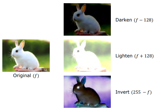
Lower Contrast
Compressing the dynamic range of intensity values (e.g., dividing all pixel values by 2):
$$g(x,y) = \frac{f(x,y)}{2}$$
High Contrast
Expanding the dynamic range of intensity values by multiplying pixel intensities by a scale factor:
$$g(x,y) = f(x,y) \times 2$$
Warning: Saturation & Clipping Issue
When increasing contrast, pixel values may exceed the maximum allowable dynamic range (255 for 8-bit systems). Any value greater than 255 is clipped directly to 255, resulting in detail loss and overexposed white regions (saturation):$$g(x,y) = \min(255, \max(0, T(f(x,y))))$$
Grayscale Conversion
Combining RGB color channels using weights derived from human photopic vision sensitivity curves:
$$g(x,y) = 0.3 \cdot R(x,y) + 0.6 \cdot G(x,y) + 0.1 \cdot B(x,y)$$
3. Linear Shift-Invariant Systems (LSIS)
Linear Shift-Invariant Systems (LSIS) constitute the foundational system architecture for the vast majority of signal and computer vision algorithms. The transformation of an input $f(x)$ into an output $g(x)$ via an LSIS relies on two fundamental mathematical axioms.
3.1 Linearity
The system must satisfy superposition and scaling principles. Assume system response $\text{LSIS}(f_1(x)) = g_1(x)$ and $\text{LSIS}(f_2(x)) = g_2(x)$:
For any linear combination $\alpha f_1(x) + \beta f_2(x)$, the output must equal the exact same linear combination of individual outputs:
$$\text{LSIS}(\alpha f_1(x) + \beta f_2(x)) = \alpha \cdot g_1(x) + \beta \cdot g_2(x)$$
3.2 Shift Invariance
A spatial shift in the input signal must produce an identical spatial shift in the output response:
$$\text{LSIS}(f(x - a)) = g(x - a)$$
3.3 Physical Example: Ideal Lens System
An ideal lens system provides a clear physical example of an LSIS:
- Linearity: Increasing scene illumination linearly scales focused image brightness ($f$) and defocused image brightness ($g$) by the exact same proportion.
- Shift Invariance: Shifting an object in the scene laterally or vertically shifts its projected image by the exact same spatial offset in both focused and blurred states.
4. Continuous Convolution
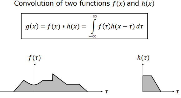
Mathematically, any LSIS performs convolution, and any system performing convolution is an LSIS. The continuous 1D convolution of two functions $f(x)$ and $h(x)$ is defined as:
$$g(x) = f(x) * h(x) = \int_{-\infty}^{\infty} f(\tau) , h(x - \tau) , d\tau$$
4.1 Geometric Steps of Convolution
Computing continuous convolution geometrically involves 5 steps:
flowchart TD
S1["1. Variable Transformation: f(τ) & h(τ)"] --> S2["2. Flip: h(-τ)"]
S2 --> S3["3. Shift: h(x - τ)"]
S3 --> S4["4. Multiply & Integrate: ∫ f(τ) h(x-τ) dτ"]
S4 --> S5["5. Slide x across domain"]
style S1 fill:#1a1a2e,stroke:#e94560,color:#fff
style S2 fill:#16213e,stroke:#0f3460,color:#fff
style S3 fill:#16213e,stroke:#0f3460,color:#fff
style S4 fill:#0f3460,stroke:#e94560,color:#fff
style S5 fill:#0f3460,stroke:#e94560,color:#fff
- Variable Transformation: Express functions in terms of integration variable $\tau$ ($f(\tau)$ and $h(\tau)$).
- Flip: Katlanmış function $h(-\tau)$ is obtained by flipping $h(\tau)$ symmetrically about the vertical axis.
- Shift: Shift the flipped function by $x$ to form $h(x - \tau)$.
- Multiply & Integrate: Overlay $h(x-\tau)$ on $f(\tau)$, compute the point-wise product, and integrate to evaluate the output intensity $g(x)$.
- Slide: Sweep $x$ continuously from $-\infty$ to $+\infty$ to map out the entire function $g(x)$.
4.2 Convolution Examples
Convolution of Two Identical Box Functions
Consider two identical centered rectangular pulses of width 2 and height 1:
$$f(x) = \begin{cases} 1, & |x| \leq 1 \ 0, & |x| > 1 \end{cases} \quad \text{and} \quad h(x) = \begin{cases} 1, & |x| \leq 1 \ 0, & |x| > 1 \end{cases}$$
- As $h(x-\tau)$ slides from $-\infty$, overlap begins at $x = -2$.
- Overlap area increases linearly as $x$ moves toward 0.
- At $x = 0$, maximum overlap occurs with peak area equal to $\text{width} \times \text{height} = 2 \times 1 = 2$.
- Overlap decreases linearly until reaching zero at $x = 2$.
- Result: A symmetric triangular pulse centered at $x=0$ with height 2 and base width 4.
Convolution of a Box and a Triangle
When convolving a centered rectangle with a triangle:
- As the triangle slides into the rectangular region, both base width and overlap height grow linearly with offset $x$.
- Result: The resulting overlap integral is quadratic in $x$.
4.3 Proof: Convolution is an LSIS
1. Proof of Linearity
Let input signal $f_{\text{in}}(\tau) = \alpha f_1(\tau) + \beta f_2(\tau)$. Output:
$$g(x) = \int_{-\infty}^{\infty} [\alpha f_1(\tau) + \beta f_2(\tau)] , h(x-\tau) , d\tau$$
Applying integral linearity:
$$g(x) = \alpha \int_{-\infty}^{\infty} f_1(\tau) , h(x-\tau) , d\tau + \beta \int_{-\infty}^{\infty} f_2(\tau) , h(x-\tau) , d\tau$$
$$g(x) = \alpha \cdot g_1(x) + \beta \cdot g_2(x)$$
Superposition holds; convolution is linear.
2. Proof of Shift Invariance
Shift the input signal by $a$: $f_{\text{new}}(\tau) = f(\tau - a)$. Output:
$$g_{\text{new}}(x) = \int_{-\infty}^{\infty} f(\tau - a) , h(x - \tau) , d\tau$$
Substitute $\mu = \tau - a$ ($d\mu = d\tau$ and $\tau = \mu + a$):
$$g_{\text{new}}(x) = \int_{-\infty}^{\infty} f(\mu) , h(x - (\mu + a)) , d\mu = g(x - a)$$
Input shift by $a$ produces an identical output shift by $a$. System is shift-invariant.
5. Impulse Response and the Dirac Delta Function
To completely characterize an unknown LSIS (“black box”), a special probe signal is passed through the system: the Unit Impulse Function ($\text{Dirac Delta} - \delta(x)$).
flowchart LR
Delta["Dirac Delta δ(x)"] --> System["Black Box LSIS"] --> Impulse["Impulse Response h(x)"]
style Delta fill:#1a1a2e,stroke:#e94560,color:#fff
style System fill:#16213e,stroke:#0f3460,color:#fff
style Impulse fill:#0f3460,stroke:#e94560,color:#fff
5.1 Dirac Delta Function Properties
Mathematically, the Dirac delta function represents the limiting case of a rectangular pulse of infinitely narrow width ($2\varepsilon$) and infinitely high amplitude ($1/(2\varepsilon)$) as $\varepsilon \to 0$, such that total area is unity:
$$\int_{-\infty}^{\infty} \delta(x) , dx = 1$$
The fundamental property of the delta function is the Sifting Property:
$$\int_{-\infty}^{\infty} b(\tau) , \delta(x - \tau) , d\tau = b(x)$$
The impulse isolates and sifts out the exact function value $b(x)$ at the impulse point.
5.2 System Characterization via Impulse Response ($h$)
When unit impulse $\delta(x)$ is applied to an unknown LSIS, the sifting property yields the system’s own transfer function:
$$g(x) = \delta(x) * h(x) = h(x)$$
The function $h(x)$ is called the Impulse Response. Once $h(x)$ is measured, system behavior for any arbitrary input $f(x)$ is fully determined as $f(x) * h(x)$.
5.3 Optical & Biological Application: Human Eye PSF
Because optical lenses form a 2D LSIS, the human eye behaves as a 2D LSIS.
- Star Example: Observing a distant star provides a physical 2D point impulse excitation ($\delta(x,y)$).
- The 2D image projected onto the retina by a point source is the Point Spread Function (PSF).
- A healthy eye has an extremely narrow PSF (decaying within $0.05^\circ$), ensuring sharp vision. Broader PSFs cause blurred perception.
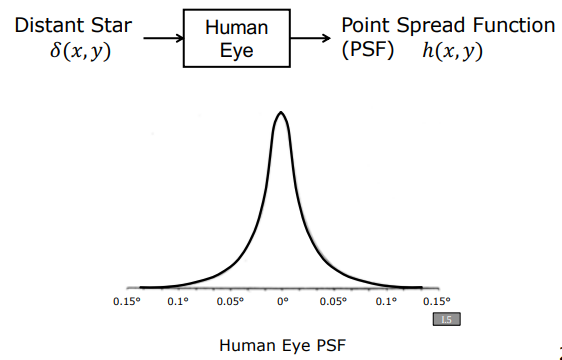
6. Fundamental Algebraic Properties of Convolution
6.1 Commutative
$$f * h = h * f$$
6.2 Associative
$$(f * h_1) * h_2 = f * (h_1 * h_2)$$
6.3 Cascaded Systems
For a sequence of filters $h_1$ and $h_2$, cascading permits combining filters into a single equivalent impulse response $h_{\text{eq}} = h_1 * h_2$, reducing computation:
flowchart LR
subgraph A1 ["Sequential Operations"]
f1["f(x)"] --> H1["h1(x)"] --> H2["h2(x)"] --> g1["g(x)"]
end
subgraph A2 ["Single Equivalent Filter"]
f2["f(x)"] --> Heq["heq = h1 * h2"] --> g2["g(x)"]
end
style H1 fill:#16213e,stroke:#0f3460,color:#fff
style H2 fill:#16213e,stroke:#0f3460,color:#fff
style Heq fill:#0f3460,stroke:#e94560,color:#fff
7. Higher-Dimensional Convolution
Because images are 2D spatial signals, continuous 2D convolution is defined as:
$$g(x,y) = f(x,y) * h(x,y) = \int_{-\infty}^{\infty} \int_{-\infty}^{\infty} f(\tau, \mu) , h(x - \tau, y - \mu) , d\tau , d\mu$$
Key Insight: This formulation extends naturally to 3D volumetric images (e.g., MRI, CT, Ultrasound) by evaluating integrals across 3 spatial dimensions.
Linear and Non-Linear Image Filters
- 1. Discrete 2D Convolution
- 2. Border Problems
- 3. Classic Linear Filter Types
- 4. Gaussian Smoothing
- 5. Non-Linear Filters
1. Discrete 2D Convolution
In computer vision applications, images are processed as discrete 2D pixel matrices rather than continuous mathematical functions. For an $M \times N$ image $f[i,j]$ and a filter kernel $h[i,j]$, discrete 2D convolution is defined as:
$$g[i,j] = f[i,j] * h[i,j] = \sum_{m} \sum_{n} f[m,n] , h[i - m, j - n]$$
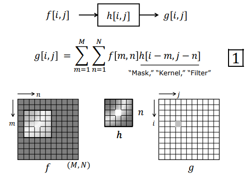
where $i$ represents row indices and $j$ represents column indices.
flowchart TD
Step1["1. Double Flip: h[-m, -n]"] --> Step2["2. Overlay: Center over pixel f[i,j]"]
Step2 --> Step3["3. Pointwise Multiplication"]
Step3 --> Step4["4. Sum -> g[i,j]"]
Step4 --> Step5["5. Raster Scan Across Image"]
style Step1 fill:#1a1a2e,stroke:#e94560,color:#fff
style Step2 fill:#16213e,stroke:#0f3460,color:#fff
style Step3 fill:#16213e,stroke:#0f3460,color:#fff
style Step4 fill:#0f3460,stroke:#e94560,color:#fff
style Step5 fill:#0f3460,stroke:#e94560,color:#fff
1.1 Discrete Convolution Pipeline
Executing discrete 2D convolution follows 5 programmatic steps:
- Double Flip: Flip the filter kernel $h$ horizontally ($m$) and vertically ($n$) to form $h[-m, -n]$.
- Overlay: Center the flipped kernel over target pixel $[i,j]$.
- Multiply: Multiply kernel weights element-wise with overlapping pixel intensity values.
- Sum: Sum all multiplication results and assign the value to output pixel $g[i,j]$.
- Raster Scan: Slide the kernel across the entire image grid from left-to-right and top-to-bottom.
2. Border Problems
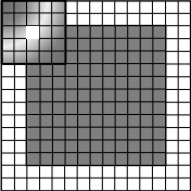
When a filter kernel centers over boundary pixels, portions of the kernel extend beyond the spatial dimensions of the image where no pixel intensity data exists.
flowchart LR
A["Image Boundary"] --- B["Ignore Border <br/> Cropped Output"]
A --- C["Constant Padding <br/> Zero Padding"]
A --- D["Reflection Padding <br/> Mirroring"]
style A fill:#1a1a2e,stroke:#e94560,color:#fff
style B fill:#16213e,stroke:#0f3460,color:#fff
style C fill:#16213e,stroke:#0f3460,color:#fff
style D fill:#0f3460,stroke:#e94560,color:#fff
Three standard approaches are used to resolve boundary conditions:
2.1 Ignore Border
Compute convolution only for interior pixels where the entire kernel fits strictly inside the image frame. The resulting output image is cropped along its perimeter by the kernel radius.
2.2 Constant / Zero Padding
Pad the regions outside the image boundaries with a constant value (commonly 0 for black or the mean image intensity).
2.3 Reflection Padding
Mirror boundary pixels across the edge boundary. Reflection padding produces the most natural transition and prevents artificial boundary seam artifacts.
3. Classic Linear Filter Types
3.1 Impulse Filter
A kernel containing 1 at its center cell and 0 elsewhere passes the input image through unchanged due to the sifting property:
$$g[i,j] = f[i,j] * \delta[i,j] = f[i,j]$$
3.2 Shift Filter
Placing the unit impulse at the bottom-right corner of the kernel shifts the output image down and to the right by 1 pixel, due to the double-flip nature of convolution:
$$h = \begin{bmatrix} 0 & 0 & 0 \ 0 & 0 & 0 \ 0 & 0 & 1 \end{bmatrix} \implies g[i,j] = f[i-1, j-1]$$
3.3 Box / Averaging Filter
Used to smooth spatial noise across local pixel neighborhoods. Consider an unnormalized $5 \times 5$ box kernel with all entries set to 1:
$$h_{\text{unnorm}} = \begin{bmatrix} 1 & 1 & 1 & 1 & 1 \ \vdots & & \ddots & & \vdots \ 1 & 1 & 1 & 1 & 1 \end{bmatrix}$$
Warning: Saturation and Normalization
Applying an unnormalized box filter causes output pixel values to scale up by $25\times$, exceeding the 8-bit dynamic range (255) and resulting in total white saturation.
Solution: The sum of all kernel weights must equal 1. Divide each element by the total kernel area ($25$):
$$h_{\text{box}} = \frac{1}{25} \begin{bmatrix} 1 & 1 & 1 & 1 & 1 \ \vdots & & \ddots & & \vdots \ 1 & 1 & 1 & 1 & 1 \end{bmatrix}$$
Key Insight: Large box filters (e.g., $21 \times 21$) introduce rectangular boxy artifacts due to sharp square boundaries in spatial domain filtering.
4. Gaussian Smoothing
To eliminate rectangular boxy artifacts, Gaussian smoothing uses a rotationally symmetric, smooth kernel whose weights decay gracefully from the center pixel.
4.1 Gaussian Kernel Mathematics
In 2D discrete space, a Gaussian filter kernel is defined as:
$$G_{\sigma}[i,j] = \frac{1}{2\pi\sigma^2} e^{-\frac{i^2 + j^2}{2\sigma^2}}$$
where:
- $i, j$: Row and column spatial distance offsets from the kernel center.
- $\sigma$ (Standard Deviation): Controls kernel spread (smoothing width); $\sigma^2$ represents variance.
- $\frac{1}{2\pi\sigma^2}$: Normalization factor ensuring total volume under the 2D Gaussian sums to 1.
4.2 Kernel Window Size Selection ($K \times K$)
Although continuous Gaussians extend to infinity, finite discrete kernels capture $99.7%$ of Gaussian energy using the standard rule of thumb:
$$K \approx 2\pi\sigma \quad (\text{or } K \approx 6\sigma)$$
4.3 Gaussian Filter Separability
A key property of Gaussian filters in computer vision is separability.
Mathematical Proof
The 2D Gaussian exponent decomposes into the product of two 1D Gaussian exponents:
$$e^{-\frac{m^2 + n^2}{2\sigma^2}} = e^{-\frac{m^2}{2\sigma^2}} \cdot e^{-\frac{n^2}{2\sigma^2}}$$
Substituting into the discrete 2D convolution equation:
$$g[i,j] = \sum_{m} \sum_{n} f[m,n] \cdot \left( \frac{1}{2\pi\sigma^2} e^{-\frac{(i-m)^2 + (j-n)^2}{2\sigma^2}} \right)$$
$$g[i,j] = \frac{1}{2\pi\sigma^2} \sum_{m} e^{-\frac{(i-m)^2}{2\sigma^2}} \left( \sum_{n} f[m,n] \cdot e^{-\frac{(j-n)^2}{2\sigma^2}} \right)$$
Convolving an image with a $K \times K$ 2D Gaussian kernel is mathematically identical to applying a 1D horizontal Gaussian filter of length $K$, followed by a 1D vertical Gaussian filter of length $K$:
$$\text{2D } G_{\sigma} \equiv \text{1D Horizontal } G_{\sigma} * \text{1D Vertical } G_{\sigma}$$
flowchart LR
A["Image f[i,j]"] --> B["1D Horizontal Gaussian <br/> (K multiplications)"]
B --> C["1D Vertical Gaussian <br/> (K multiplications)"]
C --> D["Output g[i,j]"]
style A fill:#1a1a2e,stroke:#e94560,color:#fff
style B fill:#16213e,stroke:#0f3460,color:#fff
style C fill:#16213e,stroke:#0f3460,color:#fff
style D fill:#0f3460,stroke:#e94560,color:#fff
Computational Complexity Comparison (Per Pixel)
For a $K \times K$ filter window:
- Non-Separable Direct 2D Filter:
- Multiplications: $K^2$
- Additions: $K^2 - 1$
- Separable 1D + 1D Filter:
- Multiplications: $2K$
- Additions: $2(K - 1)$
Performance Optimization Example ($K = 21$):
- Direct 2D: $21^2 = 441$ multiplications, $440$ additions.
- Separable 1D + 1D: $2 \times 21 = 42$ multiplications, $40$ additions.
Speedup: Approximately $10.5\times$ fewer operations per pixel!
5. Non-Linear Filters
Linear convolution filters suppress noise by attenuating high spatial frequencies, which inadvertently blurs sharp object edges. Non-linear algorithmic filters overcome this trade-off.
5.1 Median Filter
Random black (0) or white (255) corrupted pixels are referred to as Salt and Pepper Noise.
flowchart TD
Sub1["1. Extract K x K Neighborhood"] --> Sub2["2. Sort Pixel Values Ascending"]
Sub2 --> Sub3["3. Select Median (Middle) Value"]
Sub3 --> Sub4["4. Assign Median to Target Pixel"]
style Sub1 fill:#1a1a2e,stroke:#e94560,color:#fff
style Sub2 fill:#16213e,stroke:#0f3460,color:#fff
style Sub3 fill:#0f3460,stroke:#e94560,color:#fff
style Sub4 fill:#0f3460,stroke:#e94560,color:#fff
- Linear Filter Limitation: Gaussian or box filters smear outlier impulse values across neighborhoods, muddying the image without removing noise spikes.
- Median Filter Mechanism: Sort all pixel intensities within a $K \times K$ local window in ascending order and assign the median value to the output pixel.
- Why It Works: Outlier salt (255) and pepper (0) values sit at the extreme ends of sorted lists, making their selection as median values statistically impossible. Noise is removed cleanly without degrading edges.
- Drawback: Excessively large median window sizes (e.g., $11 \times 11$) produce watercolor/painterly artifacts that destroy fine detail.
5.2 Bilateral Filter
The Bilateral Filter is an edge-preserving non-linear filter that smooths noise in uniform spatial regions while preserving sharp high-frequency edges.
flowchart LR
Gs["Spatial Gaussian Gs <br/> (Physical Distance)"] --> Mult["Product <br/> Gs x Gr"]
Gr["Range Gaussian Gr <br/> (Intensity Difference)"] --> Mult
Mult --> Out["Edge-Preserving Kernel"]
style Gs fill:#1a1a2e,stroke:#e94560,color:#fff
style Gr fill:#16213e,stroke:#0f3460,color:#fff
style Mult fill:#0f3460,stroke:#e94560,color:#fff
style Out fill:#0f3460,stroke:#e94560,color:#fff
Dual Gaussian Mechanism
Standard Gaussian smoothing relies solely on spatial proximity ($G_s$), whereas Bilateral filtering weights pixels by both spatial proximity ($G_s$) and intensity similarity ($G_r$):
$$g[i,j] = \frac{1}{W[i,j]} \sum_{m} \sum_{n} f[i-m, j-n] \cdot G_s[m,n] \cdot G_r[m,n]$$
where:
-
Spatial Gaussian ($G_s$): Weights pixels based on geometric distance:
$$G_s[m,n] = e^{-\frac{m^2 + n^2}{2\sigma_s^2}}$$
-
Range / Brightness Gaussian ($G_r$): Weights pixels based on photometric intensity differences relative to the central pixel:
$$G_r[m,n] = e^{-\frac{(f[i-m, j-n] - f[i,j])^2}{2\sigma_r^2}}$$
Dynamic Normalization Factor ($W[i,j]$)
Because kernel weights truncate near sharp boundaries ($G_r \to 0$ across step edges), the normalization constant is recalculated at every pixel position to maintain unit kernel energy:
$$W[i,j] = \sum_{m} \sum_{n} G_s[m,n] \cdot G_r[m,n]$$
Edge-Preserving Intuition
When the kernel centers near a step edge:
- Pixels on the same side of the boundary share similar intensity values $\implies G_r \approx 1$.
- Pixels on the opposite side of the boundary differ significantly in intensity $\implies G_r \approx 0$.
- Result: The kernel truncates along boundary edges, preventing blurring across edge transitions.
Parameter Limiting Behavior
- Increasing $\sigma_s$ increases smoothing across uniform regions.
- As $\sigma_r \to \infty$, $G_r[m,n] \to 1$, reducing the Bilateral filter directly to a standard linear Gaussian filter.
5.3 Comparison: Gaussian vs. Bilateral Filtering
Template Matching
- 1. The Template Matching Problem
- 2. Sum of Squared Differences (SSD)
- 3. Cross-Correlation
- 4. Limitation of Unnormalized Cross-Correlation
- 5. Normalized Cross-Correlation (NCC)
1. The Template Matching Problem
Template matching is the task of identifying the exact spatial location of a small template image $T[u,v]$ (a pattern or patch) within a larger target image $f[x,y]$.
flowchart LR
Target["Target Image f[x,y]"] --> Slide["Slide Template T[u,v] Across Grid"]
Slide --> Metric["Compute Similarity Metric"]
Metric --> Peak["Optimal Match Coordinates (i*, j*)"]
style Target fill:#1a1a2e,stroke:#e94560,color:#fff
style Slide fill:#16213e,stroke:#0f3460,color:#fff
style Metric fill:#16213e,stroke:#0f3460,color:#fff
style Peak fill:#0f3460,stroke:#e94560,color:#fff
Physical Scenario
Locating the King face region ($T[u,v]$ template) within an image of a full playing card deck ($f[x,y]$) and returning its bounding coordinates is a standard template matching application.
2. Sum of Squared Differences (SSD)
The most direct way to measure geometric and color mismatch between a template and an overlapping image patch is by computing the Sum of Squared Differences (SSD).
For a spatial offset $(i,j)$, the error metric $E[i,j]$ is defined as:
$$E[i,j] = \sum_{m} \sum_{n} \left( f[m,n] - T[m-i, n-j] \right)^2$$
Key Insight: As the error metric $E[i,j]$ approaches zero ($E[i,j] \to 0$), the local image region aligns perfectly with the template pattern.
2.1 Algebraic Expansion of SSD
Expanding the squared term and distributing summations yields:
$$E[i,j] = \sum_{m}\sum_{n} \left( f^2[m,n] + T^2[m-i, n-j] - 2 \cdot f[m,n] \cdot T[m-i, n-j] \right)$$
$$E[i,j] = \sum_{m}\sum_{n} f^2[m,n] + \sum_{m}\sum_{n} T^2[m-i, n-j] - 2 \sum_{m}\sum_{n} f[m,n] \cdot T[m-i, n-j]$$
Analyzing the expanded terms:
- $\sum \sum T^2$ (Template Energy): Total energy of the template $T$, which remains constant across all spatial shifts.
- $\sum \sum f^2$ (Local Image Energy): Total energy of the local image patch beneath the template window.
- $-2 \sum \sum f \cdot T$ (Cross Term): Possesses a negative ($-$) sign in the expanded expression.
Minimizing the error metric $E[i,j]$ is algebraically equivalent to maximizing the third term ($\sum \sum f \cdot T$). This third term represents the Cross-Correlation between the template and the image.
3. Cross-Correlation
Cross-Correlation ($\otimes$) computes the direct dot product between overlapping image and template pixels:
$$R[i,j] = f[i,j] \otimes T[i,j] = \sum_{m} \sum_{n} f[m,n] \cdot T[m-i, n-j]$$
flowchart TD
subgraph Conv ["Convolution (*)"]
C1["Flip Kernel Horizontally & Vertically (Double Flip)"] --> C2["Overlay & Compute Dot Products"]
end
subgraph Corr ["Correlation (⊗)"]
K1["Take Template As-Is (No Flip)"] --> K2["Overlay & Compute Dot Products Directly"]
end
style C1 fill:#1a1a2e,stroke:#e94560,color:#fff
style C2 fill:#16213e,stroke:#0f3460,color:#fff
style K1 fill:#16213e,stroke:#0f3460,color:#fff
style K2 fill:#0f3460,stroke:#e94560,color:#fff
3.1 Convolution vs. Correlation
While similar mathematically, the two operations differ fundamentally:
-
Convolution ($*$): The kernel is flipped horizontally and vertically before overlaying onto the image:
$$g[i,j] = f[i,j] * h[i,j] = \sum_{m} \sum_{n} f[m,n] \cdot h[i-m, j-n]$$
-
Correlation ($\otimes$): The template is applied directly without flipping (no flipping):
$$R[i,j] = f[i,j] \otimes T[i,j] = \sum_{m} \sum_{n} f[m,n] \cdot T[m-i, n-j]$$
4. Limitation of Unnormalized Cross-Correlation
Direct unnormalized cross-correlation ($R[i,j]$) fails as a standalone matching metric because it is overly sensitive to absolute pixel intensity values.
flowchart TD
T["Template T: Low-High-Low Pattern"]
A["Region A: Perfect Match, Low Brightness"]
B["Region B: Partial Match, Medium Brightness"]
C["Region C: No Match, Extremely Bright White"]
T --> A & B & C
A -->|Direct Correlation| RA["R(A) Low Score"]
B -->|Direct Correlation| RB["R(B) Medium Score"]
C -->|Direct Correlation| RC["R(C) Highest Score! (FAILURE)"]
style T fill:#1a1a2e,stroke:#e94560,color:#fff
style A fill:#16213e,stroke:#0f3460,color:#fff
style B fill:#16213e,stroke:#0f3460,color:#fff
style C fill:#0f3460,stroke:#e94560,color:#fff
style RC fill:#e94560,stroke:#fff,color:#fff
4.1 Counter-Example
Consider a 1D template $T$ evaluated against three candidate image regions ($A$, $B$, $C$):
- $T$ (Template): Low-High-Low amplitude pattern.
- Region $A$: Structurally identical pattern, but low overall intensity (dim).
- Region $B$: Partial pattern match, moderate intensity.
- Region $C$: Irrelevant pattern, but extremely high pixel intensity (bright white).
Direct Correlation Ranking:
Because raw multiplication scales with absolute pixel values, unnormalized correlation yields:
$$R_C > R_B > R_A$$
The system falsely flags Region $C$ as the best match, despite having zero structural relation to the template.
5. Normalized Cross-Correlation (NCC)
To eliminate intensity bias, the correlation score is normalized by dividing by the square root of the product of local image energy and template energy:
$$R_{\text{NCC}}[i,j] = \frac{\sum_{m} \sum_{n} f[m,n] \cdot T[m-i, n-j]}{\sqrt{\left( \sum_{m} \sum_{n} f^2[m,n] \right) \cdot \left( \sum_{m} \sum_{n} T^2[m-i, n-j] \right)}}$$
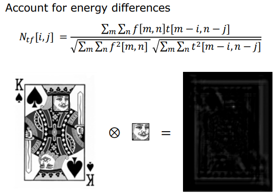
5.1 Properties & Robustness of NCC
The denominator normalization provides key advantages:
-
Illumination Invariance: Robust against changes in ambient lighting or shadows.
-
Gain Independence: Invariant to linear camera gain and contrast adjustments.
-
Correct Pattern Ranking: Normalization attenuates raw brightness effects, yielding the true match ranking:
$$R_{\text{NCC}}(A) > R_{\text{NCC}}(B) > R_{\text{NCC}}(C)$$
Key Insight: The peak correlation response ($R_{\text{NCC}} \to 1.0$) in the NCC output map corresponds precisely to the center spatial coordinates of the matched template.
Overview, Fourier Transform, and Convolution Theorem
- 1. Overview of Frequency Domain
- 2. Fourier Transform
- 3. Square Wave Construction & Fourier Series
- 4. Mathematical Formulation and Proofs
- 5. Complex Structure of Fourier Transform
- 6. Fundamental Fourier Transform Pairs
- 7. Fundamental Properties of Fourier Transform
- 8. Convolution Theorem
1. Overview of Frequency Domain
Analyzing images exclusively in the spatial domain (pixel-by-pixel intensity operations) can be computationally expensive and conceptually complex for operations like blurring, sharpening, or deconvolution. The frequency domain provides an alternative representation by expressing spatial image structures as a weighted sum of sinusoids (sine and cosine waves) across various spatial frequencies.
flowchart TD
A["Spatial Domain Image <br/> f(x,y)"] -->|"Fourier Transform <br/> (Forward FT)"| B["Frequency Domain <br/> F(u,v)"]
B -->|"Frequency Filtering <br/> H(u,v)"| C["Filtered Spectrum <br/> G(u,v)"]
C -->|"Inverse Fourier Transform <br/> (Inverse FT)"| D["Enhanced Image <br/> g(x,y)"]
style A fill:#1a1a2e,stroke:#e94560,color:#fff
style B fill:#16213e,stroke:#0f3460,color:#fff
style C fill:#0f3460,stroke:#e94560,color:#fff
style D fill:#16213e,stroke:#4cc9f0,color:#fff
Transitioning from spatial coordinates to frequency representation yields three core engineering advantages:
- Convolution Efficiency: Computationally intensive spatial convolution integrals are converted into simple point-wise multiplication in the frequency domain.
- Frequency Separation: High-frequency components (fine details, sharp edges, granular noise) and low-frequency components (smooth backgrounds, slow intensity gradients) are explicitly isolated in separate spectral regions.
- Restoration & Deconvolution Stability: Image restoration, motion deblurring, and inverse filtering become mathematically tractable and stable.
Key Insight: Spatial domain operations observe where intensity changes occur, while frequency domain operations analyze how fast intensity changes occur across space.
2. Fourier Transform
The Fourier Transform is named after the French mathematician and physicist Jean Baptiste Joseph Fourier (1768–1830).
2.1 Historical Background
Fourier introduced his foundational concept while modeling heat diffusion through solid materials. He claimed that any periodic function could be represented as an infinite sum of sinusoidal waves.
Prominent mathematicians of his era—including Joseph-Louis Lagrange and Leonhard Euler—initially rejected Fourier’s work as lacking mathematical rigor. It took nearly eight years for his papers to achieve publication. Today, the Fourier Transform serves as a fundamental pillar across signal processing, computer vision, communications, and physics.
2.2 Fundamental Principle: Sinusoidal Building Blocks
At the heart of Fourier analysis lies the sinusoid. A continuous 1D sinusoidal signal is mathematically defined as:
$$f(x) = A \sin(2\pi u x + \phi)$$
where:
- $A$ (Amplitude): Represents the peak height or maximum power of the wave.
- $u$ (Frequency): Dictates the number of oscillation cycles per unit spatial distance.
- $T = \frac{1}{u}$ (Period): Represents the spatial distance required for one complete oscillation cycle.
- $\phi$ (Phase): Specifies the angular phase shift relative to the origin.
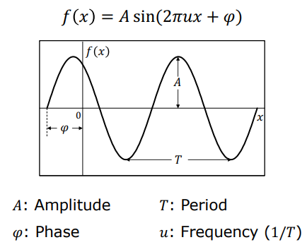
3. Square Wave Construction & Fourier Series
A classic illustration of Fourier theory is constructing a periodic square wave by summing simple sine waves at fundamental and harmonic frequencies.
flowchart LR
A["Fundamental Sinusoid <br/> u"] --> B["Add 3rd Harmonic <br/> 3u"]
B --> C["Add 5th & 7th Harmonics <br/> 5u, 7u"]
C --> D["Infinite Harmonics <br/> N → ∞"]
D --> E["Ideal Square Wave"]
style A fill:#1a1a2e,stroke:#e94560,color:#fff
style B fill:#16213e,stroke:#0f3460,color:#fff
style C fill:#0f3460,stroke:#e94560,color:#fff
style D fill:#16213e,stroke:#4cc9f0,color:#fff
style E fill:#0f3460,stroke:#4cc9f0,color:#fff
- 1 Sinusoid: Adding only the fundamental frequency $u$ yields a coarse, smooth approximation of the square wave.
- Successive Odd Harmonics: Adding odd harmonics ($u, 3u, 5u, 7u, \dots$) with progressively decreasing amplitudes ($\frac{1}{1}, \frac{1}{3}, \frac{1}{5}, \frac{1}{7}, \dots$) flattens the wave crests and steepens vertical transitions.
- 8 Sinusoids: Summing the first 8 harmonic terms produces a profile that closely resembles a sharp square wave.
- Infinite Terms: Summing an infinite series of sinusoids yields an exact square wave with perfectly vertical step discontinuities.
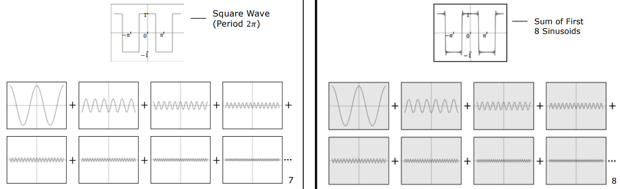
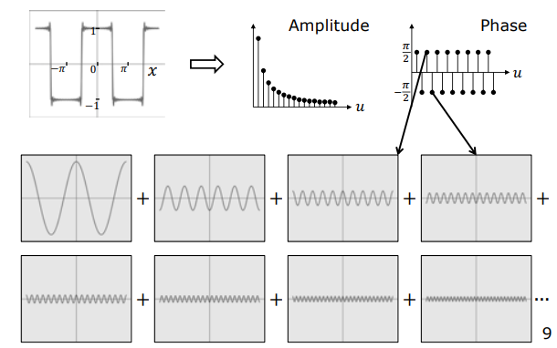
Warning: Ringing Artifacts & Gibbs Phenomenon
Representing an instantaneous spatial step discontinuity (such as the vertical edge of a square wave) requires infinitely high frequencies. Truncating the Fourier series to a finite number of harmonics introduces high-frequency oscillations near sharp boundaries, known as ringing artifacts or the Gibbs Phenomenon. Additionally, the phase $\phi$ of harmonics in a square wave alternates between $-\pi/2$ and $\pi/2$.
4. Mathematical Formulation and Proofs
The Fourier Transform maps a continuous spatial signal $f(x)$ to its frequency domain representation $F(u)$ without any loss of information.
4.1 1D Continuous Fourier Transform (Forward & Inverse)
The Forward Fourier Transform (1D FT) converts a spatial function $f(x)$ into the frequency domain $F(u)$:
$$F(u) = \int_{-\infty}^{\infty} f(x) e^{-i 2\pi u x} , dx$$
The Inverse Fourier Transform (1D IFT) reconstructs the original spatial signal $f(x)$ from its frequency spectrum $F(u)$:
$$f(x) = \int_{-\infty}^{\infty} F(u) e^{i 2\pi u x} , du$$
where $x$ denotes spatial position and $u$ represents spatial frequency.
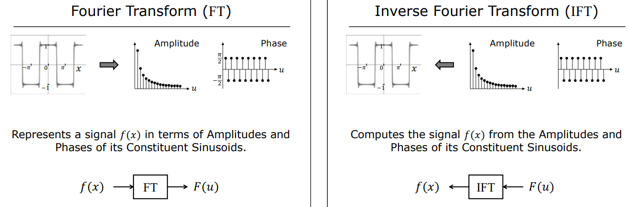
Mathematical Symmetry Note: The forward transform uses $-i$ in the complex exponential exponent, whereas the inverse transform uses $+i$.
4.2 Derivation of Euler’s Formula via Taylor Series
To understand why complex exponentials ($e^{i\theta}$) represent sinusoidal waves ($\cos\theta, \sin\theta$), we use Euler’s Formula:
$$e^{i\theta} = \cos\theta + i\sin\theta \quad (\text{where } i = \sqrt{-1})$$
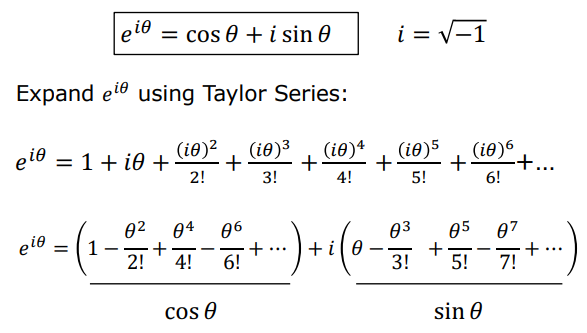
Step-by-Step Proof:
The Maclaurin (Taylor series around $x=0$) expansion for $e^x$ is:
$$e^{x} = 1 + x + \frac{x^2}{2!} + \frac{x^3}{3!} + \frac{x^4}{4!} + \frac{x^5}{5!} + \dots$$
Substituting $x = i\theta$:
$$e^{i\theta} = 1 + (i\theta) + \frac{(i\theta)^2}{2!} + \frac{(i\theta)^3}{3!} + \frac{(i\theta)^4}{4!} + \frac{(i\theta)^5}{5!} + \dots$$
Using powers of $i$ ($i^2 = -1, i^3 = -i, i^4 = 1, i^5 = i$):
$$e^{i\theta} = 1 + i\theta - \frac{\theta^2}{2!} - i\frac{\theta^3}{3!} + \frac{\theta^4}{4!} + i\frac{\theta^5}{5!} - \dots$$
Group real terms and imaginary terms separately:
$$e^{i\theta} = \left( 1 - \frac{\theta^2}{2!} + \frac{\theta^4}{4!} - \dots \right) + i \left( \theta - \frac{\theta^3}{3!} + \frac{\theta^5}{5!} - \dots \right)$$
Comparing these series with standard Taylor series expansions:
- $\cos\theta = 1 - \frac{\theta^2}{2!} + \frac{\theta^4}{4!} - \dots$
- $\sin\theta = \theta - \frac{\theta^3}{3!} + \frac{\theta^5}{5!} - \dots$
Substituting both yields Euler’s Formula:
$$e^{i\theta} = \cos\theta + i\sin\theta \quad \blacksquare$$
5. Complex Structure of Fourier Transform
Because a Fourier coefficient $F(u)$ must encode both the amplitude (strength) and phase (spatial shift) of frequency $u$, $F(u)$ is inherently a complex number ($F(u) \in \mathbb{C}$):
$$F(u) = \Re(F(u)) + i \Im(F(u))$$
5.1 Magnitude (Amplitude Spectrum)
The magnitude spectrum $|F(u)|$ measures the power or energy of frequency $u$:
$$|F(u)| = \sqrt{\Re(F(u))^2 + \Im(F(u))^2}$$
5.2 Phase Spectrum
The phase spectrum $\phi(u)$ measures spatial alignment or origin offset:
$$\phi(u) = \tan^{-1}\left( \frac{\Im(F(u))}{\Re(F(u))} \right) \quad (\text{computed using } \text{atan2}(\Im, \Re))$$
Negative Frequencies: The integral limits extend from $-\infty$ to $+\infty$. Negative frequencies ($u < 0$) arise naturally from Euler’s formula to maintain Hermitian mathematical symmetry for real-valued spatial signals.
6. Fundamental Fourier Transform Pairs
Below is a reference summary of canonical spatial functions $f(x)$ and their corresponding Fourier transforms $F(u)$:
6.1 Cosine Function
A single pure cosine $f(x) = \cos(2\pi k x)$ contains only frequency $k$. Its Fourier transform consists of two symmetric Dirac delta impulses on the real axis at $u = \pm k$:
$$\mathcal{F}{\cos(2\pi k x)} = \frac{1}{2} \left[ \delta(u - k) + \delta(u + k) \right]$$
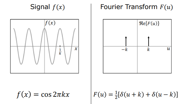
6.2 Sum of Cosines
A signal composed of two cosines $f(x) = \cos(2\pi k_1 x) + \cos(2\pi k_2 x)$ produces four delta impulses located at $u = \pm k_1$ and $u = \pm k_2$.
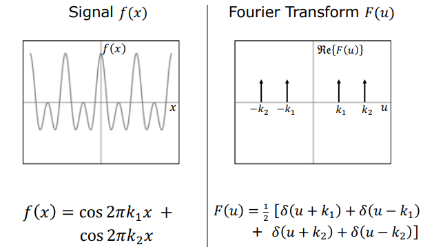
6.3 Sine Function
$f(x) = \sin(2\pi k x)$ also contains frequency $k$, but its delta impulses lie on the imaginary axis with opposite signs:
$$\mathcal{F}{\sin(2\pi k x)} = \frac{i}{2} \left[ \delta(u + k) - \delta(u - k) \right]$$
6.4 Constant Function
A constant DC signal $f(x) = 1$ has zero spatial variation (zero frequency). Its spectrum is a single Dirac impulse at the origin $u = 0$:
$$\mathcal{F}{1} = \delta(u)$$
6.5 Unit Impulse (Dirac Delta) Function
A point impulse $f(x) = \delta(x)$ requires equal contributions across all frequencies to form its infinite spatial spike. Its Fourier transform is completely flat:
$$\mathcal{F}{\delta(x)} = 1$$
6.6 Rectangular Window Function
A spatial boxcar / rectangle function $f(x) = \text{Rect}(x/T)$ of width $T$ transforms into a Sinc function:
$$\mathcal{F}{\text{Rect}(x/T)} = T \cdot \text{sinc}(Tu) = T \frac{\sin(\pi T u)}{\pi T u}$$
6.7 Gaussian Function
A spatial Gaussian $f(x) = e^{-ax^2}$ with variance parameter $a$ transforms into another Gaussian in the frequency domain:
$$\mathcal{F}{e^{-ax^2}} = \sqrt{\frac{\pi}{a}} e^{-\frac{\pi^2 u^2}{a}}$$
6.8 Inverse Scaling Principle
As demonstrated by the Gaussian and Rect-Sinc pairs, stretching a signal spatially causes it to contract in the frequency domain, and vice versa:
$$f(ax) \iff \frac{1}{|a|} F\left(\frac{u}{a}\right)$$
7. Fundamental Properties of Fourier Transform
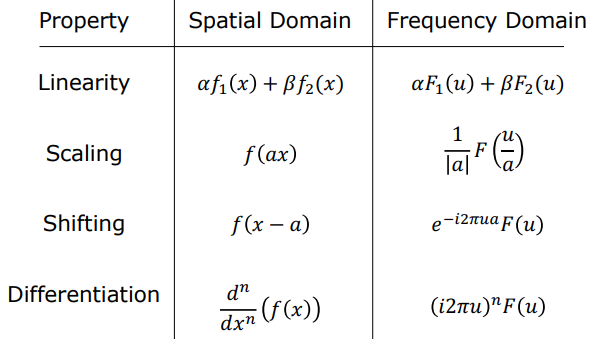
| Property | Spatial Domain ($f(x)$) | Frequency Domain ($F(u)$) | Technical Description |
|---|---|---|---|
| Linearity | $\alpha f_1(x) + \beta f_2(x)$ | $\alpha F_1(u) + \beta F_2(u)$ | Superposition and scaling principles hold in both domains. |
| Scaling | $f(ax)$ | $\frac{1}{|a|} F\left(\frac{u}{a}\right)$ | Spatial expansion causes frequency compression. |
| Shifting | $f(x - a)$ | $F(u) e^{-i 2\pi u a}$ | Spatial translation alters phase without affecting magnitude. |
| Differentiation | $\frac{d^n f(x)}{dx^n}$ | $(i 2\pi u)^n F(u)$ | Taking spatial derivatives amplifies high frequencies (sharpening). |
8. Convolution Theorem
Continuous 1D spatial convolution ($*$) between an image signal $f(x)$ and a system filter $h(x)$ is defined as:
$$g(x) = f(x) * h(x) = \int_{-\infty}^{\infty} f(\tau) h(x - \tau) , d\tau$$
Graphically, spatial convolution involves flipping the filter kernel $h(\tau) \to h(-\tau)$, shifting it by offset $x$, multiplying by $f(\tau)$, and integrating the overlapping area. For example, convolving two identical rectangular boxcars produces a symmetric triangle function.
8.1 Theorem Statement
The Convolution Theorem links spatial operations to frequency operations:
$$\mathcal{F}{f(x) * h(x)} = F(u) \cdot H(u)$$
$$\mathcal{F}{f(x) \cdot h(x)} = F(u) * H(u)$$
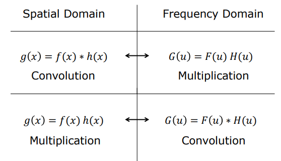
- Spatial Convolution $\iff$ Frequency Multiplication: Convolving two signals in space is equivalent to point-wise multiplying their Fourier transforms in frequency.
- Spatial Multiplication $\iff$ Frequency Convolution: Point-wise multiplying two signals in space is equivalent to convolving their Fourier transforms in frequency.
8.2 Mathematical Proof of Convolution Theorem
We evaluate the Fourier transform $G(u)$ of the spatial convolution output $g(x) = f(x) * h(x)$:
$$G(u) = \int_{-\infty}^{\infty} g(x) e^{-i 2\pi u x} , dx$$
Substitute the spatial convolution integral into $g(x)$:
$$G(u) = \int_{-\infty}^{\infty} \left[ \int_{-\infty}^{\infty} f(\tau) h(x - \tau) , d\tau \right] e^{-i 2\pi u x} , dx$$
Exchange integration order and expand the complex exponential by introducing $+u\tau - u\tau$:
$$e^{-i 2\pi u x} = e^{-i 2\pi u (x - \tau)} e^{-i 2\pi u \tau}$$
Reorganizing the inner and outer integrals:
$$G(u) = \int_{-\infty}^{\infty} f(\tau) e^{-i 2\pi u \tau} \left[ \int_{-\infty}^{\infty} h(x - \tau) e^{-i 2\pi u (x - \tau)} , dx \right] d\tau$$
Apply change of variables $y = x - \tau$ (hence $dy = dx$). Because $\tau$ is finite, integration limits remain $[-\infty, \infty]$:
$$G(u) = \left( \int_{-\infty}^{\infty} f(\tau) e^{-i 2\pi u \tau} , d\tau \right) \cdot \left( \int_{-\infty}^{\infty} h(y) e^{-i 2\pi u y} , dy \right)$$
The first integral is the exact definition of $F(u)$, and the second integral is $H(u)$:
$$G(u) = F(u) \cdot H(u) \quad \blacksquare$$
8.3 Computational Efficiency and Engineering Impact
Convolving an $N \times N$ image with a large spatial filter kernel has $O(N^2)$ computational complexity per pixel. By leveraging the Convolution Theorem and the Fast Fourier Transform (FFT):
flowchart LR
F_space["Spatial Signals <br/> f(x), h(x)"] -->|"FFT"| F_freq["Spectra <br/> F(u), H(u)"]
F_freq -->|"Multiply: F(u) · H(u)"| G_freq["Output Spectrum <br/> G(u)"]
G_freq -->|"IFFT"| G_space["Output Image <br/> g(x)"]
style F_space fill:#1a1a2e,stroke:#e94560,color:#fff
style F_freq fill:#16213e,stroke:#0f3460,color:#fff
style G_freq fill:#0f3460,stroke:#e94560,color:#fff
style G_space fill:#16213e,stroke:#4cc9f0,color:#fff
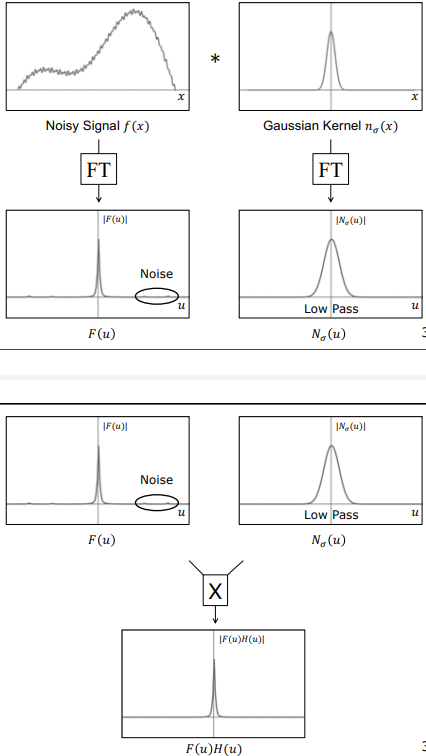
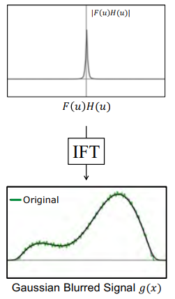
- Compute $F(u) = \mathcal{F}{f(x)}$ and $H(u) = \mathcal{F}{h(x)}$ using FFT ($O(N \log N)$).
- Perform element-wise multiplication $G(u) = F(u) \cdot H(u)$ ($O(N)$).
- Compute the Inverse FFT $g(x) = \mathcal{F}^{-1}{G(u)}$ ($O(N \log N)$).
This reduces computational complexity from $O(N^2)$ to $O(N \log N)$, providing enormous acceleration for large filter kernels and offering clear visual insight into which spatial frequencies a filter attenuates or passes.
Filtering in Frequency Domain and Deconvolution
- 1. Two-Dimensional (2D) Fourier Transform
- 2. Visualizing the 2D Frequency Spectrum
- 3. 2D Spectrum Examples & Physical Interpretations
- 4. Fundamental Image Filters in Frequency Domain
- 5. Critical Importance of Phase Information
- 6. Hybrid Images
- 7. Deblurring and Deconvolution
- 8. Wiener Deconvolution
1. Two-Dimensional (2D) Fourier Transform
Because images are two-dimensional spatial intensity distributions $f(x,y)$, the 1D Fourier Transform equations are extended to incorporate both horizontal ($u$) and vertical ($v$) spatial frequency components.
flowchart TD
A["2D Spatial Image <br/> f(x,y)"] -->|"2D Fourier Transform"| B["2D Frequency Spectrum <br/> F(u,v)"]
B -->|"Phase Spectrum ϕ(u,v) <br/> Spatial Structure"| C["Spatial Alignment"]
B -->|"Magnitude Spectrum |F(u,v)| <br/> Energy Distribution"| D["Logarithmic Compression <br/> log(1 + |F|)"]
style A fill:#1a1a2e,stroke:#e94560,color:#fff
style B fill:#16213e,stroke:#0f3460,color:#fff
style C fill:#0f3460,stroke:#e94560,color:#fff
style D fill:#0f3460,stroke:#4cc9f0,color:#fff
1.1 2D Continuous Fourier Transform (2D FT)
For a continuous 2D image function $f(x,y)$, the forward 2D Fourier Transform is defined as:
$$F(u,v) = \int_{-\infty}^{\infty} \int_{-\infty}^{\infty} f(x,y) e^{-i 2\pi (ux + vy)} , dx , dy$$
1.2 2D Inverse Continuous Fourier Transform (2D IFT)
The original continuous image $f(x,y)$ is reconstructed from its frequency spectrum $F(u,v)$ via:
$$f(x,y) = \int_{-\infty}^{\infty} \int_{-\infty}^{\infty} F(u,v) e^{i 2\pi (ux + vy)} , du , dv$$
1.3 2D Discrete Fourier Transform (2D DFT)
In digital computers, images consist of discrete $M \times N$ pixel matrices. Continuous integrals are transformed into double finite summations. Let $m, n$ denote spatial pixel indices ($0 \le m < M, 0 \le n < N$) and $p, q$ denote discrete frequency indices:
$$F[p,q] = \sum_{m=0}^{M-1} \sum_{n=0}^{N-1} f[m,n] e^{-i 2\pi \left(\frac{pm}{M} + \frac{qn}{N}\right)}$$
1.4 2D Inverse Discrete Fourier Transform (2D IDFT)
The discrete spatial image $f[m,n]$ is reconstructed from discrete frequency coefficients $F[p,q]$ via:
$$f[m,n] = \frac{1}{MN} \sum_{p=0}^{M-1} \sum_{q=0}^{N-1} F[p,q] e^{i 2\pi \left(\frac{pm}{M} + \frac{qn}{N}\right)}$$
2. Visualizing the 2D Frequency Spectrum
Because Fourier coefficients $F(u,v)$ are complex numbers, standard visual display discards the phase component and focuses on the magnitude spectrum $|F(u,v)|$.
2.1 Logarithmic Dynamic Range Compression
Magnitude values in an image spectrum often span several orders of magnitude (e.g., from $10^0$ to $10^6$). Displaying raw magnitude values directly renders small high-frequency details invisible. To visualize details across the dynamic range, logarithmic compression is applied:
$$D(u,v) = c \cdot \log(1 + |F(u,v)|)$$
where $c$ is a normalization scaling constant.
2.2 Spectrum Centering (FFT Shift)
By default, the zero-frequency component $F[0,0]$ resides at the top-left corner of the spectrum matrix. For intuitive interpretation, an FFT shift operation rotates quadrant origins to place $(u=0, v=0)$ directly at the geometric center of the spectrum display. Higher spatial frequencies extend radially outward from the center.
2.3 The DC Component
Because digital image intensity values cannot be negative (e.g., 8-bit intensities range from 0 to 255), images have a non-zero average brightness. The central coefficient $F(0,0)$—termed the DC component (Direct Current)—represents total average image brightness and appears as a prominent bright spot at the spectrum center:
$$F(0,0) = \sum_{m=0}^{M-1} \sum_{n=0}^{N-1} f[m,n]$$
3. 2D Spectrum Examples & Physical Interpretations
The orientation and spatial distribution of structures in an image map directly to specific patterns in its 2D Fourier magnitude spectrum:
- Horizontal Cosine Wave: A pure horizontal sinusoid produces a central DC spot plus two symmetric impulses located along the horizontal frequency axis at $\pm k$. Summing two cosines generates 5 spectral spots.
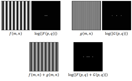
- Slit / Rectangular Window & Disk: A slanted rectangular aperture generates orthogonal high-frequency lines, while a circular disk yields a rotationally symmetric Airy-like spectrum.
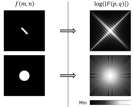
- Rubik’s Cube & Mandrill Texture: Images dominated by distinct edge directions generate bright radial rays, whereas complex natural textures produce a diffuse spectral cloud.
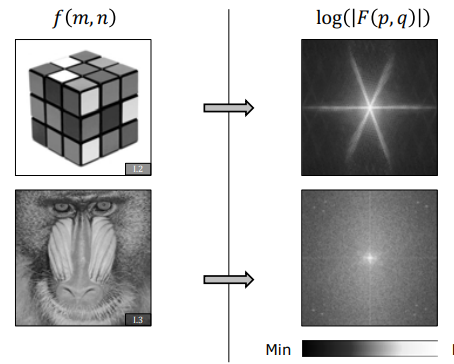
- Random Noise: Noise consists of rapid, uncorrelated spatial fluctuations. It produces a uniform, wideband energy distribution spread evenly across the entire frequency spectrum.
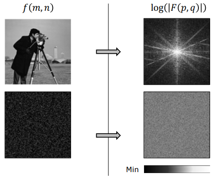
4. Fundamental Image Filters in Frequency Domain
Frequency domain filtering modifies an image by multiplying its Fourier spectrum $F(u,v)$ by a frequency transfer function $H(u,v)$:
$$G(u,v) = F(u,v) \cdot H(u,v)$$
flowchart LR
F["Input Spectrum <br/> F(u,v)"] --> LPF["Low-Pass Filter <br/> Attenuates High Freqs"] --> Blur["Smooth / Blurred Image"]
F --> HPF["High-Pass Filter <br/> Attenuates Low Freqs"] --> Edge["Edge / Contour Map"]
F --> Gauss["Gaussian Filter <br/> Smooth Transition"] --> Clean["Artifact-Free Blur"]
style F fill:#1a1a2e,stroke:#e94560,color:#fff
style LPF fill:#16213e,stroke:#0f3460,color:#fff
style HPF fill:#16213e,stroke:#0f3460,color:#fff
style Gauss fill:#0f3460,stroke:#4cc9f0,color:#fff
4.1 Low-Pass Filter (LPF)
A Low-Pass Filter suppresses high frequencies beyond a cutoff distance $D_0$ while preserving central low frequencies:
$$H_{\text{ILPF}}(u,v) = \begin{cases} 1 & \text{if } D(u,v) \le D_0 \ 0 & \text{if } D(u,v) > D_0 \end{cases}$$
- Visual Output: Smooths noise and fine textures, producing a blurred image.
- Radius Effect: Decreasing the cutoff radius $D_0$ blocks more high frequencies, resulting in progressively heavier blurring.
- Ideal Filter Artifacts: Using a sharp step cutoff (Ideal LPF) causes spatial ringing artifacts (Gibbs phenomenon) and blocky patterns due to the spatial Sinc footprint of the sharp frequency boundary.
4.2 High-Pass Filter (HPF)
A High-Pass Filter suppresses low frequencies (including the central DC component) while passing high frequencies:
$$H_{\text{IHPF}}(u,v) = 1 - H_{\text{ILPF}}(u,v)$$
- Visual Output: Homogeneous background regions turn black, isolating sharp intensity transitions, edges, and fine details.
- Computer Vision Role & Radius Effect: Fundamental edge and corner detection operators (e.g., Sobel, Laplacian) act as high-pass filters. Increasing the cutoff radius refines and sharpens extracted edge lines.
4.3 Gaussian Smoothing
To eliminate ringing artifacts caused by ideal step filters, a Gaussian Low-Pass Filter (GLPF) employs a smooth, continuous exponential decay:
$$H_{\text{GLPF}}(u,v) = e^{-\frac{D^2(u,v)}{2 D_0^2}}$$
By the Convolution Theorem, multiplying by a Gaussian in the frequency domain is equivalent to convolving with a spatial Gaussian kernel.
- Inverse Scaling Effect: As the spatial Gaussian mask is widened, the frequency Gaussian narrows, attenuating more high frequencies and producing heavier blur.
5. Critical Importance of Phase Information
While the magnitude spectrum $|F(u,v)|$ indicates how much energy exists at each frequency, the phase spectrum $\phi(u,v)$ specifies where those frequency components align in spatial coordinates.
Key Insight: Phase Preserves Structural Identity
Pioneering experiments by Oppenheim, Lim, and Curtis (1983) demonstrated that spatial structure and visual identity are governed predominantly by phase, not magnitude.
5.1 The Phase vs. Magnitude Experiment
- Magnitude-Only Reconstruction: If the phase spectrum of a portrait (Marilyn Monroe or Albert Einstein) is set to zero while keeping its original magnitude spectrum, the reconstructed inverse Fourier image becomes an unrecognizable, diffuse, cloud-like blob.
- Phase-Only Reconstruction with Swapped Magnitude: If the original phase spectrum of Marilyn Monroe is combined with the magnitude spectrum of an entirely unrelated scene (e.g., a landscape), the inverse Fourier transform clearly displays the sharp facial contours and recognizable identity of Marilyn Monroe.
flowchart TD
PhaseA["Portrait A Phase <br/> ϕ_A(u,v)"] --> Combine["+ (Combine Phase & Mag)"]
MagB["Portrait B Magnitude <br/> |F_B(u,v)|"] --> Combine
Combine --> IFT["Inverse Fourier Transform"]
IFT --> Out["Reconstructed Image <br/> Shows Portrait A Features!"]
style PhaseA fill:#1a1a2e,stroke:#e94560,color:#fff
style MagB fill:#16213e,stroke:#0f3460,color:#fff
style Combine fill:#0f3460,stroke:#e94560,color:#fff
style IFT fill:#16213e,stroke:#4cc9f0,color:#fff
style Out fill:#0f3460,stroke:#4cc9f0,color:#fff
6. Hybrid Images
Developed by Aude Oliva (2006), Hybrid Images exploit human visual perception and the spatial Point Spread Function (PSF) of the human eye to create optical illusions that change depending on viewing distance.
flowchart LR
Img1["Image 1 <br/> Einstein"] --> HPF["High-Pass Filter <br/> Fine Details"] --> Sum["Add Images"]
Img2["Image 2 <br/> Marilyn"] --> LPF["Low-Pass Filter <br/> Smooth Shapes"] --> Sum
Sum --> Hybrid["Hybrid Image"]
Hybrid --> Near["Close Distance: <br/> High Freq Dominates (Einstein)"]
Hybrid --> Far["Far Distance: <br/> Eye PSF Filters High Freq (Marilyn)"]
style Img1 fill:#1a1a2e,stroke:#e94560,color:#fff
style Img2 fill:#1a1a2e,stroke:#e94560,color:#fff
style Sum fill:#16213e,stroke:#0f3460,color:#fff
style Hybrid fill:#0f3460,stroke:#e94560,color:#fff
style Near fill:#16213e,stroke:#4cc9f0,color:#fff
style Far fill:#16213e,stroke:#4cc9f0,color:#fff
6.1 Construction Pipeline
- High-Pass Component: Apply a High-Pass Filter to an image (Albert Einstein) to extract sharp edge details.
- Low-Pass Component: Apply a Low-Pass Filter to a second image (Marilyn Monroe) to extract smooth background shading.
- Superposition: Sum the two filtered images to produce a single Hybrid Image.
6.2 Perceptual Mechanism
- Close Viewing Distance: High spatial frequencies are resolved sharply by the retina, causing the observer to perceive the high-pass image (Einstein).
- Far Viewing Distance: The angular resolution and defocus PSF of the human eye attenuate high spatial frequencies, leaving only the low-frequency component (Marilyn Monroe).
7. Deblurring and Deconvolution
During image acquisition, camera motion or defocus blurs an ideal sharp scene $f(x,y)$ via spatial convolution with a degradation function $h(x,y)$ (the Point Spread Function or PSF):
$$g(x,y) = f(x,y) * h(x,y)$$
Deconvolution is the process of reversing this spatial degradation to recover the unblurred scene $f(x,y)$.
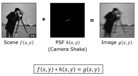
7.1 PSF Estimation via Inertial Measurement Units (IMU)
In modern smartphone cameras, physical camera shake $h(x,y)$ is estimated using hardware IMU sensors (accelerometers and gyroscopes). By tracking 3D camera rotation and translation during sensor exposure, the exact motion blur kernel $h(x,y)$ is calculated mathematically.
7.2 Naïve Inverse Filtering and Its Collapse
In an ideal noise-free environment, transforming $g(x,y) = f(x,y) * h(x,y)$ into the frequency domain yields:
$$G(u,v) = F(u,v) \cdot H(u,v) \implies F’(u,v) = \frac{G(u,v)}{H(u,v)}$$
Taking the Inverse Fourier Transform $\text{IFT}{F’(u,v)}$ recovers $f(x,y)$ perfectly.
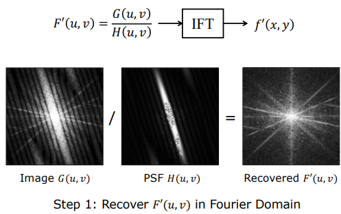
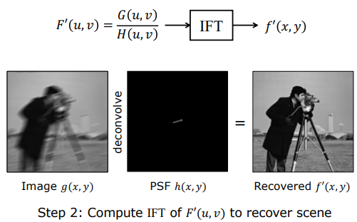
However, all real sensor systems introduce additive noise $n(x,y)$ (photon shot noise, thermal noise, quantization noise):
$$g(x,y) = f(x,y) * h(x,y) + n(x,y) \implies G(u,v) = F(u,v)H(u,v) + N(u,v)$$
Applying naïve inverse filtering to this realistic model yields:
$$F’(u,v) = \frac{G(u,v)}{H(u,v)} = F(u,v) + \frac{N(u,v)}{H(u,v)}$$
Warning: Double Mathematical Failure of Simple Inverse Filtering
- Division by Zero: Motion blur kernels $H(u,v)$ act as low-pass filters whose frequency values drop to zero at higher frequencies. Evaluating $\frac{1}{H(u,v)}$ at these zeros causes division-by-zero singularities ($\infty$).
- Severe Noise Amplification: At high frequencies where $|H(u,v)| \approx 0$, non-zero noise components $N(u,v)$ are multiplied by massive numbers ($\frac{N}{H} \gg 1$). The noise term completely overwhelms the true signal $F(u,v)$, corrupting the restored image with extreme salt-and-pepper noise artifacts.
8. Wiener Deconvolution
To prevent noise amplification and safely invert degraded signals, Wiener Deconvolution incorporates a dynamic frequency weighting factor based on signal and noise power.
flowchart TD
Degradation["Blurred & Noisy Spectrum <br/> G(u,v) = F·H + N"] --> Wiener["Wiener Filter <br/> 1/H · [|H|² / (|H|² + NSR)]"]
Wiener --> Reconstructed["Restored Spectrum <br/> F'(u,v)"]
Reconstructed --> IFT["Inverse FFT"] --> Output["Clean Sharp Image"]
style Degradation fill:#1a1a2e,stroke:#e94560,color:#fff
style Wiener fill:#16213e,stroke:#0f3460,color:#fff
style Reconstructed fill:#0f3460,stroke:#e94560,color:#fff
style Output fill:#16213e,stroke:#4cc9f0,color:#fff
8.1 Theoretical Wiener Filter Formula
The theoretical Wiener filter minimizes the mean square error between the estimated image $f’(x,y)$ and the true image $f(x,y)$:
$$F’(u,v) = \frac{G(u,v)}{H(u,v)} \cdot \left[ \frac{1}{1 + \frac{\text{NSR}(u,v)}{|H(u,v)|^2}} \right]$$
where $\text{NSR}(u,v)$ represents the spectral Noise-to-Signal Ratio:
$$\text{NSR}(u,v) = \frac{|N(u,v)|^2}{|F(u,v)|^2}$$
8.2 Working Mechanism
- High-SNR Frequencies ($|N|^2 \ll |F|^2$): $\text{NSR} \to 0$, making the bracketed term approach $1$. The filter acts as a standard inverse filter $\frac{G}{H}$.
- Low-SNR / High-Noise Frequencies ($|H| \to 0$ or $|N|^2 \gg |F|^2$): $\frac{\text{NSR}}{|H|^2} \to \infty$, driving the bracketed weighting term to $0$. This safely suppresses high-frequency noise amplification and avoids division by zero.
8.3 Practical Constant $\lambda$ Approximation
Because true noise $|N(u,v)|^2$ and unblurred scene spectra $|F(u,v)|^2$ are rarely known prior to restoration, practical implementations approximate NSR using a small user-defined constant parameter $\lambda$ (e.g., $\lambda \approx 0.002$):
$$F’(u,v) = \frac{G(u,v)}{H(u,v)} \cdot \left[ \frac{|H(u,v)|^2}{|H(u,v)|^2 + \lambda} \right]$$
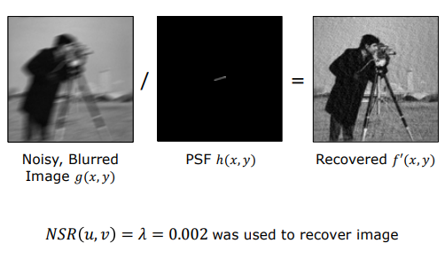
While choosing a fixed $\lambda$ may leave minor ringing artifacts near sharp boundaries, Wiener deconvolution dramatically sharpens blurred, noisy images into clear, visually crisp results.
Sampling Theory and Aliasing
- 1. Digitization and the Sampling Problem
- 2. Mathematical Model of Sampling (Shah Function)
- 3. Nyquist-Shannon Sampling Theorem
- 4. Signal Reconstruction (Perfect Recovery)
- 5. Anti-Aliasing Techniques
1. Digitization and the Sampling Problem
Converting a continuous physical scene into a digital image requires spatial sampling—discretizing continuous space into a grid of pixel intensity samples. This poses a fundamental engineering question: How densely must we place pixels to preserve all visual information from a continuous scene without any loss?
flowchart TD
A["Continuous Physical Scene <br/> f(x)"] --> B["Spatial Sampling <br/> Spacing x_0"]
B -->|"Well-Sampled: u_max ≤ 1 / (2 x_0)"| C["Perfect Reconstruction <br/> No Information Loss"]
B -->|"Under-Sampled: u_max > 1 / (2 x_0)"| D["Aliasing Artifacts <br/> Moiré Patterns"]
style A fill:#1a1a2e,stroke:#e94560,color:#fff
style B fill:#16213e,stroke:#0f3460,color:#fff
style C fill:#0f3460,stroke:#4cc9f0,color:#fff
style D fill:#0f3460,stroke:#e94560,color:#fff
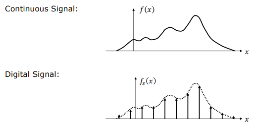
1.1 Under-Sampling and Information Loss
If a high-frequency continuous signal (a fast-oscillating sinusoid) is sampled too coarsely:
- Connecting the discrete sample points via linear interpolation produces either a completely flat line or an entirely spurious low-frequency sinusoid that never existed in the original continuous scene.
- The creation of false, low-frequency artifacts caused by inadequate spatial sampling is called Aliasing.
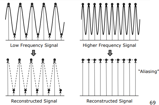
1.2 Visual Manifestation: Moiré Patterns
In digital photography and computer vision, aliasing manifests visually as Moiré Patterns—spurious wavy bands, ripples, or rainbow halos appearing on fine repetitive structures such as brick walls, pinstriped shirts, or tight radial grids.
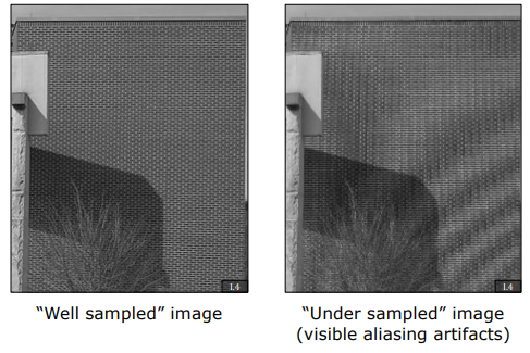
2. Mathematical Model of Sampling (Shah Function)
Mathematically, sampling a continuous 1D signal $f(x)$ at regular spatial intervals $x_0$ is modeled as multiplying $f(x)$ by an infinite train of Dirac delta functions, known as the Shah Function (or impulse train) $s(x)$.
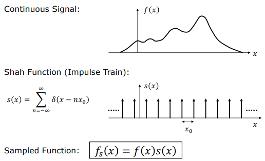
$$s(x) = \sum_{n=-\infty}^{\infty} \delta(x - n x_0)$$
The sampled signal $f_s(x)$ is defined as:
$$f_s(x) = f(x) \cdot s(x) = f(x) \sum_{n=-\infty}^{\infty} \delta(x - n x_0)$$
2.1 Fourier Transform of the Shah Function
The Fourier Transform of a spatial Shah function with period $x_0$ is another Shah function in the frequency domain with spacing $\frac{1}{x_0}$:
$$\mathcal{F}{s(x)} = S(u) = \frac{1}{x_0} \sum_{n=-\infty}^{\infty} \delta\left(u - \frac{n}{x_0}\right)$$
2.2 Sampling in Frequency Domain (Convolution Theorem)
By the Convolution Theorem, multiplication in the spatial domain corresponds to convolution in the frequency domain:
$$\mathcal{F}{f_s(x)} = F_s(u) = F(u) * S(u)$$
$$F_s(u) = F(u) * \left[ \frac{1}{x_0} \sum_{n=-\infty}^{\infty} \delta\left(u - \frac{n}{x_0}\right) \right] = \frac{1}{x_0} \sum_{n=-\infty}^{\infty} F\left(u - \frac{n}{x_0}\right)$$
Key Insight: Periodic Spectrum Replication
Spatial sampling replicates the original continuous frequency spectrum $F(u)$ infinitely along the frequency axis at steps of $\frac{1}{x_0}$.
3. Nyquist-Shannon Sampling Theorem
The fundamental cornerstone of digital signal processing and computer vision—the Nyquist-Shannon Sampling Theorem—defines the exact condition required for perfect signal reconstruction without information loss.
flowchart LR
Cont["Continuous Signal <br/> Max Frequency u_max"] --> Cond{"Nyquist Condition: <br/> u_max ≤ 1 / (2 x_0)"}
Cond -->|Yes| Safe["Non-Overlapping Spectra <br/> Low-Pass Filter <br/> Perfect Reconstruction"]
Cond -->|No| Alias["Overlapping Spectra <br/> Distorted Original Signal <br/> Irreversible Information Loss!"]
style Cont fill:#1a1a2e,stroke:#e94560,color:#fff
style Cond fill:#16213e,stroke:#0f3460,color:#fff
style Safe fill:#0f3460,stroke:#4cc9f0,color:#fff
style Alias fill:#0f3460,stroke:#e94560,color:#fff
3.1 Theorem Statement
To recover a band-limited continuous signal with maximum frequency $u_{\max}$ without error, the spatial sampling interval $x_0$ must satisfy:
$$u_{\max} \le \frac{1}{2 x_0} \quad \iff \quad \frac{1}{x_0} \ge 2 u_{\max}$$
- Nyquist Frequency ($u_N = \frac{1}{2x_0}$): The maximum spatial frequency that can be represented unambiguously by a pixel grid of spacing $x_0$.
- Nyquist Rate ($2 u_{\max}$): The minimum sampling frequency required to digitize a continuous signal losslessly.
3.2 Spectral Overlapping (Aliasing in Frequency Domain)
If sampling is inadequate ($u_{\max} > \frac{1}{2x_0}$), adjacent spectral replicas spaced by $\frac{1}{x_0}$ overlap.
High-frequency components fold back across the Nyquist frequency boundary and masquerade as false low-frequency energy. Once aliasing occurs, isolating the original spectrum $F(u)$ becomes mathematically impossible.
4. Signal Reconstruction (Perfect Recovery)
When the Nyquist condition is met ($u_{\max} \le \frac{1}{2x_0}$), the original spectrum $F(u)$ is isolated from periodic replicas $F_s(u)$ using an ideal Low-Pass Reconstruction Filter $C(u)$ (a boxcar function):
$$C(u) = \begin{cases} x_0 & \text{if } |u| < \frac{1}{2x_0} \ 0 & \text{otherwise} \end{cases}$$
$$F(u) = F_s(u) \cdot C(u)$$
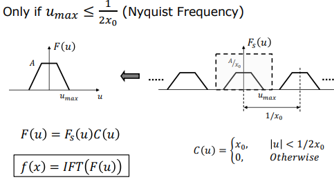
In the spatial domain, the frequency boxcar function $C(u)$ corresponds to a Sinc function:
$$c(x) = \mathcal{F}^{-1}{C(u)} = \text{sinc}\left(\frac{x}{x_0}\right)$$
$$f(x) = f_s(x) * c(x) = \sum_{n=-\infty}^{\infty} f(n x_0) \cdot \text{sinc}\left(\frac{x - n x_0}{x_0}\right)$$
This formula (the Whittaker-Shannon Interpolation Formula) proves that a continuous signal can be reconstructed perfectly from discrete samples using Sinc Interpolation.
5. Anti-Aliasing Techniques
Real-world optical scenes contain sharp boundaries and fine textures with infinitely high frequency components. Thus, no physical image sensor can satisfy the strict Nyquist condition natively without pre-filtering.
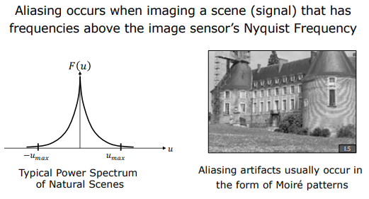
Digital camera systems employ two hardware strategies to prevent aliasing:
5.1 Physical Sensor Strategies
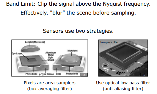
- Pixel Integration Area (Box-Averaging Filter): Sensor pixels are non-zero area photodiodes rather than mathematical point samplers. Light hitting a pixel surface is integrated over its finite area, acting as a spatial box filter that naturally attenuates ultra-high frequencies.
- Optical Low-Pass Filter (OLPF / Anti-Aliasing Filter): A thin birefringent crystal layer positioned directly in front of the image sensor. It blurs the incoming optical image slightly before light reaches the photodiode array. By attenuating spatial frequencies above the Nyquist limit ($u_N = \frac{1}{2x_0}$), it prevents the generation of Moiré artifacts.
Overview, Gradients, and Laplacian Edge Detection
- 1. Introduction and What is an Edge?
- 2. Edge Detection Using Gradients
- 3. Edge Detection Using Laplacian
- 4. Comparison of Gradient and Laplacian Operators
This technical note covers one of the fundamental information theory topics in computer vision: Edge Detection. We explore its physical origins, mathematical formulations based on first derivatives (Gradients), and second derivatives (Laplacian), along with their practical discrete implementations.
1. Introduction and What is an Edge?
1.1. Definition of Edge and Information Theory Perspective
In computer vision, an edge is defined as a set of connected pixels in a local neighborhood across which the image intensity (brightness) undergoes a sharp, abrupt, and directional change.
flowchart LR
A["Raw Image\n(High Data Redundancy)"] --> B["Edge Extraction\n(Gradient / Laplacian)"]
B --> C["Sparse Contour Map\n(High Information Density)"]
style A fill:#1a1a2e,stroke:#16213e,color:#fff
style B fill:#0f3460,stroke:#e94560,color:#fff
style C fill:#16213e,stroke:#4cc9f0,color:#fff
From an information theory perspective, edges carry the vast majority of semantic and geometric information of a scene while discarding illumination variations and homogeneous regions:
- Data Sparsity: Retaining only edge pixels dramatically compresses the image payload, transforming dense pixel matrices into sparse structures.
- Perceptual Sufficiency: Human visual perception relies heavily on boundary contours. As demonstrated by Vic Nalwa using Henry Moore’s sculpture artwork, comparing a high-resolution photograph of a 3D sculpture with a minimal line sketch reveals that human visual cortex can reconstruct 3D shape, curvature, and surface highlights using almost exclusively sparse line contours.
Key Insight: Edges maximize information density by encoding 3D object geometry, surface boundaries, and illumination transitions while suppressing redundant homogeneous background data.
1.2. Physical Causes of Edges
Intensity discontinuities in the image plane stem from four fundamental physical phenomena in the 3D world:
flowchart TD
E["Physical Edge Causes"] --> D1["1. Depth Discontinuity"]
E --> D2["2. Surface Normal Discontinuity"]
E --> D3["3. Reflectance Discontinuity"]
E --> D4["4. Illumination Discontinuity"]
D1 --> C1["Object occluding background\n(Distance step)"]
D2 --> C2["Kink/corner between faces\n(Orientation change)"]
D3 --> C3["Albedo / material boundary\n(Paint, texture, markings)"]
D4 --> C4["Cast shadow boundaries\n(Light intensity change)"]
style E fill:#1a1a2e,stroke:#e94560,color:#fff
style D1 fill:#16213e,stroke:#4cc9f0,color:#fff
style D2 fill:#16213e,stroke:#4cc9f0,color:#fff
style D3 fill:#16213e,stroke:#4cc9f0,color:#fff
style D4 fill:#16213e,stroke:#4cc9f0,color:#fff
- Depth Discontinuity: Occurs when an object occludes another object or background, producing an abrupt step change in distance relative to the camera sensor.
- Surface Normal Discontinuity: Occurs at geometric boundaries where two surfaces meet at an angle (e.g., the edge of a cube). Even if both surfaces possess identical material properties, their distinct 3D orientations cause them to receive different amounts of incident light.
- Surface Reflectance Discontinuity: Occurs due to changes in surface material composition, paint, or albedo (e.g., printed text on a label, surface markings).
- Illumination / Shadow Discontinuity: Occurs at boundaries formed by cast shadows or specular highlights, where incident light intensity changes abruptly.
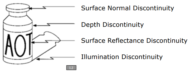
1.3. Edge Profile Types and Real-World Challenges
Mathematically, edge profiles are categorized into idealized 1D models:
- Step Edge: An instantaneous transition from intensity $I_0$ to $I_1$.
- Ramp / Step Edge with Gradient: A continuous, sloped intensity transition across a finite spatial width.
- Roof Edge / Line Edge: A thin ridge formed by two adjacent ramp transitions (a rising ramp immediately followed by a falling ramp).
$$\begin{aligned} \text{Step Edge:} \quad & f(x) = \begin{cases} I_0, & x < 0 \ I_1, & x \ge 0 \end{cases} \ \text{Roof Edge:} \quad & f(x) = \begin{cases} I_0 + k x, & x < 0 \ I_0 - k x, & x \ge 0 \end{cases} \end{aligned}$$
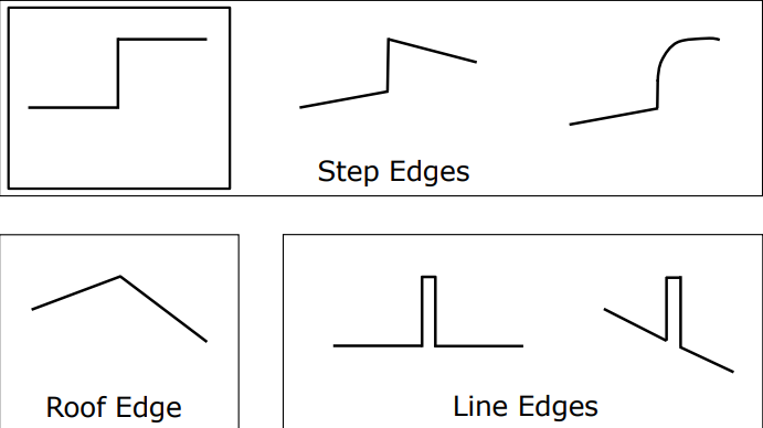
In real-world camera systems, ideal step edges do not exist due to physical degradation factors:
- Sensor noise (shot noise, thermal noise)
- Optical blur and point spread function (PSF) limitations
- Spatial discretization (sampling) and quantization noise
- Out-of-focus defocus blur
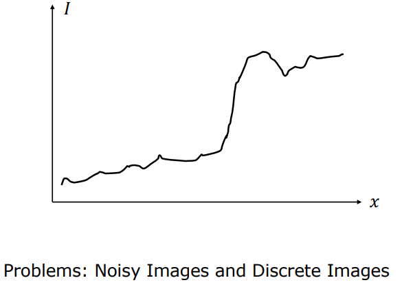
1.4. Criteria for an Ideal Edge Operator
An edge detection operator processes local pixel neighborhoods and must output three key measurements for every pixel:
- Edge Position: Precise pixel or sub-pixel spatial coordinates $(x, y)$.
- Edge Strength / Magnitude: The degree of intensity contrast.
- Edge Orientation: The normal direction angle $\theta$ relative to the horizontal axis.
John Canny formalized the optimal mathematical performance requirements for edge detectors into three criteria:
Canny’s Optimal Detection Criteria:
- High Detection Rate (Low Error Rate): Minimize false negatives (missing true edges) and false positives (marking noise as edges).
- Good Localization: The distance between the detected edge pixel and the true physical edge center must be minimized.
- Single Response Constraint: The operator must return only one response per single edge (preventing thick, multiple response bands).
2. Edge Detection Using Gradients
Gradient-based edge detection computes first-order spatial derivatives to detect high rates of intensity change.
2.1. 1D Signal Analysis
For a 1D continuous intensity function $f(x)$:
- The first derivative $\frac{df}{dx}$ produces a local maximum (positive peak) for a rising edge.
- For a falling edge, $\frac{df}{dx}$ yields a local minimum (negative valley).
- Taking the absolute value $\left| \frac{df}{dx} \right|$ converts both rising and falling transitions into positive peaks. The peak location indicates the edge center, and the peak height reflects the edge contrast strength.
$$\frac{df}{dx} = \lim_{\Delta x \to 0} \frac{f(x + \Delta x) - f(x)}{\Delta x}$$
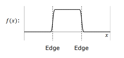
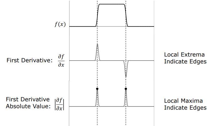
2.2. 2D Gradient Vector ($\nabla I$)
In 2D continuous space, intensity variations depend on direction. The Gradient Vector $\nabla I$ (or $\text{grad } I$) points in the direction of the steepest intensity increase:
$$\nabla I = \begin{bmatrix} \frac{\partial I}{\partial x} \[6pt] \frac{\partial I}{\partial y} \end{bmatrix} = \begin{bmatrix} I_x \[6pt] I_y \end{bmatrix}$$
From the partial derivatives $I_x$ and $I_y$, we compute two essential spatial metrics:
-
Gradient Magnitude (Edge Strength): $$|\nabla I| = \sqrt{I_x^2 + I_y^2} \approx |I_x| + |I_y|$$
-
Gradient Orientation (Normal Angle): $$\theta = \tan^{-1} \left( \frac{I_y}{I_x} \right)$$
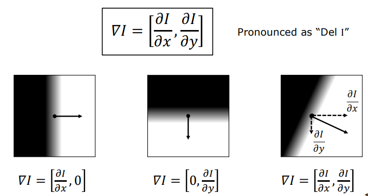
flowchart TD
Img["2D Image I(x,y)"] --> Ix["Compute Partial Derivative Ix"]
Img --> Iy["Compute Partial Derivative Iy"]
Ix --> Mag["Gradient Magnitude\n|∇I| = √(Ix² + Iy²)"]
Iy --> Mag
Ix --> Ang["Gradient Direction\nθ = arctan(Iy / Ix)"]
Iy --> Ang
style Img fill:#1a1a2e,stroke:#16213e,color:#fff
style Ix fill:#16213e,stroke:#4cc9f0,color:#fff
style Iy fill:#16213e,stroke:#4cc9f0,color:#fff
style Mag fill:#0f3460,stroke:#e94560,color:#fff
style Ang fill:#0f3460,stroke:#e94560,color:#fff
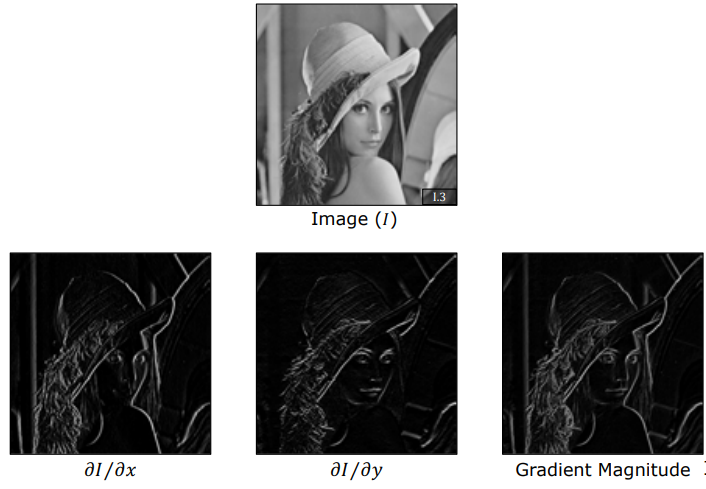
Note on Orientation: The gradient direction $\theta$ is perpendicular to the boundary contour of the edge. The actual tangent boundary line runs at an angle of $\theta + \frac{\pi}{2}$.
2.3. Finite Differences in Discrete Images
On a discrete 2D grid, continuous derivatives are approximated using finite differences. Using a symmetric center scheme requires small neighborhood windows:
$$\frac{\partial I}{\partial x} \approx \frac{I(x+1, y) - I(x-1, y)}{2\Delta x}, \quad \frac{\partial I}{\partial y} \approx \frac{I(x, y+1) - I(x, y-1)}{2\Delta y}$$
Assuming unit inter-pixel distance $\epsilon = 1$, 2D finite difference convolution kernels are expressed as:
$$M_x = \frac{1}{2} \begin{bmatrix} -1 & 1 \ -1 & 1 \end{bmatrix}, \quad M_y = \frac{1}{2} \begin{bmatrix} 1 & 1 \ -1 & -1 \end{bmatrix}$$
2.4. Comparison of Classic Gradient Filters
To mitigate high-frequency sensor noise, modern gradient operators combine a finite-difference derivative filter with a low-pass smoothing filter (e.g., Gaussian or uniform box filter).
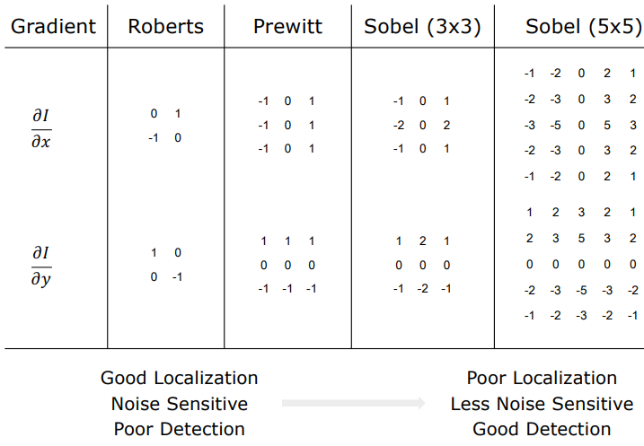
| Operator | Kernel Size | Mathematical Formulation | Properties & Trade-offs |
|---|---|---|---|
| Roberts Cross | $2 \times 2$ | $D_x = \begin{bmatrix} 0 & 1 \ -1 & 0 \end{bmatrix}, , D_y = \begin{bmatrix} 1 & 0 \ 0 & -1 \end{bmatrix}$ | Extremely fast, high localization accuracy, but highly sensitive to noise. |
| Prewitt | $3 \times 3$ | $P_x = \begin{bmatrix} -1 & 0 & 1 \ -1 & 0 & 1 \ -1 & 0 & 1 \end{bmatrix}, , P_y = \begin{bmatrix} 1 & 1 & 1 \ 0 & 0 & 0 \ -1 & -1 & -1 \end{bmatrix}$ | Combines 1D uniform smoothing with 1D central difference. Good noise attenuation. |
| Sobel | $3 \times 3$ | $S_x = \begin{bmatrix} -1 & 0 & 1 \ -2 & 0 & 2 \ -1 & 0 & 1 \end{bmatrix}, , S_y = \begin{bmatrix} 1 & 2 & 1 \ 0 & 0 & 0 \ -1 & -2 & -1 \end{bmatrix}$ | Weight of 2 at center pixel provides Gaussian smoothing. Industry standard $3 \times 3$ operator. |
| Extended Sobel | $5 \times 5+$ | Larger Gaussian-weighted derivative kernels | Excellent noise suppression, but degrades edge localization due to spatial blurring. |
2.5. Thresholding and Hysteresis
Once the gradient magnitude map $|\nabla I|$ is computed, binary edge maps are extracted via thresholding:
-
Single Global Thresholding: $$E(x,y) = \begin{cases} 1, & |\nabla I(x,y)| \ge T \ 0, & |\nabla I(x,y)| < T \end{cases}$$
- Problem: A high $T$ causes broken contours; a low $T$ introduces excessive false edges caused by noise.
-
Hysteresis Dual Thresholding: Uses two thresholds: a high threshold $T_{high}$ and a low threshold $T_{low}$.
- Strong Edges: $|\nabla I| \ge T_{high} \rightarrow$ Immediately accepted.
- Weak Edges: $T_{low} \le |\nabla I| < T_{high} \rightarrow$ Accepted only if connected to a strong edge path.
- Non-Edges: $|\nabla I| < T_{low} \rightarrow$ Rejected.
3. Edge Detection Using Laplacian
While gradient operators rely on first-order derivatives, the Laplacian approach uses second-order derivatives.
3.1. Second Derivative and Zero-Crossings
For a continuous 1D function $f(x)$, the second derivative $\frac{d^2f}{dx^2}$ measures acceleration in intensity change:
- At the inflection point (the exact center of a ramp edge), the second derivative passes through zero.
- The transition from positive peak to negative valley creates a sharp Zero-Crossing.
$$\frac{d^2f}{dx^2} = \lim_{\Delta x \to 0} \frac{f(x+\Delta x) - 2f(x) + f(x-\Delta x)}{\Delta x^2}$$
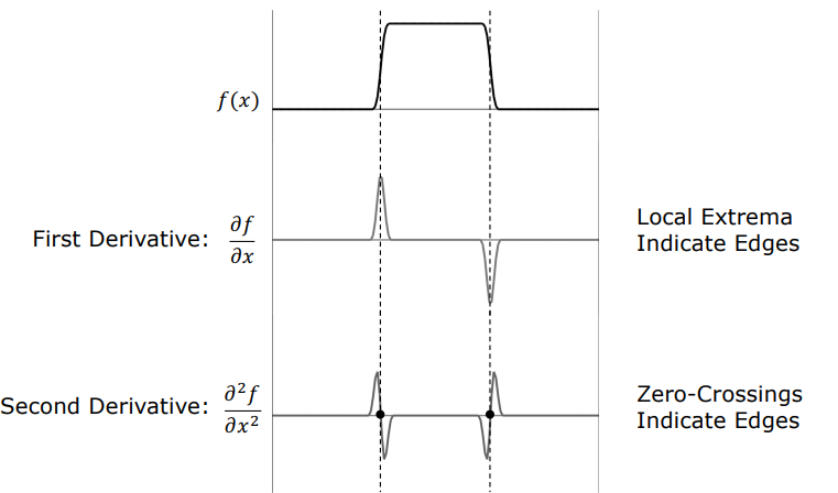
flowchart TD
Signal["Intensity Signal f(x)"] --> FirstDev["First Derivative df/dx\n(Peak at edge)"]
FirstDev --> SecDev["Second Derivative d²f/dx²\n(Zero-Crossing at edge center)"]
SecDev --> EdgeLoc["Detect Zero-Crossing\n(Sub-pixel Edge Location)"]
style Signal fill:#1a1a2e,stroke:#16213e,color:#fff
style FirstDev fill:#16213e,stroke:#4cc9f0,color:#fff
style SecDev fill:#0f3460,stroke:#e94560,color:#fff
style EdgeLoc fill:#0f3460,stroke:#e94560,color:#fff
Key Advantage: Finding local maxima of first derivatives is computationally sensitive to threshold choices, whereas finding zero-crossings of second derivatives provides precise, closed edge contours.
3.2. 2D Laplacian Operator ($\nabla^2 I$)
The 2D Laplacian operator is an isotropic (rotation-invariant) scalar operator defined as the sum of unmixed second partial derivatives:
$$\nabla^2 I = \frac{\partial^2 I}{\partial x^2} + \frac{\partial^2 I}{\partial y^2}$$
Key Properties:
- Isotropic: Responds equally to edges in all orientations.
- Scalar Output: Returns a single scalar response map rather than a vector.
- No Orientation Info: Unlike $\nabla I$, the Laplacian $\nabla^2 I$ does not provide the edge orientation angle $\theta$.
3.3. Discrete Laplacian Kernels and Diagonal Correction
In discrete grids, 2D second derivatives are approximated using 3x3 stencil operations:
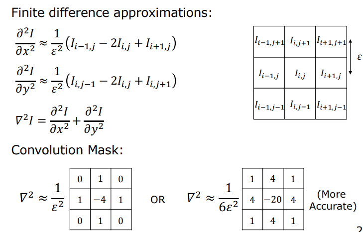
-
Standard 4-Neighbor Laplacian Kernel: $$L_4 = \begin{bmatrix} 0 & 1 & 0 \ 1 & -4 & 1 \ 0 & 1 & 0 \end{bmatrix}$$
-
Diagonal-Corrected 8-Neighbor Laplacian Kernel: To correct for spatial anisotropy along $45^\circ$ diagonal pixel distances ($\sqrt{2}\epsilon$), the weighted 8-neighbor stencil is preferred: $$L_8 = \begin{bmatrix} 1 & 4 & 1 \ 4 & -20 & 4 \ 1 & 4 & 1 \end{bmatrix}$$
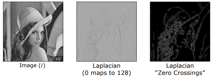
3.4. Noise Sensitivity and Solution: Gaussian Smoothing (LoG and DoG)
Second derivatives severely amplify high-frequency noise. Taking the second derivative of raw image noise yields unmanageable noise spikes.
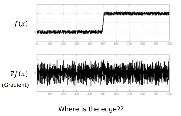
To solve this, the image must first be smoothed with a 2D Gaussian filter $G_\sigma(x,y)$:
$$G_\sigma(x,y) = \frac{1}{2\pi \sigma^2} e^{-\frac{x^2+y^2}{2\sigma^2}}$$
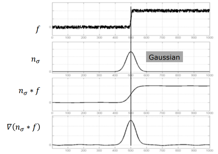
By the associative property of linear convolution:
$$\nabla^2 \left( G_\sigma * I \right) = \left( \nabla^2 G_\sigma \right) * I$$
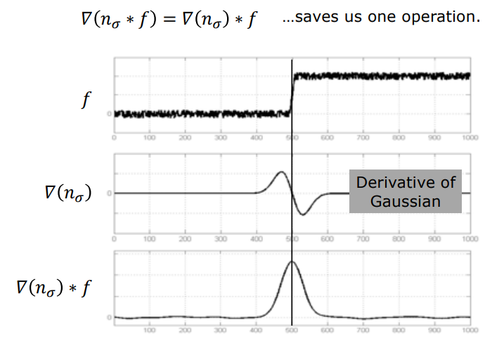
This leads to the Laplacian of Gaussian (LoG) operator (also known as the Mexican Hat Operator due to its 3D inverted shape):
$$\text{LoG}(x,y) = -\frac{1}{\pi \sigma^4} \left[ 1 - \frac{x^2+y^2}{2\sigma^2} \right] e^{-\frac{x^2+y^2}{2\sigma^2}}$$
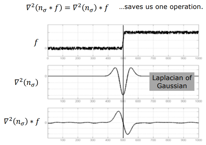
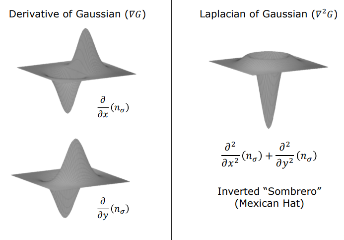
flowchart LR
Gaussian["Gaussian Filter G_σ"] --> LaplacianOp["Apply Laplacian ∇²"]
LaplacianOp --> LoGKernel["LoG Kernel (Mexican Hat)"]
LoGKernel --> Conv["Convolve with Image I"]
Conv --> ZeroCross["Zero-Crossing Detection"]
style Gaussian fill:#1a1a2e,stroke:#16213e,color:#fff
style LaplacianOp fill:#16213e,stroke:#4cc9f0,color:#fff
style LoGKernel fill:#0f3460,stroke:#e94560,color:#fff
style Conv fill:#0f3460,stroke:#e94560,color:#fff
style ZeroCross fill:#16213e,stroke:#4cc9f0,color:#fff
Alternatively, Difference of Gaussians (DoG) efficiently approximates LoG by subtracting two Gaussian-blurred images with slightly different scale factors $\sigma_1$ and $\sigma_2$:
$$\text{DoG}(x,y) = G_{\sigma_1}(x,y) - G_{\sigma_2}(x,y) \approx (\sigma_1 - \sigma_2) \nabla^2 G_\sigma$$
4. Comparison of Gradient and Laplacian Operators
The following matrix summarizes the fundamental trade-offs between Gradient-based and Laplacian-based edge detection techniques:
| Feature / Metric | Gradient Operator ($\nabla I$) | Laplacian Operator ($\nabla^2 I$ / LoG) |
|---|---|---|
| Mathematical Basis | First Derivative (Spatial Rate of Change) | Second Derivative (Inflection / Acceleration) |
| Primary Output | Edge Position, Magnitude $ | \nabla I |
| Edge Orientation ($\theta$) | Provided ($\theta = \arctan(I_y / I_x)$) | Not Provided (Isotropic / Rotationally Symmetric) |
| Linearity | Non-Linear (contains sqrt and arctan) | Linear (computed via linear matrix convolution) |
| Computational Complexity | Higher (requires 2 directional convolutions + nonlinear algebra) | Lower (single matrix convolution) |
| Detection Principle | Local Maxima Peak Detection + Thresholding | Zero-Crossing sign change detection |
| Noise Sensitivity | Moderate (mitigated by Sobel/Prewitt smoothing) | High (requires prior Gaussian filtering: LoG / DoG) |
Conclusion: Gradient operators provide direction and magnitude, making them essential for feature extraction and vector field computation. Laplacian operators provide mathematically continuous, closed zero-crossing boundaries. The fusion of these two methodologies led directly to the development of the Canny Edge Detector.
Canny Edge Detector and Corner Detection
- 1. Canny Edge Detector
- 2. Corner Detection (Harris & Moravec Corner Detector)
- 2.1. Why Corners? (2D Constraints & Aperture Problem)
- 2.2. Categorization of Image Neighborhoods
- 2.3. Mathematical Formulation (Sum of Squared Differences & Taylor Series)
- 2.4. Second Moment Matrix ($M$) and Eigenvalue Analysis
- 2.5. Harris Corner Response Function ($R$)
- 2.6. Complete Harris Corner Detection Pipeline
- 3. Summary Comparison of Edge vs Corner Detection
This technical note covers advanced feature extraction techniques in computer vision, focusing on the optimal Canny Edge Detector and Harris Corner Detection (Structure Tensor analysis). We examine their mathematical derivations, multi-scale behavior, spatial autocorrelation, eigenvalue analysis of second moment matrices, and practical algorithmic implementations.
1. Canny Edge Detector
The Canny Edge Detector, developed by John F. Canny in 1986, is widely regarded as the optimal edge detection algorithm for 2D images. It formulates edge detection as an analytical optimization problem subject to precise mathematical constraints.
1.1. John Canny’s Optimization Criteria
Canny defined three fundamental criteria that an optimal edge detector must satisfy:
- Low Error Rate (Optimal Detection): The operator must maximize the signal-to-noise ratio (SNR) by catching all true physical edges while minimizing false positives caused by noise.
- Localization Accuracy: The distance between the detected edge pixel coordinates and the true physical center of the edge boundary must be minimized.
- Single Response Constraint: The detector must return only one pixel-wide response for each single edge boundary, avoiding multiple thick response bands.
flowchart TD
Raw["Raw Input Image I(x,y)"] --> Step1["1. Gaussian Blur (G_σ * I)\n(Noise Suppression)"]
Step1 --> Step2["2. Gradient Calculation\n(|∇I| and Angle θ)"]
Step2 --> Step3["3. Non-Maximum Suppression (NMS)\n(Thinning Edges to 1-Pixel Width)"]
Step3 --> Step4["4. Hysteresis Dual Thresholding\n(High Thresh Th, Low Thresh Tl)"]
Step4 --> Step5["5. Edge Tracking by Connectivity\n(Connecting Weak Edges to Strong Edges)"]
Step5 --> Out["Final Binary Edge Map"]
style Raw fill:#1a1a2e,stroke:#16213e,color:#fff
style Step1 fill:#16213e,stroke:#4cc9f0,color:#fff
style Step2 fill:#16213e,stroke:#4cc9f0,color:#fff
style Step3 fill:#0f3460,stroke:#e94560,color:#fff
style Step4 fill:#0f3460,stroke:#e94560,color:#fff
style Step5 fill:#16213e,stroke:#4cc9f0,color:#fff
style Out fill:#1a1a2e,stroke:#4cc9f0,color:#fff
1.2. The 5-Step Canny Pipeline
Step 1: Gaussian Smoothing
To suppress high-frequency image noise, the raw image $I(x,y)$ is convolved with a 2D Gaussian kernel $G_\sigma(x,y)$:
$$I_\sigma(x,y) = G_\sigma(x,y) * I(x,y) = \frac{1}{2\pi \sigma^2} e^{-\frac{x^2+y^2}{2\sigma^2}} * I(x,y)$$
Step 2: Gradient Vector Calculation
The smoothed image $I_\sigma$ is processed using Sobel or central difference derivative operators to derive horizontal ($I_x$) and vertical ($I_y$) partial derivatives:
$$|\nabla I| = \sqrt{I_x^2 + I_y^2}, \quad \theta = \tan^{-1} \left( \frac{I_y}{I_x} \right)$$
Step 3: Non-Maximum Suppression (NMS)
NMS thins the thick gradient magnitude response map into crisp, 1-pixel-wide candidate edges. For each pixel $(x,y)$:
- Quantize the gradient direction $\theta(x,y)$ into one of four principal sectors: $0^\circ$ (horizontal), $45^\circ$ (positive diagonal), $90^\circ$ (vertical), or $135^\circ$ (negative diagonal).
- Compare the magnitude $|\nabla I(x,y)|$ with its two immediate neighbors along the gradient normal direction.
- If $|\nabla I(x,y)|$ is smaller than either neighbor, suppress it to zero ($|\nabla I_{NMS}(x,y)| = 0$); otherwise, retain it.
$$\begin{aligned} 0^\circ \text{ Sector:} \quad & \text{Compare with } (x+1, y) \text{ and } (x-1, y) \ 90^\circ \text{ Sector:} \quad & \text{Compare with } (x, y+1) \text{ and } (x, y-1) \ 45^\circ \text{ Sector:} \quad & \text{Compare with } (x+1, y+1) \text{ and } (x-1, y-1) \ 135^\circ \text{ Sector:} \quad & \text{Compare with } (x+1, y-1) \text{ and } (x-1, y+1) \end{aligned}$$
Step 4: Hysteresis Dual Thresholding
To resolve broken edge segments without admitting noisy pixels, two thresholds are applied:
- Strong Edges: $|\nabla I_{NMS}| \ge T_{high} \rightarrow$ Marked as valid edge pixels.
- Weak Edges: $T_{low} \le |\nabla I_{NMS}| < T_{high} \rightarrow$ Candidates for edge connectivity.
- Suppressed: $|\nabla I_{NMS}| < T_{low} \rightarrow$ Rejected.
Step 5: Edge Tracking by Connectivity
A weak edge pixel is preserved if and only if it is connected to a strong edge pixel within an 8-neighbor spatial path. This connected-component analysis prevents edge fragmentation while eliminating isolated noise spikes.
1.3. Multi-Scale Edge Detection ($\sigma$ Parameter)
The standard deviation $\sigma$ of the Gaussian filter acts as a scale-space parameter:
- Small $\sigma$ (Fine Scale): Preserves sharp details, subtle textures, and fine corners, but remains more susceptible to noise.
- Large $\sigma$ (Coarse Scale): Filters out fine textures and noise, highlighting major structural object boundaries, but degrades localization accuracy.
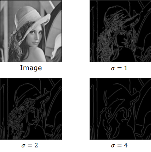
2. Corner Detection (Harris & Moravec Corner Detector)
While edges provide 1D constraints along boundary curves, corners (keypoints / interest points) provide 2D point constraints. A corner is defined as an image location where intensity changes significantly across all 2D spatial directions.
2.1. Why Corners? (2D Constraints & Aperture Problem)
Corners are exceptionally valuable features for camera calibration, 3D reconstruction, optical flow tracking, and object recognition:
- Aperture Problem Mitigation: When viewed through a small local window (aperture), a straight 1D edge suffers from ambiguity along its boundary direction. A corner resolves this ambiguity because its location is constrained in both $x$ and $y$.
- Perceptual Salience: As demonstrated by visual perception experiments (e.g., Ewald Hering’s 1861 orientation illusion), human vision relies heavily on intersecting lines and corner junctions to perceive structural geometry.
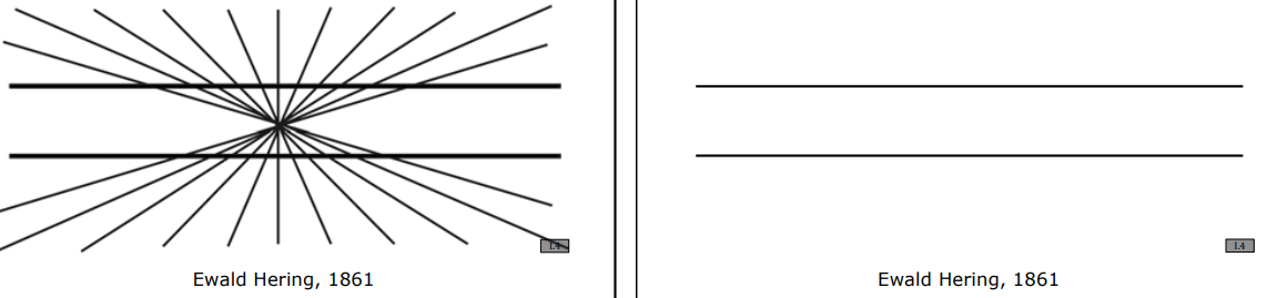
2.2. Categorization of Image Neighborhoods
Local image patches are classified into three fundamental geometric categories based on intensity variation when shifting a local window $W$:
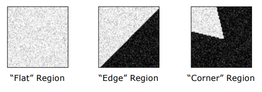
- Flat Region: Shifting the window in any direction results in virtually zero intensity change.
- Edge Region: Shifting the window parallel to the edge direction results in zero intensity change; shifting perpendicular to the edge results in a large intensity change.
- Corner Region: Shifting the window in any spatial direction results in a significant intensity change.
flowchart TD
Patch["Local Image Window W"] --> ShiftTest["Apply Small Spatial Shift (u,v)"]
ShiftTest --> Flat["Flat Region\n(No change in any direction)"]
ShiftTest --> Edge["Edge Region\n(Change in 1 normal direction only)"]
ShiftTest --> Corner["Corner Region\n(Large change in ALL directions)"]
style Patch fill:#1a1a2e,stroke:#16213e,color:#fff
style ShiftTest fill:#16213e,stroke:#4cc9f0,color:#fff
style Flat fill:#16213e,stroke:#888,color:#fff
style Edge fill:#0f3460,stroke:#e94560,color:#fff
style Corner fill:#0f3460,stroke:#4cc9f0,color:#fff
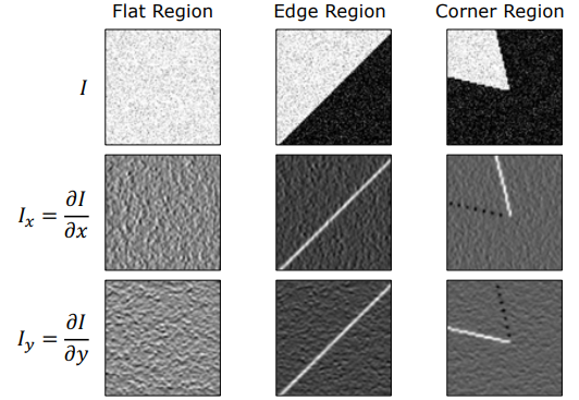
2.3. Mathematical Formulation (Sum of Squared Differences & Taylor Series)
The change in intensity $E(u,v)$ produced by shifting a window $w(x,y)$ by displacement vector $(u,v)$ is formulated using the Sum of Squared Differences (SSD):
$$E(u,v) = \sum_{x,y} w(x,y) \left[ I(x+u, y+v) - I(x,y) \right]^2$$
Where $w(x,y)$ is a window function (either a uniform box window or a 2D Gaussian weighting window $e^{-\frac{x^2+y^2}{2\sigma^2}}$).
Using a first-order 2D Taylor Series expansion for small displacements $(u,v)$:
$$I(x+u, y+v) \approx I(x,y) + u I_x(x,y) + v I_y(x,y)$$
Substituting this back into the SSD equation yields:
$$E(u,v) \approx \sum_{x,y} w(x,y) \left[ u I_x(x,y) + v I_y(x,y) \right]^2$$
Expanding the quadratic term and writing in matrix form:
$$E(u,v) \approx \begin{bmatrix} u & v \end{bmatrix} M \begin{bmatrix} u \[6pt] v \end{bmatrix}$$
Where $M$ is the Second Moment Matrix (also known as the Structure Tensor):
$$M = \sum_{x,y} w(x,y) \begin{bmatrix} I_x^2 & I_x I_y \[6pt] I_x I_y & I_y^2 \end{bmatrix} = \begin{bmatrix} \sum w I_x^2 & \sum w I_x I_y \[6pt] \sum w I_x I_y & \sum w I_y^2 \end{bmatrix}$$
2.4. Second Moment Matrix ($M$) and Eigenvalue Analysis
The Second Moment Matrix $M$ summarizes the local gradient distribution inside the window.
Let $\lambda_1$ and $\lambda_2$ be the two eigenvalues of matrix $M$. These eigenvalues represent the principal curvatures of the local auto-correlation quadratic surface $E(u,v)$:
- $\lambda_1$: Length of the semi-major axis of the gradient uncertainty ellipse.
- $\lambda_2$: Length of the semi-minor axis of the gradient uncertainty ellipse.
Physical Analogy (Moments of Inertia): As established in binary image geometry, the eigenvalues $\lambda_1$ and $\lambda_2$ correspond to the principal moments of inertia of the local gradient scatter mass: $\lambda_1 = E_{max}$ (maximum moment of inertia) and $\lambda_2 = E_{min}$ (minimum moment of inertia).
Classification of Image Regions Based on Eigenvalues:
| Region Type | Eigenvalue Relations | Mathematical Condition | Physical Meaning |
|---|---|---|---|
| Flat Region | $\lambda_1 \approx \lambda_2 \approx 0$ | Both $\lambda_1, \lambda_2$ are small | Insignificant gradient variation in any direction. |
| Edge Region | $\lambda_1 \gg \lambda_2 \approx 0$ | One large $\lambda_1$, one near-zero $\lambda_2$ | Strong gradient variation along 1 normal direction only. |
| Corner Region | $\lambda_1 \approx \lambda_2 \gg 0$ | Both $\lambda_1, \lambda_2$ are large | Strong gradient variation in all spatial directions. |
2.5. Harris Corner Response Function ($R$)
Explicitly calculating eigenvalues $\lambda_1, \lambda_2$ for every single pixel requires taking matrix square roots ($\sqrt{b^2 - 4ac}$), which is computationally expensive. Chris Harris and Mike Stephens (1988) devised an elegant scalar response function $R$ using matrix trace and determinant:
$$\det(M) = \lambda_1 \lambda_2 = (\sum w I_x^2)(\sum w I_y^2) - (\sum w I_x I_y)^2$$
$$\operatorname{trace}(M) = \lambda_1 + \lambda_2 = \sum w I_x^2 + \sum w I_y^2$$
The Harris Corner Response $R$ is defined as:
$$R = \det(M) - k \operatorname{trace}(M)^2 = \lambda_1 \lambda_2 - k (\lambda_1 + \lambda_2)^2$$
Where $k$ is an empirical tunable constant, typically set within $0.04 \le k \le 0.06$.
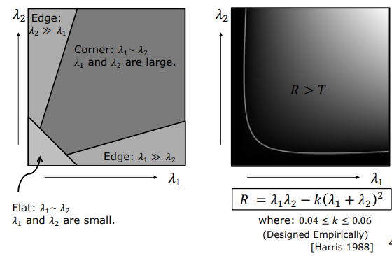
Response Map Partitioning Rules:
- Corner Region: $R > T$ (large positive value).
- Edge Region: $R < -T$ (large negative value, since $\operatorname{trace}(M)^2 \gg \det(M)$).
- Flat Region: $|R| < T$ (small magnitude close to zero).
2.6. Complete Harris Corner Detection Pipeline
The full Harris Corner Detection algorithm proceeds as follows:
flowchart TD
Img["Input Image I(x,y)"] --> Grad["Compute Derivatives Ix and Iy\n(using Sobel kernels)"]
Grad --> Products["Form Derivative Products:\nIx², Iy², IxIy"]
Products --> Gauss["Apply Gaussian Window W_σ:\nSum w*Ix², Sum w*Iy², Sum w*IxIy"]
Gauss --> MatrixM["Construct Structure Tensor M"]
MatrixM --> Resp["Compute Harris Response:\nR = det(M) - k*(trace(M))²"]
Resp --> Thresh["Thresholding: R > Threshold T"]
Thresh --> NMS["Non-Maximum Suppression\n(Find local 3x3 peaks)"]
NMS --> Out["Detected Corner Keypoints"]
style Img fill:#1a1a2e,stroke:#16213e,color:#fff
style Grad fill:#16213e,stroke:#4cc9f0,color:#fff
style Products fill:#16213e,stroke:#4cc9f0,color:#fff
style Gauss fill:#0f3460,stroke:#e94560,color:#fff
style MatrixM fill:#0f3460,stroke:#e94560,color:#fff
style Resp fill:#0f3460,stroke:#e94560,color:#fff
style Thresh fill:#16213e,stroke:#4cc9f0,color:#fff
style NMS fill:#16213e,stroke:#4cc9f0,color:#fff
style Out fill:#1a1a2e,stroke:#4cc9f0,color:#fff
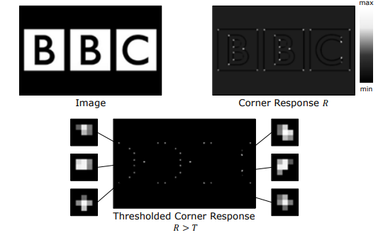
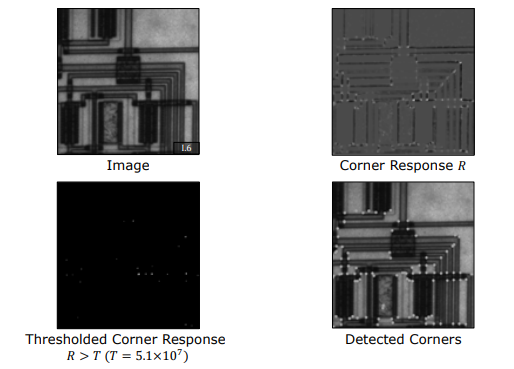
3. Summary Comparison of Edge vs Corner Detection
| Attribute / Property | Canny Edge Detector | Harris Corner Detector |
|---|---|---|
| Constraint Dimension | 1D Spatial Boundary Contours | 2D Point Constraints (Keypoints) |
| Mathematical Basis | Gradient Vector $\nabla I$ + NMS + Hysteresis | Structure Tensor $M$ Eigenvalue Analysis |
| Primary Metric | Gradient Magnitude $ | \nabla I |
| Rotation Invariance | Dependent on gradient quantization | Fully Rotation Invariant (Isotropic Tensor) |
| Scale Sensitivity | Sensitive to Gaussian parameter $\sigma$ | Sensitive to window scale (requires Harris-Laplacian for scale invariance) |
| Primary Applications | Image Segmentation, Object Boundaries | Keypoint Matching, SLAM, Image Stitching, Tracking |
Overview, Fitting Lines and Curves, and Active Contours
- 1. Overview of Boundary Detection
- 2. Fitting Lines and Curves
- 3. Active Contours (Snakes)
This technical note covers Boundary Detection, a fundamental problem in computer vision that bridges the gap between low-level pixel edges and high-level geometric object boundaries. We examine the physical challenges of real-world boundaries, analytical Least Squares Line and Curve Fitting, vertical line failure modes, perpendicular distance normal forms, and dynamic deformable contours known as Active Contours (Snakes) along with their discrete energy optimization.
1. Overview of Boundary Detection
Output from edge detection algorithms consists of discrete, disconnected pixels, noise artifacts, and background clutter. The primary objective of computer vision is to group and fit these pixel fragments into continuous geometric lines or closed curves representing object boundaries (silhouettes). This formulation is known as Boundary Detection.
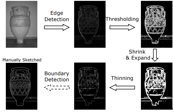
1.1. Key Differences Between Edge Detection and Boundary Detection
- Edge Detection: A local pixel-level operation that detects rapid intensity variations (gradient magnitudes). The output is a binary edge map.
- Boundary Detection: A semantic and geometric global process that aggregates binary edge pixels into structural object contours or parametric curves.
1.2. Principal Physical and Geometric Challenges
Boundary detection algorithms must overcome three major challenges present in natural images:
- Extraneous Data: Images contain thousands of irrelevant edge pixels generated by background textures, surface markings, or illumination shadows. The algorithm must differentiate object boundaries from clutter.
- Incomplete Data and Occlusions: Low contrast, internal object shading, or partial occlusion by other objects cause missing edge fragments and large gaps along object boundaries.
- Image Noise: Sensor noise creates false edge responses in smooth regions and causes true boundary coordinates to shift spatially.
2. Fitting Lines and Curves
The simplest boundary detection task involves fitting a parametric line or low-degree polynomial curve to a set of noisy edge coordinates.
2.1. Preprocessing Pipeline for Edge Images
Raw edge maps are rarely suitable for direct curve fitting. The image undergoes a structured preprocessing sequence:
- Edge Detection & Thresholding: Applying an edge operator (e.g., Sobel) computes gradient magnitudes, which are thresholded to yield a binary edge map.
- Shrink & Expand (Morphology): Morphological shrinking removes isolated noise pixels, after which remaining components are expanded to restore edge continuity.
- Thinning: Thickened edge segments are reduced to single-pixel width, yielding clean coordinate pairs $(x_i, y_i)$ for line/curve fitting.
flowchart LR
A["Input Image"] --> B["Edge Detection & Thresholding"]
B --> C["Shrink & Expand (Morphology)"]
C --> D["Thinning"]
D --> E["Boundary Coordinates (x_i, y_i)"]
style A fill:#1a1a2e,stroke:#e94560,color:#fff
style B fill:#16213e,stroke:#0f3460,color:#fff
style C fill:#16213e,stroke:#0f3460,color:#fff
style D fill:#16213e,stroke:#0f3460,color:#fff
style E fill:#0f3460,stroke:#4cc9f0,color:#fff
2.2. Least Squares Line Fitting
Consider fitting a straight line $y = mx + c$ to a set of $N$ edge points $(x_i, y_i)$ by finding optimal slope $m$ and intercept $c$.
2.2.1. Vertical Distance Minimization
The standard formulation minimizes the average squared vertical distance from each point to the candidate line.
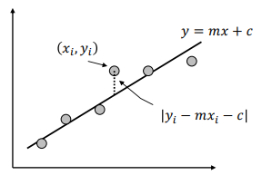
The vertical distance from point $(x_i, y_i)$ to the line is $y_i - mx_i - c$. The mean squared error energy (cost) function is defined as:
$$E = \frac{1}{N} \sum_{i=1}^{N} (y_i - m x_i - c)^2$$
Setting the partial derivatives with respect to $m$ and $c$ to zero yields:
$$\frac{\partial E}{\partial m} = 0 \implies \sum_{i=1}^{N} (y_i - m x_i - c)x_i = 0$$
$$\frac{\partial E}{\partial c} = 0 \implies \sum_{i=1}^{N} (y_i - m x_i - c) = 0$$
Solving for intercept $c$ from the second equation:
$$c = \bar{y} - m\bar{x} \quad \text{where} \quad \bar{x} = \frac{1}{N}\sum_{i=1}^N x_i, \quad \bar{y} = \frac{1}{N}\sum_{i=1}^N y_i$$
Substituting $c$ into the first equation yields the closed-form analytical solution for slope $m$:
$$m = \frac{\sum_{i=1}^{N} (x_i - \bar{x})(y_i - \bar{y})}{\sum_{i=1}^{N} (x_i - \bar{x})^2}$$
2.2.2. The Vertical Line Failure Mode
Vertical distance minimization fails completely when edge points form a near-vertical line.
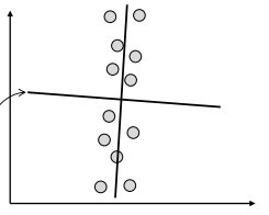
- Physical Cause: The slope of a vertical line approaches infinity ($m \to \infty$). The denominator term $\sum (x_i - \bar{x})^2$ approaches zero, causing numerical breakdown.
- Pathological Behavior: Because the cost function measures vertical distances, vertical offsets to a true vertical line are infinite. To minimize these vertical offsets, the algorithm rotates the candidate line to horizontal—producing an entirely incorrect fit.
2.3. Perpendicular Distance Minimization
To eliminate vertical singularities, lines are expressed using the normal parameterization:
$$x \sin\theta - y \cos\theta + \rho = 0$$
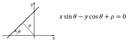
Here, $\theta$ represents the angle of the normal vector with the x-axis, and $\rho$ is the perpendicular distance from the origin to the line. The perpendicular distance $r_i$ from point $(x_i, y_i)$ to the line is:
$$r_i = x_i \sin\theta - y_i \cos\theta + \rho$$
The objective energy function minimizes mean squared perpendicular distances:
$$E = \frac{1}{N} \sum_{i=1}^{N} (x_i \sin\theta - y_i \cos\theta + \rho)^2$$
Key Insight (Equivalence to Axis of Minimum Second Moment): Perpendicular distance minimization is mathematically identical to finding the axis of minimum second moment in binary image analysis.
Treating point coordinates as binary image pixels, the central second moments relative to the centroid $(\bar{x}, \bar{y})$ are:
$$a = \sum_{i=1}^N (x_i - \bar{x})^2, \quad c = \sum_{i=1}^N (y_i - \bar{y})^2, \quad b = 2 \sum_{i=1}^N (x_i - \bar{x})(y_i - \bar{y})$$
Solving for parameters $\theta$ and $\rho$ provides a numerically stable fit for all orientations, including vertical lines:
$$\tan(2\theta) = \frac{b}{a - c}$$
$$\rho = \bar{y}\cos\theta - \bar{x}\sin\theta$$
2.4. Curve Fitting and Overdetermined Linear Systems
When boundaries exhibit curvature, higher-order polynomial models such as cubic polynomials ($y = ax^3 + bx^2 + cx + d$) are employed.
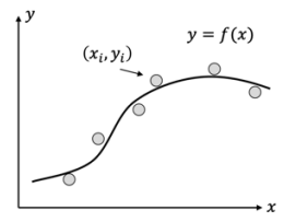
The vertical squared error energy is:
$$E = \frac{1}{N} \sum_{i=1}^{N} (y_i - a x_i^3 - b x_i^2 - c x_i - d)^2$$
Rather than solving complex system derivatives manually, the problem is formulated as an overdetermined linear system of equations.
Evaluating each coordinate pair $(x_i, y_i)$ yields $N$ linear equations:
$$\begin{aligned} y_1 &= a x_1^3 + b x_1^2 + c x_1 + d \ y_2 &= a x_2^3 + b x_2^2 + c x_2 + d \ &\ \ \vdots \ y_N &= a x_N^3 + b x_N^2 + c x_N + d \end{aligned}$$
With $m$ unknown coefficients (here $m=4$: $a, b, c, d$) and $N$ data points ($N > m$), the system is written in matrix form:
$$X a = y$$
$$\begin{bmatrix} x_1^3 & x_1^2 & x_1 & 1 \ x_2^3 & x_2^2 & x_2 & 1 \ \vdots & \vdots & \vdots & \vdots \ x_N^3 & x_N^2 & x_N & 1 \end{bmatrix}{N \times m} \begin{bmatrix} a \ b \ c \ d \end{bmatrix}{m \times 1} = \begin{bmatrix} y_1 \ y_2 \ \vdots \ y_N \end{bmatrix}_{N \times 1}$$
Since input matrix $X$ ($N \times m$) is non-square, its direct matrix inverse does not exist. Premultiplying both sides by $X^T$ converts the system into an $m \times m$ square matrix:
$$X^T X a = X^T y \implies a = (X^T X)^{-1} X^T y$$
The matrix $X^+ = (X^T X)^{-1} X^T$ is the Moore-Penrose Pseudo-Inverse. This linear algebraic solution provides a robust closed-form fit for polynomial curve fitting of any degree.
3. Active Contours (Snakes)
Active Contours (Snakes) are dynamic, deformable energy-minimizing curves placed in the vicinity of an object boundary. Under internal structural forces and external image forces, the contour iteratively contracts and shapes itself until it locks onto salient image boundaries like an elastic band.
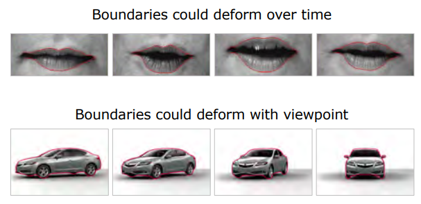
3.1. Discrete Representation of Contours
A contour is discretized into an ordered sequence of $N$ control points (vertices) connected by straight segments of uniform length:
$$v_i = (x_i, y_i) \quad \text{for} \quad i = 0, 1, 2, \dots, N-1$$
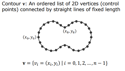

3.2. Energy Formulation and Force Balance
Contour deformation is governed by balancing internal forces (maintaining curve smoothness) against external forces (attracting the curve to image boundaries).
3.2.1. Internal Contour Energy ($E_{contour}$)
Internal bending energy prevents the contour from developing severe kinks, tangles, or oscillations under noisy conditions. It combines two physical properties:
- Elasticity ($E_{elastic}$): Encourages contraction like a rubber band, keeping distances between neighboring vertices minimal. In continuous form it corresponds to the squared first derivative ($|\frac{\partial v}{\partial s}|^2$), discretized as squared differences between adjacent vertices:
$$E_{elastic} = \sum_{i=0}^{N-1} |v_{i+1} - v_i|^2$$
- Smoothness ($E_{smooth}$): Minimizes curvature, preventing sharp corners and making the curve bend smoothly like a thin metal strip. In continuous form it corresponds to the squared second derivative ($|\frac{\partial^2 v}{\partial s^2}|^2$), discretized via second-order differences:
$$E_{smooth} = \sum_{i=0}^{N-1} |v_{i+1} - 2v_i + v_{i-1}|^2$$
Combining both components with weighting parameters $\alpha$ and $\beta$ yields the internal contour energy:
$$E_{contour} = \alpha E_{elastic} + \beta E_{smooth} = \alpha \sum_{i=0}^{N-1} |v_{i+1} - v_i|^2 + \beta \sum_{i=0}^{N-1} |v_{i+1} - 2v_i + v_{i-1}|^2$$
3.2.2. External Image Energy ($E_{image}$)
External forces pull the contour toward high-gradient image edges using squared gradient magnitude ($|\nabla I|^2$). However, if the contour is distant from boundaries, edge gradients drop to zero, leaving no attraction force.
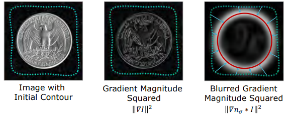
The Gaussian Blurring Trick: Convolving the gradient map with a broad Gaussian filter ($G_\sigma$) spreads out edge forces into a wide potential field. This attraction field enables distant control points to feel pulling forces toward object boundaries.
Because energy minimization drives the snake into potential wells, external energy is negated:
$$E_{image} = - \sum_{i=0}^{N-1} |\nabla (G_\sigma * I(v_i))|^2$$
3.2.3. Total Energy ($E_{total}$)
The total energy optimized by the active contour model is the sum of internal and external energies:
$$E_{total} = E_{image} + E_{contour}$$
3.3. Contour Deformation via the Greedy Algorithm
Minimizing total energy is commonly implemented using a fast, practical Greedy Algorithm:
- Uniform Re-sampling: Vertices are redistributed along the curve to maintain equal spacing between adjacent control points.
- Critical Importance: Without uniform re-sampling, elastic forces cause control points to bunch together, tangling the curve geometry.
- Local Neighborhood Search: For each vertex $v_i$, candidates within a small neighborhood window $W$ (e.g., $3 \times 3$ or $5 \times 5$ pixels) are evaluated. The vertex moves to the neighbor that minimizes local $E_{total}$.
- Termination Condition: Iteration stops when total vertex displacement across the contour drops below a small threshold $\epsilon$. Otherwise, the process repeats from Step 1.

3.4. Parameter Analysis and Advanced Extensions
3.4.1. Impact of Elasticity Parameter $\alpha$
The elasticity coefficient $\alpha$ controls how strongly the snake contracts.
- Large $\alpha$: High elastic tension pulls the curve tightly into narrow concave gaps between adjacent objects.
- Small $\alpha$: Low elastic tension keeps the curve relaxed, bridging over narrow gaps without snapping inwards.
3.4.2. Model Limitations and Advanced Formulations
- Initialization Sensitivity: Active contours require reasonable initial guesses. If initialized far outside the attraction zone, the snake fails to lock onto the target and gets trapped in local background clutter.
- Ballooning Forces: While standard snakes contract inward, adding an outward pressure (balloon) force expands the contour from inside an object out to its boundaries.
- Prior Shape Models: For objects with known shape geometry (e.g., hearts, eyes, or hands), a prior shape energy term $E_{prior}$ penalizes deviations from expected structural templates.
Hough Transform and Generalized Hough Transform
This technical note covers Hough Transform and Generalized Hough Transform (GHT), powerful voting mechanisms in computer vision used to detect parametric primitives (lines, circles) and arbitrary non-parametric shapes in noisy binary edge maps with missing fragments and clutter.
1. Hough Transform
Binary edge maps produced by low-level edge detectors contain background clutter, disconnected fragments, and noise. Classical line fitting methods can fail completely when outliers are present.
The Hough Transform overcomes the inlier-outlier problem by converting pixel detection in image space into a robust voting procedure in a discrete parameter space.
1.1. Line Detection
Consider detecting straight lines in an image using the Cartesian line equation $y = mx + c$.
1.1.1. Geometrical Duality Concept
Rewriting the line equation in terms of parameters yields:
$$c = - m x_i + y_i$$
This relationship establishes a fundamental geometric duality between Image Space ($x-y$) and Parameter Space ($m-c$):
- A Single Point $(x_i, y_i)$ in Image Space: Maps to a straight line $c = -x_i m + y_i$ in parameter space. This line represents all possible $(m, c)$ combinations passing through $(x_i, y_i)$.
- A Straight Line in Image Space: Maps to a single point $(m^, c^)$ in parameter space.
- Intersection Logic: Collinear pixels lying on the same line in image space correspond to intersecting lines in parameter space that concur at a single point $(m^, c^)$. Outlier noise pixels map to independent non-concurring lines.
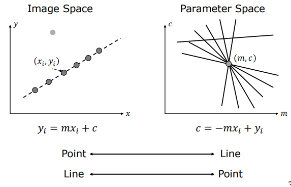
flowchart LR
subgraph ImageSpace ["Image Space (x-y)"]
P1["Point (x1, y1)"]
P2["Point (x2, y2)"]
Line1["Common Line y = m* x + c*"]
end
subgraph ParamSpace ["Parameter Space (m-c)"]
L1["Line c = -x1 m + y1"]
L2["Line c = -x2 m + y2"]
Intersect["Intersection Point (m*, c*)"]
end
P1 --> L1
P2 --> L2
L1 --> Intersect
L2 --> Intersect
Line1 <--> Intersect
style ImageSpace fill:#1a1a2e,stroke:#e94560,color:#fff
style ParamSpace fill:#16213e,stroke:#4cc9f0,color:#fff
1.1.2. Polar Normal Parametrization ($\theta - \rho$)
The slope-intercept parameterization $y = mx + c$ fails for vertical lines because $m \to \infty$, requiring an unbounded parameter space. To resolve this, the polar normal parametrization is used:
$$x \sin\theta - y \cos\theta + \rho = 0 \implies \rho = y_i \cos\theta - x_i \sin\theta$$
Where:
- $\theta \in [0, \pi)$: The bounded angle of the line’s normal vector with the x-axis.
- $\rho \in [-\sqrt{M^2+N^2}, \sqrt{M^2+N^2}]$: The perpendicular distance from the origin to the line (bounded by the image diagonal).
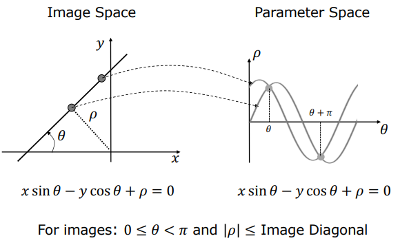
1.1.3. The Accumulator Voting Algorithm
Line detection via Hough voting executes the following algorithmic steps:
- Parameter Space Discretization: The $(\theta, \rho)$ domain is quantized into a 2D discrete accumulator array $A(\theta, \rho)$, initialized to zero.
- Voting Procedure: For each edge pixel $(x_i, y_i)$, $\theta$ is stepped from $0$ to $\pi$, computing $\rho = y_i \cos\theta - x_i \sin\theta$. The corresponding accumulator bin is incremented:
$$A(\theta, \rho) = A(\theta, \rho) + 1$$
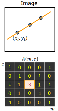
- Peak Finding: After voting completes, local maxima (peaks) in $A(\theta, \rho)$ are extracted. Peak bin coordinates correspond directly to line parameters $(\theta^, \rho^)$ in image space.
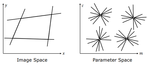
1.1.4. Practical Engineering Trade-offs
- Bin Resolution Selection: Coarse quantization (low resolution) merges distinct lines into single accumulator bins, reducing angular precision. Fine quantization (high resolution) splits votes across neighboring bins due to noise and discretization errors, obscuring peaks.
- Patch Voting: To improve noise robustness, each edge point casts votes into a small Gaussian-weighted patch of accumulator bins rather than a single discrete bin.
- Peak Extraction & NMS: Noise causes vote clusters around true peak values. A Non-Maximal Suppression (NMS) algorithm isolates distinct local peaks and filters out spurious detections.
1.2. Circle Detection
The geometric equation of a circle involves three parameters:
$$(x - a)^2 + (y - b)^2 = r^2$$
Where $(a, b)$ are center coordinates and $r$ is the radius.
1.2.1. Known Radius $r$ (2D Parameter Space $A(a, b)$)
If the radius $r$ is fixed, the parameter space is 2D: $A(a, b)$. Each edge point $(x_i, y_i)$ votes along a circle of radius $r$ centered at $(x_i, y_i)$ in parameter space.
The intersection of these voting circles pinpoints the true circle center $(a^, b^)$.
1.2.2. Fast Voting Using Edge Orientation (Gradient Direction)
When edge gradient orientation $\phi_i$ is known, the circle center must lie along the normal direction at distance $r$ from edge point $(x_i, y_i)$.
Instead of voting along an entire circle, votes are cast into only two candidate center locations:
$$a = x_i \pm r \cos\phi_i \quad \text{and} \quad b = y_i \pm r \sin\phi_i$$
Key Insight: Incorporating gradient directions reduces voting complexity from $\mathcal{O}(N \cdot 360)$ to $\mathcal{O}(N \cdot 2)$, achieving massive speedups and dramatically reducing noise accumulation.
1.2.3. Unknown Radius $r$ (3D Parameter Space $A(a, b, r)$)
When radius $r$ is unknown, the parameter space expands to 3D: $A(a, b, r)$. Each edge point casts votes along a 3D cone surface. As parameters increase beyond three, accumulator memory and computation scale exponentially, making classical Hough voting intractable.
2. Generalized Hough Transform (GHT)
While the classical Hough transform detects shapes defined by analytic equations (lines, circles, ellipses), the Generalized Hough Transform (GHT) detects arbitrary non-parametric shapes (e.g., logos, animals, or vehicle outlines) using a template-driven voting table.
2.1. Offline Model Construction and the $\phi$-Table
Before searching an image, a geometric model of the target template shape is extracted offline:
- Reference Point Selection: An arbitrary reference point $(x_c, y_c)$ (e.g., centroid) is chosen inside the template boundary.
- Boundary Vector Extraction: For each boundary point $v_i$, the local edge orientation angle $\phi_i$ is computed.
- Polar Vector Computation: A displacement vector $r = (r_i, \alpha_i)$ from $(x_c, y_c)$ to boundary point $v_i$ is calculated:
- $r_i = \sqrt{(x_i - x_c)^2 + (y_i - y_c)^2}$: Distance to reference center.
- $\alpha_i = \operatorname{atan2}(y_c - y_i, x_c - x_i)$: Direction angle of displacement vector.
- $\phi$-Table Construction: Indexed by edge orientation angle $\phi$, the table stores lists of displacement vectors $(r, \alpha)$ associated with each orientation angle.
2.2. Online Detection Procedure
Searching for the target template in an unseen image proceeds as follows:
- Initialize a 2D accumulator array $A(x_c, y_c)$ to zero.
- For each edge pixel $(x_i, y_i)$ with gradient orientation $\phi_i$:
- Look up matching displacement vectors $(r, \alpha)$ in the $\phi$-Table using index $\phi_i$.
- Calculate candidate reference center coordinates for each vector:
$$x_c = x_i + r \cos\alpha \quad \text{and} \quad y_c = y_i + r \sin\alpha$$
- Increment the accumulator bin:
$$A(x_c, y_c) = A(x_c, y_c) + 1$$
- Locate local maxima (peaks) in $A(x_c, y_c)$. Peak coordinates correspond to detected target reference centers $(x_c, y_c)$ in the search image.
2.3. Handling Scale and Rotation Variances
If the target object appears under unknown uniform scaling $s$ and rotation angle $\theta$, the parameter space expands to a 4D accumulator $A(x_c, y_c, s, \theta)$.
The reference center equation is updated:
$$x_c = x_i + r \cdot s \cdot \cos(\alpha + \theta)$$
$$y_c = y_i + r \cdot s \cdot \sin(\alpha + \theta)$$
Algorithmic Limitation: Voting in 4D space requires excessive memory and computational complexity ($\mathcal{O}(N \cdot S \cdot R)$), making 4D GHT impractically slow for real-time applications without hierarchical optimization.
SIFT Detector and Descriptor
- 1. Overview
- 2. What is an Interest Point?
- 3. Detecting Blobs
- 4. SIFT Detector
- 5. SIFT Descriptor
- 6. Technical Summary Matrix
1. Overview
In traditional computer vision approaches, binary segmentation and geometric moment analysis are quite effective for object recognition and localization. However, these methods only demonstrate stability in strictly controlled industrial environments (backlit silhouettes) or high-contrast text extraction applications (license plate recognition, etc.).
When it comes to recognizing three-dimensional or complex planar two-dimensional objects in real-world scenes, these simplistic approaches fail completely.
Limitations of Traditional Template Matching:
─────────────────────────────────────────────
1. Scale Changes: Variations in object size due to depth.
2. Rotation: 2D in-plane and 3D out-of-plane rotations.
3. Occlusion: Partial blockage of the object of interest.
4. Illumination: Variations in lighting, specularities, and camera gain.
If one attempts to use classic template matching or normalized cross-correlation (NCC) to find an object, thousands of partial sub-templates must be generated for all possible rotation angles and scale factors, and slid across the entire image. This process reaches a computational complexity of $O(N \cdot M \cdot S \cdot R)$, making it completely intractable for practical systems.
Key Insight: Overcoming this fundamental problem relies on extracting highly descriptive and unique local features directly from the image that are invariant to geometric and photometric transformations. Once their spatial coordinates and local appearance signatures (descriptors) are extracted, keypoints across different images can be matched one-to-one for object recognition, image stitching, and 3D reconstruction.
2. What is an Interest Point?
An interest point in an image is a local region that possesses the richest visual information and uniqueness. For a local patch to qualify as an interest point, it must fulfill several critical criteria:
Desirable Properties of an Ideal Interest Point:
- Rich Content: The local analysis window must contain high variance in intensity/color.
- Well-defined Representation: A compact, distinctive visual signature (descriptor) must be computable from the local texture around the point for matching.
- Well-defined Position: The interest point must have a precise spatial coordinate ($x, y$) in the image plane for spatial accuracy.
- Scale and Rotation Invariance: Even when the object scales up/down or rotates, the same spatial location and signature must be reliably detected (repeatability).
- Insensitivity to Illumination: It must remain stable under shadows, specular highlights, and camera gain adjustments.
Evaluating Lines, Edges, Corners, and Blobs:
- Edges: Edges are regions where intensity changes rapidly in a single direction. Sliding a local window along an edge line reveals virtually no appearance change (aperture problem). This spatial ambiguity makes edges unsuitable as interest points.
- Corners: Corners represent the intersection of two distinct edge directions, providing well-defined spatial localization ($x, y$). However, they lack sufficiently rich local appearance information to represent complex textured objects and occur sparsely.
- Blobs and Patches: Circular or elliptical patches characterized by a specific spatial scale ($\sigma$), a dominant orientation ($\theta$), and rich internal texture variation. Because their location, scale, and local texture can be mathematically modeled with high stability, Blob structures represent the ideal interest point candidate in computer vision.
3. Detecting Blobs
Mathematically, detecting a blob corresponds to finding local intensity extrema (peaks) across different spatial resolution levels (scale-space).
3.1 1D Signal Second Derivatives and Scale-Space
In a 1D signal, noise is smoothed using a Gaussian filter of standard deviation $\sigma$:
$$G(x, \sigma) = \frac{1}{\sqrt{2\pi}\sigma} e^{-\frac{x^2}{2\sigma^2}}$$
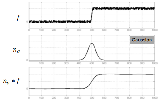
Convolving the signal with the first derivative of a Gaussian ($\frac{d}{dx} G_\sigma$) produces a peak response at step transitions.
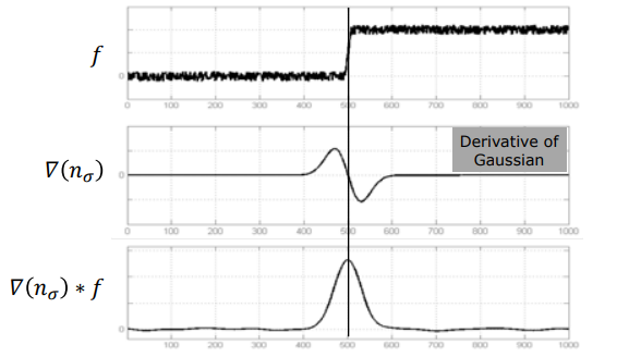
Applying the second derivative of a Gaussian ($\frac{d^2}{dx^2} G_\sigma$ / Inverted Mexican Hat) yields a Zero-Crossing at the exact center of the edge.
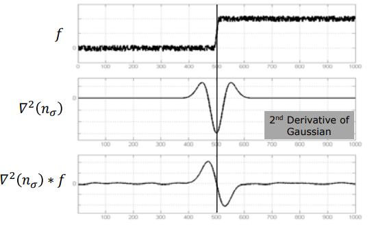
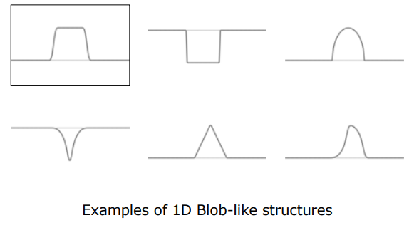
To analyze blobs of varying widths (e.g., Blobs $A, B, C$ with widths $W, 2W, 3W$), a Scale-Space is constructed by continuously increasing the filter standard deviation ($\sigma$):
$$S(x, \sigma) = f(x) * G(x, \sigma)$$
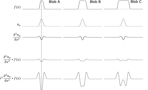
3.2 $\sigma^2$-Normalization and Characteristic Scale
As the Gaussian standard deviation ($\sigma$) increases (coarser scale), the peak amplitude of the filter decreases, dampening the response. To compare extrema across different scale levels consistently, the second derivative filter is multiplied by a scaling factor of $\sigma^2$. This yields the $\sigma$-normalized derivative response:
$$\text{NLoG}{1D} = \sigma^2 \frac{d^2 G\sigma}{dx^2} * f(x)$$
Plotting the normalized response amplitude at a blob’s center across values of $\sigma$ reveals a maximum (local extremum) at a scale proportional to the blob’s spatial size ($\sigma^* \propto \text{Blob Width}$):
- Blob $A$ ($\text{Width}=W$): Peak response at $\sigma_A^* = \sigma_1$.
- Blob $B$ ($\text{Width}=2W$): Peak response at $\sigma_B^* = 2\sigma_1$.
- Blob $C$ ($\text{Width}=3W$): Peak response at $\sigma_C^* = 3\sigma_1$.
Characteristic Scale: The unique scale $\sigma^$ where the normalized operator reaches a local maximum is called the Characteristic Scale. Searching for extrema in 2D $(x, \sigma)$-space simultaneously yields both the exact spatial location ($x^$) and the true physical scale ($\sigma^*$) of the blob.
3.3 2D Normalized Laplacian of Gaussian (NLoG)
In 2D images, the equivalent of the 1D normalized second derivative is the Normalized Laplacian of Gaussian (NLoG) operator. It is formed by taking the Laplacian ($\nabla^2 = \frac{\partial^2}{\partial x^2} + \frac{\partial^2}{\partial y^2}$) of a 2D Gaussian and scaling by $\sigma^2$:
$$\text{NLoG}_{2D} = \sigma^2 \nabla^2 G(x, y, \sigma) = \sigma^2 \left( \frac{\partial^2 G}{\partial x^2} + \frac{\partial^2 G}{\partial y^2} \right)$$
$$\text{NLoG}_{2D}(x, y, \sigma) = -\frac{1}{2\pi\sigma^2} \left( 2 - \frac{x^2 + y^2}{\sigma^2} \right) e^{-\frac{x^2+y^2}{2\sigma^2}}$$
Convolving an image with NLoG filters across multiple scale levels produces a 3D Scale-Space Volume:
$$V(x, y, \sigma) = I(x, y) * \left[ \sigma^2 \nabla^2 G(x, y, \sigma) \right]$$
Local extrema points $(x^, y^, \sigma^*)$ extracted within this 3D volume represent the true locations and scales of all image blobs.
4. SIFT Detector
Developed by David Lowe, the SIFT (Scale-Invariant Feature Transform) detector introduces key engineering innovations to make scale-space blob detection computationally efficient, fast, and robust to noise.
4.1 Fast NLoG Approximation: Difference of Gaussians (DoG)
Computing 2D NLoG convolutions at every scale level is computationally expensive. Lowe demonstrated that subtracting two adjacent Gaussian-smoothed images in scale-space—known as the Difference of Gaussians (DoG) operator—provides a close mathematical approximation to NLoG:
$$\text{DoG}(x, y, \sigma) = S(x, y, k\sigma) - S(x, y, \sigma) = I(x, y) * \left[ G(x, y, k\sigma) - G(x, y, \sigma) \right]$$
From the heat diffusion equation, the limit relationship yields:
$$\frac{\partial G}{\partial \sigma} = \lim_{\Delta\sigma \to 0} \frac{G(x,y,\sigma + \Delta\sigma) - G(x,y,\sigma)}{\Delta\sigma}$$
$$\sigma \nabla^2 G = \frac{\partial G}{\partial \sigma} \approx \frac{G(x,y,k\sigma) - G(x,y,\sigma)}{(k-1)\sigma}$$
Multiplying both sides by $\sigma$ directly relates DoG to the $\sigma$-normalized NLoG:
$$G(x,y,k\sigma) - G(x,y,\sigma) \approx (k-1) \cdot \left[ \sigma^2 \nabla^2 G \right] = (k-1) \cdot \text{NLoG}$$
By simply taking pixel-wise differences between adjacent Gaussian-blurred images, the expensive NLoG calculation is replaced by efficient image subtraction.
4.2 3D Extremum Search and Filtering Weak Keypoints
To detect stable keypoints in the DoG volume:
- A $3 \times 3 \times 3$ cubic window is centered over each sample point in the DoG stack.
- The pixel’s value is compared against its 8 spatial neighbors at the current scale, 9 neighbors at the scale above, and 9 neighbors at the scale below (a total of 26 neighbors).
- If the central pixel is strictly greater than or less than all 26 neighbors, it is designated as a keypoint candidate.
Pruning Low-Contrast and Edge Responses: Candidate keypoints with low contrast are discarded by thresholding DoG value magnitude. Additionally, unstable keypoints along edges are eliminated by checking the eigenvalue ratio of the local 2D Hessian matrix. The remaining points form the finalized set of stable SIFT interest points.
4.3 Achieving Scale and Rotation Invariance
1. Scale Invariance
Changes in camera distance alter object magnification, causing DoG peak extrema to shift to different Characteristic Scales ($\sigma^$). The ratio of these scales ($\frac{\sigma_1^}{\sigma_2^*}$) reflects the physical magnification ratio. SIFT normalizes keypoint regions by resampling local patches according to their characteristic scale radius before descriptor extraction.
2. Rotation Invariance and Principal Orientation
A square patch window is constructed around each keypoint at its characteristic scale.
- For every pixel in the window, horizontal ($I_x$) and vertical ($I_y$) partial derivatives are computed to yield gradient magnitude ($m$) and orientation ($\theta$):
$$m(x,y) = \sqrt{I_x^2 + I_y^2} \quad \text{and} \quad \theta(x,y) = \tan^{-1}\left( \frac{I_y}{I_x} \right)$$
- To gain immunity against lighting changes, gradient magnitudes are discarded and only orientation angles ($\theta$) are accumulated.
- Orientation angles ($0^\circ - 360^\circ$) are binned into a 36-bin Gradient Orientation Histogram.
- The dominant peak in the histogram defines the keypoint’s Principal Orientation ($\theta_{\text{principal}}$).
- During matching, the patch is rotated backward by $\theta_{\text{principal}}$, aligning it upright (North). This eliminates in-plane rotation effects.
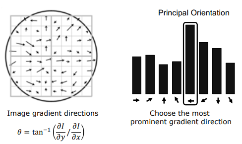
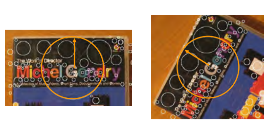
5. SIFT Descriptor
Once scale and orientation effects are normalized, a compact and distinctive local descriptor vector must be generated from the upright patch.
5.1 Mathematical Construction of the SIFT Descriptor
- A pixel grid is established over the normalized, oriented keypoint patch.
- Only gradient orientation angles ($\theta$) are evaluated to maintain illumination insensitivity.
- The patch area is divided into 4 non-overlapping spatial quadrants ($2 \times 2$).
- An 8-bin local orientation histogram ($0^\circ, 45^\circ, 90^\circ, \dots, 315^\circ$) is computed independently for each quadrant.
- The 4 quadrant histograms are concatenated into a unified vector.
- In Lowe’s standard implementation, a $16 \times 16$ pixel region is partitioned into a $4 \times 4$ array of sub-regions, generating an 8-bin histogram per sub-region. This yields the famous 128-dimensional SIFT Descriptor vector ($16 \times 8 = 128$).
Grid Structure 4 Quadrant Histograms
┌──────────┬──────────┐
│ │ │ Local Hist 1 ──┐
│ Quadrant │ Quadrant │ Local Hist 2 ──┼──► Concatenate ──► [ SIFT Descriptor Vector ]
│ 1 │ 2 │ Local Hist 3 ──┼──► (128D Invariant Signature)
├──────────┼──────────┤ Local Hist 4 ──┘
│ Quadrant │ Quadrant │
│ 3 │ 4 │
└──────────┴──────────┘
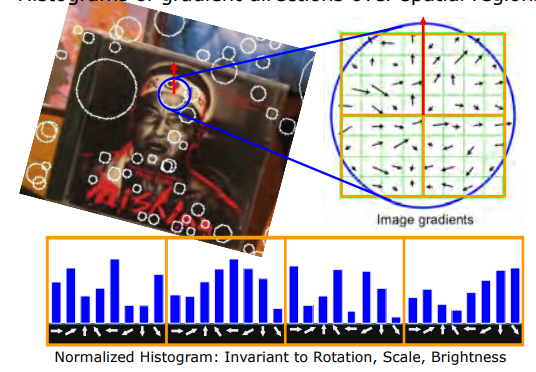
5.2 Distance Metrics for Matching SIFT Descriptors ($H_1, H_2$)
-
L2 Distance (Euclidean Distance): Square root of the sum of squared differences between descriptor entries. Values closer to zero indicate strong similarity:
$$D(H_1, H_2) = \sqrt{\sum_{k} \left( H_1[k] - H_2[k] \right)^2}$$
-
Normalized Correlation: Mean-centered descriptor correlation scaled by total energy. A value of 1.0 indicates perfect linear agreement:
$$D(H_1, H_2) = \frac{\sum_{k} (H_1[k] - \mu_1)(H_2[k] - \mu_2)}{\sqrt{\sum_{k} (H_1[k] - \mu_1)^2 \sum_{k} (H_2[k] - \mu_2)^2}} \quad \text{where} \quad \mu = \frac{1}{N} \sum_{k} H[k]$$
-
Intersection Metric: Sum of minimum values across corresponding histogram bins, representing overlap area:
$$D(H_1, H_2) = \sum_{k} \min\left( H_1[k], H_2[k] \right)$$
5.3 SIFT Matching Examples and Applications
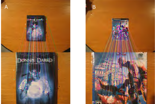
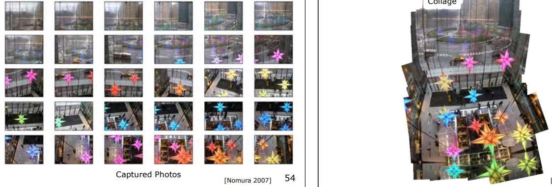
5.4 Limitations of SIFT and 3D Viewpoint Sensitivity
While SIFT produces hundreds of stable matches for 2D planar surfaces undergoing rotation, scaling, and occlusion, SIFT breaks down when applied to 3D non-planar objects.
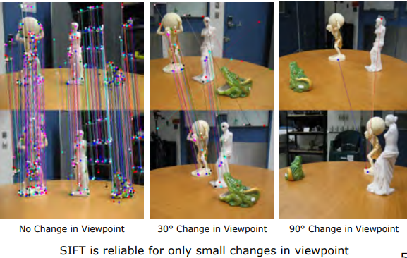
As camera viewpoint changes relative to a 3D object, out-of-plane rotations alter local appearance due to 3D self-occlusion and perspective deformation. Empirical studies demonstrate:
- At a $30^\circ$ viewpoint shift: The number of matched SIFT keypoints drops drastically.
- At a $90^\circ$ viewpoint shift: Keypoint correspondences degrade completely, yielding zero valid matches.
Conclusion: SIFT is reliable primarily for 2D planar scenes or small 3D viewpoint variations.
6. Technical Summary Matrix
| Module / Topic | Core Equation | Target Output / Value | Problem Solved | Fundamental Limitation |
|---|---|---|---|---|
| Interest Point | Circular patch (Blobs) | Spatial location ($x, y$), scale radius ($\sigma$), and orientation ($\theta$). | Resolves sliding edge ambiguity (aperture problem) and corner sparsity. | Homogeneous, flat, untextured image regions. |
| Blob Detection | $\text{NLoG} = \sigma^2 \nabla^2 G$ | Characteristic Scale ($\sigma^$) and location ($x^, y^*$). | Detects objects across scale via 3D scale-space extrema search. | High computational cost of multi-scale 2D Gaussian convolutions. |
| SIFT Detector | $\text{DoG} = S(k\sigma) - S(\sigma)$ | Scale and rotation normalized keypoints. | Fast NLoG approximation via DoG and principal orientation assignment. | Noisy and unstable extrema candidates across adjacent scales. |
| SIFT Descriptor | Vector Concatenation | 128-dimensional invariant visual signature. | Enables stable matching under occlusion, rotation, and illumination. | Total breakdown on 3D objects with $30^\circ - 90^\circ$ viewpoint shifts. |
Overview and Image Transformations
- 1. Classification of Image Transformations
- 2. 2x2 Linear Transformations
- 3. 3x3 Image Transformations
- 4. Transformation Properties Summary
1. Classification of Image Transformations
Transformations applied in computer vision and image processing fall into two main categories:
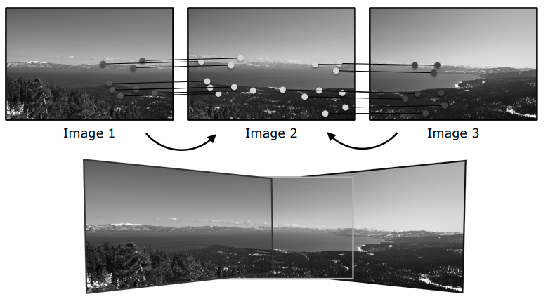
1.1 Image Filtering (Range Transformations)
In image filtering, the pixel spatial coordinates (domain) of the input image remain strictly fixed, while pixel intensity and color values (range) are modified. Pixel processing, linear filtering, and convolution belong to this class. The geometric structure and boundaries of the image remain completely unchanged.
Mathematical formulation:
$$g(x,y) = T_r(f(x,y))$$
where $f(x,y)$ represents the input image, $g(x,y)$ the output image, and $T_r$ the intensity/range transformation operator.
1.2 Image Warping (Domain Transformations)
In image warping, operations work directly on the spatial coordinate plane (domain) of the image, altering its geometric shape. Translation, rotation, scaling, affine, and projective transformations belong to this class.
Mathematical formulation:
$$g(x,y) = f(T_d(x,y))$$
where $T_d$ represents the spatial coordinate transformation operator.
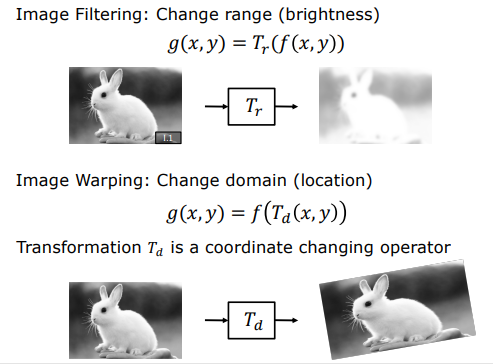
[Image Filtering (Range)] [Image Warping (Domain)]
f(x, y) ──► T_r ──► g(x, y) f(x, y) ──► T_d(x, y) ──► g(x', y')
(Pixel values change, (Pixel locations change,
coordinates fixed) shape warped)
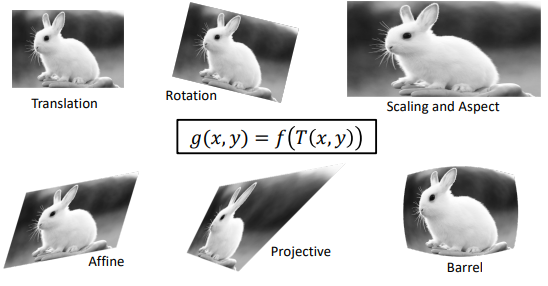
2. 2x2 Linear Transformations
The most fundamental geometric operations in two-dimensional space map input pixels to output pixels via a $2 \times 2$ matrix $T$. Given a source pixel $p_1(x_1, y_1)$ and target pixel $p_2(x_2, y_2)$:
$$\begin{bmatrix} x_2 \ y_2 \end{bmatrix} = \begin{bmatrix} t_{11} & t_{12} \ t_{21} & t_{22} \end{bmatrix} \begin{bmatrix} x_1 \ y_1 \end{bmatrix}$$
2.1 Scaling (Stretching & Squishing)
To stretch or shrink an image horizontally by factor $a$ and vertically by factor $b$, the coordinate equations are:
$$x_2 = a \cdot x_1, \quad y_2 = b \cdot y_1$$
In matrix form:
$$\begin{bmatrix} x_2 \ y_2 \end{bmatrix} = \begin{bmatrix} a & 0 \ 0 & b \end{bmatrix} \begin{bmatrix} x_1 \ y_1 \end{bmatrix}$$
If scaling matrix $S$ is non-singular (invertible, $a \neq 0$ and $b \neq 0$), the inverse matrix $S^{-1}$ allows mapping back from target to source without any loss of geometric information:
$$\begin{bmatrix} x_1 \ y_1 \end{bmatrix} = S^{-1} \begin{bmatrix} x_2 \ y_2 \end{bmatrix} = \begin{bmatrix} 1/a & 0 \ 0 & 1/b \end{bmatrix} \begin{bmatrix} x_2 \ y_2 \end{bmatrix}$$
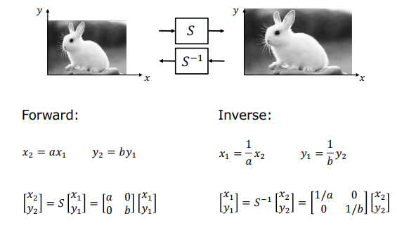
2.2 2D Rotation
To rotate a point $p_1(x_1, y_1)$ counter-clockwise around the origin by angle $\theta$, we express the initial position using polar coordinates. Let $r$ be distance to origin and $\psi$ the initial angle:
$$x_1 = r \cos \psi, \quad y_1 = r \sin \psi$$
Rotating by angle $\theta$, the new point $p_2(x_2, y_2)$ becomes:
$$x_2 = r \cos(\psi + \theta), \quad y_2 = r \sin(\psi + \theta)$$
Expanding using trigonometric addition formulas:
$$x_2 = r(\cos \psi \cos \theta - \sin \psi \sin \theta) = (r \cos \psi) \cos \theta - (r \sin \psi) \sin \theta$$
$$y_2 = r(\sin \psi \cos \theta + \cos \psi \sin \theta) = (r \cos \psi) \sin \theta + (r \sin \psi) \cos \theta$$
Substituting $x_1$ and $y_1$:
$$x_2 = x_1 \cos \theta - y_1 \sin \theta$$
$$y_2 = x_1 \sin \theta + y_1 \cos \theta$$
Represented in linear matrix form using rotation matrix $R$:
$$\begin{bmatrix} x_2 \ y_2 \end{bmatrix} = \begin{bmatrix} \cos \theta & -\sin \theta \ \sin \theta & \cos \theta \end{bmatrix} \begin{bmatrix} x_1 \ y_1 \end{bmatrix}$$
To invert rotation, inverse matrix $R^{-1}$ is applied. Because rotation matrices are orthogonal ($R^{-1} = R^T$), inversion simply negates the angle:
$$R^{-1} = \begin{bmatrix} \cos \theta & \sin \theta \ -\sin \theta & \cos \theta \end{bmatrix}$$
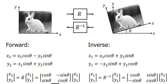
2.3 Skew / Shear
Shear transformations convert rectangular regions into parallelograms.
Horizontal Skew: Shifts the $x$-coordinate proportionally by factor $m$ of vertical position $y$, leaving $y$ unchanged:
$$\begin{bmatrix} x_2 \ y_2 \end{bmatrix} = \begin{bmatrix} 1 & m \ 0 & 1 \end{bmatrix} \begin{bmatrix} x_1 \ y_1 \end{bmatrix}$$
Vertical Skew: Shifts the $y$-coordinate proportionally by factor $m$ of horizontal position $x$, leaving $x$ unchanged:
$$\begin{bmatrix} x_2 \ y_2 \end{bmatrix} = \begin{bmatrix} 1 & 0 \ m & 1 \end{bmatrix} \begin{bmatrix} x_1 \ y_1 \end{bmatrix}$$
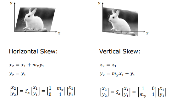
2.4 Mirror / Reflection
Reflection across Y-axis: Negates $x$ coordinates while preserving $y$:
$$\begin{bmatrix} x_2 \ y_2 \end{bmatrix} = \begin{bmatrix} -1 & 0 \ 0 & 1 \end{bmatrix} \begin{bmatrix} x_1 \ y_1 \end{bmatrix}$$
Reflection across line $y = x$ (Diagonal): Swaps $x$ and $y$ coordinate axes:
$$\begin{bmatrix} x_2 \ y_2 \end{bmatrix} = \begin{bmatrix} 0 & 1 \ 1 & 0 \end{bmatrix} \begin{bmatrix} x_1 \ y_1 \end{bmatrix}$$
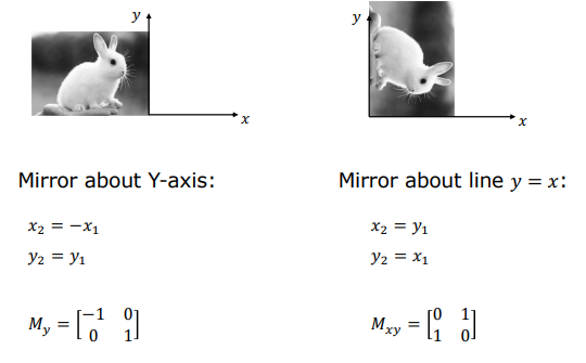
2.5 Properties and Limitations of 2x2 Linear Transformations
- Origin is Invariant: The origin $(0,0)$ always maps to $(0,0)$.
- Lines Map to Lines: Straight lines in input space remain straight lines in output space.
- Parallelism is Preserved: Parallel lines remain strictly parallel after transformation.
- Closed under Composition: Sequential transformations can be combined into a single matrix multiplication:
$$T_{13} = T_{23} \cdot T_{12}$$
Fundamental Limitation of 2x2 Systems (Translation Problem): Translation ($x_2 = x_1 + t_x$ and $y_2 = y_1 + t_y$), despite being the simplest geometric shift, cannot be expressed as a linear $2 \times 2$ matrix operation because $2 \times 2$ multiplication lacks terms for constant additive offsets $+t_x$ and $+t_y$. To overcome this limitation, coordinates are extended by one dimension into Homogeneous Coordinates.
3. 3x3 Image Transformations
3.1 Homogeneous Coordinates
To resolve dimensional constraints and unify translation with linear transformations under a single matrix multiplication, Homogeneous Coordinates are introduced.
A 2D point $p(x,y)$ is represented in homogeneous coordinates by adding a non-zero fictitious scale dimension $\tilde{z}$, forming a 3D point $\tilde{p}(\tilde{x}, \tilde{y}, \tilde{z})$. Mapping back to 2D Cartesian coordinates is defined as:
$$x = \frac{\tilde{x}}{\tilde{z}}, \quad y = \frac{\tilde{y}}{\tilde{z}}$$
Geometrically, the 2D Cartesian plane corresponds to the plane $\tilde{z} = 1$ in 3D homogeneous space. A ray $L$ originating from the origin and passing through $p(x,y,1)$ contains equivalent homogeneous representations of the same 2D point $p(x,y)$.
z_tilde
▲ / Ray L (All points along ray are equivalent)
│ /
1.0 ─┼────────• p(x, y, 1) <-- Projection Plane
│ /│
│ / │
│ / │
│ / │
└───•────┼─────────► x_tilde
Origin │
▼ y_tilde
Consequently, multiplying homogeneous vector $[x, y, 1]^T$ by any non-zero scale factor $\tilde{z}$ yields $[\tilde{z}x, \tilde{z}y, \tilde{z}]^T$, which represents the identical physical 2D point.
3.2 3x3 Representation of Translation
Using homogeneous coordinates, translation becomes a linear $3 \times 3$ matrix multiplication:
$$\begin{bmatrix} x_2 \ y_2 \ 1 \end{bmatrix} = \begin{bmatrix} 1 & 0 & t_x \ 0 & 1 & t_y \ 0 & 0 & 1 \end{bmatrix} \begin{bmatrix} x_1 \ y_1 \ 1 \end{bmatrix} = \begin{bmatrix} x_1 + t_x \ y_1 + t_y \ 1 \end{bmatrix}$$
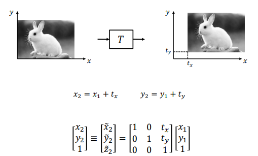
All $2 \times 2$ operations (scaling, rotation, skew) are embedded into the upper-left $2 \times 2$ submatrix of $3 \times 3$ homogeneous matrices. A sequence of transformations (e.g., skew, translate, scale, rotate) can thus be concatenated into a single composite $3 \times 3$ matrix applied in a single pass.
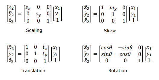
3.3 Affine Transformations
Any $3 \times 3$ homogeneous transformation matrix whose bottom row is fixed to $[0\quad0\quad1]$ belongs to the Affine Transformation class:
$$\begin{bmatrix} x_2 \ y_2 \ 1 \end{bmatrix} = \begin{bmatrix} a_{11} & a_{12} & t_x \ a_{21} & a_{22} & t_y \ 0 & 0 & 1 \end{bmatrix} \begin{bmatrix} x_1 \ y_1 \ 1 \end{bmatrix}$$
Affine transformations possess 6 degrees of freedom (DoF).
Properties of Affine Transformations:
- The origin does not need to map to the origin (translation is supported).
- Lines map to lines.
- Parallel lines remain strictly parallel.
- Closed under composition.
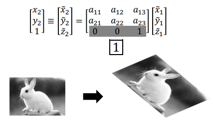
3.4 Projective Transformations (Homography)
When the bottom row of a $3 \times 3$ homogeneous transformation matrix is unconstrained ($[h_{31}, h_{32}, h_{33}]$), the transformation is a Projective Transformation or Homography:
$$\begin{bmatrix} \tilde{x}2 \ \tilde{y}2 \ \tilde{z}2 \end{bmatrix} = \begin{bmatrix} h{11} & h{12} & h{13} \ h_{21} & h_{22} & h_{23} \ h_{31} & h_{32} & h_{33} \end{bmatrix} \begin{bmatrix} x_1 \ y_1 \ 1 \end{bmatrix}$$
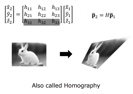
A projective transformation maps points on a plane $\Pi_1$ through a single projection center (pinhole) onto another plane $\Pi_2$. This models the perspective projection geometry of a camera imaging a planar scene.
Scale Ambiguity and Degrees of Freedom: Due to homogeneous equivalence, multiplying homography matrix $H$ by any non-zero scalar $k$ does not alter final Cartesian coordinates $(x_2, y_2)$. Thus, homography is defined only up to a scale factor. Fixing scale via constraint $\sum h_{ij}^2 = 1$ leaves 8 degrees of freedom (DoF) despite having 9 matrix entries.
Properties of Projective Transformations:
- Lines map to lines and composition is closed.
- Key difference from Affine Transformations: Parallel lines are not preserved. Under perspective projection, parallel lines converge toward vanishing points (e.g., railway tracks converging at the horizon).
4. Transformation Properties Summary
| Transformation Type | Matrix Size | Degrees of Freedom (DoF) | Preserved Geometric Properties | Bottom Row Constraint |
|---|---|---|---|---|
| Linear (2x2) | $2 \times 2$ | 4 | Origin, Linearity, Parallelism | - |
| Affine | $3 \times 3$ | 6 | Linearity, Parallelism | $[0 \quad 0 \quad 1]$ |
| Projective (Homography) | $3 \times 3$ | 8 | Linearity | Free (Up to Scale) |
Homography Estimation, RANSAC, Warping and Blending
1. Computing Homography
1.1 Role in Image Stitching
When a camera rotates around its optical center to capture images from different angles, all resulting image planes (e.g., $\Pi_1, \Pi_2, \Pi_3$) share the identical projection center (pinhole). Consequently, points across these image planes are directly linked by homography matrices. By cascading homographies via composition, all images can be seamlessly aligned onto a single reference plane ($\Pi_p$).
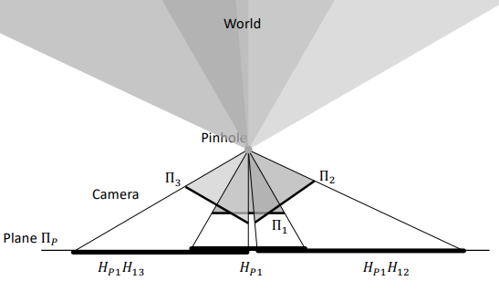
1.2 Conditions of Homography Validity
Homography-based image alignment is mathematically valid in three primary scenarios:
- Same Viewpoint (Pure Rotation): The camera rotates strictly around its optical center without translation. In this case, homography is exact regardless of the 3D scene depth structure.
- Planar Scenes: Even if the camera translates to different positions, homography holds if the scene object itself is planar in 3D space (e.g., a wall painting or building facade).
- Plane at Infinity: When the scene is extremely distant compared to camera displacement (e.g., distant mountain landscapes), the scene behaves as a plane at infinity, preserving homography validity.
Invalid Case (Parallax Artifacts): When a scene is close to the camera, contains complex 3D depth variations, and the camera translates, homography fails, giving rise to parallax errors.
1.3 Direct Linear Transform (DLT)
Let $H$ be the $3 \times 3$ homography matrix mapping a point $p_s[x_s, y_s, 1]^T$ in the source image to point $p_d[x_d, y_d, 1]^T$ in the destination image:
$$p_d \equiv H \cdot p_s$$
$$\begin{bmatrix} \tilde{x}d \ \tilde{y}d \ \tilde{z}d \end{bmatrix} = \begin{bmatrix} h{11} & h{12} & h{13} \ h_{21} & h_{22} & h_{23} \ h_{31} & h_{32} & h_{33} \end{bmatrix} \begin{bmatrix} x_s \ y_s \ 1 \end{bmatrix}$$
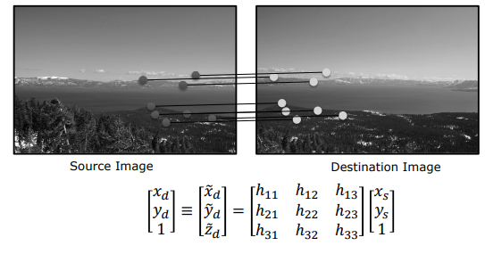
Expanding this linear system and performing homogeneous normalization ($x_d = \tilde{x}_d / \tilde{z}_d$ and $y_d = \tilde{y}_d / \tilde{z}_d$), each point match provides two linear equations:
$$x_d = \frac{h_{11}x_s + h_{12}y_s + h_{13}}{h_{31}x_s + h_{32}y_s + h_{33}}$$
$$y_d = \frac{h_{21}x_s + h_{22}y_s + h_{23}}{h_{31}x_s + h_{32}y_s + h_{33}}$$
Rearranging terms with respect to unknown matrix entries $h_{ij}$:
$$x_s h_{11} + y_s h_{12} + h_{13} - x_d x_s h_{31} - x_d y_s h_{32} - x_d h_{33} = 0$$
$$x_s h_{21} + y_s h_{22} + h_{23} - y_d x_s h_{31} - y_d y_s h_{32} - y_d h_{33} = 0$$
Since each point match provides 2 independent constraints and homography has 8 degrees of freedom, a minimum of 4 point correspondences (minimum 4 pairs) is required to solve $H$.
1.4 Constrained Least Squares Estimation
In practical settings, more than 4 point matches ($N > 4$) are utilized to suppress noise, yielding an overdetermined linear system. Stacking equations for all $N$ pairs produces a $2N \times 9$ coefficient matrix $A$:
$$A \cdot h = 0$$
where $h = [h_{11}, h_{12}, h_{13}, h_{21}, h_{22}, h_{23}, h_{31}, h_{32}, h_{33}]^T$. To prevent the trivial solution $h = 0$, we enforce the scale constraint $|h|^2 = 1$.
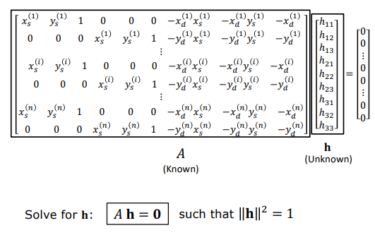
We formulate the optimization problem to minimize $|A \cdot h|^2$ subject to $|h|^2 = 1$:
$$\min_{h} h^T A^T A h \quad \text{subject to} \quad h^T h = 1$$
Adding a Lagrange multiplier $\lambda$ yields the Lagrangian loss function:
$$\mathcal{L}(h, \lambda) = h^T A^T A h - \lambda (h^T h - 1)$$
Taking partial derivatives with respect to $h$ and setting to zero leads to the standard Eigenvalue problem:
$$A^T A h = \lambda h$$
Optimal Solution: The parameter vector $h$ minimizing the error corresponds to the eigenvector associated with the smallest eigenvalue of $A^T A$. Computing Singular Value Decomposition (SVD) $A = U \Sigma V^T$, $h$ is given by the last column of $V$. Reshaping $h$ into $3 \times 3$ yields homography matrix $H$.
2. Dealing with Outliers: RANSAC
2.1 The Outlier Problem
Feature detectors like SIFT identify matches based purely on local descriptor similarity. Repetitive patterns, reflections, or noise inevitably introduce false matches (outliers) that do not represent identical 3D points.
[Inliers (Valid Matches)] [Outliers (False Matches)]
Corresponding 3D points Incorrect pairings caused by
in shared scene space descriptor similarity or noise
If outliers are included in standard least-squares estimation, the estimated transformation matrix is severely distorted. Outliers must be rejected before computing the final homography.
2.2 RANSAC (Random Sample Consensus) Algorithm
RANSAC is a robust consensus algorithm capable of estimating accurate model parameters even when outliers exceed 50% of the dataset.
RANSAC execution steps for homography estimation:
- Randomly select a minimal subset of 4 point matches ($s = 4$).
- Compute candidate homography matrix $H$ from these 4 points via DLT.
- Project all data points using candidate $H$ and measure reprojection error. Matches with reprojection error below threshold $\epsilon$ are classified as Inliers, yielding consensus score $M$.
- Repeat steps 1–3 for $N$ iterations.
- Select the candidate matrix $H$ with the highest consensus score $M$ as the winning model.
Model Refinement: After RANSAC selects the winning model, all identified inliers ($M$ points) are pooled together. Constrained Least Squares is re-executed over the full inlier set to produce a refined, highly accurate homography matrix $H$.
3. Image Warping and Blending
After computing homography $H$, geometric warping and photometric blending operations assemble individual images into a seamless panorama.
3.1 Forward Warping and Hole Artifacts
In forward warping, transformation $H$ is applied to each pixel coordinate $(x_s, y_s)$ in the source image to compute destination coordinate $(x_d, y_d)$, writing source pixel color to that target location.
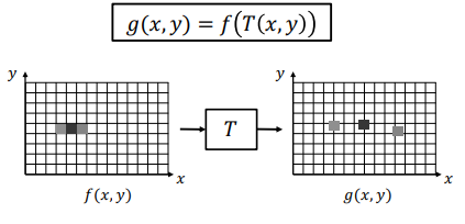
Forward warping suffers from two major drawbacks:
- Non-integer Coordinates: Transformed coordinates rarely align with integer pixel grid centers in the output image.
- Holes and Gaps: Geometric expansion leaves target pixels unmapped by any source pixel, producing unassigned black holes.
3.2 Backward Warping
To eliminate hole artifacts, backward warping is performed:
- Transform the 4 corners of the source image using forward homography to determine output bounding box dimensions.
- Iterate through every integer pixel coordinate $(x_d, y_d)$ within the output canvas.
- Apply inverse homography ($H^{-1}$) to locate source coordinate $(x_s, y_s)$.
- Sample pixel color from the source image at $(x_s, y_s)$ using Bilinear Interpolation or Nearest Neighbor.
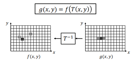
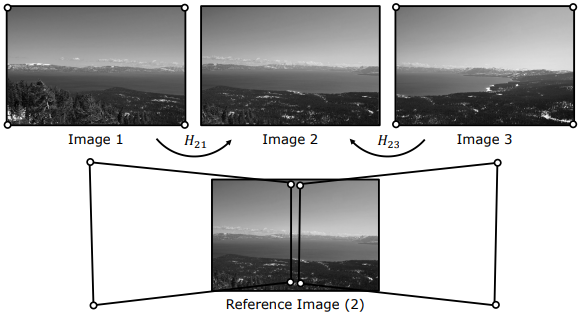
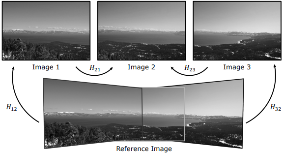
[Forward Warping] (x, y) ──► H ──► (x', y') (Leaves gaps and unassigned holes)
[Backward Warping] (x', y') ──► H^-1 ──► (x, y) (Seamless, gap-free output)
Because every pixel in the output canvas is back-projected and sampled, backward warping guarantees a completely gap-free composite image.
3.3 Image Blending and Seam Artifacts
Even when images are aligned with geometric precision, directly overlaying them creates sharp seam boundaries (hard seams).
Seams arise due to two primary optical factors:
- Exposure and Illumination Variations: Automatic camera exposure adjustments or dynamic ambient lighting changes between shots.
- Vignetting Effects: Lens falloff causing pixel brightness to decrease near image boundaries compared to the center.
Human vision is acutely sensitive to intensity steps as small as 1 gray level across smooth regions. Simple pixel averaging softens transition boundaries but fails to eliminate seams.
3.4 Weighted Blending
To eliminate seam lines, pixel weights are assigned based on spatial proximity to image centers. The blended pixel intensity ($I_{\text{blend}}$) is computed using smooth weight matrices $w_1$ and $w_2$:
$$I_{\text{blend}} = \frac{w_1 I_1 + w_2 I_2}{w_1 + w_2}$$
3.5 Distance Transform-Based Blending
Optimal blending weights are computed using the Distance Transform (e.g., MATLAB bwdist):
- The weight of each pixel is proportional to its Euclidean distance from the nearest image boundary.
- Pixels near the center receive higher weight ($w$), reflecting higher optical quality and lower vignetting falloff. Boundary pixel weights decay smoothly to zero.
Distance transform blending spreads intensity transitions smoothly across overlap regions, producing high-resolution panoramas free of visible seam artifacts.
Face Detection
- 1. Overview
- 2. Uses of Face Detection
- 3. Haar Features
- 4. Integral Image
- 5. Nearest Neighbor Classifier
- 6. Support Vector Machine (SVM)
- 7. Summary & Final Evaluation
1. Overview
Face detection is a fundamental computer vision task that aims to determine the coordinates and extent of all human faces within a digital input image or video stream. The primary output of the detection algorithm is a local search window (bounding box) placed around each detected face.
flowchart TD
Input["Input Image"] --> Scan["Multi-Scale Raster Scan"]
Scan --> Window["Pixel Window (e.g., 24x24)"]
Window --> Haar["Haar Feature Extraction"]
II["Integral Image (II)"] -.->|"Fast O(1) Access"| Haar
Haar --> Classifier["SVM Linear Classifier"]
Classifier --> Face["Face Class (+1)"]
Classifier --> NonFace["Non-Face Class (-1)"]
Face --> NMS["Multi-Window Non-Maximal Suppression (NMS)"]
NMS --> Output["Final Face Bounding Box Output"]
style Input fill:#1a1a2e,stroke:#e94560,color:#fff
style Scan fill:#16213e,stroke:#0f3460,color:#fff
style Window fill:#0f3460,stroke:#e94560,color:#fff
style Haar fill:#1a1a2e,stroke:#4cc9f0,color:#fff
style II fill:#0f3460,stroke:#4cc9f0,color:#fff
style Classifier fill:#16213e,stroke:#e94560,color:#fff
style Face fill:#1b4332,stroke:#52b788,color:#fff
style NonFace fill:#5c1d24,stroke:#e63946,color:#fff
style NMS fill:#1a1a2e,stroke:#4cc9f0,color:#fff
style Output fill:#16213e,stroke:#4cc9f0,color:#fff

1.1 Key Challenges in Face Detection
A robust face detection system must tolerate significant physical variations:
- Scale Invariance: Due to varying distances from the camera, facial bounding box sizes change continuously. The system must scan windows across multiple scale spaces.
- Illumination Invariance: Distinct facial geometry must remain detectable under diverse lighting conditions, specular highlights, and harsh shadows.
- Pose Tolerance: Slight in-plane tilts or out-of-plane head rotations (pose) must not collapse detection quality. To simplify initial theory, algorithms initially focus on frontal head-on faces.
1.2 Limitations & Comparison of Other Feature Models
The choice of visual features dictates both system execution speed and classification accuracy. Traditional feature representations exhibit distinct shortcomings in face detection:
- Edges and Corners: A massive number of edge/corner pixels are produced by background clutter and image noise. Their discriminative power for defining complex face morphology is very low.
- SIFT (Scale-Invariant Feature Transform): SIFT excels at matching identical local patches across different views of a specific object instance (appearance matching). However, face detection is not instance recognition; its goal is to draw general class decision boundaries between face vs. non-face patterns. Because human faces vary greatly across identities and expressions, SIFT fails to generalize efficiently for detection.
- Facial Component Templates: Designing independent templates for facial sub-components (eyes, nose, mouth) and searching via cross-correlation (template matching) suffers from high shape variability within components (especially eyes), yielding historically limited success.
Key Insight: Because face detection is evaluated billions of times across every pixel and scale of an image, the chosen features must be both highly discriminative and extremely fast to compute. The visual representation satisfying both criteria is Haar Features.
2. Uses of Face Detection
Face detection serves as an essential precursor step across modern commercial and industrial applications:
- Smartphone Cameras & Mobile Photography: Opening a phone camera triggers real-time face detection. Hardware parameters such as autofocus, automatic exposure (AE), and color balance are dynamically adjusted to optimize the rendering quality of detected face regions.
- Visual Search Engines: Searching for “gates” in a search engine returns physical gates as well as people like Bill Gates. Filtering by “Face” executes background face detection to isolate images containing human faces.
- Demographic Analytics & Intelligent Marketing: Used in retail and public spaces to analyze customer demographics. For instance, digital vending machines at Shinagawa Station in Japan detect a customer’s face to estimate gender and age (within a 5-year margin). Based on this demographic profile, targeted product recommendations are dynamically displayed. Additionally, shopping mall attention mapping uses face detection to price digital billboards.
- Biometrics, Security & Surveillance: Serving as the foundational first step for access control systems, crowd density monitoring, and real-time suspect identification in public or private security camera networks.
3. Haar Features
Haar Features used in face detection are two-valued filter masks based on 2D Haar Wavelet theory and rectangular box functions.
3.1 Principle & Mathematical Definition
Each Haar filter consists of adjacent white (+1 weight) and black (-1 weight) rectangular regions placed within a local analysis window.
Physically, sliding a Haar filter across an image computes a cross-correlation operation. Standard correlation requires multiplying pixel values by filter weights and summing them up. However, because Haar weights are strictly $+1$ and $-1$, the operation simplifies entirely to pure additions and subtractions, completely bypassing multiplications:
$$\text{Haar Response} = \sum_{(x,y) \in \text{White}} I(x,y) - \sum_{(x,y) \in \text{Black}} I(x,y)$$
where $I(x,y)$ represents original pixel intensity values. Eliminating multiplications provides an immense computational advantage for hardware processors (CPUs/GPUs).
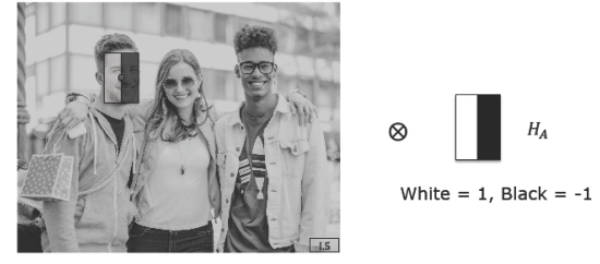
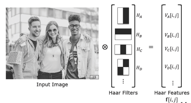
3.2 Haar Filter Types & Derivative Analogy
Haar filter banks are structured into scales and orientations to extract diverse geometric patterns:
- Two-Rectangle Filters (Vertical/Horizontal): A vertical filter with white on the left and black on the right captures sharp horizontal intensity transitions. It acts analogously to a first-order derivative (gradient) operator and functions as a large-scale edge detector.
- Three-Rectangle Filters (e.g., White-Black-White): Filters with a central black strip flanked by white rectangles simulate a second-order derivative (Laplacian) operator, detecting line and ridge structures.
- Complex Multi-Rectangle Filters: Four-rectangle diagonal patterns represent higher-order partial derivatives, capturing complex texture transitions.
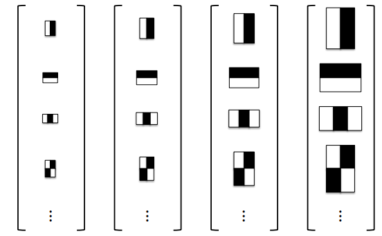
3.3 Standard Computation Cost
For a standard image patch, computing the response of a single $N \times M$ Haar filter directly requires:
$$\text{Number of Addition Operations} = (N \times M) - 1$$
Although multiplication-free, evaluating this for millions of image pixels across dozens of scales and hundreds of feature templates creates a massive computational bottleneck, preventing real-time performance. This challenge is overcome using the Integral Image.
4. Integral Image
An Integral Image (Summed-Area Table) is an intermediate image representation that enables computing the sum of pixel values within any rectangular sub-region in $O(1)$ constant time, independent of rectangle size.
4.1 Mathematical Definition
For an original image $I(x,y)$, the integral image $II(x,y)$ stores the sum of all pixels above and to the left of $(x,y)$, inclusive:
$$II(x,y) = \sum_{x’ \le x, , y’ \le y} I(x’,y’)$$
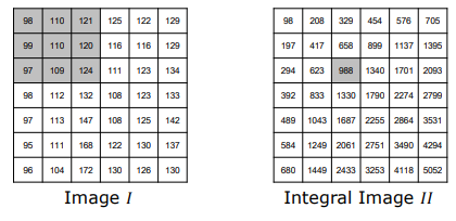
4.2 Single-Pass Raster Construction
The integral image is constructed in a single raster scan over the image ($O(N)$ complexity). The integral value at coordinate $O(x,y)$ is computed recursively using its left neighbor ($A$), top neighbor ($B$), and top-left diagonal neighbor ($C$):
$$II(O) = II(A) + II(B) - II(C) + I(O)$$
Logic / Proof: Summing the top region ($II(B)$) and left region ($II(A)$) double-counts their intersection area ($II(C)$). Subtracting $II(C)$ once corrects this double counting before adding the current pixel value $I(O)$.
4.3 $O(1)$ Constant Time Rectangle Sum Calculation
Once built, the pixel sum inside any target rectangle $D$ bounded by vertices $P, Q, R, S$ requires only 4 array lookups and 3 arithmetic operations:
$$\text{Rectangle Sum} = II(P) - II(Q) - II(S) + II(R)$$
Explanation: Bottom-right vertex $II(P)$ gives the total sum of the entire top-left region. Subtracting top strip $II(Q)$ and left strip $II(S)$ removes non-target regions. Because intersection region $II(R)$ was subtracted twice, adding $II(R)$ back restores exact balance.
This calculation cost is strictly constant ($O(1)$) whether the rectangle spans $3 \times 3$ or $300 \times 300$ pixels.
4.4 Application to Haar Features & Computational Speedup
A two-rectangle Haar feature (one black, one white region) is modeled as two adjacent rectangles:
- White region sum is obtained using 4 corner lookups ($O, T, R, S$).
- Black region sum is obtained using 4 corner lookups ($P, Q, T, O$).
Subtracting the two region sums cancels out shared border vertices:
$$\text{Haar Response} = (II(O) - II(T) + II(R) - II(S)) - (II(P) - II(Q) + II(T) - II(O))$$
After simplification, any Haar feature response is evaluated in exactly 7 addition/subtraction operations. This constant-time evaluation provides dramatic acceleration for multi-scale face detection.
5. Nearest Neighbor Classifier
After extracting Haar feature vectors from candidate windows, a classification model determines whether the vector represents a face or non-face.
5.1 Principle
A training dataset of thousands of labeled face and non-face image patches is collected. An $N$-element Haar feature vector is represented as a point in $N$-dimensional feature space.
In a Nearest Neighbor (NN) classifier:
- A candidate window feature vector is computed and positioned in $N$-dimensional space.
- Geometric Euclidean distances to all stored training samples are computed.
- The label of the closest training point (closest neighbor) is retrieved.
- The test window is assigned the retrieved class label (Face or Non-Face).
5.2 False Positives & Dataset Expansion
If a non-face test pattern resembles facial geometry (e.g., a cat face or unaligned partial feature), its vector may fall near the face cluster, causing a false positive.
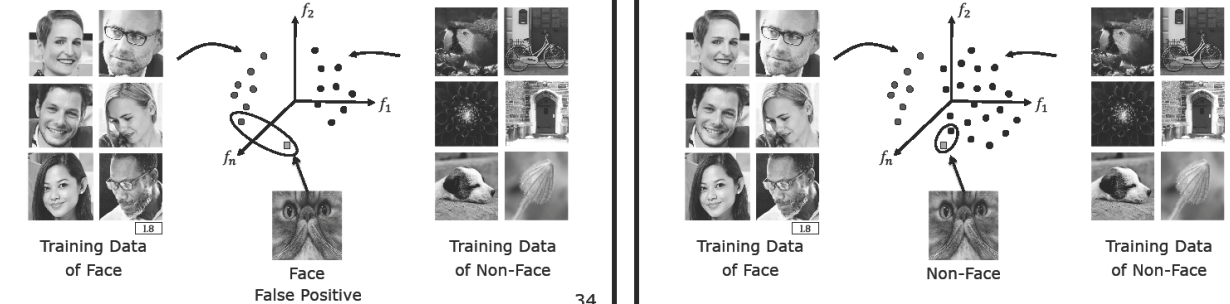
The direct resolution is expanding the training dataset—particularly with diverse non-face examples. Densely surrounding non-face geometric outliers with non-face labels prevents misclassifications.
5.3 Computational Bottleneck & Need for Decision Boundaries
However, scaling training data creates severe latency issues. A brute-force NN classifier evaluates test points against every stored training sample ($O(N \cdot d)$ time). Even with indexing trees (K-D Trees), performing exhaustive point searches across millions of windows per frame is computationally prohibitive.
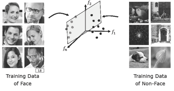
Key Insight: To eliminate linear scan overhead, instead of searching individual database points, geometric Decision Boundaries are placed between face and non-face clusters. Once a decision boundary is established, evaluating a new point requires only checking which side of the boundary hyperplane it lies on.
6. Support Vector Machine (SVM)
A Support Vector Machine (SVM) computes the mathematically optimal linear decision boundary separating face and non-face feature clusters while maximizing geometric margins.
6.1 Geometric Formulation of Linear Decision Boundaries
The dimensionality of feature space determines the boundary geometry:
- 2D Space: The boundary is a 1D line.
- 3D Space: The boundary is a 2D plane.
- N-D Space: The boundary is an $(N-1)$-dimensional hyperplane.
In all dimensions, the hyperplane is expressed in vector form:
$$\mathbf{w}^T \mathbf{f} + b = 0$$
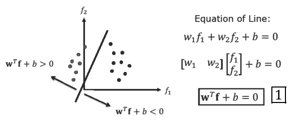
where:
- $\mathbf{w}$: Weight vector defining hyperplane orientation and coefficients.
- $\mathbf{f}$: Input Haar feature vector.
- $b$: Scalar bias (intercept) parameter.
For a query vector $\mathbf{f}$, the sign of the hyperplane equation yields the class:
- If $\mathbf{w}^T \mathbf{f} + b > 0 \rightarrow$ Classified as Face (+1).
- If $\mathbf{w}^T \mathbf{f} + b < 0 \rightarrow$ Classified as Non-Face (-1).
6.2 Safe Zone & Margin ($\rho$)
Infinitely many hyperplanes can separate linearly separable training sets. Selecting an arbitrary boundary risks poor generalization on unseen data.
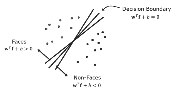
To maximize stability, a safe zone of total thickness margin ($\rho$) is constructed around the decision boundary. The margin represents the maximum width the boundary strip can expand before contacting training points.
SVM optimizes: Maximizing the margin thickness ($\rho$) separating face (+1) and non-face (-1) classes (maximum margin classification).
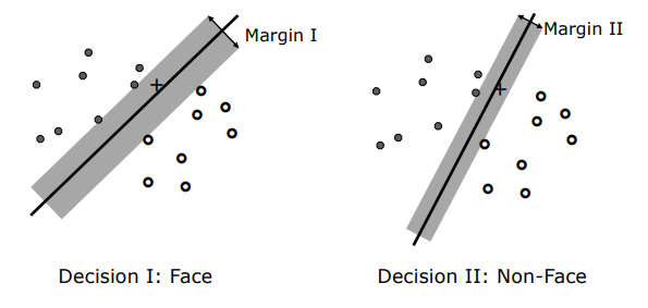
6.3 Support Vectors
Training points touching the outer boundaries of the safe zone are called Support Vectors.
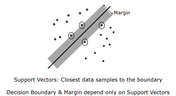
Key Insight: The optimal decision hyperplane depends exclusively on support vectors. Once calculated, all other training points outside the safe zone boundary can be safely discarded, drastically reducing memory footprint and prediction latency.
6.4 Mathematical Optimization & Constraints
For $k$ training vectors $\mathbf{f}_i$ with labels $\lambda_i \in {+1, -1}$:
- Face points ($\lambda_i = +1$): $\mathbf{w}^T \mathbf{f}_i + b \geq \frac{\rho}{2}$
- Non-face points ($\lambda_i = -1$): $\mathbf{w}^T \mathbf{f}_i + b \leq -\frac{\rho}{2}$
Combined constraint formulation:
$$\lambda_i \left( \mathbf{w}^T \mathbf{f}_i + b \right) \geq \frac{\rho}{2}$$
For support vectors $\mathbf{f}_s$, the constraint holds with strict equality: $\lambda_s (\mathbf{w}^T \mathbf{f}_s + b) = \frac{\rho}{2}$. Convex quadratic optimization algorithms solve for optimal parameters $\mathbf{w}$ and $b$.
6.5 Classifying New Data Points
For a new window feature vector $\mathbf{f}$, signed distance $d$ to the decision boundary is computed:
$$d = \mathbf{w}^T \mathbf{f} + b$$
Classification rules:
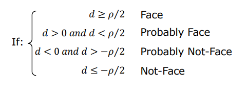
- $d \ge \frac{\rho}{2} \rightarrow$ Outside safe zone on face side; Definitely Face.
- $d \le -\frac{\rho}{2} \rightarrow$ Outside safe zone on non-face side; Definitely Non-Face.
- $0 < d < \frac{\rho}{2} \rightarrow$ Inside safe zone on face side; Probably Face.
- $-\frac{\rho}{2} < d < 0 \rightarrow$ Inside safe zone on non-face side; Probably Not Face.
6.6 Non-Maximal Suppression (NMS)
Scanning a video frame produces multiple overlapping bounding box detections around a single face because neighboring window offsets also pass the classifier threshold. Non-Maximal Suppression (NMS) merges overlapping candidate bounding boxes, retaining only the highest-scoring detection window.
7. Summary & Final Evaluation
- Mature Technology: Face detection represents a mature computer vision technology deployed pervasively across consumer devices and security infrastructure.
- Handling Pose Variations: Frontal models struggle with profile views. Systems integrate multi-pose models (e.g., dedicated classifiers trained for 30–60° or full profile angles).
- Surpassing Human Performance: Modern face recognition systems built atop face detection pipelines exceed human visual recognition accuracy on benchmark evaluation datasets.
Overview, Radiometric Concepts, Radiance, and BRDF
- 1. Overview: The Image Intensity Understanding Problem
- 2. Radiometric Concepts
- 3. Scene Radiance & Image Irradiance Relationship
- 4. Bidirectional Reflectance Distribution Function (BRDF)
1. Overview: The Image Intensity Understanding Problem
One of the most fundamental physical questions in computer vision is: What does the measured intensity value of a single pixel (e.g., brightness 65) tell us about the corresponding physical point in the scene? This challenge is known as the image intensity understanding problem.
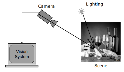
Three main physical factors determine the intensity value of a pixel and make this process complex:
- Illumination: The number, type (point, area, or extended sources like the sky), brightness, and directions of light sources ($\mathbf{s}$).
- Surface Orientation: The three-dimensional surface normal vector ($\mathbf{n}$) at the point of interest.
- Surface Reflectance: The capability of the material to receive light from a specific incident direction and reflect it toward the camera direction (material properties).
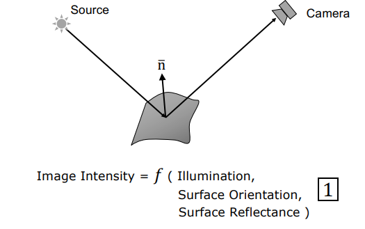
flowchart TD
subgraph Factors["Factors Determining Image Intensity"]
Illum["Illumination (s)<br/>Light source direction & intensity"]
Orient["Surface Orientation (n)<br/>Surface normal vector"]
Reflect["Surface Reflectance<br/>Material reflectance model (BRDF)"]
end
Illum --> Point["Scene Point (dAs)"]
Orient --> Point
Reflect --> Point
Point -->|Pixel Intensity I| Cam["Camera / Observer (v)"]
style Point fill:#1a1a2e,stroke:#e94560,color:#fff
style Cam fill:#16213e,stroke:#4cc9f0,color:#fff
style Illum fill:#0f3460,stroke:#e94560,color:#fff
style Orient fill:#0f3460,stroke:#4cc9f0,color:#fff
style Reflect fill:#0f3460,stroke:#e94560,color:#fff
While we have only a single measurement value (pixel intensity $I$) on the image side, we have numerous unknown variables on the scene side (illumination parameters, surface orientation, and reflectance coefficients). Consequently, the image intensity understanding problem is severely under-constrained.
Key Insight: Although inferring 3D shape and reflectance from a single pixel brightness seems impossible, applying physical laws of light propagation and surface reflectance constraints renders this under-constrained problem mathematically solvable.
2. Radiometric Concepts
Radiometry is the science of measuring electromagnetic radiation (including visible light). The key radiometric concepts used in computer vision to interpret pixel intensities are defined below:
2.1 2D Angle
On a circle, the angle $d\theta$ subtended by an arc length $dl$ from the center is defined as the arc length divided by the radius $r$:
$$d\theta = \frac{dl}{r}$$
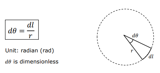
The unit is radians (rad), which is dimensionless since it is a ratio of two lengths. A full circle subtends $2\pi$ radians.
2.2 3D Solid Angle
In 3D space, when viewed from a point $P$, the solid angle subtended by an infinitesimal area $dA$ at distance $r$ considers the slant angle $\theta$ relative to the line of sight. The foreshortened area is calculated as $dA’ = dA \cos\theta$.
The solid angle $d\omega$ is defined as:
$$d\omega = \frac{dA’}{r^2} = \frac{dA \cos\theta}{r^2}$$
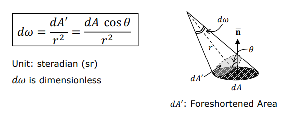
The unit is steradians (sr), which is also dimensionless. Geometric integration yields:
- Total solid angle subtended by a hemisphere: $2\pi \text{ sr}$
- Total solid angle subtended by a full sphere: $4\pi \text{ sr}$
2.3 Radiant Flux ($\Phi$)
Radiant flux is the total electromagnetic power emitted by a light source or received by a surface per unit time. Its unit is Watts (W):
$$\Phi = \frac{dQ}{dt}$$
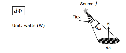
2.4 Radiant Intensity ($J$)
Radiant intensity is the flux emitted by a point light source per unit solid angle in a specific direction $d\omega$:
$$J = \frac{d\Phi}{d\omega}$$
Measured in Watts per steradian (W/sr), this quantity represents the directional brightness of a point light source.
2.5 Surface Irradiance ($E$)
Surface irradiance is the total radiant flux incident per unit surface area:
$$E = \frac{d\Phi}{dA}$$
Its unit is Watts per square meter ($\text{W/m}^2$). For a point source of radiant intensity $J$ at distance $r$ with surface normal inclined by angle $\theta$, surface irradiance is given by:
$$E = \frac{J \cos\theta}{r^2}$$
This equation expresses two fundamental physical laws:
- Inverse Square Law ($1/r^2$ Fall-off): Irradiance decreases inversely with the square of the distance from the light source.
- Cosine Dependence (Lambert’s Cosine Law): As the slant angle $\theta$ increases, the effective area capturing the flux shrinks and irradiance decreases. Irradiance is maximal when light hits perpendicularly ($\theta = 0^\circ$) and drops to zero at glancing incidence ($\theta = 90^\circ$).
2.6 Surface Radiance ($L$)
Surface radiance measures the brightness of light emitted, reflected, or transmitted from a surface point in a specific direction. To remove geometric artifacts such as sensor distance (shrinking solid angle) and expanding surface patch area, radiance is defined as the flux per unit solid angle per unit foreshortened area:
$$L = \frac{d^2\Phi}{d\omega \cdot \cos\theta_r , dA}$$
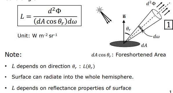
Measured in $\text{W} / (\text{m}^2 \cdot \text{sr})$, radiance depends on the observation direction ($\theta_r$) and varies directionally according to the material’s reflectance properties.
3. Scene Radiance & Image Irradiance Relationship
One of the fundamental physical formulations in computer vision links the scene radiance ($L$) emitted by a scene patch to the image irradiance ($E$) received at the corresponding pixel on the image plane.
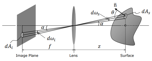
flowchart LR
ScenePatch["Scene Patch (dAs)<br/>Radiance: L<br/>Normal angle: θ"] -->|Flux to Lens dΦ| Lens["Lens (Diameter: d)<br/>Depth: z"]
Lens -->|Focal length: f<br/>Off-axis angle: α| ImagePixel["Image Pixel (dAi)<br/>Irradiance: E"]
style ScenePatch fill:#1a1a2e,stroke:#e94560,color:#fff
style Lens fill:#16213e,stroke:#4cc9f0,color:#fff
style ImagePixel fill:#0f3460,stroke:#e94560,color:#fff
Consider a single-lens camera system with effective focal length $f$ and lens diameter $d$. A pixel of area $dA_i$ on the image plane views a surface patch of area $dA_s$ in the scene along rays passing through the optical center. The surface normal makes an angle $\theta$ with the line of sight, while the line of sight makes an angle $\alpha$ with the optical axis. The depth of the patch is $z$.
Four fundamental equations are established in this geometry:
Equation 1: Solid Angle Equality
The solid angles subtended by the pixel and scene patch at the lens center are equal ($d\omega_i = d\omega_s$):
$$\frac{dA_i \cos\alpha}{(f / \cos\alpha)^2} = \frac{dA_s \cos\theta}{(z / \cos\alpha)^2} \implies \frac{dA_s}{dA_i} = \frac{z^2 \cos\alpha}{f^2 \cos\theta}$$
Equation 2: Lens Solid Angle
The solid angle subtended by the lens when viewed from the scene point is the projected lens area over distance squared:
$$d\omega_l = \frac{\frac{\pi d^2}{4} \cos\alpha}{(z / \cos\alpha)^2} = \frac{\pi d^2 \cos^3\alpha}{4 z^2}$$
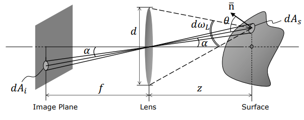
Equation 3: Radiant Flux Collected by Lens
The radiant flux emitted by the scene patch and captured by the lens is expressed using the radiance definition:
$$d\Phi = L \cdot dA_s \cos\theta \cdot d\omega_l$$
Equation 4: Image Irradiance
Since all flux entering the lens falls on the corresponding pixel area, image irradiance is flux over pixel area:
$$E = \frac{d\Phi}{dA_i}$$
The Image Irradiance Equation
Substituting and simplifying these four equations yields the fundamental Image Irradiance Equation:
$$E = L \cdot \frac{\pi}{4} \left(\frac{d}{f}\right)^2 \cos^4\alpha$$
flowchart TD
Eq1["Equation 1:<br/>dAs / dAi Area Ratio"] --> Sub["Substitution & Simplification"]
Eq2["Equation 2:<br/>dωl Lens Solid Angle"] --> Sub
Eq3["Equation 3:<br/>dΦ Collected Flux"] --> Sub
Eq4["Equation 4:<br/>E = dΦ / dAi Irradiance"] --> Sub
Sub --> Final["Image Irradiance Equation:<br/>E = L * (π/4) * (d/f)^2 * cos^4(α)"]
style Eq1 fill:#0f3460,stroke:#4cc9f0,color:#fff
style Eq2 fill:#0f3460,stroke:#4cc9f0,color:#fff
style Eq3 fill:#0f3460,stroke:#4cc9f0,color:#fff
style Eq4 fill:#0f3460,stroke:#4cc9f0,color:#fff
style Final fill:#1a1a2e,stroke:#e94560,color:#fff
Critical Physical Takeaways:
- Linearity: Image irradiance ($E$) is directly proportional to scene radiance ($L$) ($E \propto L$).
- Vignetting ($\cos^4\alpha$ Fall-off): As the angle $\alpha$ off the optical axis increases, image irradiance drops by $\cos^4\alpha$. This physical drop-off is mitigated via compound lens design or digital calibration.
- Depth Independence: The depth parameter $z$ does not appear in the final equation! Moving the camera further away increases the scene area $dA_s$ viewed by a pixel proportional to $z^2$. Simultaneously, the solid angle $d\omega_l$ of the lens shrinks proportional to $1/z^2$. These two effects cancel out perfectly, making image irradiance completely independent of scene depth.
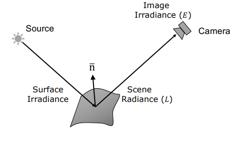
4. Bidirectional Reflectance Distribution Function (BRDF)
The manner in which a surface reflects incoming light depends on atomic and structural material properties. To model this in a general mathematical framework, the BRDF (Bidirectional Reflectance Distribution Function) is used.
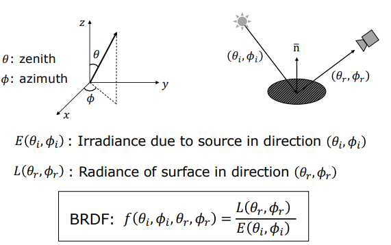
flowchart TD
LightSource["Illumination Direction (s)<br/>(θi, φi)"] -->|Incident Surface Irradiance dEi| Point["Surface Point & Normal (n)"]
Point -->|Reflected Surface Radiance dLr| Camera["Observation Direction (v)<br/>(θr, φr)"]
style LightSource fill:#0f3460,stroke:#e94560,color:#fff
style Point fill:#1a1a2e,stroke:#4cc9f0,color:#fff
style Camera fill:#16213e,stroke:#e94560,color:#fff
BRDF is parametrized using a bidirectional geometry:
- Incident (illumination) direction: $(\theta_i, \phi_i)$
- Reflected (observation) direction: $(\theta_r, \phi_r)$
These directions are specified using zenith angle ($\theta$) and azimuth angle ($\phi$).
4.1 Mathematical Definition
The BRDF ($f$) is a 4-dimensional function defined as the ratio of reflected surface radiance ($L$) in the observation direction to the incident surface irradiance ($E$):
$$f(\theta_i, \phi_i, \theta_r, \phi_r) = \frac{L(\theta_r, \phi_r)}{E(\theta_i, \phi_i)}$$
Its unit is $\text{sr}^{-1}$ (inverse steradians).
4.2 Key Physical Properties of BRDF
The BRDF function satisfies three key physical principles:
-
Non-Negativity: Since energy cannot be negative, BRDF is strictly non-negative: $$f \ge 0$$
-
Helmholtz Reciprocity: Swapping the light source and observer positions leaves the BRDF value unchanged: $$f(\theta_i, \phi_i, \theta_r, \phi_r) = f(\theta_r, \phi_r, \theta_i, \phi_i)$$
-
Isotropy vs. Anisotropy:
- Isotropic: Homogeneous materials (such as matte paint or ceramic) do not change brightness when rotated around the surface normal. For these materials, BRDF dimensionality reduces to 3D as it depends only on the azimuth angle difference: $$f(\theta_i, \theta_r, \phi_r - \phi_i)$$
- Anisotropic: Materials with oriented microstructures (brushed metals, velvet fabric, butterfly wings, peacock feathers) exhibit directional behavior. Rotating the surface about its normal changes its brightness dramatically, so their BRDF remains 4-dimensional.
Reflectance Models, Rough Surfaces, and Dichromatic Model
1. Reflectance Models
Reflection processes in nature are explained primarily by the combination of two physical mechanisms:
- Surface (Specular) Reflection: Light reflects directly at the material interface without entering the bulk medium. It dominates on smooth metals, glass, and mirrors, giving objects a glossy appearance.
- Body (Diffuse) Reflection: Light penetrates the surface, undergoes multiple internal refractions and scattering off heterogeneous particles inside the material, and exits in random directions. It dominates on clay, plaster, and paper, producing a matte appearance.
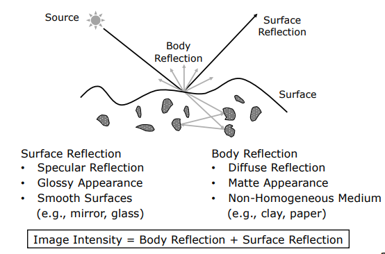
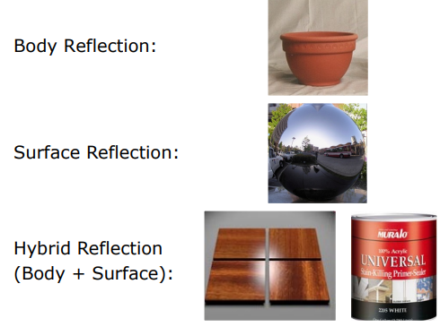
flowchart TD
IncidentLight["Incident Light Energy"] --> SurfaceRefl["Surface Reflection (Specular)<br/>Direct Interface Reflection<br/>Glossy / Mirror-like Appearance"]
IncidentLight --> BodyRefl["Body Reflection (Diffuse)<br/>Internal Scattering & Random Outflow<br/>Matte Appearance"]
SurfaceRefl --> Combined["Total Measured Pixel Intensity<br/>I = I_surface + I_body"]
BodyRefl --> Combined
style IncidentLight fill:#0f3460,stroke:#e94560,color:#fff
style SurfaceRefl fill:#16213e,stroke:#4cc9f0,color:#fff
style BodyRefl fill:#16213e,stroke:#4cc9f0,color:#fff
style Combined fill:#1a1a2e,stroke:#e94560,color:#fff
1.1 Lambertian Model (Body Reflection)
Modeling ideal matte surfaces, the Lambertian model assumes that a surface appears equally bright regardless of the viewing direction (radiance is independent of observation angle). Its BRDF is constant:
$$f_{\text{Lambertian}} = \frac{\rho_d}{\pi}$$
where $\rho_d$ is the material albedo ($0 \leq \rho_d \leq 1$; 0 for perfectly black, 1 for perfectly white).
The radiance equation for a Lambertian surface is given by:
$$L = \frac{\rho_d}{\pi} E = \frac{\rho_d}{\pi} \frac{J}{r^2} (\mathbf{n} \cdot \mathbf{s})$$
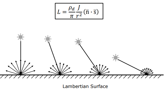
where $\mathbf{s}$ is the unit vector pointing toward the light source and $\mathbf{n}$ is the surface normal unit vector. Radiance is independent of viewing direction, depending only on the cosine of the illumination angle ($\mathbf{n} \cdot \mathbf{s}$).
1.2 Ideal Specular Model
Modeling perfect mirrors, this system reflects all incident light energy into a single reflection direction ($\mathbf{r}$). An observer views light only when the viewing direction ($\mathbf{v}$) perfectly aligns with this direction ($\mathbf{v} = \mathbf{r}$).
The BRDF is expressed using Dirac Delta functions:
$$f_{\text{Specular}} = \frac{\delta(\theta_r - \theta_i) \delta(\phi_r - (\phi_i + \pi))}{\cos\theta_i \sin\theta_i}$$
where the denominator term serves as a normalization factor to satisfy energy conservation.
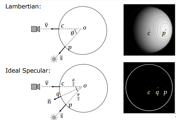
2. Reflection from Rough Surfaces
Real-world surfaces are not perfectly smooth. At the pixel micro-scale, a surface consists of microscopic planar facets (microfacets) facing various directions. Microfacet normal orientations ($\alpha$ angles) are modeled using a Gaussian distribution $p(\alpha, \sigma)$ with standard deviation roughness parameter $\sigma$.
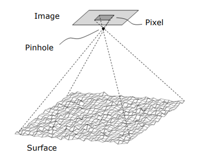
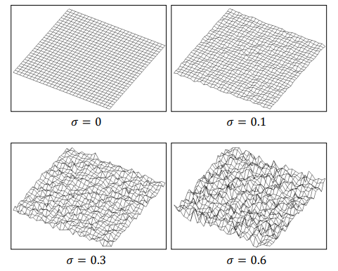
flowchart LR
MacroNormal["Macro Surface Normal (n)"] --> MicroFacets["Microfacets (n_i)"]
GaussDist["Gaussian Distribution p(α, σ)<br/>Roughness Parameter: σ"] --> MicroFacets
MicroFacets --> SpecularLobe["Specular Rough:<br/>Torrance-Sparrow Model"]
MicroFacets --> DiffuseLobe["Diffuse Rough:<br/>Oren-Nayar Model"]
style MacroNormal fill:#0f3460,stroke:#4cc9f0,color:#fff
style GaussDist fill:#0f3460,stroke:#4cc9f0,color:#fff
style SpecularLobe fill:#1a1a2e,stroke:#e94560,color:#fff
style DiffuseLobe fill:#1a1a2e,stroke:#e94560,color:#fff
2.1 Specular Rough Surfaces: Torrance-Sparrow Model
Assuming that each microfacet acts as an ideal mirror, the overall surface BRDF is derived as:
$$f_{\text{Torrance-Sparrow}} = \frac{\rho_s}{(\mathbf{n} \cdot \mathbf{s})(\mathbf{n} \cdot \mathbf{v})} p(\alpha, \sigma) G(\mathbf{s}, \mathbf{n}, \mathbf{v})$$
- $\rho_s$: Microfacet reflectance capacity.
- $p(\alpha, \sigma)$: Gaussian roughness distribution.
- $G(\mathbf{s}, \mathbf{n}, \mathbf{v})$: Geometrical attenuation factor accounting for inter-facet shadowing and masking.
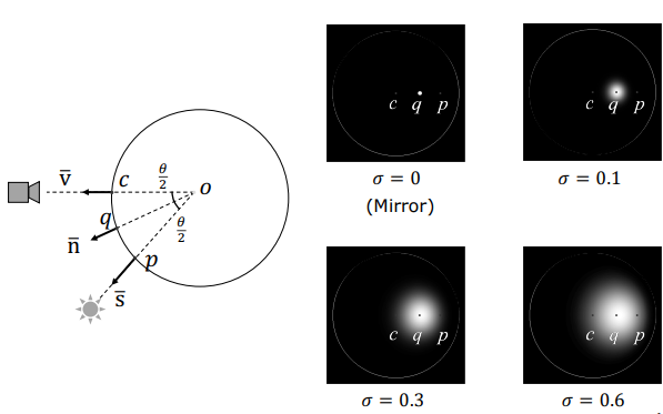
As roughness ($\sigma$) increases, a point specular reflection spreads out into a blurry specular lobe / highlight. For very rough surfaces, the shift of peak brightness away from the perfect specular angle (off-specular peak) is mathematically explained by this model.
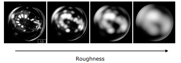
2.2 Diffuse Rough Surfaces: Oren-Nayar Model
Assuming each microfacet is an ideal Lambertian diffuse surface, the model reduces to pure Lambertian when $\sigma = 0$.
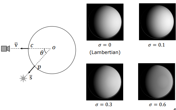
However, as roughness ($\sigma$) increases, rapid brightness drop-off near object edges is prevented, causing spherical objects to appear like flat discs (flat disc phenomenon).
Key Insight: The physical and mathematical explanation for why the full moon appears as a flat disk with uniform brightness up to its limbs—rather than a shaded sphere—is provided by the Oren-Nayar Diffuse Roughness Model.
3. Dichromatic Model
Proposed by Shafer (1985), the Dichromatic Model accounts for light-material color interactions on hybrid dielectric surfaces.
- Surface (Specular) Color Component ($\mathbf{C}_s$): Since light reflects directly at the interface without selective wavelength absorption, specular reflection retains the color of the light source.
- Body (Diffuse) Color Component ($\mathbf{C}_b$): Light entering the medium interacts with pigments, absorbing specific wavelengths. Thus, diffuse reflection color equals the product of illumination color and material pigment color.
The total measured RGB pixel color vector is expressed linearly as:
$$\mathbf{C} = m_b \mathbf{C}_b + m_s \mathbf{C}_s$$
- $\mathbf{C}_b$: Diffuse (body) color vector.
- $\mathbf{C}_s$: Specular (surface) color vector.
- $m_b, m_s$: Geometric weighting parameters.
3.1 Dichromatic Plane & “Skewed-T” Distribution
For an object composed of a single homogeneous material, all pixel color values must lie within the dichromatic plane spanned by $\mathbf{C}_b$ and $\mathbf{C}_s$ in RGB space.
Mapping pixels in color space forms a characteristic “Skewed-T” distribution: one line extending from shadow toward pure body color, and a second line bending toward the light source color at specular highlights.
3.2 Klinker Highlight Separation Algorithm
By analyzing this Skewed-T geometry in RGB space, algorithms developed by Klinker (1990) separate image pixels into a pure diffuse shading image and a pure specular highlight image.
Key Insight: The Klinker highlight separation algorithm eliminates misleading 3D shape artifacts caused by specular highlights, enabling robust recovery of true object geometry and albedo in computer vision.
Overview, Gradient Space, Reflectance Map, and Lambertian Case
- 1. Overview
- 2. Gradient Space and Reflectance Map
- 3. Resolving Ambiguity via Intersection in Photometric Stereo
- 4. Lambertian Case
1. Overview
Interpreting the three-dimensional world from a single two-dimensional image (such as recovering depth) has always been an under-constrained / ill-posed problem in computer vision. Single-image approaches like Shape from Shading attempt to infer the two-dimensional surface gradient ($p, q$) from a single pixel intensity, yielding an infinite set of candidate solutions (infinite ambiguity).
To overcome this fundamental limitation, Photometric Stereo, introduced by Robert Woodham (1980), presents a revolutionary technique for 3D shape reconstruction in controlled illumination environments (such as industrial scanners and quality control systems).
flowchart TD
subgraph Setup["Photometric Stereo Setup"]
Cam["Fixed Camera (x, y)"]
Obj["Fixed Object"]
L1["Light Source 1 (s1)"]
L2["Light Source 2 (s2)"]
L3["Light Source 3 (s3)"]
end
L1 -->|Image I1| Obj
L2 -->|Image I2| Obj
L3 -->|Image I3| Obj
Obj -->|Co-registered Pixels| Cam
Cam -->|Pixel Intensity Variation| Normal["Surface Normal (n) & Albedo (ρ)"]
style Cam fill:#1a1a2e,stroke:#4cc9f0,color:#fff
style Obj fill:#16213e,stroke:#e94560,color:#fff
style Normal fill:#0f3460,stroke:#4cc9f0,color:#fff
style L1 fill:#222831,stroke:#ffd369,color:#fff
style L2 fill:#222831,stroke:#ffd369,color:#fff
style L3 fill:#222831,stroke:#ffd369,color:#fff
1.1 Core Assumptions and Setup
Photometric Stereo relies on three main physical assumptions to perform reliable 3D shape recovery:
- Camera is Fixed: The camera and object remain perfectly stationary throughout the image acquisition process. Consequently, all pixel coordinates ($x, y$) across multiple images are geometrically co-registered.
- Light Sources are Variable: The object is illuminated sequentially (one at a time) by at least 3 distinct light sources whose directions and intensities are precisely known.
- Pixel Intensity Variation: The brightness fluctuations of a fixed pixel under varying light source directions directly encode the direction of the local surface normal vector ($\mathbf{n}$).
Key Insight: By keeping camera geometry fixed and varying only illumination, the pixel correspondence problem is completely eliminated. Intensity changes at each pixel become a direct function of local surface orientation.
2. Gradient Space and Reflectance Map
To represent surface orientations mathematically and geometrically in photometric stereo, Gradient Space ($p-q$ plane) and Reflectance Map concepts are employed.
2.1 Gradient Space
Consider a continuous 3D surface defined by $z = f(x, y)$. The negative partial derivatives of this surface yield the local surface slopes, known as gradient components ($p, q$):
$$p = -\frac{\partial z}{\partial x}, \quad q = -\frac{\partial z}{\partial y}$$
Under this definition, the unnormalized surface normal vector $\mathbf{N}$ at any point is expressed as:
$$\mathbf{N} = \begin{bmatrix} p \ q \ 1 \end{bmatrix}$$
Dividing this vector by its magnitude yields the unit surface normal vector ($\mathbf{n}$) on the unit hemisphere:
$$\mathbf{n} = \frac{\mathbf{N}}{|\mathbf{N}|} = \frac{1}{\sqrt{p^2 + q^2 + 1}} \begin{bmatrix} p \ q \ 1 \end{bmatrix}$$
Geometric Interpretation:
Imagine a plane parallel to the image plane located at distance $z = 1$. Extending a surface normal from the origin until it intersects this plane projects the normal to 2D coordinates $(p, q)$, which correspond directly to the surface gradient. This $p-q$ coordinate plane is called gradient space.
Similarly, a distant point light source direction ($\mathbf{s}$) is parameterized in gradient space as:
$$\mathbf{s} = \frac{1}{\sqrt{p_s^2 + q_s^2 + 1}} \begin{bmatrix} p_s \ q_s \ 1 \end{bmatrix}$$
2.2 Reflectance Map ($R(p,q)$)
Given material reflectance properties (BRDF), light source direction ($\mathbf{s}$), and source brightness, the function mapping surface orientation ($p, q$) to observed pixel intensity ($I$) is defined as the Reflectance Map ($R(p, q)$):
$$I(x, y) = R(p, q)$$
For an ideal matte (Lambertian) surface with normalized radiometric factors, brightness depends solely on the dot product of the unit surface normal and unit light vector (Lambert’s Cosine Law):
$$I = \cos\theta_i = \mathbf{n} \cdot \mathbf{s}$$
Expressing this dot product explicitly in terms of gradient space parameters ($p, q$) yields the general Lambertian reflectance map equation:
$$R(p, q) = \frac{p p_s + q q_s + 1}{\sqrt{p^2 + q^2 + 1} \sqrt{p_s^2 + q_s^2 + 1}}$$
2.3 Iso-Brightness Contours
Geometric loci on the reflectance map that produce identical intensity values ($I = C$) are called iso-brightness contours.
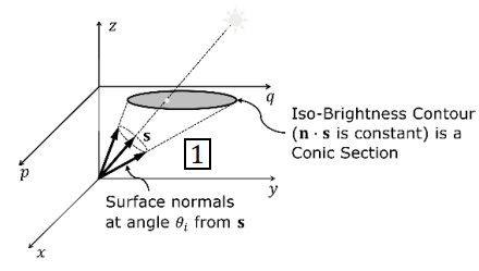
- Maximum Peak: When the surface normal points directly toward the light source ($p = p_s, q = q_s$), $\cos\theta_i = 1$, forming the brightest center of the map.
- Conic Sections: For Lambertian surfaces, normals sharing a constant angle with the light vector form a cone. The intersection of this cone with the $z=1$ gradient plane forms ellipses, parabolas, or hyperbolas in gradient space.
- Terminator (Shadow Line): At the boundary where brightness falls to zero ($I = 0$ or $90^\circ$ incident angle), setting the numerator to zero yields a straight line in gradient space:
$$p p_s + q q_s + 1 = 0$$
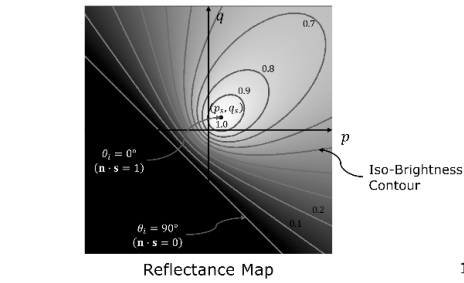
A single intensity measurement at a pixel restricts $(p,q)$ to one of these contours. Because infinitely many $(p,q)$ points lie along a single contour, recovering the surface normal from a single image is mathematically ambiguous.
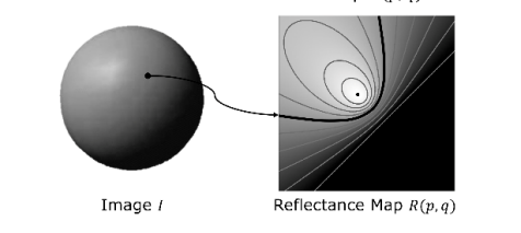
3. Resolving Ambiguity via Intersection in Photometric Stereo
Photometric Stereo resolves this infinite set of candidate orientations by intersecting iso-brightness contours obtained under controlled lights from different directions:
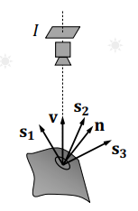
flowchart LR
subgraph Step1["1 Light Source (s1)"]
C1["R1(p,q) = I1 Contour"] --> Amb1["Infinite (p,q) Candidates"]
end
subgraph Step2["2 Light Sources (s1, s2)"]
C2["Intersection of R1 & R2 Contours"] --> Amb2["At most 2 Candidate Points"]
end
subgraph Step3["3 Light Sources (s1, s2, s3)"]
C3["Intersection of R1, R2 & R3 Contours"] --> Sol["Unique Single (p*, q*) Solution"]
end
Step1 --> Step2 --> Step3
style Amb1 fill:#393e46,stroke:#e94560,color:#fff
style Amb2 fill:#0f3460,stroke:#ffd369,color:#fff
style Sol fill:#1a1a2e,stroke:#4cc9f0,color:#fff
- One Light Source ($\mathbf{s}_1$): Measured intensity $I_1$ defines a contour $R_1(p,q) = I_1$. The true solution is one of infinitely many candidate points along this curve.
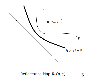
- Two Light Sources ($\mathbf{s}_1, \mathbf{s}_2$): A second light source yields intensity $I_2$ and contour $R_2(p,q) = I_2$. The two curves intersect at most at two points, reducing candidate normals to two.
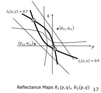
- Three Light Sources ($\mathbf{s}_1, \mathbf{s}_2, \mathbf{s}_3$): A third light source yields intensity $I_3$ and contour $R_3(p,q) = I_3$. Intersecting all three curves pinpoints a unique single $(p^, q^)$ point, completely resolving the surface normal ambiguity.
Key Insight: Each additional light source introduces an independent geometric constraint in gradient space. While two light sources reduce ambiguity to two points, a third light source uniquely resolves the true local surface normal.
4. Lambertian Case
When surface reflectance is ideal matte (Lambertian), surface normals can be computed rapidly using linear algebra without explicitly evaluating gradient space contours. Furthermore, spatially varying surface albedo ($\rho$) can be recovered simultaneously.
4.1 Linear System Formulation
Sequentially illuminating the scene with unit light sources $\mathbf{s}_1, \mathbf{s}_2, \mathbf{s}_3$ produces three measured pixel intensities according to Lambert’s law:
$$I_1 = \frac{\rho}{\pi} (\mathbf{n} \cdot \mathbf{s}_1), \quad I_2 = \frac{\rho}{\pi} (\mathbf{n} \cdot \mathbf{s}_2), \quad I_3 = \frac{\rho}{\pi} (\mathbf{n} \cdot \mathbf{s}_3)$$
We express this system as a compact matrix multiplication:
$$\mathbf{I} = S \mathbf{N}$$
Where:
- $\mathbf{I} = \begin{bmatrix} I_1 \ I_2 \ I_3 \end{bmatrix}$ is the $3 \times 1$ intensity vector.
- $S = \begin{bmatrix} \mathbf{s}1^T \ \mathbf{s}2^T \ \mathbf{s}3^T \end{bmatrix} = \begin{bmatrix} p{s1} & q{s1} & 1 \ p{s2} & q_{s2} & 1 \ p_{s3} & q_{s3} & 1 \end{bmatrix}$ is the known $3 \times 3$ light direction matrix.
- $\mathbf{N} = \frac{\rho}{\pi} \mathbf{n}$ is the albedo-scaled normal vector.
flowchart TD
Measurements["Intensity Vector I (3x1)"] --> Solver["Linear System Solver: N = S⁻¹ I"]
LightMatrix["Light Matrix S (3x3)"] --> Solver
Solver --> ScaledNormal["Scaled Normal Vector N"]
ScaledNormal --> Mag["Magnitude |N|"]
ScaledNormal --> Dir["Unit Vector N / |N|"]
Mag --> Albedo["Albedo (ρ = π |N|)"]
Dir --> SurfaceNormal["Unit Surface Normal (n)"]
style Solver fill:#1a1a2e,stroke:#4cc9f0,color:#fff
style ScaledNormal fill:#16213e,stroke:#ffd369,color:#fff
style Albedo fill:#0f3460,stroke:#e94560,color:#fff
style SurfaceNormal fill:#0f3460,stroke:#4cc9f0,color:#fff
If the light source vectors are linearly independent ($\det(S) \neq 0$), matrix $S$ is invertible, allowing direct computation of vector $\mathbf{N}$:
$$\mathbf{N} = S^{-1} \mathbf{I}$$
Decomposing magnitude and direction of $\mathbf{N}$ isolates albedo and unit surface normal simultaneously:
$$\text{Albedo } (\rho) = \pi |\mathbf{N}|$$
$$\text{Unit Surface Normal } (\mathbf{n}) = \frac{\mathbf{N}}{|\mathbf{N}|}$$
Example Reconstruction Results:
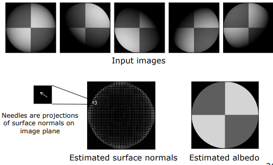
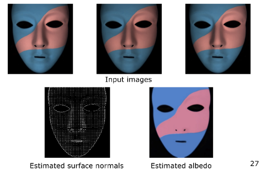
4.2 Singularities
If light vectors are coplanar, matrix $S$ becomes singular ($\det(S) = 0$), rendering the system unsolvable.
For example, when using sunlight variations throughout the day for outdoor photometric stereo, celestial geometry introduces singularities:
- Equinox Singularity: During an equinox, the sun moves along the celestial equator, causing all illumination vectors throughout the day to lie within the same plane ($\det(S) = 0$), making 3D recovery impossible.
4.3 Overdetermined Systems ($K > 3$) and Least Squares
To reduce noise sensitivity and eliminate shadow regions, $K$ ($K > 3$) light sources are often used, expanding $S$ to size $K \times 3$. The robust vector $\mathbf{N}$ is computed using Least Squares:
$$\mathbf{N} = (S^T S)^{-1} S^T \mathbf{I}$$
4.4 Effective Light Source Property
A crucial physical simplification applies specifically to Lambertian surfaces:
Multiple point lights or broad area light sources operating simultaneously (excluding cast shadows and interreflections) behave mathematically and physically as a single effective point light source ($\mathbf{s}_{\text{eff}}$) located at their intensity-weighted centroid.
Calibration-Based Photometric Stereo, Shape from Normals, and Interreflections
1. Calibration-Based Photometric Stereo
Many real-world materials (shiny plastics, varnished woods, metals) do not exhibit ideal matte Lambertian reflection; instead, they possess complex combinations of diffuse and specular reflections. Modeling the reflectance maps of such materials with analytical formulas is mathematically intractable.
To overcome this limitation, a data-driven approach called Calibration-Based Photometric Stereo is employed.
1.1 Orientation Consistency Principle
The core assumption of calibration-based photometric stereo is: If two distinct objects are fabricated from identical material and share the same surface normal (orientation) under identical light source conditions, they must produce identical pixel intensity combinations in the camera.
flowchart TD
subgraph Calib["1. Calibration Phase"]
Sphere["Calibration Sphere (Known Geometry)"] --> CaptureSphere["Acquire Images under K Lights"]
CaptureSphere --> Boundary["Occluding Boundary (r) & Analytical Normals (p,q)"]
Boundary --> LUT["Build Lookup Table (LUT)<br/>[I1, I2, ..., IK] ➔ (p, q)"]
end
subgraph Target["2. Target Object Phase"]
Object["Target Object (Same Material)"] --> CaptureObj["Acquire Images under Same K Lights"]
CaptureObj --> ReadPixel["Pixel Intensity Tuple [I1, ..., IK]"]
ReadPixel --> QueryLUT["Query Lookup Table (LUT)"]
LUT --> QueryLUT
QueryLUT --> Normals["Exact Surface Normals Map (p, q)"]
end
style Sphere fill:#1a1a2e,stroke:#4cc9f0,color:#fff
style LUT fill:#16213e,stroke:#ffd369,color:#fff
style Object fill:#0f3460,stroke:#e94560,color:#fff
style Normals fill:#1a1a2e,stroke:#4cc9f0,color:#fff
1.2 Implementation Steps
- Calibration Object: A calibration sphere coated with the exact same material as the target object and possessing known geometry is placed in the scene.
- Sphere Image Acquisition: The sphere is illuminated sequentially by $K$ light sources to acquire $K$ calibration images.
- Analytical Normal Map: By detecting the circular occluding boundary of the sphere, exact surface normals ($p, q$) for every sphere pixel are calculated analytically.
- Lookup Table (LUT) Construction: Measured intensity tuples $[I_1, I_2, \dots, I_K]$ serve as table keys, while known surface normals $[p, q]$ serve as table values.
- Target Object Estimation: The target object is illuminated under the same $K$ lights. For each pixel on the target, its measured intensity tuple is looked up in the LUT to retrieve its exact surface normal $[p, q]$.
This data-driven technique eliminates the need for analytical BRDF equations, yielding accurate surface normal maps for complex non-Lambertian industrial materials.
Key Insight: Calibration-based Photometric Stereo replaces complex analytical BRDF modeling with empirical mapping via a physical calibration sphere, enabling accurate reconstruction of shiny non-Lambertian surfaces.
2. Shape from Surface Normals
After applying Photometric Stereo, local surface gradient components ($p, q$) are obtained at every pixel. The objective of Shape from Surface Normals is to integrate these partial derivatives to reconstruct the 3D depth map ($z(x,y)$).
2.1 Naive Path Integration and Noise Breakdown
Theoretically, by setting a reference depth $z(x_0, y_0) = 0$ at the origin, depth at any pixel $(x,y)$ can be calculated by integrating gradients along a path:
$$z(x, y) = z(x_0, y_0) + \int_{x_0}^{x} -p , dx + \int_{y_0}^{y} -q , dy$$
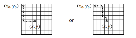
In real-world measurements, gradients contain noise. Under noisy gradients, path integration produces different depth values depending on the chosen path (e.g., integrating right-then-down vs down-then-right).
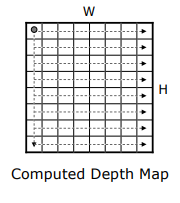
Errors accumulate progressively, leading to severe surface tearing and distortion.
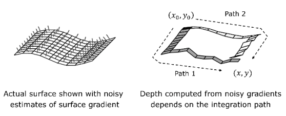
2.2 Frankot-Chellappa Integration Algorithm (Fourier Domain Least Squares)
To prevent noise accumulation, Frankot and Chellappa (1988) formulated a global Least Squares error functional that minimizes squared differences between partial derivatives of the target depth map $z(x,y)$ and measured gradients $p, q$ over the entire image:
$$D = \iint \left[ \left( \frac{\partial z}{\partial x} + p \right)^2 + \left( \frac{\partial z}{\partial y} + q \right)^2 \right] dx , dy$$
Solving this optimization in the Fourier domain transforms derivative operations into algebraic multiplications ($\mathcal{F}{\frac{\partial z}{\partial x}} = i u Z(u,v)$), yielding the optimal Fourier depth spectrum:
$$Z(u, v) = \frac{-i u P(u, v) - i v Q(u, v)}{u^2 + v^2}$$
flowchart TD
GradMap["Measured Gradients p(x,y) and q(x,y)"] --> FFT["2D Fast Fourier Transform (FFT)"]
FFT --> Spectra["Frequency Spectra P(u,v) and Q(u,v)"]
Spectra --> FrankotFormula["Frankot-Chellappa Formula:<br/>Z(u,v) = (-i u P - i v Q) / (u² + v²)"]
FrankotFormula --> DeepSpectrum["Optimal Depth Spectrum Z(u,v)"]
DeepSpectrum --> IFFT["Inverse 2D Fast Fourier Transform (IFFT)"]
IFFT --> GlobalDepth["Smooth 3D Depth Map z(x,y)"]
style FFT fill:#1a1a2e,stroke:#4cc9f0,color:#fff
style FrankotFormula fill:#16213e,stroke:#ffd369,color:#fff
style IFFT fill:#0f3460,stroke:#e94560,color:#fff
style GlobalDepth fill:#1a1a2e,stroke:#4cc9f0,color:#fff
Taking the Inverse Fast Fourier Transform (IFFT) of $Z(u,v)$ reconstructs a smooth, noise-resistant, globally consistent 3D depth map $z(x,y)$ in seconds.
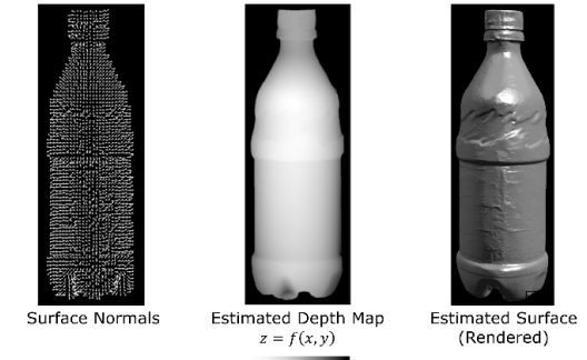
Key Insight: The Frankot-Chellappa algorithm replaces local path integration with a global optimization in the Fourier frequency domain, preventing local gradient noise from destroying surface continuity.
3. Interreflections
A fundamental assumption in standard photometric stereo is that scene points receive light exclusively from direct light sources. However, for concave geometries (such as bowls, cups, or deep grooves), secondary reflections break this assumption.
3.1 Destructive Effects of Interreflections
- Multiple Bounces: Inner surface points receive secondary and tertiary bounced rays reflected from neighboring concave patches in addition to direct light.
- Albedo Overestimation: Because secondary lighting increases observed brightness, calculated surface albedo ($\rho$) is severely overestimated.
- Surface Flattening (Shallower Depth): Additional light makes normal slope estimates steeper, causing depth integration to reconstruct concavities much shallower than their true depth.
3.2 Nayar-Ikeuchi-Kanade (1991) Iterative Algorithm
To remove interreflection artifacts, Nayar, Ikeuchi, and Kanade (1991) proposed an iterative radiosity-based algorithm:
flowchart TD
Step1["1. Standard Photometric Stereo & Frankot-Chellappa<br/>(Initial Flawed Shallow 3D Shape & Overestimated Albedo)"] --> Step2["2. Radiosity Simulation<br/>(Simulate secondary diffuse light contributions from current 3D geometry)"]
Step2 --> Step3["3. Image Compensation<br/>(Subtract simulated secondary rays from raw pixel intensities)"]
Step3 --> Step4["4. Re-run Photometric Stereo & Integration<br/>(Obtain deeper, more accurate 3D geometry)"]
Step4 --> Check{"Depth Convergence Reached?"}
Check -- "No" --> Step2
Check -- "Yes" --> Final["True Deep 3D Bowl Profile & True Albedo"]
style Step1 fill:#393e46,stroke:#e94560,color:#fff
style Step2 fill:#0f3460,stroke:#ffd369,color:#fff
style Step4 fill:#16213e,stroke:#4cc9f0,color:#fff
style Final fill:#1a1a2e,stroke:#4cc9f0,color:#fff
Iterative Steps:
- Initial Rough Estimation: Standard Photometric Stereo is run while ignoring interreflections, yielding an initial shallow shape and flawed albedo map.
- Interreflection Simulation: Using the estimated 3D geometry, secondary diffuse light contributions bouncing between surface points are simulated via radiosity equations.
- Image Compensation: Simulated secondary light components are subtracted from raw image intensities, creating interreflection-compensated images.
- Re-reconstruction: Photometric stereo and Frankot-Chellappa integration are re-run on compensated images to produce a deeper, more accurate 3D surface profile.
- Iteration & Convergence: The process repeats iteratively until the surface depth profile converges to the true deep concavity.
Key Insight: Interreflections cause concave surfaces to appear shallower than they are. The Nayar-Ikeuchi-Kanade algorithm iteratively simulates and subtracts bounced light components, converging to the exact deep 3D profile.
Shape from Shading
- 1. Overview and Core Classification
- 2. Human Perception of Shading
- 3. Stereographic Projection (f-g Space)
- 4. Shape from Shading Algorithm
- 5. Shading Illusions
- 6. Technical Summary Matrix
1. Overview and Core Classification
One of the most fundamental problems in computer vision, Shape from Shading (SfS), aims to recover the 3D surface geometry (surface normals or depth map) of objects in a scene from a single monochromatic (grayscale) image.
Key Insight: While Photometric Stereo requires multiple images taken under varying illumination sources, Shape from Shading attempts 3D reconstruction from a single image. This renders the problem physically and mathematically severely under-constrained.
flowchart TD
subgraph Input["Input"]
I["Single Grayscale Image I(x, y)"]
end
subgraph Problem["Mathematical Ambiguity"]
Iso["Iso-brightness Contour"]
Ambiguity["1 Equation vs 2 Unknowns (p, q) per Pixel"]
end
subgraph Solution["Strategies to Resolve Ambiguity"]
Phys["Physical Constraints (Smoothness & Boundary Conditions)"]
Priors["Psychophysical Priors (Light-from-Above, etc.)"]
end
I --> Iso --> Ambiguity
Ambiguity --> Phys
Ambiguity --> Priors
style Input fill:#1a1a2e,stroke:#4cc9f0,color:#fff
style Problem fill:#16213e,stroke:#e94560,color:#fff
style Solution fill:#0f3460,stroke:#4cc9f0,color:#fff
1.1 Mathematical Under-Constrained Problem
Assume we fully know the reflectance properties (BRDF) of a homogeneous material in the scene, as well as the light source direction ($\mathbf{s}$) and brightness. In this case, we can construct a Reflectance Map ($R(p, q)$) that gives the theoretical brightness at a camera pixel for any surface normal orientation (i.e., $p-q$ gradient).
However, reversing this physical process—inferring the surface normal orientation ($p, q$) at a point from a single measured pixel intensity ($I(x,y)$)—is mathematically impossible:
- Iso-Brightness Contour: In the reflectance map, points that equal the measured brightness ($I$) form a continuous curve called the iso-brightness contour.
- Infinite Candidate Normals: Infinite candidate surface normals ($p, q$ gradients) along this contour yield the exact same pixel intensity.
- Under-Constrained System: Having a single equation per pixel ($I(x,y) = R(p,q)$) with two independent unknown variables ($p$ and $q$) makes the problem severely under-constrained.
1.2 Strategy to Resolve Ambiguity
To overcome this infinite orientation ambiguity and reach a unique, stable geometric solution, two primary approaches are adopted:
- Physical / Mathematical Constraints: Assuming pixels cannot move independently, smoothness constraints and known boundary conditions are integrated into the scene.
- Psychophysical Priors: Analyzing how the human visual system resolves this ambiguity in milliseconds to formalize human visual heuristics into mathematical rules.
2. Human Perception of Shading
When viewing a single shaded photograph, the human visual system instantly perceives the object’s contours and 3D structure. The brain utilizes powerful prior assumptions about the physical world to resolve optical ambiguities.
flowchart LR
subgraph HumanPriors["Human Perception Priors"]
LFA["Light-from-Above Bias"]
SI["Sideways Illumination Ambiguity"]
GIC["Global Illumination Consistency"]
BOUND["Boundary Line Guidance"]
OVERRIDE["Prior Knowledge Override"]
end
style HumanPriors fill:#1a1a2e,stroke:#ffd369,color:#fff
style LFA fill:#0f3460,stroke:#4cc9f0,color:#fff
style SI fill:#0f3460,stroke:#4cc9f0,color:#fff
style GIC fill:#0f3460,stroke:#4cc9f0,color:#fff
style BOUND fill:#0f3460,stroke:#4cc9f0,color:#fff
style OVERRIDE fill:#0f3460,stroke:#e94560,color:#fff
2.1 Light from Above Bias
Derived from natural light sources (the sun and sky) always residing overhead, the human brain assumes light always emanates from top to bottom.
- Bumps vs. Concavities: If a circular shape on a panel is bright at the top and shaded at the bottom, the brain perceives it as convex (bump). If the bottom is bright and top shaded, it is interpreted as concave (hole).
- Mound vs. Crater Illusion: Rotating a photograph of a hill with a deep crater by $180^\circ$ causes the brain to perceive a massive crater with a central mound instead of just an inverted hill. The brain refuses to flip the light direction; instead, it reinterprets geometry to fit the “light from above” rule.
2.2 Sideways Illumination
When shading is oriented horizontally (light coming directly from left or right), the human visual system loses its default preference. Viewers become ambiguous between convex and concave interpretations. Shifting the mentally assumed light source flips the depth perception between bump and hollow.
2.3 Global Illumination Consistency
The human visual system assumes a single global light source illuminates all objects in a scene. If we perceive the top row of adjacent shapes as convex, we automatically interpret the lower row as concave to maintain lighting consistency.
2.4 Boundaries
Two strips sharing identical internal shading patterns can be perceived completely differently depending solely on their boundary cutout geometry:
- Sinusoidal Wavy Boundaries: Wavy boundary cutouts lead the brain to perceive internal shading as adjacent cylindrical waves (corrugated sheet).
- Sawtooth Boundaries: Triangular sawtooth boundaries transform identical shading into a folded corrugated roof perception. Boundary lines are the brain’s strongest geometric driver for shading interpretation.
2.5 Prior Knowledge Override
When encountering familiar structures, the human brain can override the “light from above” default rule:
- Hollow-Mask Illusion: Even when a concave human face mask is lit from above, the brain sees a convex protruding face because it knows human faces are convex. To preserve this prior depth perception, the brain accepts the illusion that lighting comes from below.
3. Stereographic Projection (f-g Space)
The conventional $(p, q)$ gradient space used to parameterize surface orientation suffers from severe numerical instability.
flowchart TD
subgraph Problems["p-q Gradient Space Limitation"]
PQ["p = -∂z/∂x, q = -∂z/∂y"]
Inf["p, q → ∞ as θ → 90° (Occluding Boundary)"]
Overflow["Numerical Overflow & Instability"]
end
subgraph Solution["f-g Stereographic Projection Solution"]
Sphere["Unit Sphere Surface Normal n"]
SouthPole["Projection from South Pole ([0, 0, -1]ᵀ)"]
Bounded["Maximum Bound: f² + g² ≤ 4 (Circle of Radius 2)"]
end
PQ --> Inf --> Overflow
Overflow -->|Stereographic Projection| Sphere --> SouthPole --> Bounded
style Problems fill:#1a1a2e,stroke:#e94560,color:#fff
style Solution fill:#0f3460,stroke:#4cc9f0,color:#fff
3.1 Limitations of p-q Gradient Space
Let unit surface normal $\mathbf{n}$ make an angle $\theta$ with the viewing direction ($z$-axis). Extending the normal to intersect the $z=1$ plane yields $p = -\partial z/\partial x$ and $q = -\partial z/\partial y$.
- As the surface steepens and the normal approaches grazing angle ($\theta \to 90^\circ$ occluding boundary), $p$ and $q$ grow boundlessly toward infinity ($\infty$).
- This leads to computational overflow errors, numerical instability, and non-linear resolution issues.
3.2 f-g Space (Stereographic Projection)
To resolve numerical bounds, the $f-g$ stereographic projection space is utilized:
- Projection originates from the South Pole ($[0, 0, -1]^T$) on the unit sphere.
- A straight ray from the South Pole passes through the unit normal vector ($\mathbf{n}$) and intersects the plane $z=1$ at $(f, g)$.
- Using similar triangles, the transformation between $(f,g)$ and $(p,q)$ is defined by:
$$f = \frac{2p}{1 + \sqrt{p^2 + q^2 + 1}}, \quad g = \frac{2q}{1 + \sqrt{p^2 + q^2 + 1}}$$
3.3 Numerical Advantage
Through this projection, all valid surface normals on the visible upper hemisphere map strictly inside a circle of radius 2 in $f-g$ space:
$$\text{Maximum Bound:} \quad f^2 + g^2 \leq 4$$
For instance, normal $(0, 1, 0)$ maps to $(0, 2)$, while $(1, 0, 0)$ maps to $(2, 0)$. Bounding values strictly within $[-2, 2]$ provides exceptional numerical stability for iterative SfS algorithms.
4. Shape from Shading Algorithm
Developed by Ikeuchi and Horn (1981), the numerical Shape from Shading algorithm combines three primary constraints to solve the ill-posed problem iteratively from boundary conditions inward.
flowchart TD
subgraph Constraints["Core Constraints & Boundary Conditions"]
BC["Boundary Condition (Occluding Boundary): n = e × v"]
IIC["Image Irradiance Constraint (e_R = ∬ (I - R_s)² dx dy)"]
SC["Smoothness Constraint (e_S = ∬ (||∇f||² + ||∇g||²) dx dy)"]
end
subgraph Optimization["Total Energy Minimization"]
Energy["e = e_S + λ e_R"]
Jacobi["Jacobi Iterative Scheme"]
end
subgraph Iteration["Iteration Loop"]
Init["Fix Boundaries, Initialize Internal Pixels to (0,0)"]
Avg["Compute 4-Neighbor Local Averages (f̄, ḡ)"]
Update["Update f^{(n+1)} and g^{(n+1)}"]
Conv{"Convergence Reached?"}
Depth["Frankot-Chellappa Integration to 3D Depth Map"]
end
BC --> Init
IIC --> Energy
SC --> Energy
Energy --> Jacobi --> Init
Init --> Avg --> Update --> Conv
Conv -- "No" --> Avg
Conv -- "Yes" --> Depth
style Constraints fill:#1a1a2e,stroke:#4cc9f0,color:#fff
style Optimization fill:#16213e,stroke:#ffd369,color:#fff
style Iteration fill:#0f3460,stroke:#4cc9f0,color:#fff
4.1 Boundary Condition Constraint (Occluding Boundaries)
The outer silhouette where an object curves out of sight is called the occluding boundary.
- At this boundary, the unit normal ($\mathbf{n}$) is perpendicular to both the viewing vector ($\mathbf{v}$) and the image boundary tangent vector ($\mathbf{e}$) ($\mathbf{n} \perp \mathbf{v}$ and $\mathbf{n} \perp \mathbf{e}$).
- Thus, boundary normals can be directly computed via the cross product:
$$\mathbf{n} = \mathbf{e} \times \mathbf{v}$$
These boundary normal values ($f, g$) serve as fixed Dirichlet Boundary Conditions, anchoring and propagating information into internal pixels.
4.2 Image Irradiance Constraint
Each computed $(f, g)$ orientation’s reflectance value ($R_s(f, g)$) must match the observed camera pixel intensity ($I(x,y)$). The error term ($e_R$) is formulated as:
$$e_R = \iint \left( I(x,y) - R_s(f, g) \right)^2 dx dy$$
4.3 Smoothness Constraint
To constrain the ill-posed problem, neighboring normals are assumed to change gradually (smooth surface). The squared partial derivatives of $f$ and $g$ ($e_S$) are minimized to penalize sharp orientation shifts:
$$e_S = \iint \left( \left(\frac{\partial f}{\partial x}\right)^2 + \left(\frac{\partial f}{\partial y}\right)^2 + \left(\frac{\partial g}{\partial x}\right)^2 + \left(\frac{\partial g}{\partial y}\right)^2 \right) dx dy$$
4.4 Total Energy Minimization & Iterative Solution (Jacobi Scheme)
Combining both error components via weighting factor $\lambda$ yields the total energy function ($e$):
$$e = e_S + \lambda e_R$$
Continuous derivatives are approximated via finite differences (Laplacian operator) on a 2D pixel grid. Taking partial derivatives with respect to each pixel ($f_{k,l}, g_{k,l}$) and setting them to zero derives the Jacobi iterative update scheme:
$$f_{k,l}^{(n+1)} = \bar{f}_{k,l}^{(n)} + \lambda \left( I_{k,l} - R_s(f_{k,l}^{(n)}, g_{k,l}^{(n)}) \right) \frac{\partial R_s}{\partial f}$$
$$g_{k,l}^{(n+1)} = \bar{g}_{k,l}^{(n)} + \lambda \left( I_{k,l} - R_s(f_{k,l}^{(n)}, g_{k,l}^{(n)}) \right) \frac{\partial R_s}{\partial g}$$
Where:
- $n$: Iteration step count.
- $\bar{f}_{k,l}^{(n)}$ and $\bar{g}_{k,l}^{(n)}$: Local averages of the 4 neighboring pixels (up, down, left, right). This term enforces geometric smoothness and boundary propagation.
- $\frac{\partial R_s}{\partial f}$ and $\frac{\partial R_s}{\partial g}$: Partial derivatives of the reflectance map based on the active BRDF model.
Holding boundary pixels fixed, internal pixels start at $[0, 0]^T$ and iterate until the difference between consecutive steps drops below a threshold. The output $(f, g)$ normal map is converted into a 3D depth surface via Fourier integration (Frankot-Chellappa).
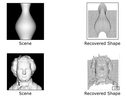
5. Shading Illusions
Both human visual perception and physical SfS principles trigger perceptual illusions because the human brain measures relative spatial gradients rather than absolute brightness.
5.1 Fading Disk Illusion
Focusing steadily without blinking at a fuzzy-bordered blue disk centered inside a large green circle causes the blue disk to gradually disappear into green.
- Physical Explanation: The human visual system is tuned to temporal and spatial variations (gradients) rather than absolute pixel intensity. Under fixed gaze (fixation), the smooth gradient boundary fails to trigger neural responses, leading the brain to fill in the region (filling-in process) with surrounding green color.
5.2 Checker Shadow Illusion
Created by Edward Adelson, this illusion places square “B” under a cylinder’s shadow and square “A” in open light. Square B appears dramatically lighter than A, yet masking surrounding context reveals both squares share identical physical grayscale pixel values.
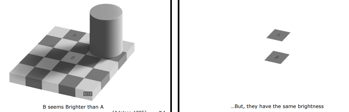
- Physical Explanation: The human visual system detects the gradual illumination drop caused by the shadow cast by the cylinder. To estimate true surface reflectance (albedo), the brain automatically filters out the illumination gradient. This intelligent illumination compensation leads the brain to perceive B as a lighter painted square despite identical raw pixel luminance values.
6. Technical Summary Matrix
| SfS Topic | Mathematical / Physical Constraint | Key Advantage | Failure Mode / Boundary |
|---|---|---|---|
| Mathematical Under-Constrained Problem | 1 intensity equation for 2 unknowns ($p, q$). | Defines theoretical limits of single-image 3D depth reconstruction. | Unsolvable without extra constraints (smoothness, boundary). |
| Human Perception of Shading | Light-from-above & single global light priors. | Provides strong geometric heuristics to resolve ambiguity. | Misinterpretations on familiar shapes (e.g. hollow-mask illusion). |
| Stereographic Projection | Homogeneous projection from South Pole to $z=1$ plane. | Bounds surface normals strictly within radius 2 disk ($[-2, 2]$). | Applicable only to visible upper hemisphere normals. |
| Ikeuchi-Horn Algorithm | Minimization of $e = e_S + \lambda e_R$ with Dirichlet boundary conditions. | Propagates boundary normals inward to reconstruct smooth 3D depth. | High error at sharp creases or non-smooth surface discontinuities. |
| Shading Illusions | Spatial gradient sensitivity & illumination filtering. | Reveals how the visual system filters and compensates for illumination. | Systematic errors when measuring absolute physical luminance. |
Depth from Focus & Defocus
- 1. Overview
- 2. Point Spread Function (PSF)
- 3. Depth from Focus (DFF)
- 4. Depth from Defocus (DFD)
- 5. Technical Comparison Summary
In computer vision, depth and shape recovery methods are generally divided into two main categories: active methods (laser scanners, structured light, etc.) and passive methods (stereo vision, shape from motion, etc.). Based on optical focus constraints, Depth from Focus (DFF) and Depth from Defocus (DFD) are passive and powerful depth sensing techniques that leverage the finite depth of field of single-lens cameras as a physical depth cue.
1. Overview
In images captured with a camera having a shallow depth of field, only objects located at the plane of focus appear sharp and crisp; objects in front of or behind this plane become defocused and blurred. According to optical physics, the amount and structure of blur are directly related to the physical distance of the object from the focus plane.
However, estimating local blur amount from a single image is mathematically an under-constrained problem. Given a single image patch, it is impossible to distinguish whether it appears blurry because it was captured out of focus or because the object’s original surface texture is inherently smooth/blurry. For example, a sharp photo of a smooth white wall looks identical locally to an out-of-focus photo of the same wall.
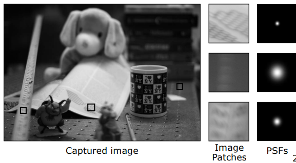
To overcome this ambiguity, multiple images taken under different focus settings or camera parameters are required. Two primary paradigms have been developed:
- Depth from Focus (DFF): Sweeps the focus plane step-by-step across the scene to collect a large focal stack. For each pixel coordinate, it searches for the image slice where contrast and sharpness are maximized.
- Depth from Defocus (DFD): Typically captures only two or three images with different focus or aperture settings. It calculates scene depth directly using analytical formulas or optimization techniques by analyzing relative blur ratios between the images.
2. Point Spread Function (PSF)
To mathematically model defocus blur, the spatial energy distribution formed on the sensor by an ideal point light source (impulse) must be defined. This distribution is called the Point Spread Function (PSF).
2.1 Circle of Confusion Geometry
According to the Gaussian Lens Law, a scene point at distance $u$ (or $o$) from a lens with focal length $f$ focuses perfectly at distance $v$ (or $i$) behind the lens:
$$\frac{1}{f} = \frac{1}{u} + \frac{1}{v}$$
If the sensor (image plane) is positioned at distance $s$ instead of the ideal focus distance $v$, focused rays intersect the sensor plane forming a circular light patch. Assuming a circular aperture, this base of the light cone is called the Blur Circle or Circle of Confusion.
Using similar triangles, the diameter of the blur circle ($b$) is related to aperture diameter ($D$) as follows:
$$\frac{b}{D} = \frac{|v - s|}{v} \implies b = D \cdot s \left| \frac{1}{s} - \frac{1}{v} \right|$$
This equation demonstrates two physical ways to control defocus blur amount:
- Vary Sensor Position ($s$): Translating the focal plane back and forth across the scene.
- Vary Aperture Size ($D$): Stopping down the lens (reducing $D$) narrows the light cone, shrinking blur diameter ($b$) and increasing depth of field.
2.2 Pillbox vs. Gaussian PSF Models
In an ideal, diffraction-free optical system, light distribution across the blur circle can be modeled as a uniform circular disk. This is termed the Pillbox Function:
$$h_{\text{pillbox}}(x, y) = \begin{cases} \frac{4}{\pi b^2}, & x^2 + y^2 \leq \frac{b^2}{4} \ 0, & \text{otherwise} \end{cases}$$
The normalization factor $\frac{4}{\pi b^2}$ enforces conservation of optical energy across expanding blur circles.
In real-world optical systems, diffraction at aperture edges, optical aberrations, surface roughness, and spatial pixel integration prevent sharp-edged pillbox distributions. Consequently, practical PSFs are realistically modeled as smooth Gaussian Functions:
$$h_{\text{Gaussian}}(x, y) = \frac{1}{2\pi \sigma^2} e^{-\frac{x^2+y^2}{2\sigma^2}}$$
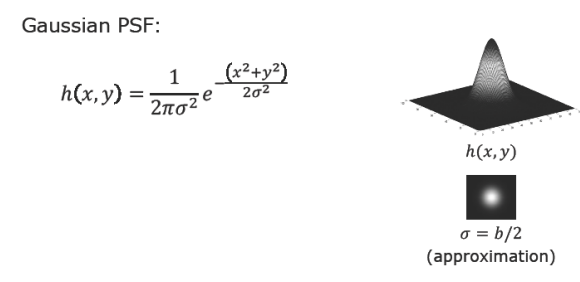
Empirically, Gaussian standard deviation ($\sigma$) relates to blur circle diameter ($b$) as:
$$\sigma \approx \frac{b}{2} \propto D \cdot s \left| \frac{1}{s} - \frac{1}{v} \right|$$
2.3 Convolution and Low-Pass Filter Equivalence
Assuming depth is locally constant over small patches, defocus imaging behaves as a Linear Shift-Invariant (LSI) system. Under LSI assumptions, the captured blurry image $g(x,y)$ equals the focused image $f(x,y)$ convolved with the PSF $h(x,y)$:
$$g(x, y) = f(x, y) * h(x, y)$$
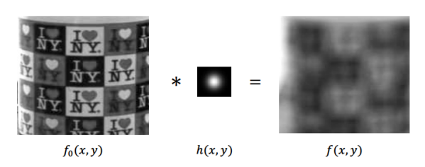
In the frequency (Fourier) domain, convolution converts to pointwise multiplication:
$$G(u, v) = F(u, v) \cdot H(u, v)$$
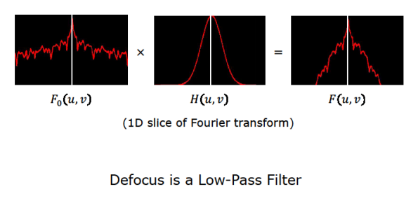
Because the Fourier transform of a Gaussian is also a Gaussian, an expanding PSF in spatial space ($\sigma$ growth) corresponds to a narrower Gaussian filter in frequency space.
Optically, defocus acts as a Low-Pass Filter. It preserves low-frequency macro structure while attenuating high-frequency textures, sharp edges, and fine details. Depth algorithms evaluate this high-frequency loss to infer distance.
3. Depth from Focus (DFF)
Depth from Focus (DFF) sweeps the focus plane across the scene in step increments to collect a focal stack, identifying the focal plane slice where high-frequency content peaks for each pixel.
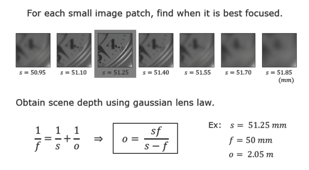
3.1 Focus Measure and Modified Laplacian
To evaluate sharpness across a focal stack, a local Focus Measure operator is defined. Since defocus suppresses high frequencies, local brightness variations (second derivatives) quantify sharpness.
In standard Laplacian operators, horizontal and vertical second derivatives can have opposite signs and cancel out. To prevent cancellation, the Modified Laplacian ($\nabla_M^2$) sums absolute partial second derivatives:
$$\nabla_M^2 I = \left| \frac{\partial^2 I}{\partial x^2} \right| + \left| \frac{\partial^2 I}{\partial y^2} \right|$$
On discrete pixel grids, partial derivatives are approximated by finite difference kernels:
$$\frac{\partial^2 I}{\partial x^2} = I(x+1, y) - 2I(x, y) + I(x-1, y)$$
$$\frac{\partial^2 I}{\partial y^2} = I(x, y+1) - 2I(x, y) + I(x, y-1)$$
The focus measure score $M(x,y)$ is computed by accumulating Modified Laplacian values within a local window (typically $3 \times 3$ or $5 \times 5$):
$$M(x, y) = \sum_{i=x-K}^{x+K} \sum_{j=y-K}^{y+K} \nabla_M^2 I(i, j)$$
3.2 Gaussian Interpolation for Smooth Reconstruction
Assigning depth directly to discrete focal stack layer indices causes depth resolution to be constrained by stack size $N$, creating staircase/contouring artifacts on 3D models. Increasing $N$ significantly increases capture time and memory footprint.
To achieve sub-stack precision, the focus measure distribution $M(s)$ near its peak is modeled as a Gaussian bell curve:
$$M(s) = M_p e^{-\frac{(s - \bar{s})^2}{2\sigma_m^2}}$$
Taking the natural logarithm linearizes the Gaussian model:
$$\ln M(s) = \ln M_p - \frac{(s - \bar{s})^2}{2\sigma_m^2}$$
Selecting the three highest discrete focus scores ($M_1, M_2, M_3$) and equal step size $\Delta s = s_2 - s_1 = s_3 - s_2$, an analytical closed-form solution yields continuous sensor location $\bar{s}$:
$$\bar{s} = s_2 + \frac{\Delta s \left( \ln M_3 - \ln M_1 \right)}{2 \left( 2 \ln M_2 - \ln M_1 - \ln M_3 \right)}$$
Substituting continuous $\bar{s}$ into the Gaussian lens law produces smooth, high-precision 3D depth maps.
DFF is extensively applied in microscopy and industrial quality inspection where shallow depth of field lens systems operate at micron scales.
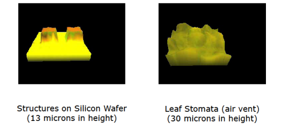
Key Limitation: DFF relies strictly on high-frequency surface texture; smooth, untextured regions cannot produce differential contrast variations across focus steps.
4. Depth from Defocus (DFD)
While DFF offers high accuracy, collecting tens of images is impractical for real-time video capture (30 FPS). Depth from Defocus (DFD) estimates depth rapidly by analyzing relative blur differences between as few as two images.
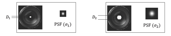
4.1 Naive DFD Solution (Ratio of Fourier Transforms)
Consider two images ($g_1, g_2$) of scene $f(x,y)$ taken with aperture sizes $D_1, D_2$ resulting in PSF widths $\sigma_1, \sigma_2$. Since aperture settings are hardware-controlled, the ratio of PSF widths is known:
$$\frac{\sigma_1}{\sigma_2} = \frac{D_1}{D_2} \implies \sigma_2 = \sigma_1 \frac{D_2}{D_1}$$
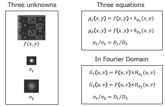
Writing spatial convolution equations in Fourier space:
$$G_1(u, v) = F(u, v) \cdot H_{\sigma_1}(u, v)$$
$$G_2(u, v) = F(u, v) \cdot H_{\sigma_2}(u, v)$$
Taking the ratio of Fourier transforms cancels the unknown true focused image $F(u,v)$:
$$\frac{G_1(u, v)}{G_2(u, v)} = \frac{H_{\sigma_1}(u, v)}{H_{\sigma_2}(u, v)}$$
Substituting Gaussian PSF formulas and taking logarithms yields an explicit expression for $\sigma_1$:
$$\sigma_1^2 - \sigma_2^2 = \frac{\ln G_2(u, v) - \ln G_1(u, v)}{2 \pi^2 (u^2 + v^2)}$$
Solving for $\sigma_1$ gives blur diameter $b_1 = 2\sigma_1$, from which scene depth $u$ is directly computed.
Warning: The naive Fourier ratio approach is unstable under sensor noise due to high-frequency division ($u^2+v^2$).
4.2 Reconstruction-Based Stable DFD
To handle noise robustly, Favaro (2003) and Pentland (1987) proposed an optimization-based formulation. The focused image $f$ and blur parameter $\sigma_1$ are estimated jointly by minimizing reconstruction error $E$:
$$E = \iint \left( g_1(x, y) - h_{\sigma_1} * f(x, y) \right)^2 dx dy + \iint \left( g_2(x, y) - h_{\sigma_1 \frac{D_2}{D_1}} * f(x, y) \right)^2 dx dy$$
Setting partial derivatives with respect to parameters to zero ($\frac{\partial E}{\partial \sigma_1} = 0, \frac{\partial E}{\partial f} = 0$) provides stable iterative solutions resilient to image noise.
4.3 Real-Time (Video-Rate) DFD System Architecture (Nayar 1996)
Nayar designed a dual-sensor optical setup utilizing a beam-splitter prism behind a single lens to split light onto two CCD sensors placed at different optical path lengths.
flowchart LR
Scene["Scene"] --> Lens["Single Lens"]
Lens --> BeamSplitter["Prism / Beam-Splitter"]
BeamSplitter --> CCD1["CCD1 (Near Focused Image)"]
BeamSplitter --> CCD2["CCD2 (Far Focused Image)"]
style Scene fill:#1a1a2e,stroke:#e94560,color:#fff
style Lens fill:#16213e,stroke:#0f3460,color:#fff
style BeamSplitter fill:#533483,stroke:#e94560,color:#fff
style CCD1 fill:#0f3460,stroke:#e94560,color:#fff
style CCD2 fill:#0f3460,stroke:#e94560,color:#fff
Simultaneous acquisition of near-focused and far-focused views enables real-time 3D depth map computation at 30 FPS.
4.4 Active Illumination for Textureless Surfaces
Since DFF and DFD rely on high-frequency surface detail, smooth textureless surfaces (such as uniform white walls) lack signal. Projecting a high-frequency artificial contrast pattern (active illumination mask) onto the scene provides synthetic texture, enabling real-time depth acquisition even on smooth or moving objects.
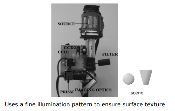
5. Technical Comparison Summary
| Feature / Method | Depth from Focus (DFF) | Depth from Defocus (DFD) |
|---|---|---|
| Number of Images | Large Focal Stack ($10 \sim 100$ images) | Minimal ($2 \sim 3$ images) |
| Mathematical Approach | Local Modified Laplacian ($\nabla_M^2$) & 3-point Gaussian Interpolation | Fourier PSF ratios or iterative reconstruction optimization |
| Depth Resolution | Extremely High (Microscopic precision) | Moderate-High (Ideal for video frame rates) |
| Computation Time | High (Processes full focal stack) | Low (Analyses relative difference between 2 images) |
| Texture Requirement | Essential (Fails on textureless regions) | Essential (Resolved via Active Illumination Pattern) |
| Hardware Setup | Motorized focal translation stage | Beam-splitter dual-sensor camera |
| Primary Applications | Microscopy, industrial quality control, medical imaging | Mobile cameras, consumer vision, real-time tracking |
Overview, Photometric Stereo Systems, and Structured Light Range Finding
In computer vision, cameras are traditionally passive observers that rely entirely on the ambient light available in the scene. However, in industrial automation, robotics, autonomous driving, and quality inspection, controlling illumination actively offers immense advantages. This strategic approach is known as Active Illumination.
1. Overview
Passive vision techniques (such as passive stereo vision and optical flow) rely on natural ambient lighting and surface appearance. Active illumination systems, by contrast, project controlled light energy onto the scene to reveal geometric and radiometric properties that are otherwise difficult or impossible to capture.
1.1 Limitations of Passive Vision and Advantages of Active Illumination
- Textureless Regions: Passive stereo vision and optical flow algorithms fail on homogeneous or featureless surfaces (e.g., a smooth white wall or uniform plastic housing) because robust correspondences cannot be found across camera views. Active illumination solves this by projecting artificial patterns (high-contrast structured light) onto the surface.
- Robustness to Ambient Lighting: In environments with fluctuating, unpredictable, or zero ambient illumination, active systems provide consistent, low-noise measurements using dedicated light sources.
- Photon Manipulation: By controlling the wavelength, direction, phase, and time-of-flight of emitted light, active vision systems extract hidden 3D geometric and material reflectance properties.
- Spectrum Selection (Human Invisibility): Active patterns can be projected in non-visible spectrums such as Infrared (IR) or Ultraviolet (UV). This allows high-precision 3D data acquisition without distracting humans (e.g., in smartphone facial authentication or night-time autonomous driving).
Key Insight: Active illumination converts ill-posed visual recovery problems into well-posed geometric or radiometric estimates by controlling the illumination field projected onto the scene.
2. Photometric Stereo Systems
Photometric stereo estimates surface normals by maintaining fixed camera and object positions while systematically varying the direction of illumination across multiple light sources.
2.1 Photometric Sampling
Traditional photometric stereo assumes that surface reflectance follows a purely Lambertian (diffuse) model. However, real-world objects display hybrid reflectance containing both diffuse and specular components. The Photometric Sampling theory proposed by Nayar (1989) addresses this limitation:
- Multi-LED Array: A large array of independently controlled LEDs is arranged on a spherical dome surrounding the object. These LEDs are sequentially triggered in sync with a high-speed camera within milliseconds.
- Diffuser Dome Integration: Point light sources cannot resolve pristine specular highlights on glossy or metallic surfaces because reflections appear only at isolated specular points. Placing a semi-transparent diffuser dome between the LED array and the object converts point sources into wide-angle area sources. This produces continuous, overlapping brightness fields, allowing precise extraction of surface normals even for complex metallic objects.
2.2 Debevec and “Light Stage” Technology
The principles of photometric sampling were scaled up by Paul Debevec and colleagues to capture human facial geometry and reflectance for film and computer graphics:
- High-Speed Scanning: A spherical cage equipped with hundreds of programmable LEDs (the “Light Stage”) rapidly cycles through varied lighting patterns at thousands of frames per second. Synchronized cameras capture the subject under dozens of distinct illumination angles in milliseconds.
- Relighting: The captured multi-illumination image sequence can be linearly combined to re-illuminate (relight) the subject under any target environment lighting. This process yields 3D surface geometry, pore-level micro-geometry, and separated diffuse and specular reflectance maps simultaneously.
3. Structured Light Range Finding
Structured light systems project known geometric light patterns onto a scene and compute direct depth ($z$) maps using optical triangulation.
flowchart TD
P["Projector (X_p, Y_p, Z_p)"] -->|"Light Ray / Plane"| S["Scene Point P(x, y, z)"]
C["Camera (X_c, Y_c, Z_c)"] -->|"Viewing Ray"| S
style P fill:#1a1a2e,stroke:#e94560,color:#fff
style C fill:#16213e,stroke:#4cc9f0,color:#fff
style S fill:#0f3460,stroke:#e94560,color:#fff
3.1 Point-Based Range Finding
- Operating Principle: A single laser pointer with precise position and orientation in projector space projects a narrow beam onto the scene, producing a bright spot $(x_i, y_i)$ on the camera sensor.
- Triangulation: The 3D line representing the camera viewing ray is intersected with the known 3D laser ray to compute the precise 3D coordinates $P(x, y, z)$ of the scene point.
- Background Subtraction: Images taken with and without the laser beam are subtracted to isolate the spot centroid with sub-pixel precision.
- Time Constraint: Since each image yields depth for only one point, capturing a $640 \times 480$ resolution depth map requires over 300,000 sequential images, making point scanning excessively slow for dynamic scenes.
3.2 Light Striping (Line-Based Range Finding)
Instead of a single point, a sheet of light (light plane) is generated using a cylindrical lens and projected onto the object, forming a curved stripe.
For each stripe pixel $(x_i, y_i)$ observed in the camera, depth $z$ is directly calculated by intersecting the camera ray with the known light plane equation $A x + B y + C z + D = 0$:
$$z = \frac{-D \cdot f}{A x_i + B y_i + C f}$$
where $f$ is the lens focal length.
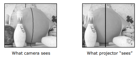
Sweeping the light plane across the scene with a motorized stage reduces the required frame count for a $640 \times 480$ depth map to just 640 images (~21 seconds at 30 fps).
3.3 Multi-Stripe Ambiguity
To achieve real-time speed, multiple stripes can be projected simultaneously in a single frame. However, this introduces correspondence ambiguity. On complex 3D surfaces with depth discontinuities or steep cavities, stripe order can swap or stripes can be occluded (shadowing). If the camera cannot uniquely match an observed stripe to its corresponding projector emission line, triangulation fails.
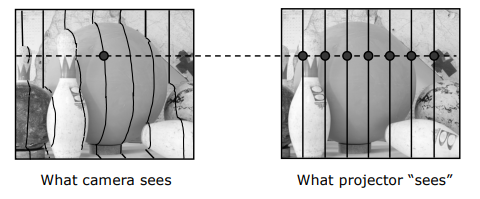
3.4 Binary Coded Structured Light
Space-time encoding resolves multi-stripe ambiguity by assigning a unique temporal binary codeword to each projection column:
- Codeword Logic: To encode 7 distinct stripes, $\log_2(7 + 1) = 3$ bits are required.
- Projection Pattern Sequence:
- Frame 1 (Bit 1): Stripes with first bit
1are illuminated; those with0remain dark (4 open, 3 dark). - Frame 2 (Bit 2): Stripes with second bit
1are illuminated. - Frame 3 (Bit 3): Stripes with third bit
1are illuminated.
- Frame 1 (Bit 1): Stripes with first bit
- A camera pixel observing the sequence
On-Off-Onacross the 3 frames decodes to binary $101_2 = 5$, establishing unambiguous matching to projector column 5.
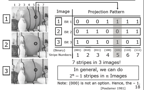
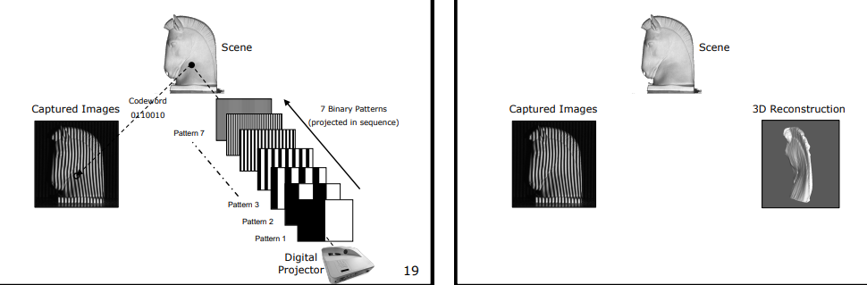
In general, $n$ sequential projection images can encode $2^n - 1$ distinct stripes (excluding 000 which represents total darkness). For instance, 8 images can uniquely encode 255 high-resolution stripes.
3.5 Light Bleeding and Gray Coding
- Light Bleeding Problem: Due to lens defocus and optical scattering, sharp black-white boundaries blur into continuous grayscale transitions. Thresholding boundary pixels into binary
0or1introduces severe depth estimation errors. Standard binary encoding has many simultaneous bit transitions between adjacent codes.
- Gray Code Solution (Inokuchi 1984): Gray coding ensures that adjacent stripes differ by only a single bit. Minimizing bit transitions dramatically reduces boundary thresholding errors caused by light bleeding.
3.6 Multi-Level and Color Coding (k-ary / Color Coded)
Instead of binary (on/off) coding, using $k$ intensity levels or distinct color channels (e.g., RGB ternary encoding where $k=3$) increases information density per frame:
- In a ternary system, encoding 7 stripes requires only 2 frames ($\log_3 8 \approx 2$), reducing the required frame count.
- In general, $n$ frames with $k$ levels encode $k^n - 1$ distinct stripes.
Limitations of Color Coding: Color crosstalk between camera/projector color channels and surface spectral absorption pose challenges. For instance, projecting a bright red stripe onto a deep blue object results in total light absorption, leaving zero backscatter for the camera. Color-coded structured light requires near-neutral diffuse reflectance (the gray world assumption) to operate reliably.
Phase Shifting Method, Structured Light Systems, and Time of Flight Method
While discrete binary patterns allow unambiguous triangulation, achieving sub-pixel 3D accuracy requires projecting continuous intensity functions across the scene. In this chapter, we explore continuous phase shifting, high-profile industrial structured light applications, fundamental optical limits, and Time-of-Flight (ToF) range sensing.
1. Phase Shifting Method
Rather than projecting discrete binary stripes, the phase shifting method projects mathematical light patterns whose intensities vary continuously across space. This increases spatial resolution to sub-pixel accuracy.
1.1 Intensity Ratio Method
- Ramp Function: A single ramp illumination pattern $L_1$ is projected onto the scene, where intensity decreases linearly from maximum brightness at one side to zero at the other ($x_p$).
- Flat Uniform Illumination: A second image is captured under flat uniform light $L_2$.
- Normalization: Measuring pixel intensities $I_1 = \rho \cdot L_1$ and $I_2 = \rho \cdot L_2$ in the camera and taking their ratio cancels the unknown surface albedo and surface normal factor $\rho$:
$$\frac{I_1}{I_2} = \frac{\rho \cdot L_1}{\rho \cdot L_2} = \frac{L_1}{L_2}$$
- Disadvantage: Highly sensitive to sensor noise and projector intensity quantization steps.
1.2 Sinusoidal Phase Shifting Mathematics
In industrial automation and quality inspection, the gold-standard technique is Sinusoidal Phase Shifting, which projects continuous cosine waves onto the scene and shifts their phase temporally.
The emitted projector cosine wave is defined by average brightness $b$, amplitude $b$, and period $P$. Accounting for unknown ambient lighting $a$ and relative surface albedo $\rho$, the pixel intensity observed by the camera is:
$$I_1(x_c, y_c) = \rho a + \rho b + \rho b \cos\left( \frac{2\pi x_p}{P} \right)$$
This equation contains three unknowns: $\rho a$ (ambient component), $\rho b$ (amplitude component), and the target projector column coordinate $x_p$. To solve for these three unknowns, exactly three phase-shifted images are captured:
- Frame 1 ($I_1$): Reference cosine pattern $L_1$ projected with $0^\circ$ phase shift.
- Frame 2 ($I_2$): Pattern phase shifted by $-120^\circ$ ($-2\pi/3$).
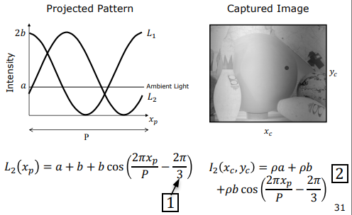
- Frame 3 ($I_3$): Pattern phase shifted by $+120^\circ$ ($+2\pi/3$).
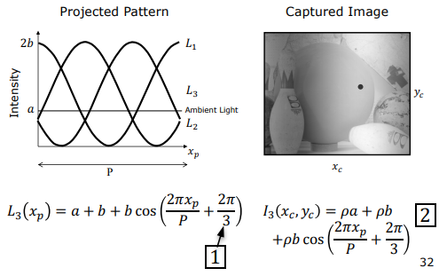
Solving these three simultaneous trigonometric equations eliminates ambient lighting $\rho a$ and amplitude $\rho b$, yielding a closed-form solution for projector column $x_p$:
$$x_p = \frac{P}{2\pi} \tan^{-1}\left( \sqrt{3} \frac{I_2 - I_3}{2I_1 - I_2 - I_3} \right)$$
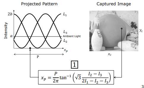
Intersecting the computed projector column plane $x_p$ with the camera viewing ray yields sub-millimeter 3D point accuracy.
2. Structured Light Systems
2.1 Notable High-Profile Systems
- 3D Visual Inspection (Omron Corp.): Used in surface-mount factory assembly lines to inspect printed circuit board (PCB) solder joints and micro-components in real time. The PCB is tiled and scanned via phase shifting in seconds to reject defective solder joints instantly.
- Digital Michelangelo Project (Levoy 2000): Stanford researchers scanned Michelangelo’s David statue in Florence over 30 nights using precision structured light range scanners. Achieving a mesh resolution of $1/4 \text{ mm}$, the project created a permanent digital twin (Virtual David) for micro-erosion tracking and archival preservation.
- Great Buddha Project (Ikeuchi 2007): Drone-mounted structured light and laser scanners were deployed in Nara, Japan to digitize the monumental Great Buddha statue and surrounding temple heritage structures.
2.2 Limitations and Unsolved Problems
Despite high accuracy, structured light systems face physical limitations on certain surface and material types:
- Specular / Metallic Surfaces: Mirror-like specular reflection redirects light exclusively along the angle of reflection. Light rarely backscatters to the camera, leaving empty holes in the depth map.
- Translucent / Subsurface Scattering Surfaces: On materials like marble, wax, or human skin, light penetrates beneath the surface and scatters internally before exiting from adjacent pixels, destroying pattern edge sharpness.
- Participating Media: In fog, smoke, or turbid underwater environments, light attenuates rapidly and ambient scattering causes the medium itself to glow, masking projected patterns.
- Transparent Objects (Glass/Water): Light refracts directly through glass objects without scattering.
- Hair and Micro-Fibers: Hair strands are far smaller than an individual camera pixel, causing multiple strands to project onto a single pixel and breaking geometric triangulation.
2.3 Summary of Structured Light Methods
The table below summarizes the image count complexity of all major structured light range finding paradigms:
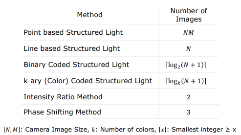
3. Time of Flight Method (ToF)
Time of Flight (ToF) range sensing bypasses baseline triangulation entirely by directly measuring the round-trip travel time of light ($c \approx 3 \times 10^8 \text{ m/s}$).
3.1 Biological Origins and Historical Speed of Light Experiments
- Biological Biosonar: Bats, dolphins, and whales use echolocation (sonar) by emitting sound waves and timing returning echoes to perceive 3D space. ToF applies this exact principle using light.
- Galileo’s Lantern Experiment (1600s): Galileo attempted to measure light speed by placing two lantern operators on hilltops 1000 meters apart (2000m round trip). Since light travels 2000m in just $6.6 \ \mu\text{s}$, human muscle reflexes (~milliseconds) rendered the experiment unsuccessful.
- Fizeau’s Cogwheel Experiment (1849): Hippolyte Fizeau successfully measured light speed by passing light through a rapidly spinning cogwheel over an $8633 \text{ m}$ distance to a plane mirror. By measuring the rotational speed at which returning light was blocked by adjacent teeth, he calculated $c_{\text{computed}} \approx 3.153 \times 10^8 \text{ m/s}$ (remarkably close to actual $2.998 \times 10^8 \text{ m/s}$).
3.2 Pulse Modulation (Flash ToF)
- Operating Principle: A short, high-power laser pulse is emitted into the scene. An ultra-fast nanosecond stopwatch measures the time delay $\Delta t$ before the reflected pulse strikes the sensor.
- Disadvantage: Sub-centimeter precision requires sub-nanosecond stopwatch electronics and high peak-power pulsed lasers, making high-resolution arrays costly.
3.3 Continuous Modulation (Phase ToF)
To avoid sub-nanosecond digital stopwatches, continuous modulation modulates emitted light intensity continuously using a high-frequency sinusoid (e.g., $f = 30 \text{ MHz}$).
Depth is directly proportional to the phase shift $\varphi$ measured between the emitted and returning cosine waves.
Correlation-Based Phase Measurement
The returning optical signal is demodulated by multiplying and integrating pixel charge against a reference signal $S_{ref}$ phase-locked to the emitter:
$$L_{emit} = \cos(\omega t)$$
$$L_{scene} = O + A \cos(\omega t - \varphi)$$
$$S_{ref} = \cos(\omega t - \delta)$$
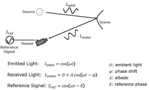
Measuring pixel charge under three distinct reference phase shifts ($\delta_1, \delta_2, \delta_3$) allows closed-form recovery of the unknown phase delay $\varphi$.
Phase-to-Distance Formula
Once phase shift $\varphi$ is recovered, absolute distance $d$ is given by:
$$d = c \frac{\varphi}{4\pi f}$$
Numerical Example: For modulation frequency $f = 30 \text{ MHz}$ and detected phase shift $\varphi = \pi$: $$d = (3 \times 10^8) \cdot \frac{\pi}{4\pi \cdot (30 \times 10^6)} = \frac{3 \times 10^8}{1.2 \times 10^8} = 2.5 \text{ meters}$$
3.4 Industrial Applications and Mobile Devices
- Autonomous Vehicles (LiDAR): Mechanical rotating LiDAR systems sweep single laser beams across $360^\circ$ to generate dense 3D point clouds for autonomous navigation. Solid-state LiDAR architectures are rapidly reducing cost and size.
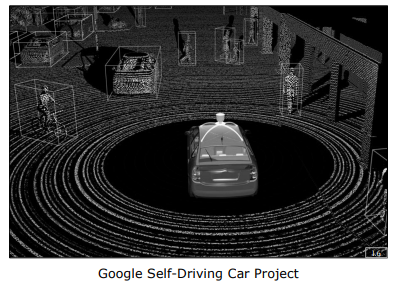
- Mobile Consumer Devices (Solid-State ToF): Modern smartphones and tablets integrate solid-state ToF sensor arrays. Instead of mechanical scanning, every pixel measures phase shift simultaneously, generating real-time depth maps for Augmented Reality (AR), portrait bokeh, and facial recognition.
Camera Models and Calibration
1. Overview
One of the fundamental goals of computer vision is to analyze 2D pixel coordinates in images to reconstruct the 3D metric structure of a scene. For a robot, autonomous vehicle, or augmented reality (AR) system to interact physically with the real world, scene dimensions must be converted from pixel units to physical units such as millimeters or meters.
The mathematical and optical process enabling this transition is called Camera Calibration. To define the imaging geometry of a camera and establish the mathematical bridge between 2D pixel coordinates and 3D world coordinates, two primary sets of parameters must be estimated:
- Extrinsic Parameters: Define the exact position (translation, $\mathbf{t}$) and orientation (rotation, $R$) of the camera relative to a 3D world coordinate system ($\mathcal{W}$).
- Intrinsic Parameters: Define the internal optical and hardware characteristics of the camera. This includes the lens focal length ($f$), pixel densities of the sensor ($m_x, m_y$), and the coordinates of the principal point ($o_x, o_y$) where the optical axis intersects the image plane.
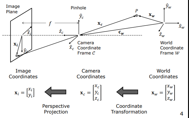
flowchart TD
subgraph Params["Camera Calibration Parameters"]
subgraph Extrinsic["Extrinsic Parameters"]
R["Rotation Matrix (R)<br/>3x3 Orthonormal Rotation"]
T["Translation Vector (t)<br/>3x1 Position Transformation"]
end
subgraph Intrinsic["Intrinsic Parameters"]
Focal["Focal Length (fx, fy)<br/>fx = mx*f, fy = my*f"]
PP["Principal Point (ox, oy)<br/>Sensor Optical Center"]
Skew["Skew Parameter (s)<br/>Pixel Shape Factor (typically 0)"]
end
end
Extrinsic --> WorldToCam["World to Camera Transformation (Mext)"]
Intrinsic --> CamToPixel["Camera to Pixel Transformation (Mint)"]
WorldToCam --> ProjMat["Projection Matrix P = Mint * Mext (3x4)"]
CamToPixel --> ProjMat
style Extrinsic fill:#0f3460,stroke:#e94560,color:#fff
style Intrinsic fill:#0f3460,stroke:#4cc9f0,color:#fff
style ProjMat fill:#1a1a2e,stroke:#e94560,color:#fff
Camera calibration numerically estimates these parameters using a calibration object with precisely known 3D geometry (such as a 3D checkerboard calibration cube). In this process, correspondences are established between known 3D world coordinates $\mathbf{X}{wi} = [x{wi}, y_{wi}, z_{wi}]^T$ on the calibration object and their corresponding 2D pixel projections $\mathbf{u}_i = [u_i, v_i]^T$ in the image.
Using these correspondences, a global $3 \times 4$ Projection Matrix ($P$) is solved first; then, this matrix is factored using linear algebra techniques (such as QR decomposition) to recover individual intrinsic and extrinsic parameters.
Key Insight: Without calibration, the physical size or distance of an object in an image cannot be known. Camera calibration is the bridge linking pixel counts to physical meters.
2. Linear Camera Model
The projection of a 3D point onto 2D pixel coordinates on the camera sensor is formalized in three steps by the Forward Imaging Model:
flowchart LR
World["3D World Point<br/>(Xw, Yw, Zw)"] -->|Extrinsic Transformation<br/>(R, t)| Cam["3D Camera Point<br/>(Xc, Yc, Zc)"]
Cam -->|Perspective Projection<br/>Lens Focal Length f| ImagePlane["2D Image Plane (mm)<br/>(xi, yi)"]
ImagePlane -->|Sensor Mapping<br/>Pixel Densities & Principal Point| Pixel["2D Pixel Coordinate<br/>(u, v)"]
style World fill:#1a1a2e,stroke:#e94560,color:#fff
style Cam fill:#16213e,stroke:#4cc9f0,color:#fff
style ImagePlane fill:#0f3460,stroke:#e94560,color:#fff
style Pixel fill:#0f3460,stroke:#4cc9f0,color:#fff
2.1 Perspective Projection (3D to 2D Millimeters)
In a pinhole camera model with the optical center (origin) located at $O_c$ and the optical axis aligned with $z_c$, the millimetric projection $(x_i, y_i)$ on the image plane of a scene point $(x_c, y_c, z_c)$ is derived using similar triangles:
$$\frac{x_i}{f} = \frac{x_c}{z_c} \implies x_i = f \frac{x_c}{z_c}$$
$$\frac{y_i}{f} = \frac{y_c}{z_c} \implies y_i = f \frac{y_c}{z_c}$$
where $f$ is the effective focal length of the camera in millimeters.
2.2 Sensor Mapping (Millimeters to Pixels)
A digital image sensor (CCD/CMOS) discretizes the continuous image plane into pixels. Sensor pixels may not be perfectly square; hence, horizontal pixel density $m_x$ (pixels/mm) and vertical pixel density $m_y$ (pixels/mm) are defined.
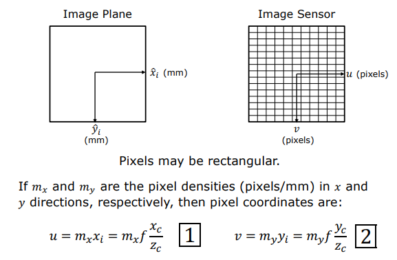
Furthermore, the Principal Point $(o_x, o_y)$, where the optical axis pierces the sensor, exhibits a pixel offset relative to the top-left origin $(0,0)$ of the image coordinate system.
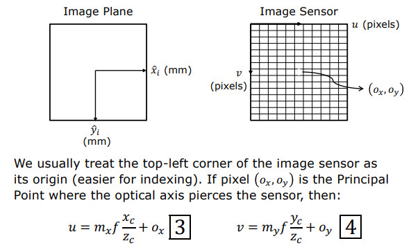
Combining these physical factors yields the digital pixel coordinates $(u, v)$:
$$u = m_x x_i + o_x = m_x f \frac{x_c}{z_c} + o_x$$
$$v = m_y y_i + o_y = m_y f \frac{y_c}{z_c} + o_y$$
To consolidate unknown hardware parameters, effective focal lengths in pixel units $f_x$ and $f_y$ are introduced:
$$f_x = m_x \cdot f \quad \text{and} \quad f_y = m_y \cdot f$$
This produces the non-linear projection equations:
$$u = f_x \frac{x_c}{z_c} + o_x \quad \text{and} \quad v = f_y \frac{y_c}{z_c} + o_y$$
2.3 Linearization via Homogeneous Coordinates
Due to the depth term $z_c$ in the denominator, the projection system is non-linear. To overcome this mathematical non-linearity, coordinates are mapped into Homogeneous Coordinate Space.
The 2D pixel coordinate $(u, v)$ is elevated to a homogeneous vector $[\tilde{u}, \tilde{v}, \tilde{w}]^T = [z_c u, z_c v, z_c]^T$. Geometrically, this mapping converts a 2D point into a 3D ray through the origin; intersecting this ray with the plane $\tilde{w}=1$ recovers Euclidean pixel coordinates.
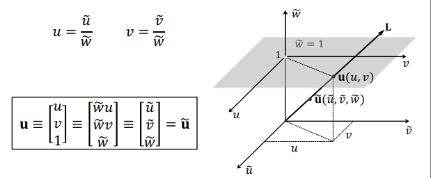
Similarly, the 3D scene point is represented as a 4D homogeneous vector $[x_c, y_c, z_c, 1]^T$:
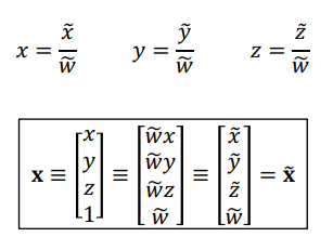
This elevation transforms perspective division into a linear matrix multiplication:

$$\begin{bmatrix} z_c u \ z_c v \ z_c \end{bmatrix} = \begin{bmatrix} f_x & 0 & o_x & 0 \ 0 & f_y & o_y & 0 \ 0 & 0 & 1 & 0 \end{bmatrix} \begin{bmatrix} x_c \ y_c \ z_c \ 1 \end{bmatrix}$$
3. Intrinsic and Extrinsic Matrices
The linear camera model is completely defined by two sub-matrices:
3.1 Intrinsic Matrix ($M_{int}$)
The intrinsic matrix represents the internal optical and hardware configuration of the camera as a $3 \times 4$ matrix:
$$M_{int} = \begin{bmatrix} K \mid \mathbf{0} \end{bmatrix} = \begin{bmatrix} f_x & 0 & o_x & 0 \ 0 & f_y & o_y & 0 \ 0 & 0 & 1 & 0 \end{bmatrix}$$
where $K$ is the $3 \times 3$ Calibration Matrix:
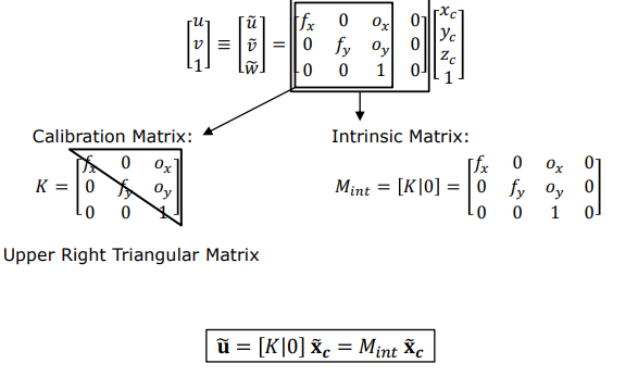
$$K = \begin{bmatrix} f_x & 0 & o_x \ 0 & f_y & o_y \ 0 & 0 & 1 \end{bmatrix}$$
Mathematical Note: The calibration matrix $K$ is an upper-right triangular matrix. If sensor pixels are non-perpendicular, a skew parameter $s$ can be placed at $K_{12} = s$; however, $s = 0$ for modern digital sensors.
3.2 Extrinsic Matrix ($M_{ext}$)
The extrinsic matrix maps a point $\mathbf{X}_w = [x_w, y_w, z_w]^T$ from the world coordinate frame ($\mathcal{W}$) into the camera frame ($\mathcal{C}$). Camera orientation is represented by a $3 \times 3$ Rotation Matrix ($R$), and camera position by a $3 \times 1$ Translation Vector ($\mathbf{t} = -R \mathbf{c}_w$):
$$\begin{bmatrix} x_c \ y_c \ z_c \ 1 \end{bmatrix} = M_{ext} \begin{bmatrix} x_w \ y_w \ z_w \ 1 \end{bmatrix} = \begin{bmatrix} R_{3 \times 3} & \mathbf{t}{3 \times 1} \ \mathbf{0}{1 \times 3} & 1 \end{bmatrix} \begin{bmatrix} x_w \ y_w \ z_w \ 1 \end{bmatrix}$$
The rotation matrix $R$ is orthonormal, satisfying $R^T R = I$ and $\det(R) = +1$.
3.3 Projection Matrix ($P$)
Multiplying the intrinsic and extrinsic matrices sequentially yields the $3 \times 4$ Projection Matrix ($P$), which directly maps 3D world coordinates to 2D pixel coordinates:
$$\tilde{\mathbf{u}} = M_{int} \cdot M_{ext} \cdot \tilde{\mathbf{X}}_w = P \cdot \tilde{\mathbf{X}}_w$$
$$P = K \begin{bmatrix} R \mid \mathbf{t} \end{bmatrix} = \begin{bmatrix} p_{11} & p_{12} & p_{13} & p_{14} \ p_{21} & p_{22} & p_{23} & p_{24} \ p_{31} & p_{32} & p_{33} & p_{34} \end{bmatrix}$$
flowchart TD
WorldPt["3D World Coordinate (Xw, Yw, Zw, 1)^T"] -->|Extrinsic Matrix Mext (4x4)| CamPt["3D Camera Coordinate (Xc, Yc, Zc, 1)^T"]
CamPt -->|Intrinsic Matrix Mint (3x4)| HomogPixel["Homogeneous Pixel Vector (z_c*u, z_c*v, z_c)^T"]
WorldPt -->|Direct Projection Matrix P (3x4)| HomogPixel
HomogPixel -->|Scale Normalization (Euclidean Homogenization)| PixelCoord["2D Pixel Coordinate (u, v)"]
style WorldPt fill:#0f3460,stroke:#e94560,color:#fff
style CamPt fill:#0f3460,stroke:#4cc9f0,color:#fff
style HomogPixel fill:#1a1a2e,stroke:#e94560,color:#fff
style PixelCoord fill:#16213e,stroke:#4cc9f0,color:#fff
4. Camera Calibration
The objective of camera calibration is to determine the 12 unknown parameters ($p_{11}$ through $p_{34}$) of the projection matrix $P$ by solving a linear system.
flowchart TD
Step1["1. Data Acquisition:<br/>Known 3D cube coordinates (Xwi, Ywi, Zwi)<br/>and corresponding 2D pixel points (ui, vi)"] --> Step2["2. DLT Linear System Assembly:<br/>2 equations per point -> A*p = 0<br/>(A matrix of dimension 2n x 12)"]
Step2 --> Step3["3. Constrained Least Squares Solution:<br/>min ||A*p||^2 s.t. ||p||^2 = 1<br/>SVD right singular vector (p) for smallest singular value"]
Step3 --> Step4["4. Matrix Factorization (Decomposition):<br/>Partition P = [B | p4].<br/>Perform QR (RQ) decomposition on B = K*R."]
Step4 --> Step5["5. Parameter Extraction:<br/>Intrinsic K, Rotation R,<br/>Translation t = K^(-1)*p4"]
style Step1 fill:#0f3460,stroke:#4cc9f0,color:#fff
style Step2 fill:#0f3460,stroke:#4cc9f0,color:#fff
style Step3 fill:#1a1a2e,stroke:#e94560,color:#fff
style Step4 fill:#0f3460,stroke:#4cc9f0,color:#fff
style Step5 fill:#16213e,stroke:#4cc9f0,color:#fff
4.1 Direct Linear Transformation (DLT)
For $i = 1, \dots, n$ points on a calibration object, known 3D world coordinates $(x_{wi}, y_{wi}, z_{wi})$ are paired with measured 2D pixel coordinates $(u_i, v_i)$.
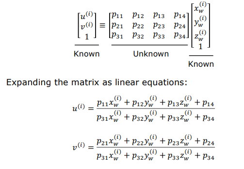
Expanding the homogeneous projection equation:
$$\begin{bmatrix} z_{ci} u_i \ z_{ci} v_i \ z_{ci} \end{bmatrix} = \begin{bmatrix} p_{11} & p_{12} & p_{13} & p_{14} \ p_{21} & p_{22} & p_{23} & p_{24} \ p_{31} & p_{32} & p_{33} & p_{34} \end{bmatrix} \begin{bmatrix} x_{wi} \ y_{wi} \ z_{wi} \ 1 \end{bmatrix}$$
Expressing depth from line 3 as $z_{ci} = p_{31} x_{wi} + p_{32} y_{wi} + p_{33} z_{wi} + p_{34}$ and substituting into lines 1 and 2 eliminates $z_{ci}$, yielding two independent linear equations per 3D-2D point pair:
$$(p_{11} x_{wi} + p_{12} y_{wi} + p_{13} z_{wi} + p_{14}) - u_i (p_{31} x_{wi} + p_{32} y_{wi} + p_{33} z_{wi} + p_{34}) = 0$$
$$(p_{21} x_{wi} + p_{22} y_{wi} + p_{23} z_{wi} + p_{24}) - v_i (p_{31} x_{wi} + p_{32} y_{wi} + p_{33} z_{wi} + p_{34}) = 0$$
Stacking these equations for all $n$ calibration points ($n \ge 6$) forms a $2n \times 12$ matrix $A$ and a 12-element parameter vector $\mathbf{p} = [p_{11}, p_{12}, \dots, p_{34}]^T$:
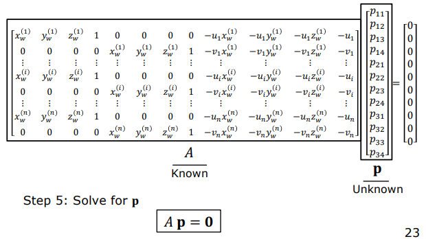
$$A \mathbf{p} = \mathbf{0}$$
4.2 Constrained Least Squares Solution
Because homogeneous coordinates operate up to an arbitrary scale factor ($\lambda P$ projects to the same pixels as $P$), a unit norm constraint $|\mathbf{p}|^2 = 1$ is enforced to resolve scale ambiguity.
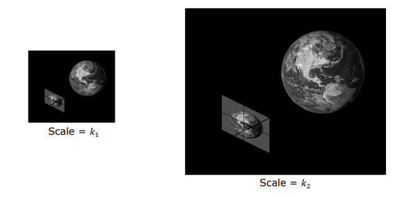
To minimize measurement noise, the constrained optimization problem is formulated:
$$\min_{\mathbf{p}} |A \mathbf{p}|^2 \quad \text{subject to} \quad |\mathbf{p}|^2 = 1$$
Theoretical Proof (Lagrange Multipliers)
Formulating the Lagrangian with multiplier $\lambda$:
$$\mathcal{L}(\mathbf{p}, \lambda) = \mathbf{p}^T A^T A \mathbf{p} - \lambda (\mathbf{p}^T \mathbf{p} - 1)$$
Taking the partial derivative with respect to $\mathbf{p}$ and setting it to zero:
$$\frac{\partial \mathcal{L}}{\partial \mathbf{p}} = 2 A^T A \mathbf{p} - 2 \lambda \mathbf{p} = \mathbf{0} \implies A^T A \mathbf{p} = \lambda \mathbf{p}$$
This is the standard Eigenvalue / Eigenvector Problem.
Substituting back into the objective function $|A \mathbf{p}|^2$:
$$|A \mathbf{p}|^2 = \mathbf{p}^T A^T A \mathbf{p} = \mathbf{p}^T (\lambda \mathbf{p}) = \lambda \mathbf{p}^T \mathbf{p} = \lambda$$
Proof Conclusion: Minimizing $|A \mathbf{p}|^2$ corresponds to selecting the smallest eigenvalue $\lambda_{\min}$ of $A^T A$. Thus, the optimal parameter vector $\mathbf{p}$ is the eigenvector associated with the smallest eigenvalue of $A^T A$ (or equivalently, the right singular vector $V_{*,12}$ corresponding to the smallest singular value in the Singular Value Decomposition $A = U \Sigma V^T$).
Reshaping the optimal vector $\mathbf{p}$ into a $3 \times 4$ grid reconstructs the Projection Matrix $P$.
4.3 Decomposing the Projection Matrix
To extract explicit intrinsic ($K$) and extrinsic ($R, \mathbf{t}$) parameters from $P$:
- Separating Calibration ($K$) and Rotation ($R$): Let $B$ denote the leading $3 \times 3$ submatrix of $P$: $$P = [B_{3 \times 3} \mid \mathbf{p}_4] = [K \cdot R \mid K \cdot \mathbf{t}]$$ Since $K$ is upper-triangular and $R$ is orthonormal ($R R^T = I$), QR Decomposition (or RQ factorization) uniquely factors $B = K \cdot R$ into $K$ and $R$.
- Solving the Translation Vector ($\mathbf{t}$): The last column $\mathbf{p}_4$ of $P$ satisfies $\mathbf{p}_4 = K \mathbf{t}$. Inverting $K$ yields the translation vector: $$\mathbf{t} = K^{-1} \mathbf{p}_4$$
4.4 Optical Lens Distortions
Real lens systems exhibit non-linear departures from the ideal pinhole model. While projection matrix $P$ models linear perspective geometry, non-linear lens aberrations are modeled separately and corrected after linear calibration:
- Radial Distortion: Caused by light rays refracting differently near the edges of spherical lenses (Barrel or Pincushion distortion).
- Tangential Distortion: Caused by slight physical misalignment of lens elements relative to the image sensor plane.
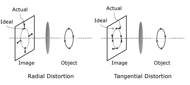
This completes the full recovery of camera intrinsics ($K$), extrinsics ($R, \mathbf{t}$), and optical distortion parameters.
Simple Stereo Vision and Depth
- 1. Backward Projection Ambiguity
- 2. Simple Stereo Geometry
- 3. Disparity & Depth Relationship
- 4. Stereo Matching Challenges
1. Backward Projection Ambiguity
Even when a single camera is fully calibrated with known intrinsic ($K$) and extrinsic ($R, \mathbf{t}$) parameters, a single 2D image alone is insufficient to reconstruct the 3D depth of a scene.
Consider a calibrated camera observing a 2D pixel coordinate $(u, v)$ on the image plane. Attempting to recover its unique 3D Euclidean coordinates $(x, y, z)$ encounters a fundamental mathematical limitation.
flowchart LR
Pixel["2B Pixel (u, v)"] -->|Backward Projection| Ray["3D Outgoing Ray<br/>x = z/fx * (u - ox)<br/>y = z/fy * (v - oy)"]
Ray -->|Unknown Depth z| Ambiguity["Ambiguity:<br/>Scene point can lie at any<br/>depth z along this ray!"]
style Pixel fill:#0f3460,stroke:#4cc9f0,color:#fff
style Ray fill:#1a1a2e,stroke:#e94560,color:#fff
style Ambiguity fill:#16213e,stroke:#4cc9f0,color:#fff
The pixel $(u,v)$ specifies an outgoing 3D ray originating from the optical center $(0,0,0)$ and passing through the cell center on the image plane:
$$\text{2D-to-3D Backward Ray:} \quad x = \frac{z}{f_x} (u - o_x), \quad y = \frac{z}{f_y} (v - o_y), \quad z > 0$$
The physical scene point could lie at any depth $z$ along this ray. Thus, recovering depth from a single image is mathematically ill-posed; this is known as Backward Projection Ambiguity.
To resolve depth unambiguously, a second camera viewing the scene from a different viewpoint is required to intersect this ray via triangulation.
Key Insight: This is why biological vision systems employ two eyes. A single eye provides depth cues through shading and perspective, but binocular vision enables precise 3D depth computation through optical triangulation.
2. Simple Stereo Geometry
A Simple Stereo System consists of two identical cameras placed with parallel optical axes, identical vertical alignment, and separated horizontally by a distance $b$. The horizontal distance $b$ between the optical centers is called the Baseline.
flowchart TD
subgraph StereoRig["Simple Stereo Rig (Baseline = b)"]
LeftCam["Left Camera Center (0, 0, 0)<br/>Left Projection: (ul, vl)"]
RightCam["Right Camera Center (b, 0, 0)<br/>Right Projection: (ur, vr)"]
end
LeftCam -->|Left Ray| ScenePt["3D Scene Point (x, y, z)<br/>Intersection Point"]
RightCam -->|Right Ray| ScenePt
style LeftCam fill:#0f3460,stroke:#4cc9f0,color:#fff
style RightCam fill:#0f3460,stroke:#4cc9f0,color:#fff
style ScenePt fill:#1a1a2e,stroke:#e94560,color:#fff
In physical hardware, simple stereo systems are built by mounting two identical sensors in a single housing separated by a fixed baseline:
Scan-line Correspondence Constraint
Because the cameras differ only by a horizontal shift ($b$ along the $x$-axis), vertical pixel coordinates are identical in both views:
$$v_l = v_r$$
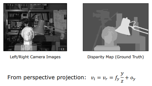
This geometric constraint eliminates the need to search the entire 2D image plane for matching pixels. The corresponding pixel in the right image must lie on the exact same horizontal scanline.
Algorithmic Advantage: Reducing the search space from 2D to 1D drops matching complexity from $O(N^2)$ to $O(N)$, dramatically boosting efficiency and matching accuracy.
3. Disparity & Depth Relationship
The perspective projection equations for a 3D point $(x, y, z)$ onto the left and right cameras are:
$$\text{Left Camera:} \quad u_l = f_x \frac{x}{z} + o_x \quad \text{and} \quad v_l = f_y \frac{y}{z} + o_y$$
$$\text{Right Camera:} \quad u_r = f_x \frac{x - b}{z} + o_x \quad \text{and} \quad v_r = f_y \frac{y}{z} + o_y$$
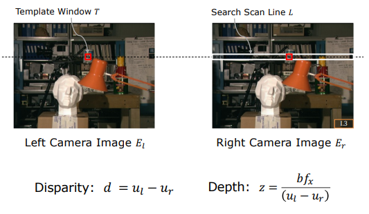
The horizontal pixel shift between corresponding points is defined as Disparity ($d$):
$$d = u_l - u_r$$
Substituting projection equations into the disparity expression yields:
$$d = \left(f_x \frac{x}{z} + o_x\right) - \left(f_x \frac{x - b}{z} + o_x\right) = f_x \frac{b}{z}$$
Triangulating depth and 3D point coordinates from disparity:
$$z = \frac{f_x \cdot b}{u_l - u_r} = \frac{f_x \cdot b}{d}$$
$$x = \frac{b (u_l - o_x)}{u_l - u_r}$$
$$y = \frac{b f_x (v_l - o_y)}{f_y (u_l - u_r)}$$
Key Physical Principles
- Inverse Relationship ($z \propto 1/d$): Depth is inversely proportional to disparity. Nearby objects undergo large pixel shifts (large disparity). As distance increases, disparity shrinks. At infinity ($z \to \infty$), disparity approaches zero ($d \to 0$).
- Baseline Scaling ($d \propto b$): Increasing the baseline $b$ expands disparity across a wider pixel range. For long-range sensing, a wider baseline is essential to maintain depth resolution over discrete pixels.
4. Stereo Matching Challenges
Computing depth via triangulation requires finding corresponding pixels between left and right images. This process is called Stereo Matching (The Correspondence Problem).
4.1 Similarity Metrics: SAD, SSD, and NCC
To match pixels along the horizontal scanline, a template window ($W$) is shifted across the candidate search line:
- SAD (Sum of Absolute Differences): Computes the sum of absolute intensity differences. Computationally fastest: $$\text{SAD}(u, v, d) = \sum_{(x,y) \in W} |I_l(u+x, v+y) - I_r(u+x-d, v+y)|$$
- SSD (Sum of Squared Differences): Penalizes larger intensity discrepancies more heavily: $$\text{SSD}(u, v, d) = \sum_{(x,y) \in W} (I_l(u+x, v+y) - I_r(u+x-d, v+y))^2$$
- NCC (Normalized Cross-Correlation): Normalizes window intensities by mean and variance. Highly robust against lighting changes and exposure shifts: $$\text{NCC}(u, v, d) = \frac{\sum (I_l - \bar{I}_l)(I_r - \bar{I}_r)}{\sqrt{\sum (I_l - \bar{I}_l)^2 \sum (I_r - \bar{I}_r)^2}}$$
4.2 Window Size Trade-off
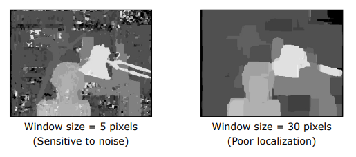
- Small Windows (e.g., $3 \times 3$ or $5 \times 5$): Provide sharp boundary localization but are sensitive to image noise and spurious matches.
- Large Windows (e.g., $21 \times 21$ or $31 \times 31$): Smooth out image noise but blur sharp depth transitions and object boundaries.
4.3 Physical Limitations of Stereo Vision
Three main physical scenarios degrade stereo matching performance:
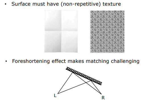
- Textureless Surfaces: Uniform surfaces (e.g., blank walls) yield flat similarity scores across the scanline, rendering pixel matching ambiguous.
- Repetitive Patterns: Periodic structures (e.g., fences or checkerboards) produce multiple strong correlation peaks, causing matching ambiguity.
- Foreshortening: Slanted surfaces viewed from different angles undergo non-uniform pixel compression, degrading window correlation.
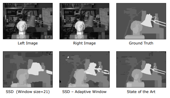
Modern approaches overcome local window limitations using Adaptive Windows, Global Optimization (Graph Cuts, Belief Propagation), and Deep Learning Stereo Architectures (Stereo CNNs).
Uncalibrated Stereo Vision and Epipolar Geometry
- 1. Overview
- 2. Problem of Uncalibrated Stereo
- 3. Epipolar Geometry
- 4. Estimating Fundamental Matrix
- 5. Finding Correspondences
- 6. Computing Depth
- 7. Stereo Vision in Nature (Stereopsis)
- 8. Summary Technical Comparison Matrix
One of the most exciting and powerful domains of computer vision is reconstructing the three-dimensional (3D) geometry of a scene from scratch without prior knowledge of camera positions or orientations ($R, \mathbf{t}$). By leveraging pixel correspondences across multiple uncalibrated images alongside intrinsic optical parameters, 3D structure can be estimated robustly. This note provides an in-depth treatment of Epipolar Geometry, Essential Matrix ($E$), Fundamental Matrix ($F$) estimation via the 8-point algorithm, 1D Epipolar Search for dense correspondence, Linear Triangulation, and the physiological/psychophysical mechanisms of Stereo Vision in Nature (Stereopsis) based on the Columbia CAVE curriculum (Prof. Shree K. Nayar).
1. Overview
In calibrated (simple) stereo systems, the cameras are fixed, their optical axes are strictly parallel, their vertical rows are aligned, and the horizontal baseline distance ($b$) between them is known with millimeter precision.
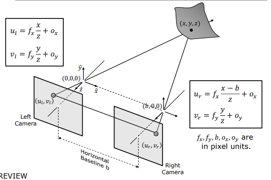
In a simple stereo rig where the left camera is at $(0,0,0)$ and the right camera is displaced at $(b,0,0)$, 3D coordinates $(x,y,z)$ are recovered directly from pixel coordinates $(u_l, v_l), (u_r, v_r)$ and horizontal disparity ($d = u_l - u_r$):
$$x = \frac{b(u_l - o_x)}{u_l - u_r}, \quad y = \frac{b \cdot f_x (v_l - o_y)}{f_y (u_l - u_r)}, \quad z = \frac{b \cdot f_x}{u_l - u_r}$$
However, in real-world scenarios—such as crowd-sourced tourist photos or handheld mobile captures—the relative 3D positions and rotation angles of the cameras are completely unknown.
Uncalibrated Stereo enables 3D scene reconstruction from two or more arbitrary images without pre-measuring relative camera translation ($\mathbf{t}$) or rotation ($R$).
flowchart LR
subgraph CalibratedStereo["Calibrated Stereo (Simple Stereo)"]
direction TB
C1["Fixed Baseline (b)"] --> C2["Parallel Optical Axes"]
C2 --> C3["Horizontally Aligned Epipolar Lines (d = ul - ur)"]
end
subgraph UncalibratedStereo["Uncalibrated Stereo"]
direction TB
U1["Unknown Rotation (R) & Translation (t)"] --> U2["Angled / Arbitrary Epipolar Lines"]
U2 --> U3["Fundamental Matrix (F) & Essential Matrix (E)"]
end
style CalibratedStereo fill:#0f3460,stroke:#4cc9f0,color:#fff
style UncalibratedStereo fill:#1a1a2e,stroke:#e94560,color:#fff
Assuming camera intrinsic calibration matrices ($K_l, K_r$) can be obtained (e.g., from EXIF metadata), the uncalibrated stereo pipeline analyzes geometric epipolar constraints to recover relative pose parameters ($R, \mathbf{t}$) and compute dense scene depth simultaneously.
Key Insight: Uncalibrated stereo forms the foundational mathematical engine of modern Structure from Motion (SfM) and Photo Tourism pipelines. Even with zero prior pose information, 3D world coordinates are successfully recovered strictly from pixel feature matches.
2. Problem of Uncalibrated Stereo
The core objective of uncalibrated stereo is recovering 3D scene structure from two uncalibrated views with an unknown spatial relationship ($R, \mathbf{t}$).
The problem is resolved through a systematic 5-step processing pipeline:
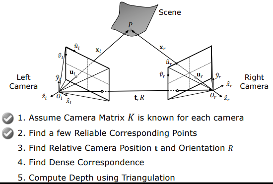
flowchart TD
Step1["1. Obtain Intrinsic Calibration Matrices (K_l, K_r)"] --> Step2["2. Sparse Feature Matching (SIFT/ORB)"]
Step2 --> Step3["3. Estimate Relative Camera Pose (F, E -> R, t)"]
Step3 --> Step4["4. Dense Correspondence Search along Epipolar Lines"]
Step4 --> Step5["5. 3D Depth Computation via Triangulation"]
style Step1 fill:#1a1a2e,stroke:#e94560,color:#fff
style Step2 fill:#16213e,stroke:#4cc9f0,color:#fff
style Step3 fill:#0f3460,stroke:#e94560,color:#fff
style Step4 fill:#1a1a2e,stroke:#4cc9f0,color:#fff
style Step5 fill:#16213e,stroke:#e94560,color:#fff
2.1 Step-by-Step Pipeline Breakdown
- Obtaining Intrinsic Parameters: Intrinsic matrices ($K_l, K_r$) containing focal lengths ($f_x, f_y$) and principal points ($o_x, o_y$) are assumed to be known or extracted from image headers: $$K = \begin{bmatrix} f_x & 0 & o_x \\ 0 & f_y & o_y \\ 0 & 0 & 1 \end{bmatrix}$$
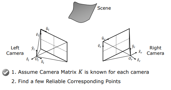
- Sparse Feature Matching: Feature detectors such as SIFT or ORB extract a sparse set of reliable corresponding points $(u_l^{(i)}, v_l^{(i)}) \leftrightarrow (u_r^{(i)}, v_r^{(i)})$ across both images.
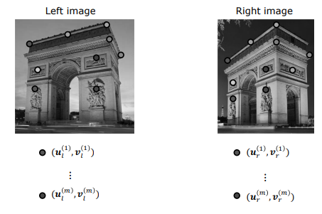
- Relative Pose Estimation: Using the sparse matches, the Fundamental Matrix ($F$) or Essential Matrix ($E$) is computed. Matrix decomposition yields relative rotation ($R$) and translation ($\mathbf{t}$), calibrating the stereo pair ex post facto.
- Dense Correspondence: Epipolar geometry reduces the 2D correspondence search space to 1D epipolar lines. Every pixel in the left image is matched to a corresponding pixel along its epipolar line in the right image.
- 3D Reconstruction via Triangulation: Matched pixel pairs are intersected (triangulated) in 3D space to generate a dense 3D point cloud or depth map.
3. Epipolar Geometry
Epipolar Geometry describes the intrinsic geometric projective relationships between two cameras viewing the same 3D scene point.
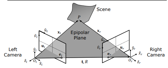
3.1 Geometric Definitions
- Optical Centers ($O_l, O_r$): The pinhole projection centers of the left and right cameras.
- Baseline: The 3D line segment connecting optical centers $O_l$ and $O_r$.
- Epipoles ($e_l, e_r$): The projection of one camera’s optical center onto the image plane of the other camera (where the baseline intersects the image planes).
- Epipolar Plane: The 3D plane formed by a scene point $P$ and the two optical centers ($O_l, O_r$).
- Epipolar Lines: The lines formed by the intersection of the epipolar plane with the left and right image planes. Any pixel $\mathbf{u}_l$ in the left image must have its corresponding match $\mathbf{u}_r$ lie on the corresponding epipolar line in the right image.
Key Insight: The epipolar constraint reduces the 2D correspondence search problem to a 1D line search, reducing computational complexity from $O(W \times H)$ to $O(W)$ while dramatically eliminating false matches.
3.2 Essential Matrix ($E$)
Introduced by H.C. Longuet-Higgins in 1981, the Essential Matrix encapsulates the rigid body transformations between two calibrated views. Let $\mathbf{X}_l$ be the 3D coordinates of point $P$ in the left camera frame, and $\mathbf{X}_r$ in the right camera frame:
$$\mathbf{X}_l = R \mathbf{X}_r + \mathbf{t}$$
The normal vector ($\mathbf{n}$) to the epipolar plane is constructed via the cross product of translation vector $\mathbf{t}$ and position vector $\mathbf{X}_l$:
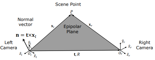
$$\mathbf{n} = \mathbf{t} \times \mathbf{X}_l$$
Because $\mathbf{X}_l$ lies on the epipolar plane, it is orthogonal to the plane normal $\mathbf{n}$, giving the coplanarity constraint:
$$\mathbf{X}_l \cdot (\mathbf{t} \times \mathbf{X}_l) = 0$$
Expressing the vector cross product as matrix multiplication using skew-symmetric matrix $T_\times$:
$$T_\times = \begin{bmatrix} 0 & -t_z & t_y \\ t_z & 0 & -t_x \\ -t_y & t_x & 0 \end{bmatrix}$$
This yields $(\mathbf{X}l - \mathbf{t})^T T\times \mathbf{X}_l = 0 \implies \mathbf{X}r^T R^T T\times \mathbf{X}_l = 0$. Transposing and grouping rotation/translation defines the Essential Matrix ($E$):
$$E = T_\times R$$
$$\mathbf{X}_l^T E \mathbf{X}_r = 0$$
$E$ is a $3 \times 3$ rank-2 matrix with 5 degrees of freedom (3 for rotation, 2 for translation orientation up to scale).
3.3 Fundamental Matrix ($F$)
Developed by Olivier Faugeras and Quang-Tuan Luong in 1992, the Fundamental Matrix generalizes the essential matrix to uncalibrated pixel coordinates.
Because 3D points ($\mathbf{X}_l, \mathbf{X}_r$) are unobservable directly, the essential constraint is converted into 2D pixel coordinates using camera intrinsics ($\mathbf{u}_l = K_l \mathbf{X}_l \implies \mathbf{X}_l = K_l^{-1} \mathbf{u}_l$ and $\mathbf{u}_r = K_r \mathbf{X}_r \implies \mathbf{X}_r = K_r^{-1} \mathbf{u}_r$):
$$(K_l^{-1} \mathbf{u}_l)^T E (K_r^{-1} \mathbf{u}_r) = 0 \implies \mathbf{u}_l^T (K_l^{-T} E K_r^{-1}) \mathbf{u}_r = 0$$
Defining the Fundamental Matrix ($F$):
$$F = K_l^{-T} E K_r^{-1}$$
$$\mathbf{u}_l^T F \mathbf{u}_r = 0$$
The Fundamental Matrix $F$ maps pixel coordinates directly between uncalibrated image pairs without requiring explicit 3D geometry beforehand.
4. Estimating Fundamental Matrix
The standard algorithm for estimating $F$ from point correspondences is the 8-Point Algorithm.
4.1 8-Point Algorithm Formulation
Given point pairs in homogeneous pixel coordinates $\mathbf{u}{li} = [u{li}, v_{li}, 1]^T$ and $\mathbf{u}{ri} = [u{ri}, v_{ri}, 1]^T$, expanding $\mathbf{u}{li}^T F \mathbf{u}{ri} = 0$ yields a linear equation per point pair:
$$u_{li} u_{ri} f_{11} + v_{li} u_{ri} f_{12} + u_{ri} f_{13} + u_{li} v_{ri} f_{21} + v_{li} v_{ri} f_{22} + v_{ri} f_{23} + u_{li} f_{31} + v_{li} f_{32} + f_{33} = 0$$
Stacking equations for $N \ge 8$ point pairs produces the linear system:
$$A \mathbf{f} = \mathbf{0}$$
where $A$ is an $N \times 9$ measurement matrix and $\mathbf{f}$ is the flattened 9-vector of matrix $F$.
4.2 Scale Ambiguity and Constrained Least Squares Solution
Because $F$ operates on homogeneous coordinates, multiplying $F$ by any non-zero scalar $k$ preserves the epipolar constraint ($F \equiv k F$). To fix this scale ambiguity and prevent the trivial solution $\mathbf{f} = \mathbf{0}$, the norm constraint $|\mathbf{f}|^2 = 1$ is imposed:
$$\min_{\mathbf{f}} |A \mathbf{f}|^2 \quad \text{subject to} \quad |\mathbf{f}|^2 = 1$$
The solution vector $\mathbf{f}$ is the eigenvector corresponding to the smallest eigenvalue of $A^T A$, obtained via SVD of $A = U D V^T$ (the last column of $V$).
4.3 Rank-2 Constraint Enforcement and Pose Decomposition
A valid fundamental matrix must satisfy $\det(F) = 0$ (rank 2). To enforce rank 2 on noisy estimates, SVD is applied: $F = U \text{diag}(\sigma_1, \sigma_2, \sigma_3) V^T$. Setting $\sigma_3 = 0$ reconstructs the optimal rank-2 fundamental matrix $F’$.
The Essential Matrix is then recovered via $E = K_l^T F’ K_r$. Decomposing $E$ via SVD yields 4 possible geometric solutions for $(R, \mathbf{t})$. Enforcing the cheirality constraint (requiring reconstructed 3D points to lie in front of both cameras, $z > 0$) uniquely selects the valid physical camera pose.
5. Finding Correspondences
Once $F$ is estimated, dense correspondences across the entire image pair are established.
5.1 Computing Epipolar Lines
For any pixel $\mathbf{u}_l = [u_l, v_l, 1]^T$ in the left image, the corresponding epipolar line coefficients $\mathbf{l}_r = [a, b, c]^T$ in the right image are computed directly via matrix-vector multiplication:
$$\mathbf{l}r = F^T \mathbf{u}l = \begin{bmatrix} f{11} & f{21} & f_{31} \\ f_{12} & f_{22} & f_{32} \\ f_{13} & f_{23} & f_{33} \end{bmatrix} \begin{bmatrix} u_l \\ v_l \\ 1 \end{bmatrix}$$
The matching pixel $(u_r, v_r)$ must lie on the line $a u_r + b v_r + c = 0$.
Numerical Example (from CAVE Monograph)
Consider the numerical example from Columbia CAVE lecture notes:
$$F = \begin{bmatrix} -0.003 & -0.028 & 13.19 \\ -0.003 & -0.008 & -29.2 \\ 2.97 & 56.38 & -9999 \end{bmatrix}, \quad \tilde{\mathbf{u}}_l = \begin{bmatrix} 343 \\ 221 \\ 1 \end{bmatrix}$$
Computing the right epipolar line vector for pixel $(343, 221)$:
$$\mathbf{l}_r = F^T \tilde{\mathbf{u}}_l = \begin{bmatrix} -0.003 & -0.003 & 2.97 \\ -0.028 & -0.008 & 56.38 \\ 13.19 & -29.2 & -9999 \end{bmatrix} \begin{bmatrix} 343 \\ 221 \\ 1 \end{bmatrix} \approx \begin{bmatrix} 0.03 \\ 0.99 \\ -265 \end{bmatrix}$$
This yields the explicit line equation:
$$0.03 u_r + 0.99 v_r - 265 = 0$$
Searching for the match of $(343, 221)$ is thus restricted to this single 1D line in the right image.
5.2 1D Line Search and Template Matching
A local patch centered at $\mathbf{u}_l$ is slid along the 1D epipolar line in the right image. Similarity criteria such as SAD (Sum of Absolute Differences) or NCC (Normalized Cross-Correlation) identify the peak match location.
6. Computing Depth
Having computed dense correspondences, 3D point positions are reconstructed via Triangulation.
6.1 Triangulation via Projection Matrices
Let the projection equations for the left and right cameras be expressed as:
$$\tilde{\mathbf{u}}_l \equiv P_l \tilde{\mathbf{X}}_r, \quad \tilde{\mathbf{u}}r \equiv M{int_r} \tilde{\mathbf{X}}_r$$
where $M_{int_r} = K_r [I \mid \mathbf{0}]$ is the $3 \times 4$ intrinsic projection matrix of the right camera frame, and $P_l = K_l [R \mid \mathbf{t}]$ is the $3 \times 4$ projection matrix of the left camera frame. Expanding the cross-product constraints ($\mathbf{u} \times P \tilde{\mathbf{X}} = \mathbf{0}$) constructs a linear system of 4 equations in 3 unknowns ($x_r, y_r, z_r$):
$$\begin{bmatrix} u_r m_{31} - m_{11} & u_r m_{32} - m_{12} & u_r m_{33} - m_{13} \\ v_r m_{31} - m_{21} & v_r m_{32} - m_{22} & v_r m_{33} - m_{23} \\ u_l p_{31} - p_{11} & u_l p_{32} - p_{12} & u_l p_{33} - p_{13} \\ v_l p_{31} - p_{21} & v_l p_{32} - p_{22} & v_l p_{33} - p_{23} \end{bmatrix} \begin{bmatrix} x_r \\ y_r \\ z_r \end{bmatrix} = \begin{bmatrix} m_{14} - u_r m_{34} \\ m_{24} - v_r m_{34} \\ p_{14} - u_l p_{34} \\ p_{24} - v_l p_{34} \end{bmatrix}$$
$$A_{4 \times 3} \mathbf{x}r = \mathbf{b}{4 \times 1}$$
Solving via pseudo-inverse minimizes squared error:
$$\mathbf{x}_r = (A^T A)^{-1} A^T \mathbf{b}$$
This technique underpins internet-scale Photo Tourism and Structure-from-Motion (SfM) systems.
6.2 Active Illumination for Textureless Surfaces
For textureless or uniform surfaces (e.g., human faces or blank walls), template matching fails due to lack of local contrast. Active Illumination (Zhang et al., 2003) projects artificial spatio-temporally varying stripe or dot patterns onto the scene to enable dense stereo matching.
7. Stereo Vision in Nature (Stereopsis)
Biological vision systems utilize Stereopsis (Greek stereo: solid/3D, opsis: appearance) for natural binocular depth perception.
7.1 Predators vs. Prey
Evolutionary adaptations have placed eyes according to survival requirements:
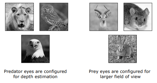
- Predators (Lion, Owl, Eagle): Forward-facing eyes with high binocular overlap. This maximises stereopsis for accurate distance estimation to prey.
- Prey (Gazelle, Mouse, Rabbit): Side-facing eyes with minimal overlap, maximizing total field of view (~360 degrees) for threat detection.
7.2 Human Visual System and Optics
The human interocular distance averages 64 mm. When converging on an object, 6 extraocular muscles rotate the eyes inward (Vergence) to intersect optical axes on the target.
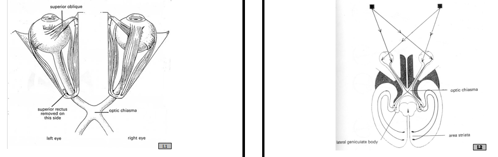
Optic signals cross at the Optic Chiasma and pass through the Lateral Geniculate Nucleus (LGN) to the primary visual cortex (area striata) for binocular depth fusion.
7.3 Psychophysical Experiments and Illusions
Classic experiments demonstrate the mechanisms of visual stereopsis:
Pseudoscope and Telestereoscope
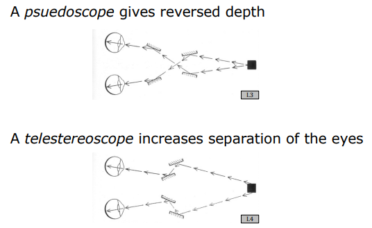
- Pseudoscope: Uses mirrors to swap light paths entering left and right eyes, causing complete depth reversal (convex surfaces appear concave).
- Telestereoscope: Uses periscopic mirrors to artificially widen the effective interocular baseline, dramatically enhancing depth relief of distant objects.
Pulfrich Pendulum Effect (Arden & Weale, 1954)
Placing a dark filter over one eye causes a temporal latency in retinal transmission due to lower photon intensity.
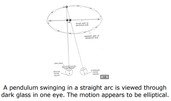
A pendulum swinging in a flat 2D plane appears to travel in a 3D elliptical orbit due to the artificial temporal latency.
Stratton’s Inverted Vision Experiment (1896)
George Stratton wore optical harnesses that inverted his visual field for consecutive days.
Through neural plasticity, his brain adapted to perceive the world upright again within days.
Held & Hein Kitten Experiment (1963) & Pfister’s Chicken Experiment
- Held & Hein (1963): Kittens raised in darkness were placed in a carousel: one walked actively while the other was carried passively. Only the active kitten developed normal depth perception, proving active sensorimotor interaction is mandatory for stereopsis development.
- Pfister’s Chicken (Hess, 1953): Chickens fitted with optical prisms failed to adapt, repeatedly missing food, showing that complex stereo adaptation is restricted to higher evolutionary organisms.
8. Summary Technical Comparison Matrix
| Topic | Primary Mathematical / Physical Logic | Recovered Information | Fundamental Limit / Constraint |
|---|---|---|---|
| Epipolar Geometry | $\mathbf{u}_l^T F \mathbf{u}_r = 0$ | Projective relationship between left & right views. | Failure on smooth, textureless surfaces. |
| Fundamental Matrix Estimation | $A \mathbf{f} = \mathbf{0}, |\mathbf{f}|^2=1$ (SVD / Eigenvector) | Decomposes $F \to E \to R, \mathbf{t}$ under known intrinsics. | Requires at least 8 independent non-coplanar point pairs. |
| Finding Correspondences | $\mathbf{l}_r = F^T \mathbf{u}_l$, 1D Search ($a u_r + b v_r + c = 0$) | Equation of epipolar line corresponding to left pixel. | Geometric distortion (foreshortening) from camera angle differences. |
| Computing Depth | $A_{4 \times 3} \mathbf{x}r = \mathbf{b}{4 \times 1} \implies \mathbf{x}_r = (A^T A)^{-1} A^T \mathbf{b}$ | Precise 3D scene coordinates via least squares triangulation. | Measurement pixel noise creates surface ripples in depth maps. |
| Stereo Vision in Nature | Vergence, LGN routing, Active interaction | Biological depth perception limits and neural adaptation. | Lower organisms cannot adapt to optical distortions. |
Optical Flow and Motion Analysis
- 1. Overview and Historical Foundations
- 2. Motion Field & Optical Flow
- 3. Optical Flow Constraint Equation
- 4. Lucas-Kanade Method
- 5. Coarse-to-Fine Flow Estimation
- 6. Alternative Approach: Template Matching
- 7. Applications of Optical Flow
- 8. Summary & Technical Comparison Matrix
In previous discussions on camera calibration, stereo vision, and shape from shading, scenes or camera systems were predominantly assumed to be stationary. However, the physical world is inherently dynamic: objects move in 3D space, cameras undergo egomotion, and visual motion constitutes one of the most critical sources of information for both biological and artificial perception systems.
This note provides a comprehensive, mathematically rigorous treatment of Optical Flow and Motion Analysis. We cover the physical distinctions between the Motion Field and Optical Flow, the derivation of the Optical Flow Constraint Equation (OFCE), the Aperture Problem, the Lucas-Kanade Least Squares Formulation, condition number analysis via Eigenvalues, multi-scale Coarse-to-Fine Warping Pyramids, Template Matching trade-offs, and key real-world industrial applications.
1. Overview and Historical Foundations
When analyzing dynamic scenes captured across consecutive video frames ($t$ and $t + \delta t$), we seek to measure the visual displacement of pixels over time. In computer vision literature, this problem is framed through two distinct concepts:
- Motion Field ($\mathbf{v}_i$): The 2D velocity vector field in the image plane formed by the geometric perspective projection of the true 3D physical velocities ($\mathbf{v}_0$) of points in the scene.
- Optical Flow ($\mathbf{u}$): The perceived 2D velocity vector field $(u, v)$ of brightness patterns moving across the image sensor array over time.
Our ultimate goal is often to recover the true physical motion field ($\mathbf{v}_i$) from the observable image brightness changes. However, because cameras record only quantized irradiance values (intensities and colors), we can only compute the motion of brightness patterns (optical flow).
flowchart LR
subgraph PhysicalSpace["Physical 3D Space"]
P["3D Scene Point P0(x,y,z)"] -->|Physical Velocity v0| MF["Motion Field (vi)"]
end
subgraph SensorArray["2D Image Plane"]
I["Pixel Intensities I(x,y,t)"] -->|Brightness Displacements| OF["Optical Flow (u,v)"]
end
MF -.->|Identical Under Ideal Conditions| OF
style PhysicalSpace fill:#1a1a2e,stroke:#e94560,color:#fff
style SensorArray fill:#16213e,stroke:#4cc9f0,color:#fff
Key Insight: Under uniform diffuse lighting and richly textured surfaces, optical flow and the motion field coincide. However, specular highlights, moving light sources, and textureless surfaces create fundamental discrepancies where optical flow departs drastically from the true physical motion field.
2. Motion Field & Optical Flow
2.1 Mathematical Derivation of the Motion Field ($\mathbf{v}_i$)
Consider a standard pinhole camera coordinate frame centered at the optical center (Horn, 1981).
Let a 3D scene point $P_0$ have position vector $\mathbf{r}_0 = [x_w, y_w, z_w]^T$. Its perspective projection on the image plane is point $p_i$ with position vector $\mathbf{r}_i = [x_i, y_i, f]^T$.
Given the camera focal length $f$ and optical axis unit vector $\mathbf{z}$, perspective projection yields:
$$\mathbf{r}_i = f \frac{\mathbf{r}_0}{\mathbf{r}_0 \cdot \mathbf{z}}$$
where $\mathbf{r}_0 \cdot \mathbf{z} = z_w$ is the 3D depth of the point along the optical axis.
If the 3D point moves with instantaneous physical velocity $\mathbf{v}_0 = \frac{d\mathbf{r}_0}{dt}$, the resulting image velocity—the Motion Field $\mathbf{v}_i$—is obtained by taking the time derivative:
$$\mathbf{v}_i = \frac{d\mathbf{r}_i}{dt}$$
Applying the quotient rule of differential calculus:
$$\mathbf{v}_i = \frac{d}{dt} \left( f \frac{\mathbf{r}_0}{\mathbf{r}_0 \cdot \mathbf{z}} \right) = f \frac{(\mathbf{r}_0 \cdot \mathbf{z})\mathbf{v}_0 - \mathbf{r}_0 (\mathbf{v}_0 \cdot \mathbf{z})}{(\mathbf{r}_0 \cdot \mathbf{z})^2}$$
Using the vector triple product identity $\mathbf{a} \times (\mathbf{b} \times \mathbf{c}) = (\mathbf{a} \cdot \mathbf{c})\mathbf{b} - (\mathbf{a} \cdot \mathbf{b})\mathbf{c}$, we can write the motion field equation in compact vector form:
$$\mathbf{v}_i = f \frac{(\mathbf{r}_0 \times \mathbf{v}_0) \times \mathbf{z}}{(\mathbf{r}_0 \cdot \mathbf{z})^2} = \frac{f \cdot (\mathbf{z} \times (\mathbf{r}_0 \times \mathbf{v}_0))}{(\mathbf{r}_0 \cdot \mathbf{z})^2}$$
This formula analytically maps a known 3D point position ($\mathbf{r}_0$), depth ($z_w$), and 3D velocity ($\mathbf{v}_0$) to the exact geometric velocity vector ($\mathbf{v}_i$) in the image plane.
2.2 Boundary Scenarios Where Optical Flow $\neq$ Motion Field
While we want optical flow to equal the true motion field, optical reflection laws and lighting dynamics lead to three classic failure modes:
1. Motion Field Exists, No Optical Flow (Spinning Sphere)
- Scenario: A perfectly smooth, textureless sphere rotates about its central vertical axis under fixed point lighting.
- Analysis: Because the physical matter is rotating, physical points possess velocity ($\mathbf{v}_0 \neq \mathbf{0}$); thus, a non-zero motion field exists. However, because the surface is completely uniform and the light source is stationary, the recorded shading and intensities do not change over time ($\frac{\partial I}{\partial t} = 0$). Consecutive frames are identical. Thus, optical flow is identically zero.
2. No Motion Field, Optical Flow Exists (Moving Light Source)
- Scenario: A smooth sphere is held completely stationary ($\mathbf{v}_0 = \mathbf{0}$), but the light source illuminating it orbits around the sphere.
- Analysis: Because the sphere is static, the motion field is zero. However, the moving light shifts the specular highlight, terminator boundary, and shading gradients across the sensor. The camera detects moving brightness patterns; thus, optical flow is non-zero.
3. Orthogonal Directions (Barber Pole Illusion)
- Scenario: A classic barber shop pole (cylinder) painted with diagonal helical stripes rotates about its vertical axis.
- Analysis: Every physical point on the cylinder rotates horizontally (horizontal motion field). However, human perception and differential cameras track the continuous diagonal stripes translating purely vertically (vertical optical flow). The motion field and optical flow vectors are mutually perpendicular (orthogonal, $90^\circ$ mismatch).
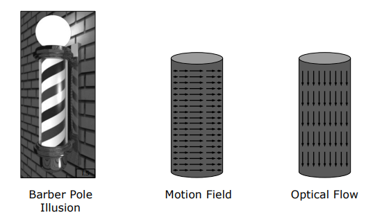
2.3 Optical Flow Illusions in Human Psychophysics
The human visual cortex (particularly area MT / V5) interprets temporal brightness gradients as physical motion, giving rise to fascinating psychophysical motion illusions:
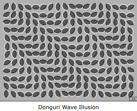
- Donguri Wave Illusion: A static 2D arrangement of acorn/leaf patterns with asymmetric luminance transitions. Micro-saccadic eye movements trigger differential temporal filters, inducing the sensation of moving waves across a static page.
- Ouchi Pattern: A circular grating surrounded by an orthogonal grating; eye drift creates an apparent relative sliding motion between the central disk and the background.
3. Optical Flow Constraint Equation
Given two consecutive video frames ($t$ and $t + \delta t$), we seek to compute the local displacement $(u, v)$ for every pixel.
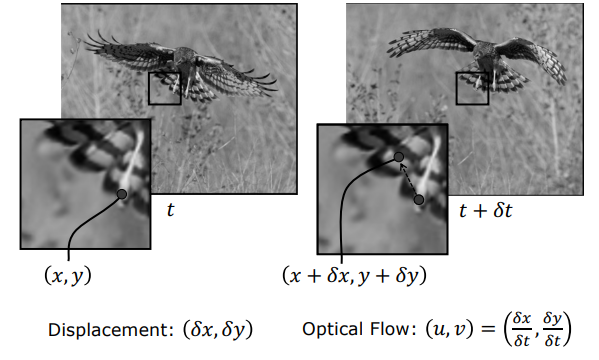
3.1 Fundamental Assumptions
The mathematical formulation rests on two core assumptions:
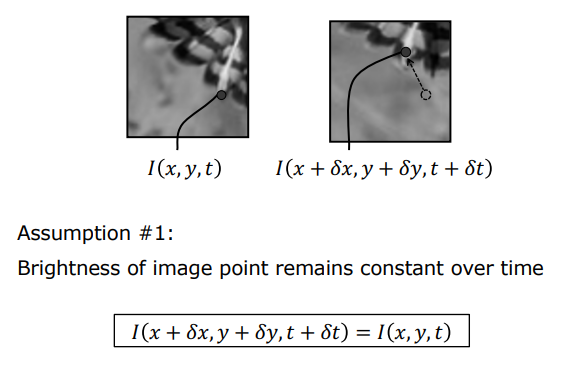
- Brightness Constancy Assumption: The irradiance of a scene point projected onto the sensor remains constant over small time intervals: $$I(x, y, t) = I(x + \delta x, y + \delta y, t + \delta t)$$
- Small Motion / Displacement Assumption: The temporal step $\delta t$ is small enough that spatial displacements $\delta x, \delta y$ are infinitesimal ($\delta x, \delta y \ll 1$ pixel), enabling first-order Taylor series approximation.
3.2 Taylor Series Expansion and Differential Derivation
Expanding $I(x + \delta x, y + \delta y, t + \delta t)$ via multi-variable Taylor series around $(x, y, t)$:
$$I(x + \delta x, y + \delta y, t + \delta t) \approx I(x, y, t) + \frac{\partial I}{\partial x}\delta x + \frac{\partial I}{\partial y}\delta y + \frac{\partial I}{\partial t}\delta t + \mathcal{O}(\delta^2)$$
Neglecting higher-order terms $\mathcal{O}(\delta^2)$ and substituting the Brightness Constancy condition:
$$I_x \delta x + I_y \delta y + I_t \delta t = 0$$
where $I_x = \frac{\partial I}{\partial x}$, $I_y = \frac{\partial I}{\partial y}$, and $I_t = \frac{\partial I}{\partial t}$.
Dividing both sides by $\delta t$ and taking the limit $\delta t \to 0$:
$$I_x \frac{dx}{dt} + I_y \frac{dy}{dt} + I_t = 0$$
Defining horizontal velocity $u = \frac{dx}{dt}$ and vertical velocity $v = \frac{dy}{dt}$, we obtain the celebrated Optical Flow Constraint Equation (OFCE):
$$I_x u + I_y v + I_t = 0 \quad \iff \quad \nabla I \cdot \mathbf{u} + I_t = 0$$
where $\nabla I = [I_x, I_y]^T$ is the spatial image gradient and $\mathbf{u} = [u, v]^T$ is the optical flow velocity vector.
3.3 Spatio-Temporal Finite Differences
The gradients $I_x, I_y, I_t$ are evaluated numerically from consecutive image frames using a $2 \times 2 \times 2$ spatio-temporal pixel cube (Horn & Schunck, 1981):
$$I_x(k, l, t) \approx \frac{1}{4} \Big[ I(k+1, l, t) + I(k+1, l, t+1) + I(k+1, l+1, t) + I(k+1, l+1, t+1) \Big] - \frac{1}{4} \Big[ I(k, l, t) + I(k, l, t+1) + I(k, l+1, t) + I(k, l+1, t+1) \Big]$$
Corresponding symmetric averages compute $I_y(k, l, t)$ and $I_t(k, l, t)$.
3.4 Geometric Interpretation and the Aperture Problem
The constraint $I_x u + I_y v + I_t = 0$ defines a straight constraint line in the $u-v$ velocity space.
One Equation, Two Unknowns
For each pixel, we have 1 scalar equation with 2 unknowns ($u$ and $v$). The system is inherently under-constrained, and any point along the constraint line satisfies the equation.
The velocity vector can be resolved into two orthogonal components:
$$\mathbf{u} = \mathbf{u}_n + \mathbf{u}_p$$
- Normal Flow ($\mathbf{u}_n$): Perpendicular to the constraint line (parallel to spatial gradient $\nabla I$). Its magnitude and direction are uniquely determined: $$\hat{\mathbf{u}}_n = \frac{[I_x, I_y]^T}{\sqrt{I_x^2 + I_y^2}}, \quad |\mathbf{u}_n| = \frac{-I_t}{\sqrt{I_x^2 + I_y^2}} \implies \mathbf{u}_n = -\frac{I_t}{I_x^2 + I_y^2} \begin{bmatrix} I_x \ I_y \end{bmatrix}$$
- Parallel Flow ($\mathbf{u}_p$): Tangent to the constraint line (along the edge contour). It cannot be determined from a single pixel observation.
The Aperture Problem: When viewing a moving 1D edge through a local circular aperture, motion parallel to the edge generates no intensity change. Only motion perpendicular to the edge (normal flow) is observable. Resolving the true 2D velocity requires 2D features (corners, textured patches) or spatial neighborhood constraints.
4. Lucas-Kanade Method
Bruce Lucas and Takeo Kanade (1981) introduced a landmark solution by imposing a local spatial consistency constraint.
4.1 Spatial Coherence Assumption
The Lucas-Kanade method assumes that all pixels within a small spatial window $W$ ($n \times n$, typically $3 \times 3$ or $5 \times 5$) around the target pixel move with the same identical velocity:
$$\mathbf{u}(x, y) = [u, v]^T = \text{const} \quad \forall (x,y) \in W$$
For an $n \times n$ window containing $n^2$ pixels, evaluating the OFCE at each pixel yields an overdetermined system of $n^2$ equations in 2 unknowns:
$$\begin{aligned} I_{x1} u + I_{y1} v &= -I_{t1} \ I_{x2} u + I_{y2} v &= -I_{t2} \ &;;\vdots \ I_{xn^2} u + I_{yn^2} v &= -I_{tn^2} \end{aligned}$$
4.2 Matrix Formulation and Least Squares Solution
Expressing this linear system in matrix form:
$$A \mathbf{u} = \mathbf{b}$$
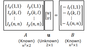
where:
- $A = \begin{bmatrix} I_{x1} & I_{y1} \ I_{x2} & I_{y2} \ \vdots & \vdots \ I_{xn^2} & I_{yn^2} \end{bmatrix}$ is the $n^2 \times 2$ spatial gradient matrix.
- $\mathbf{u} = \begin{bmatrix} u \ v \end{bmatrix}$ is the $2 \times 1$ unknown velocity vector.
- $\mathbf{b} = \begin{bmatrix} -I_{t1} \ -I_{t2} \ \vdots \ -I_{tn^2} \end{bmatrix}$ is the $n^2 \times 1$ temporal derivative vector.
Solving via the pseudo-inverse / Least Squares:
$$A^T A \mathbf{u} = A^T \mathbf{b} \implies \mathbf{u} = (A^T A)^{-1} A^T \mathbf{b}$$
Expanding the matrix components into a compact $2 \times 2$ system:
$$\begin{bmatrix} \sum I_x^2 & \sum I_x I_y \ \sum I_x I_y & \sum I_y^2 \end{bmatrix} \begin{bmatrix} u \ v \end{bmatrix} = \begin{bmatrix} -\sum I_x I_t \ -\sum I_y I_t \end{bmatrix}$$
where all summations $\sum$ run over all pixels in window $W$. Note that $M = A^T A$ is identical in form to the Harris corner structure tensor.
4.3 Well-Conditioning Analysis via Eigenvalues
For $(A^T A)^{-1}$ to exist stably without numerical noise amplification, $M = A^T A$ must be well-conditioned. This is governed by its eigenvalues $\lambda_1, \lambda_2$:
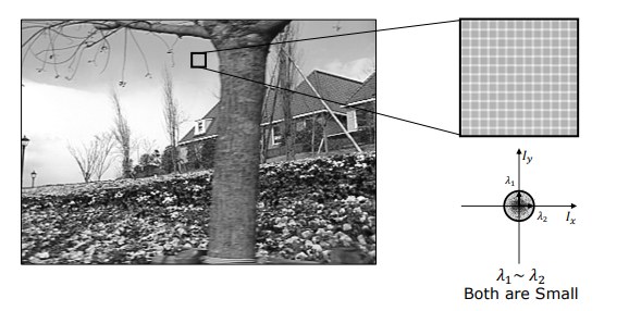
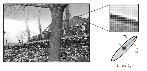
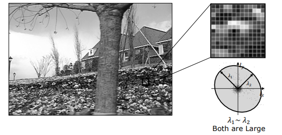
| Region Characteristics | Gradient Distribution (Ellipse) | Eigenvalue Status ($\lambda_1, \lambda_2$) | Matrix Conditioning | Flow Estimation Quality |
|---|---|---|---|---|
| Textureless Area (e.g., Sky) | Small cluster concentrated at origin | $\lambda_1 \approx 0, ; \lambda_2 \approx 0$ | Badly Conditioned: Singular, non-invertible matrix. | Unsolvable: Division by zero or massive noise amplification. |
| Straight Edge (e.g., Roofline) | Thin, elongated ellipse along edge normal | $\lambda_1 \gg \lambda_2$ ($\lambda_2 \approx 0$) | Badly Conditioned: Gradient in one direction only (Aperture Problem). | Partial: Only normal flow is recoverable; parallel component is ambiguous. |
| Textured / Corner Area (e.g., Flowers) | Broad circular/oval spread across both axes | $\lambda_1, \lambda_2 \gg 0$ ($\lambda_1 \sim \lambda_2$) | Well-Conditioned: Invertible with high numerical stability. | Excellent: 2D optical flow $(u, v)$ uniquely and accurately solved. |
5. Coarse-to-Fine Flow Estimation
Because the Lucas-Kanade derivation relies on first-order Taylor expansion, it strictly requires sub-pixel or near-pixel displacements ($\delta x, \delta y \ll 1$). In real videos, fast-moving objects or camera motion can cause displacements of 20 to 50 pixels per frame, violating linearity and breaking the OFCE ($I_x u + I_y v + I_t \neq 0$).
To overcome this limitation, a multi-scale Gaussian Resolution Pyramid and Warping framework is employed (Bouguet, 2000).
5.1 Resolution Pyramid Concept
- A hierarchy of downsampled images is built by successive $2 \times 2$ spatial averaging: $N \times N$, $N/2 \times N/2$, $N/4 \times N/4$, $N/8 \times N/8$.
- Key Mathematical Invariance: A large displacement of 16 pixels at full resolution becomes exactly 1 pixel at the $N/16 \times N/16$ level!
- At the coarsest level, motion falls within the linear Taylor regime, allowing standard Lucas-Kanade to function reliably.
5.2 Step-by-Step Algorithm (Bouguet 2000)
flowchart TD
A["Level L (Coarsest Pyramid Level)"] -->|Standard LK| B["Compute Initial Coarse Flow (u0, v0)"]
B --> C["Upscale & Multiply Flow by 2 (Level L-1)"]
C --> D["Warp Frame t towards Frame t+dt using Upscaled Flow"]
D -->|Residual Displacement < 1 px| E["Solve Residual Flow (du, dv) via LK on Warped Image"]
E --> F["Accumulate Flow: u = 2*u_prev + du"]
F --> G{"Reached Base Resolution (L=0)?"}
G -- No --> C
G -- Yes --> H["Final High-Accuracy Optical Flow Field"]
style A fill:#1a1a2e,stroke:#e94560,color:#fff
style D fill:#16213e,stroke:#4cc9f0,color:#fff
style H fill:#0f3460,stroke:#2ecc71,color:#fff
- Coarse Initialization: At the lowest resolution (pyramid apex), compute initial flow $\mathbf{u}^{(0)}$ using standard Lucas-Kanade.
- Upscaling: Pass the flow field to the next higher-resolution level, scaling velocity coordinates by 2 ($2\mathbf{u}^{(0)}$).
- Backward Image Warping: Warp frame $I(t)$ using the upscaled flow field toward $I(t+\delta t)$, effectively neutralizing the large macroscopic shift.
- Residual Flow Computation: Because warping removes the large motion, the remaining difference between the warped image and $I(t+\delta t)$ is small ($\ll 1$ pixel). Standard Lucas-Kanade solves the residual flow $\Delta \mathbf{u}$.
- Accumulation: Update total flow: $\mathbf{u} = 2\mathbf{u}_{\text{prev}} + \Delta \mathbf{u}$.
- Iterate to Base: Repeat until reaching original image resolution.
6. Alternative Approach: Template Matching
Optical flow can also be approached through direct window-based correlation / template matching rather than differential derivatives:
- Mechanism: A patch $T$ around a pixel in frame $t$ is exhaustively searched across a bounding window $S$ in frame $t+\delta t$, minimizing Sum of Squared Differences ($\min \text{SSD}$) or maximizing Normalized Cross-Correlation ($\max \text{NCC}$).
- Key Drawbacks:
- Prohibitive Computational Cost: Performing 2D exhaustive spatial cross-correlations per pixel is orders of magnitude slower than differential gradient approaches.
- False Matching in Repetitive Textures: Lacking continuous gradient constraints, template matching is prone to latching onto distant, visually similar patterns.
7. Applications of Optical Flow
Optical flow is one of the most widely commercialized algorithms in computer vision, powering critical technologies across industries.
7.1 Optical Mouse
Every standard optical computer mouse houses a high-speed embedded computer vision pipeline:
- An LED/laser illuminates microscopic surface imperfections on the desk.
- A tiny CMOS sensor ($64 \times 64$ pixels) captures images at 1500 to 3000+ FPS.
- An on-board Digital Signal Processor (DSP) executes real-time optical flow / correlation algorithms to compute instantaneous $\Delta x, \Delta y$ velocity vectors, driving the screen cursor.
7.2 Traffic Monitoring & Speed Enforcement
Stationary highway cameras utilize calibrated optical flow for automated velocity measurement:
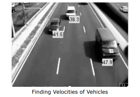
- The camera’s perspective matrix and road plane metric geometry are pre-calibrated.
- Optical flow tracks vehicle bounding patches across frames.
- 2D pixel velocities are directly mapped to physical metric speeds ($\text{km/h}$ or $\text{mph}$).
7.3 Digital Video Stabilization
Smartphones and action cameras apply optical flow to eliminate unwanted handheld camera shake:
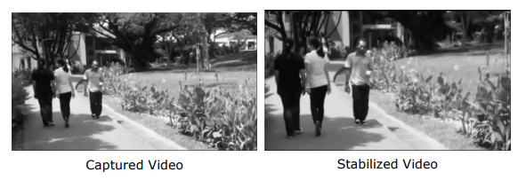
- Hand vibrations induce a coherent global optical flow field across the frame.
- The algorithm isolates the dominant flow field corresponding to the static background.
- Video frames are dynamically warped in the inverse direction of the dominant shake, yielding rock-solid output.
7.4 Other Prominent Industrial Applications
- Video Retiming & Slow-Motion Interpolation: High-precision optical flow interpolates pixel trajectories between adjacent frames ($t$ and $t+1$), synthesizing intermediate sub-frames ($t+0.5$). A standard 30 FPS video can thus be converted to cinematic 240 FPS slow-motion.
- Facial Mesh & Micro-Expression Tracking: Tracking dense 3D mesh vertices across video sequences via optical flow enables millimetric quantification of eye blinks, lip micro-movements, and emotional valence in medical and VFX pipelines.
- Interactive Gaming & Motion Interfaces: Optical flow vector fields extracted from player movements are translated into virtual physical forces (e.g., aerodynamic drag or fluid push on virtual game objects).
8. Summary & Technical Comparison Matrix
| Concept / Technique | Core Mathematical Formulation | Primary Role & Strength | Inherent Limitation / Constraint |
|---|---|---|---|
| Motion Field | $\mathbf{v}_i = \frac{f \cdot (\mathbf{z} \times (\mathbf{r}_0 \times \mathbf{v}_0))}{(\mathbf{r}_0 \cdot \mathbf{z})^2}$ | 2D geometric projection of true 3D physical velocity | Cannot be directly captured by a sensor; requires 3D depth and velocity knowledge. |
| Optical Flow Constraint Equation | $I_x u + I_y v + I_t = 0$ | Relates measurable spatio-temporal image derivatives to velocity $(u, v)$ | Aperture Problem: 1 equation, 2 unknowns; parallel motion component is lost. |
| Lucas-Kanade Least Squares | $\mathbf{u} = (A^T A)^{-1} A^T \mathbf{b}$ | Closed-form local least-squares solution assuming spatial coherence | Fails on textureless regions and straight edges where $A^T A$ is singular / ill-conditioned. |
| Coarse-to-Fine Warping | Pyramids + Warping + $\mathbf{u} = 2\mathbf{u}_{\text{prev}} + \Delta\mathbf{u}$ | Extends differential LK to large displacements by multi-scale downsampling | Prone to interpolation blur and high cumulative computational overhead across layers. |
| Template Matching | $\min \text{SSD}$ or $\max \text{NCC}$ | Window-based correlation without requiring differentiable gradients | Computationally prohibitive for dense fields; vulnerable to false matches in repeating textures. |
Structure from Motion and Tomasi-Kanade Factorization
- 1. Overview and Historical Foundations
- 2. The Structure from Motion Problem (SfM Problem)
- 3. Constructing the Observation Matrix
- 4. Rank of the Observation Matrix
- 5. The Tomasi-Kanade Factorization Algorithm
- 6. Algorithmic Comparison Matrix
- 7. Results, Dense Reconstruction, and Modern SfM Extensions
- 8. Summary of Key Concepts
One of the most elegant, powerful, and mathematically profound achievements in computer vision is the simultaneous recovery of both the 3D geometric structure of a scene and the 3D motion trajectory of the camera from an uncalibrated casual video stream.
This chapter presents a comprehensive, mathematically rigorous treatment of the Structure from Motion (SfM) problem and the seminal Tomasi-Kanade Factorization Algorithm introduced by Carlo Tomasi and Takeo Kanade (1992). We explore the formulation of the Observation Matrix, the algebraic beauty of the Centering Trick, the fundamental Rank Theorem, noise filtering via Singular Value Decomposition (SVD), and the resolution of the affine ambiguity via Orthonormality Constraints to extract the metric transformation matrix $Q$.
1. Overview and Historical Foundations
In classical calibrated stereo and multi-view systems, the geometric relationship between cameras (baseline $b$, rotation matrix $R$, translation vector $\mathbf{t}$) is either calibrated beforehand or determined via pairwise epipolar geometry. However, traditional setups require rigid, pre-calibrated multi-camera rigs or are constrained to two stationary viewpoints.
Structure from Motion (SfM) removes these constraints entirely, solving a far more general and powerful reconstruction problem:
- Casual Video Stream: The input is a single video sequence ($F$ frames) recorded by an uncalibrated, handheld moving camera where camera motion parameters (rotations and translations) are completely unknown a priori.
- Simultaneous Estimation: Without any auxiliary sensors, calibration targets, or depth hardware, the algorithm simultaneously estimates:
- The 3D metric coordinate point cloud of the scene (Scene Structure - $S$),
- The 3D orientation and motion path of the camera across all frames (Camera Motion - $M$).
flowchart TD
subgraph Input["Input (Video Stream)"]
V["Single Handheld Video Sequence (F Frames)"]
end
subgraph Tracking["Feature Tracking"]
F1["Corner / SIFT / Harris Detection"] --> F2["Feature Tracking across Frames (N Points)"]
end
subgraph Factorization["Tomasi-Kanade Factorization"]
W["Observation Matrix (W: 2F x N)"] --> C["Centering Trick (Eliminates Camera Centers)"]
C --> SVD["SVD & Rank-3 Truncation (Eckart-Young)"]
SVD --> Q["Metric Rectification via Orthonormality (Q)"]
end
subgraph Output["Output (3D Reconstruction)"]
M["Camera Motion (M: 2F x 3)"]
S["3D Scene Structure (S: 3 x N)"]
end
Input --> Tracking --> Factorization
Q --> M
Q --> S
style Input fill:#1a1a2e,stroke:#e94560,color:#fff
style Tracking fill:#16213e,stroke:#4cc9f0,color:#fff
style Factorization fill:#0f3460,stroke:#e94560,color:#fff
style Output fill:#1b262c,stroke:#00b4d8,color:#fff
In 1992, Carlo Tomasi and Takeo Kanade introduced a landmark factorization method based on an orthographic camera model. They proved that when centroid-subtracted 2D feature trajectories are stacked into a massive $2F \times N$ Observation Matrix ($W$), the matrix has an algebraic rank of at most 3 (The Rank Theorem).
This rank constraint allows the matrix to be directly decomposed into the product of camera motion and scene structure using Singular Value Decomposition (SVD). Today, this foundational theorem underpins modern visual SLAM (Simultaneous Localization and Mapping), photogrammetry, and internet-scale 3D scene reconstruction algorithms (e.g., COLMAP, Bundler).
Key Insight: Regardless of how many frames are captured ($F \gg 3$) or how many feature points are tracked ($N \gg 3$), the noise-free observation matrix resides in a compact 3-dimensional linear subspace. This low-rank property allows simultaneous global noise suppression and closed-form factorization.
2. The Structure from Motion Problem (SfM Problem)
The input to the orthographic SfM algorithm is an image sequence of a rigid scene captured by a moving camera. The mathematical formulation begins with feature tracking and camera projection modeling.
2.1 Feature Detection and Tracking
To establish correspondences across the entire video sequence:
- Feature Detection: Salient and repeatable interest points (e.g., Harris corners, SIFT keypoints, or Kanade-Lucas-Tomasi / KLT features) are detected in the initial frame.
- Feature Tracking: These points are continuously tracked across all consecutive video frames using template matching, optical flow (Lucas-Kanade), or descriptor matching.
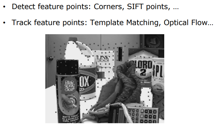
The output of the tracking stage is a set of 2D image coordinates for $N$ scene points observed across $F$ frames:
$$\left\{ (u_{f,p}, v_{f,p}) \right\} \quad \text{where} \quad f \in \{1, \dots, F\} \quad \text{and} \quad p \in \{1, \dots, N\}$$
2.2 Orthographic Camera Assumption
To convert the non-linear perspective projection into a tractable linear formulation, the Tomasi-Kanade algorithm assumes an Orthographic (Parallel Projection) Camera Model.
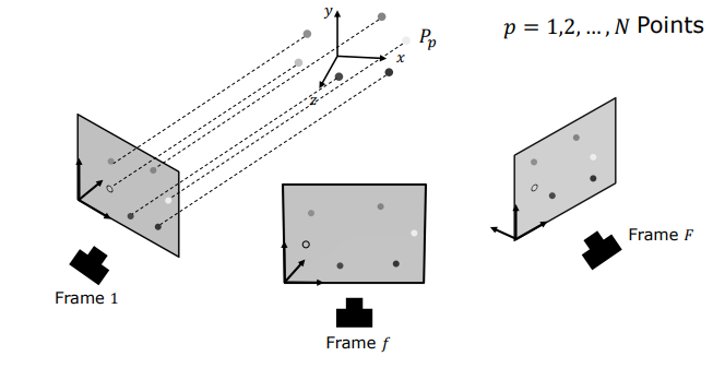
This assumption is physically well-justified under the following conditions:
-
Shallow Depth Variation: When the variation in depth across the object ($\Delta z$) is much smaller than the average distance from the camera to the object ($Z_0$), i.e., $\Delta z \ll Z_0$:
$$\frac{\Delta z}{Z_0} \approx 0 \implies \text{Perspective Scale Factor} \approx \text{Constant}$$
-
Constant Magnification: All points on the object experience approximately identical magnification, making perspective foreshortening negligible.
-
Parallel Projection Rays: Projection rays are parallel lines orthogonal to the image plane rather than converging at a single pinhole focal point.
3. Constructing the Observation Matrix
Let us mathematically analyze how a 3D scene point projects onto the 2D image plane under orthography.
3.1 Orthographic Projection in Camera Coordinates
Let the origin of the camera coordinate frame be located at the camera center $C$. We define two orthonormal unit vectors, $\mathbf{i}$ (horizontal row direction) and $\mathbf{j}$ (vertical column direction), aligned with the sensor coordinate axes.
Let $\mathbf{x}_c$ be the position vector of a 3D scene point $P$ in the camera frame. Under orthographic projection, the pixel coordinates $(u, v)$ on the image plane are given by the dot products of $\mathbf{x}_c$ with the unit directional vectors $\mathbf{i}$ and $\mathbf{j}$:
$$u = \mathbf{i} \cdot \mathbf{x}_c = \mathbf{i}^T \mathbf{x}_c$$
$$v = \mathbf{j} \cdot \mathbf{x}_c = \mathbf{j}^T \mathbf{x}_c$$
3.2 Transition to the World Coordinate Frame
Now consider a fixed world coordinate frame ($\mathcal{W}$) with an arbitrary origin $O$.
- The 3D position of scene point $p$ in world coordinates is $P_p = \mathbf{x}_w$.
- The 3D physical position of the camera center for frame $f$ in world coordinates is $C_f = \mathbf{c}_w$.
By vector subtraction, the camera-relative position vector is:
$$\mathbf{x}_c = \mathbf{x}_w - \mathbf{c}_w = P_p - C_f$$
Substituting this into our projection equations yields the observed 2D coordinates of point $p$ in frame $f$:
$$u_{f,p} = \mathbf{i}_f^T (P_p - C_f) = \mathbf{i}_f^T P_p - \mathbf{i}_f^T C_f$$
$$v_{f,p} = \mathbf{j}_f^T (P_p - C_f) = \mathbf{j}_f^T P_p - \mathbf{j}_f^T C_f$$
Here:
- $P_p \in \mathbb{R}^3$: Unknown 3D coordinates of scene point $p$ ($p = 1, \dots, N$).
- $\mathbf{i}_f, \mathbf{j}_f \in \mathbb{R}^3$: Unknown 3D camera orientation unit vectors for frame $f$ ($f = 1, \dots, F$).
- $C_f \in \mathbb{R}^3$: Unknown 3D camera position for frame $f$ ($f = 1, \dots, F$).
3.3 Multi-Frame Geometry and Unknown Parameters
In this system, we have $2FN$ measured pixel coordinates $(u_{f,p}, v_{f,p})$. However, the camera translations $C_f$ introduce redundant translational parameters coupled with the orientations. To decouple camera translations from rotations and 3D structure, Tomasi and Kanade introduced the Centering Trick.
3.4 The Centering Trick (Eliminating Camera Positions)
Since the world coordinate origin can be placed anywhere without loss of generality, we place the world origin directly at the 3D Centroid ($\bar{P}$) of all $N$ scene points.
Under this choice of origin:
$$\sum_{p=1}^N P_p = \mathbf{0} \iff \frac{1}{N}\sum_{p=1}^N P_p = \mathbf{0}$$
Now, let us compute the 2D image centroid $(\bar{u}_f, \bar{v}_f)$ of all tracked points in frame $f$:
$$\bar{u}_f = \frac{1}{N} \sum_{p=1}^N u_{f,p} = \frac{1}{N} \sum_{p=1}^N \left( \mathbf{i}_f^T P_p - \mathbf{i}_f^T C_f \right)$$
Splitting this summation:
$$\bar{u}_f = \mathbf{i}_f^T \left( \frac{1}{N} \sum_{p=1}^N P_p \right) - \frac{1}{N} \sum_{p=1}^N \left( \mathbf{i}_f^T C_f \right)$$
Because $\sum P_p = \mathbf{0}$, the first term vanishes completely. The second term is independent of $p$, simplifying directly to:
$$\bar{u}_f = -\mathbf{i}_f^T C_f \quad \text{and similarly} \quad \bar{v}_f = -\mathbf{j}_f^T C_f$$
Subtracting these frame centroids from the raw pixel measurements yields the centroid-subtracted coordinates $(\tilde{u}{f,p}, \tilde{v}{f,p})$:
$$\tilde{u}_{f,p} = u_{f,p} - \bar{u}_f = \left( \mathbf{i}_f^T P_p - \mathbf{i}_f^T C_f \right) - \left( -\mathbf{i}_f^T C_f \right) = \mathbf{i}_f^T P_p$$
$$\tilde{v}_{f,p} = v_{f,p} - \bar{v}_f = \left( \mathbf{j}_f^T P_p - \mathbf{j}_f^T C_f \right) - \left( -\mathbf{j}_f^T C_f \right) = \mathbf{j}_f^T P_p$$
Key Theoretical Breakthrough: The centering trick completely eliminates the unknown camera translation vectors $C_f$ from the system! We are left with purely bilinear equations involving only camera orientations ($\mathbf{i}_f, \mathbf{j}_f$) and 3D structure ($P_p$):
$$\tilde{u}_{f,p} = \mathbf{i}_f^T P_p \quad \text{and} \quad \tilde{v}_{f,p} = \mathbf{j}_f^T P_p$$
3.5 Matrix Formulation: $W = M \cdot S$
Collecting all centered coordinates across all $F$ frames and all $N$ points into a single matrix gives the fundamental factorization equation.
For each frame $f$ and point $p$:
$$\begin{bmatrix} \tilde{u}_{f,p} \\ \tilde{v}_{f,p} \end{bmatrix} = \begin{bmatrix} \mathbf{i}_f^T \\ \mathbf{j}_f^T \end{bmatrix} P_p$$
Stacking all entries:
$$\mathbf{W}_{2F \times N} = \mathbf{M}_{2F \times 3} \cdot \mathbf{S}_{3 \times N}$$
1. Observation Matrix ($W$)
The $2F \times N$ matrix of known, centered 2D point tracks:
$$W = \left[ \begin{array}{cccc} \tilde{u}_{1,1} & \tilde{u}_{1,2} & \dots & \tilde{u}_{1,N} \\ \tilde{u}_{2,1} & \tilde{u}_{2,2} & \dots & \tilde{u}_{2,N} \\ \vdots & \vdots & \ddots & \vdots \\ \tilde{u}_{F,1} & \tilde{u}_{F,2} & \dots & \tilde{u}_{F,N} \\ \hline \tilde{v}_{1,1} & \tilde{v}_{1,2} & \dots & \tilde{v}_{1,N} \\ \tilde{v}_{2,1} & \tilde{v}_{2,2} & \dots & \tilde{v}_{2,N} \\ \vdots & \vdots & \ddots & \vdots \\ \tilde{v}_{F,1} & \tilde{v}_{F,2} & \dots & \tilde{v}_{F,N} \end{array} \right]_{2F \times N}$$
2. Camera Motion Matrix ($M$)
The $2F \times 3$ matrix of unknown camera orientation vectors:
$$M = \left[ \begin{array}{c} \mathbf{i}_1^T \\ \mathbf{i}_2^T \\ \vdots \\ \mathbf{i}_F^T \\ \hline \mathbf{j}_1^T \\ \mathbf{j}_2^T \\ \vdots \\ \mathbf{j}_F^T \end{array} \right]_{2F \times 3}$$
3. Scene Structure Matrix ($S$)
The $3 \times N$ matrix of unknown 3D scene point coordinates:
$$S = \begin{bmatrix} P_1 & P_2 & \dots & P_N \end{bmatrix}_{3 \times N}$$
4. Rank of the Observation Matrix
The core discovery that enables Tomasi-Kanade factorization is the algebraic rank property of $W$.
4.1 Linear Independence and Vector Spaces (Math Primer)
A set of vectors is linearly independent if no vector in the set can be written as a linear combination of the others.
- In a 2D plane, at most 2 linearly independent vectors can exist. Any third vector is necessarily linearly dependent.
- In 3D space, at most 3 linearly independent vectors can exist.
4.2 Matrix Rank and Dimensional Bounds
For an $m \times n$ matrix $A$:
- Column Rank: Maximum number of linearly independent columns.
- Row Rank: Maximum number of linearly independent rows.
Fundamental linear algebra establishes that column rank equals row rank:
$$\text{ColumnRank}(A) = \text{RowRank}(A) = \text{Rank}(A) \leq \min(m, n)$$
Furthermore, the rank of a matrix product is bounded by the individual ranks:
$$\text{Rank}(A \cdot B) \leq \min(\text{Rank}(A), \text{Rank}(B))$$
4.3 Rank Geometry in 3D Space
Let us visualize the geometric meaning of rank for a $3 \times 3$ matrix $A = [\mathbf{a} \ \mathbf{b} \ \mathbf{c}]$:
Rank 1 (1D Line)
All column vectors are collinear (scalar multiples of one another), spanning only a 1D line:
Rank 2 (2D Plane)
Column vectors are coplanar, spanning a 2D plane:
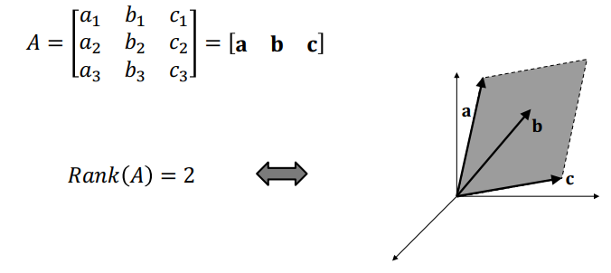
Rank 3 (3D Volume)
Column vectors span the entire 3D volume (full rank):
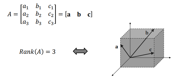
4.4 Proof of the Rank Theorem
Applying these rank rules to our observation equation $W = M \cdot S$:
-
$M$ is a $2F \times 3$ matrix. Hence:
$$\text{Rank}(M) \leq \min(2F, 3) = 3$$
-
$S$ is a $3 \times N$ matrix. Hence:
$$\text{Rank}(S) \leq \min(3, N) = 3$$
-
Applying the product rank theorem:
$$\text{Rank}(W) \leq \min(\text{Rank}(M), \text{Rank}(S)) \leq 3$$
The Tomasi-Kanade Rank Theorem (1992): Under orthographic projection and in the absence of noise, the $2F \times N$ Observation Matrix $W$ has a rank of AT MOST 3, regardless of how many frames $F$ are recorded or how many points $N$ are tracked.
$$\text{Rank}(W) \leq 3$$
This theorem is of paramount importance: even if $W$ contains millions of measurements ($2F \times N$), all data points lie strictly within a 3D subspace. Any non-zero singular values beyond rank 3 are solely due to measurement and tracking noise.
5. The Tomasi-Kanade Factorization Algorithm
Using the Rank Theorem, we can decompose $W$ into $M$ and $S$ using Singular Value Decomposition (SVD).
5.1 Singular Value Decomposition (SVD)
Any $2F \times N$ matrix $W$ can be factored via SVD into:
$$W = U \cdot \Sigma \cdot V^T$$
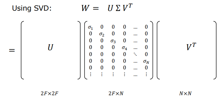
Where:
- $U \in \mathbb{R}^{2F \times 2F}$ contains orthonormal left singular vectors ($U^T U = I$).
- $V^T \in \mathbb{R}^{N \times N}$ contains orthonormal right singular vectors ($V^T V = I$).
- $\Sigma \in \mathbb{R}^{2F \times N}$ contains non-negative singular values sorted in descending order: $\sigma_1 \geq \sigma_2 \geq \sigma_3 \geq \sigma_4 \geq \dots \geq 0$.
5.2 Rank-3 Truncation and Economical Representation
In an ideal noise-free scenario, $\text{Rank}(W) \le 3$, meaning all singular values beyond $\sigma_3$ are exactly zero:
$$\sigma_1 \geq \sigma_2 \geq \sigma_3 > 0 \quad \text{and} \quad \sigma_4 = \sigma_5 = \dots = 0$$
In real-world data, tracking noise causes $\sigma_4, \sigma_5, \dots$ to be small positive values. By the Eckart-Young-Mirsky Theorem, setting $\sigma_i = 0$ for all $i > 3$ yields the optimal rank-3 approximation in the Frobenius norm sense:
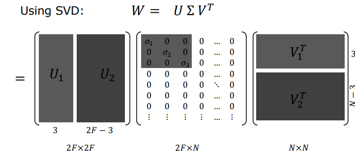
Partitioning into submatrices:
- $U = \begin{bmatrix} U_1 & U_2 \end{bmatrix}$ where $U_1$ is $2F \times 3$.
- $\Sigma = \begin{bmatrix} \Sigma_1 & 0 \\ 0 & \Sigma_2 \end{bmatrix}$ where $\Sigma_1 = \text{diag}(\sigma_1, \sigma_2, \sigma_3)$ is $3 \times 3$.
- $V^T = \begin{bmatrix} V_1^T \\ V_2^T \end{bmatrix}$ where $V_1^T$ is $3 \times N$.
Truncating noise blocks yields the Economical SVD Representation:
$$W \approx U_1 \cdot \Sigma_1 \cdot V_1^T$$
5.3 Factorization and Affine Ambiguity
Since $\Sigma_1$ is positive diagonal, its square root $\Sigma_1^{1/2} = \text{diag}(\sqrt{\sigma_1}, \sqrt{\sigma_2}, \sqrt{\sigma_3})$ is well-defined. Distributing $\Sigma_1^{1/2}$ symmetrically:
$$\hat{M} = U_1 \Sigma_1^{1/2} \quad (2F \times 3) \quad \text{and} \quad \hat{S} = \Sigma_1^{1/2} V_1^T \quad (3 \times N)$$
Thus, $W \approx \hat{M} \cdot \hat{S}$.
However, this solution suffers from Affine Ambiguity: for any invertible $3 \times 3$ matrix $Q$, inserting $Q Q^{-1} = I$ preserves the equality:
$$W = \hat{M} \hat{S} = \left( \hat{M} Q \right) \left( Q^{-1} \hat{S} \right) = M \cdot S$$
Therefore, $\hat{M}$ and $\hat{S}$ are merely affine-distorted versions of the true physical motion and metric structure:
$$M = \hat{M} Q \quad \text{and} \quad S = Q^{-1} \hat{S}$$
To recover true Euclidean metric motion and 3D structure, we must compute the unique $3 \times 3$ transformation matrix $Q$.
5.4 Metric Rectification via Orthonormality Constraints
To resolve the 9 unknowns of $Q$, we exploit the physical geometry of the camera sensor: the row vectors $\mathbf{i}_f$ and $\mathbf{j}_f$ must be orthonormal unit vectors.
For every frame $f$, three geometric constraints must strictly hold:
$$\mathbf{i}_f^T \mathbf{i}_f = 1 \quad (\text{Unit length constraint for } \mathbf{i})$$
$$\mathbf{j}_f^T \mathbf{j}_f = 1 \quad (\text{Unit length constraint for } \mathbf{j})$$
$$\mathbf{i}_f^T \mathbf{j}_f = 0 \quad (\text{Orthogonality constraint})$$
Let $\hat{\mathbf{i}}_f^T$ and $\hat{\mathbf{j}}_f^T$ denote the rows of the unrectified motion matrix $\hat{M}$. Since $M = \hat{M} Q$, the true orientation vectors are $\mathbf{i}_f = Q^T \hat{\mathbf{i}}_f$ and $\mathbf{j}_f = Q^T \hat{\mathbf{j}}_f$. Substituting into the orthonormality conditions:
$$\hat{\mathbf{i}}_f^T \left( Q Q^T \right) \hat{\mathbf{i}}_f = 1$$
$$\hat{\mathbf{j}}_f^T \left( Q Q^T \right) \hat{\mathbf{j}}_f = 1$$
$$\hat{\mathbf{i}}_f^T \left( Q Q^T \right) \hat{\mathbf{j}}_f = 0$$
The unknown to be solved is the symmetric matrix $L = Q Q^T$:
$$L = Q Q^T = \begin{bmatrix} l_1 & l_2 & l_3 \\ l_2 & l_4 & l_5 \\ l_3 & l_5 & l_6 \end{bmatrix}_{3 \times 3}$$
- $L$ is symmetric positive-definite and contains only 6 independent unknowns.
- Each frame provides 3 linear equations.
- For $F \geq 3$ frames, we obtain $3F \geq 9$ equations, forming an overdetermined linear system solvable via Linear Least Squares.
Once $L$ is computed, we extract $Q$ using Cholesky Decomposition or SVD:
$$L = U_L \Sigma_L U_L^T \implies Q = U_L \Sigma_L^{1/2}$$
Finally, the metric camera motion $M$ and metric 3D scene structure $S$ are recovered:
$$\mathbf{M} = \hat{M} Q \quad \text{and} \quad \mathbf{S} = Q^{-1} \hat{S}$$
5.5 Experimental Validation: Classic Tomasi-Kanade Results
In their original 1992 experiments, Tomasi and Kanade validated the algorithm on a toy house model rotated on a turntable.
The reconstructed 3D point cloud showed sub-millimeter geometric accuracy and reconstructed clean perpendicular building walls without any prior calibration.
6. Algorithmic Comparison Matrix
| Algorithmic Step | Mathematical Structure | Purpose / Role | Core Strength / Advantage | Key Limitation / Challenge |
|---|---|---|---|---|
| Centering Trick | Vector subtraction ($\tilde{u} = u - \bar{u}$) | Eliminates camera translations ($C_f$) | Drastically reduces unknowns and linearizes the system | Requires all points to be tracked continuously across all frames |
| Observation Matrix ($W$) | $2F \times N$ dense data matrix | Stacks all 2D trajectory observations | Unifies motion and structure into a bilinear model $W = M \cdot S$ | Outlier tracks or mismatch errors distort the matrix |
| Rank Theorem | $\text{Rank}(W) \leq 3$ bound | Constrains theoretical information dimension | Provides subspace basis for global noise suppression | Strictly valid only under orthographic (parallel) projection |
| SVD & Rank-3 Truncation | $W \approx U_1 \Sigma_1 V_1^T$ truncation | Projects noisy data onto nearest Rank-3 subspace | Globally optimal least-squares denoising (Eckart-Young) | Weak features may be suppressed by singular value cutoff |
| Orthonormality Rectification | $3F$ equations for $L = Q Q^T$ | Resolves affine ambiguity to find metric $M, S$ | Guarantees true Euclidean rotation matrices for camera motion | Potential breakdown if $L$ fails to be positive-definite |
7. Results, Dense Reconstruction, and Modern SfM Extensions
7.1 Dense 3D Surface Reconstruction
While basic factorization produces a sparse point cloud, triangulating tracked features (e.g., Delaunay triangulation) and projecting image intensities via texture mapping yields photorealistic 3D models:
7.2 Modern Extensions: Projective Factorization and Visual SLAM
The Tomasi-Kanade framework inspired several modern paradigms:
- Projective Factorization: Algorithms by Sturm & Triggs and Hartley extended factorization to perspective cameras by iteratively estimating projective depth weights.
- Handling Occlusions (Matrix Completion): Real-world video contains features that enter and exit the frame. Modern methods use low-rank matrix completion and Expectation-Maximization (EM) to handle missing data.
- Internet-Scale SfM: Pipelines like COLMAP and Bundler combine multi-view geometry, pairwise epipolar verification, and non-linear Bundle Adjustment to reconstruct entire cities from unorganized photo collections.
8. Summary of Key Concepts
- Simultaneous Estimation: SfM simultaneously recovers 3D scene structure ($S$) and 3D camera trajectory ($M$) from an uncalibrated video stream without active depth sensors.
- Centering Trick: Translating the world origin to the 3D centroid of scene points eliminates camera translations ($C_f$), yielding the clean linear form $W = M \cdot S$.
- Rank Theorem: Under orthography, the $2F \times N$ observation matrix has rank at most 3 ($\text{Rank}(W) \leq 3$).
- SVD Denoising: SVD truncates singular values beyond rank 3, suppressing measurement noise via optimal low-rank projection ($W \approx U_1 \Sigma_1 V_1^T$).
- Metric Rectification: The affine ambiguity is resolved by enforcing camera orthonormality ($\mathbf{i}_f^T \mathbf{i}_f = 1, \mathbf{j}_f^T \mathbf{j}_f = 1, \mathbf{i}_f^T \mathbf{j}_f = 0$), solving $L = Q Q^T$ linearly to recover the true metric reconstruction.
Object Tracking & Background Subtraction
- 1. Overview
- 2. Change Detection
- 3. Gaussian Mixture Model (GMM)
- 3.1 Multimodal Nature of Pixel Temporal Distributions
- 3.2 Mathematical GMM Formulation (1D Case)
- 3.3 Multidimensional GMM in Color Space (RGB & Covariance Matrices)
- 3.4 Classification Rule: Foreground vs. Background ($\omega / \sigma$ Ratio)
- 3.5 Online Adaptive GMM Algorithm (Stauffer-Grimson)
- 3.6 Performance Comparison: GMM vs. Moving Median
- 4. Object Tracking using Template Matching
- 5. Tracking by Feature Detection
- 6. Technical Summary & Comparison Matrix
This lecture note comprehensively covers Object Tracking and Change Detection / Background Subtraction, two fundamental pillars of dynamic scene analysis and perception in computer vision. Beginning with pixel-level differential motion analysis, it explores statistical and probabilistic Gaussian Mixture Models (GMM), local template and histogram-based tracking methods, and robust SIFT-based “Bag of Features” tracking architectures following the curriculum of Columbia University’s CAVE Laboratory (Prof. Shree K. Nayar).
1. Overview
In computer vision, Object Tracking is the process of continuously, robustly, and automatically estimating the spatial position, geometric boundaries, scale, and trajectory of a specific target object or Region of Interest (ROI) across temporally sequential video frames ($I_1, I_2, \dots, I_T$).
While Optical Flow solves for where every individual pixel moves between consecutive frames at a differential level (dense/sparse vector motion field $\mathbf{u} = [u, v]^T$), object tracking aims to track a coherent holistic entity (e.g., a person, vehicle, face, or athlete) as a semantic whole rather than treating pixels independently.
flowchart LR
subgraph OpticalFlow["Optical Flow"]
OF1["Pixel-Level Differential Analysis"] --> OF2["Local Motion Vectors (u, v)"]
end
subgraph ObjectTracking["Object Tracking"]
OT1["Holistic / Regional Entity Representation"] --> OT2["ROI / Bounding Box Trajectory Estimation"]
end
style OpticalFlow fill:#1a1a2e,stroke:#e94560,color:#fff
style ObjectTracking fill:#16213e,stroke:#4cc9f0,color:#fff
1.1 Fundamental Challenges in Object Tracking
In real-world operating environments, tracking algorithms must remain resilient against severe optical, physical, and environmental disturbances:
- Illumination Changes: Sudden changes in pixel intensity and color caused by clouds obscuring the sun, flickering artificial lights, or an object entering shadow cast by buildings or trees.
- Scale Changes: Continuous expansion or shrinkage of the target’s image resolution and bounding box footprint as it moves toward or away from the camera.
- Rotation & Viewpoint Changes: Drastic 2D appearance variations caused by out-of-plane 3D rotations of the object (e.g., a car navigating a turn or a person turning their head).
- Occlusions: Partial or full visual disappearance of the tracked target when passing behind static obstacles (poles, trees, traffic signs) or dynamic objects (other pedestrians or cars).
- Camera Shake & Dynamic Backgrounds: Mechanical vibrations and wind-induced camera motion, alongside periodic scene motions such as swaying foliage, rippling water surfaces, or passing precipitation.
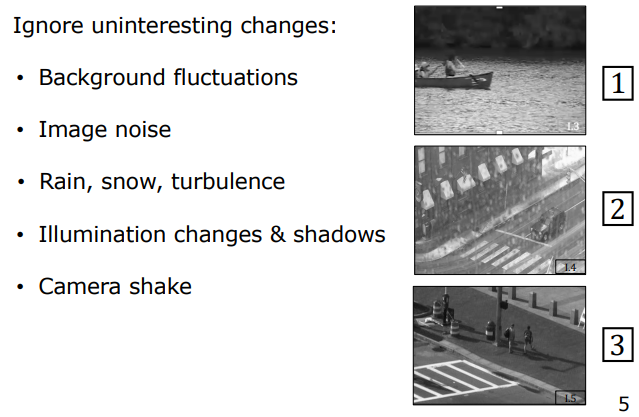
1.2 The Two Primary Stages of Object Tracking
A modular modern visual tracking system is organized into two complementary stages:
- Change Detection (Background Subtraction): Segmenting temporally moving or novel pixels from the static background (Foreground / Background Classification).
- Motion Tracking and Localization: Continuously estimating the object’s updated bounding box in subsequent frames using appearance templates, color histograms, or local feature matchers.
flowchart TD
subgraph Stage1["Stage 1: Change Detection"]
A["Video Stream (I_t)"] --> B["Background Modeling (GMM / Median)"]
B --> C["Foreground Mask"]
end
subgraph Stage2["Stage 2: Tracking & Localization"]
C --> D["Target Initialization (ROI / Bounding Box)"]
D --> E["Template / Histogram / SIFT Matching"]
E --> F["Optimal New Location (W_t) & Model Update"]
end
style Stage1 fill:#1a1a2e,stroke:#e94560,color:#fff
style Stage2 fill:#16213e,stroke:#4cc9f0,color:#fff
2. Change Detection
To initialize or support tracking autonomously in stationary cameras, the system must detect where “meaningful motion” occurs in the scene.
2.1 Foreground vs. Background Classification Problem
Change detection formulates a real-time binary decision for each pixel coordinate $(x, y)$:
- Foreground (FG): Meaningful dynamic objects of interest (e.g., walking pedestrians, moving vehicles).
- Background (BG): Static or repetitive structural components of the scene (roads, buildings, walls, ground).
The core challenge is distinguishing meaningful changes from uninteresting (irrelevant) fluctuations:
- Background Fluctuations: Swaying branches, rustling leaves, or specular highlights on moving water.
- Sensor Noise: Random thermal and quantum photon shot noise, particularly prominent in low-light imagery.
- Weather Effects: Rapidly transient raindrops, falling snowflakes, or atmospheric heat mirages (turbulence).
- Moving Shadows: Dark regions cast on the ground that move coherently with the target but are not physically part of the object geometry.
- Camera Jitter: Sub-pixel to multi-pixel rigid translations caused by wind or platform vibrations.
2.2 Methods and Evolution of Change Detection
The historical development of change detection has progressed from simple deterministic frame differencing to adaptive probabilistic distributions.
2.2.1 Frame Differencing
The simplest baseline method computes the absolute intensity difference between the current frame ($I_t$) and the immediately preceding frame ($I_{t-1}$), thresholding the result by a constant $\tau$:
$$F(x, y, t) = \begin{cases} 1 & \text{if } |I(x, y, t) - I(x, y, t-1)| > \tau \ 0 & \text{otherwise} \end{cases}$$
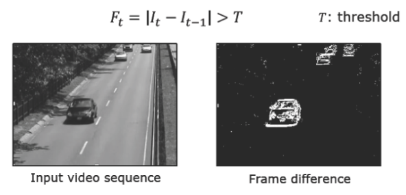
Critical Drawbacks (The “Hole” Problem):
- Any minor leaf flutter or sensor noise immediately generates false foreground positives.
- Interior Cavities (Holes): If a moving object (e.g., a solid gray car) has a uniform interior surface, the intensity at interior pixels does not change between adjacent frames ($|I_t - I_{t-1}| \approx 0$). Consequently, the detected mask is hollow, showing only leading and trailing edges, making holistic tracking and sizing unreliable.
2.2.2 Average Background Method
To overcome the interior hole problem of frame differencing, a single Reference Background Image ($B$) is computed by averaging the first $K$ video frames:
$$B(x, y) = \frac{1}{K} \sum_{i=1}^K I(x, y, i)$$
Subsequent frames are compared directly against this static background:
$$F(x, y, t) = |I(x, y, t) - B(x, y)| > \tau$$
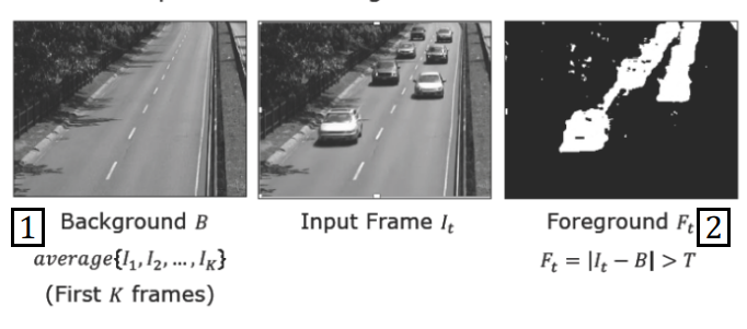
Drawbacks:
- If any foreground object moves through the scene during the initial $K$ frames, it gets permanently etched as a “ghost” artifact into the reference model.
- The model is static; it cannot adapt to gradual changes in sunlight, cloud cover, or moving shadows, eventually classifying the entire scene as foreground.
2.2.3 Median Background Method
Rather than computing the arithmetic mean, the statistical median of pixel values across the first $K$ frames is selected as the background model:
$$B(x, y) = \text{median}{I(x, y, 1), I(x, y, 2), \dots, I(x, y, K)}$$
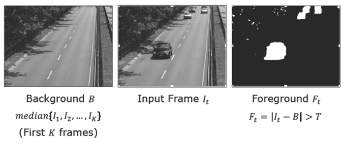
Strength of the Median: The median operator is inherently robust against transient outliers. Even if cars pass through a pixel location during training, their transient values occupy the distribution extremes and do not distort the median. However, the static median still fails when the physical environment evolves over time.
2.2.4 Adaptive / Moving Median Method
To track gradual lighting changes, the median model is updated recursively across a sliding temporal window or via an incremental step rule:
$$B_t(x, y) = \begin{cases} B_{t-1}(x, y) + 1 & \text{if } I(x, y, t) > B_{t-1}(x, y) \ B_{t-1}(x, y) - 1 & \text{if } I(x, y, t) < B_{t-1}(x, y) \ B_{t-1}(x, y) & \text{otherwise} \end{cases}$$
While effective for slow global lighting drift, the adaptive median maintains only a single scalar intensity per pixel and remains fundamentally unable to model multimodal background distributions (such as rustling leaves or active snowfall).
3. Gaussian Mixture Model (GMM)
In real-world scenes, a pixel’s temporal intensity distribution is often multimodal rather than unimodal. For example, a pixel observing a wind-blown tree branch oscillates between the bright blue sky and the dark green leaves, producing two distinct peaks (a bimodal distribution) in its temporal histogram.
3.1 Multimodal Nature of Pixel Temporal Distributions
Consider an outdoor surveillance camera monitoring a roadway during heavy snowfall. Observing a single pixel over hundreds of frames reveals a distinct multimodal histogram:
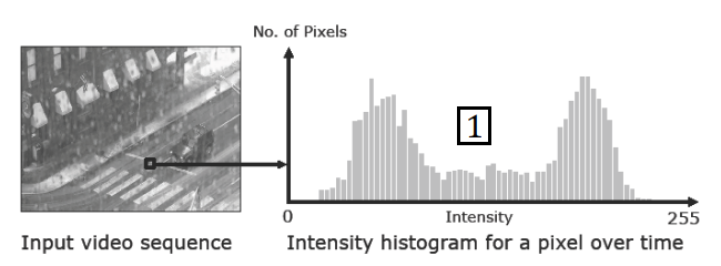
Physical decomposition of this temporal distribution reveals three distinct components:
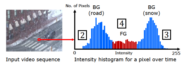
- Static Background (Road/Asphalt): Highly frequent, narrow variance peak representing the persistent surface.
- Dynamic Background (Falling Snow): Frequently recurring, broader variance peak representing repetitive weather disturbance.
- Foreground Objects (Vehicles): Rare, transient occurrences with very low supporting evidence/weight.
Key GMM Insight: Foreground objects occupy a given pixel location only rarely. Background and repetitive disturbance states dominate the temporal history of the pixel.
3.2 Mathematical GMM Formulation (1D Case)
GMM models the probability density of a pixel intensity $x$ as a weighted mixture of $K$ independent Gaussian distributions ($K = 3, 4, 5$):
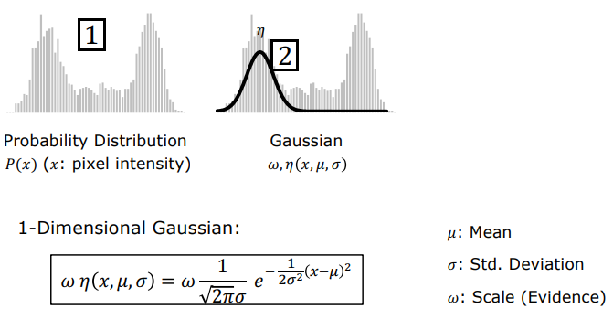
For grayscale imagery, the probability density function is:
$$P(x) = \sum_{k=1}^K \omega_k \cdot \eta(x \mid \mu_k, \sigma_k^2)$$
where:
$$\eta(x \mid \mu_k, \sigma_k^2) = \frac{1}{\sqrt{2\pi}\sigma_k} e^{-\frac{(x - \mu_k)^2}{2\sigma_k^2}}$$
- $\mu_k$ : Mean intensity of the $k$-th Gaussian component (peak center).
- $\sigma_k$ : Standard deviation of the $k$-th component (peak width / variance).
- $\omega_k$ : Weight / Evidence coefficient representing the proportion of time the pixel exhibits this state.
The mixture weights are normalized:
$$\sum_{k=1}^K \omega_k = 1$$
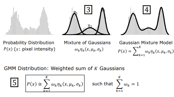
3.3 Multidimensional GMM in Color Space (RGB & Covariance Matrices)
In 3D color space ($\mathbf{x} = [R, G, B]^T, d=3$), the multivariate Gaussian formulation is:
$$P(\mathbf{x}) = \sum_{k=1}^K \omega_k \cdot \frac{1}{(2\pi)^{d/2} |\Sigma_k|^{1/2}} e^{-\frac{1}{2}(\mathbf{x} - \boldsymbol{\mu}_k)^T \Sigma_k^{-1} (\mathbf{x} - \boldsymbol{\mu}_k)}$$
- $\boldsymbol{\mu}_k = [\mu_R, \mu_G, \mu_B]^T$ : $3 \times 1$ mean color vector.
- $\Sigma_k$ : $3 \times 3$ covariance matrix.
| Covariance Model | Matrix Structure | Geometric Shape | Computation Speed | Fidelity |
|---|---|---|---|---|
| Isotropic / Spherical | $\Sigma_k = \sigma_k^2 I$ | Sphere in 3D RGB space | Very Fast | Baseline |
| Diagonal | $\Sigma_k = \text{diag}(\sigma_R^2, \sigma_G^2, \sigma_B^2)$ | Axis-aligned ellipsoid | Fast | Good |
| Full Covariance | $\Sigma_k = \begin{bmatrix} \sigma_{RR} & \sigma_{RG} & \sigma_{RB} \ \sigma_{GR} & \sigma_{GG} & \sigma_{GB} \ \sigma_{BR} & \sigma_{BG} & \sigma_{BB} \end{bmatrix}$ | Rotated 3D ellipsoid | Computationally Heavy | Highest |
3.4 Classification Rule: Foreground vs. Background ($\omega / \sigma$ Ratio)
To determine which of the $K$ Gaussians represent background states and which represent foreground anomalies, the components are sorted by their fitness score:
$$\text{Component Score} = \frac{\omega_k}{\sigma_k}$$
- Background Gaussians (High $\omega_k / \sigma_k$): Persistent presence (large $\omega_k$) and low noise variance (small $\sigma_k$). The top $B$ ranked Gaussians accounting for a cumulative weight threshold $T$ are designated as the background model.
- Foreground Gaussians (Low $\omega_k / \sigma_k$): Transient presence (small $\omega_k$) and motion blur / variability (large $\sigma_k$).
3.5 Online Adaptive GMM Algorithm (Stauffer-Grimson)
Fitting a full EM algorithm at every pixel in real-time is computationally intractable. Stauffer and Grimson (1999) introduced an efficient online recursive update scheme:
flowchart TD
Start["New Video Frame I_t(x, y)"] --> Match["Find Nearest Gaussian (|x - \mu_k| < 2.5 \sigma_k)"]
Match -- "Matched" --> UpdateMatched["Update Matched Component:\n\omega_k ↑, \mu_k and \sigma_k shift toward new value"]
Match -- "Unmatched" --> ReplaceLowest["Replace Lowest Weight Component with New Gaussian"]
UpdateMatched --> CheckScore["Evaluate \omega_k / \sigma_k Rank"]
ReplaceLowest --> CheckScore
CheckScore -- "Ranked as BG" --> BG["Background"]
CheckScore -- "Ranked as FG" --> FG["Foreground (Meaningful Motion)"]
style Start fill:#1a1a2e,stroke:#e94560,color:#fff
style Match fill:#16213e,stroke:#4cc9f0,color:#fff
style UpdateMatched fill:#0f3460,stroke:#4cc9f0,color:#fff
style ReplaceLowest fill:#0f3460,stroke:#e94560,color:#fff
style BG fill:#1b262c,stroke:#00b4d8,color:#fff
style FG fill:#2c1b1b,stroke:#ff6b6b,color:#fff
- Mahalanobis Matching Test: The incoming intensity $x_t$ is checked against each component. A match occurs if $x_t$ falls within $2.5$ standard deviations of $\mu_k$: $$|x_t - \mu_k| \le 2.5 \sigma_k$$
- Recursive Parameter Updates:
- For the matched component: $\omega_k \leftarrow (1-\alpha)\omega_k + \alpha$
- Mean shifts: $\mu_k \leftarrow (1-\rho)\mu_k + \rho x_t$
- Variance shifts: $\sigma_k^2 \leftarrow (1-\rho)\sigma_k^2 + \rho (x_t - \mu_k)^2$
- Unmatched components decay: $\omega_j \leftarrow (1-\alpha)\omega_j$
- Handling Unmatched Pixels: If no Gaussian matches $x_t$, the component with the lowest $\omega/\sigma$ is replaced with a new Gaussian centered at $x_t$ with high initial variance and low weight.
3.6 Performance Comparison: GMM vs. Moving Median
4. Object Tracking using Template Matching
Once a target is localized (via change detection or user initialization), Template Matching tracks the object across subsequent video frames by searching for matching image regions.
Template matching relies on two primary target representation paradigms:
4.1 Appearance-Based Tracking
- Mechanism: The raw 2D pixel array within the bounding box is saved as an Image Template ($T$). In the next frame $I_t$, this template is shifted across a local search window centered around the target’s prior position.
- Similarity Metrics:
- SAD (Sum of Absolute Differences): $\text{SAD}(u, v) = \sum_{x, y} |I(x+u, y+v) - T(x, y)|$
- SSD (Sum of Squared Differences): $\text{SSD}(u, v) = \sum_{x, y} (I(x+u, y+v) - T(x, y))^2$
- NCC (Normalized Cross-Correlation): Illuminance-invariant normalized dot product.
- Limitations: Highly sensitive to target rotation, scale changes, non-rigid deformations, and occlusions, causing tracking failure under geometric transformations.
4.2 Histogram-Based Tracking
- Mechanism: Represents the target as a color or intensity histogram rather than a rigid spatial pixel matrix.
- Strengths: By discarding spatial pixel coordinates, histograms are inherently invariant to 2D in-plane and 3D out-of-plane rotations and flexible body deformations.
- Vulnerability (Background Clutter Contamination): Rectangular bounding boxes inevitably enclose background pixels at their corners (e.g., grass, road). As the target moves, these extraneous pixels pollute the histogram, causing the tracker to drift into the background.
4.3 Spatial Weighting with the Epanechnikov Kernel
To suppress background contamination at bounding box corners, an isotropic Epanechnikov Kernel is applied to weight pixel contributions according to their distance from the ROI center:
For a window of size $(2W+1) \times (2H+1)$ centered at $\mathbf{x}_c = [x_c, y_c]^T$, normalized coordinates are:
$$\mathbf{\tilde{x}} = \begin{bmatrix} \frac{x - x_c}{W} \ \frac{y - y_c}{H} \end{bmatrix}$$
The parabolic Epanechnikov kernel profile is:
$$k(\mathbf{\tilde{x}}) = \begin{cases} 1 - |\mathbf{\tilde{x}}|^2 & \text{if } |\mathbf{\tilde{x}}| < 1 \ 0 & \text{otherwise} \end{cases}$$
4.4 Histogram Intersection and the Latching Problem
To compare two normalized histograms ($H_1$ and $H_2$), the standard Histogram Intersection metric is used:
$$D(H_1, H_2) = \sum_{i=1}^M \min(H_1(i), H_2(i))$$
- Occlusion Robustness: Because of the minimum operator ($\min$), partial occlusions only reduce the score proportionally to the obscured area without causing tracking collapse.
- Latching / Identity Switch Failure Mode: Since histograms discard all spatial arrangement, if the target (e.g., a basketball player in a red jersey) passes closely beside a teammate wearing the same uniform, the tracker cannot disambiguate them and frequently locks onto the wrong player (latching / identity switch).
5. Tracking by Feature Detection
To overcome the rigid alignment limits of template matching and the spatial ambiguity of histograms, SIFT-Based “Bag of Features” Tracking (Gu et al., 2010) models the target as an ensemble of distinctive local invariant features.
5.1 Initialization and Bag of Features Construction
At the initial video frame ($t=1$):
- Bounding Box Placement: A bounding box $W_1$ is positioned over the target.
- Feature Extraction: SIFT detector runs across the entire frame, generating 128-dimensional descriptor vectors ($\mathbf{v}_i$).
- Object Model ($O_1$ Bag): Keypoints falling inside $W_1$ are stored in the Object Bag ($O_1$) (Blue points).
- Background Model ($B$ Bag): All keypoints falling outside $W_1$ are stored in the Background Bag ($B$) (Red points).
5.2 Frame-to-Frame Tracking & Confidence Ratio Test
In each subsequent frame $I_t$:
-
Feature Extraction: SIFT detects a new set of candidate features ${\mathbf{v}_1, \dots, \mathbf{v}_K}$ in frame $I_t$.
-
Nearest-Neighbor Distance Ratio Test: For each feature $\mathbf{v}_i$:
- Distance to nearest match in Object Bag ($O_{t-1}$): $d_O = \min_{\mathbf{u} \in O_{t-1}} |\mathbf{v}_i - \mathbf{u}|$
- Distance to nearest match in Background Bag ($B$): $d_B = \min_{\mathbf{u} \in B} |\mathbf{v}_i - \mathbf{u}|$
Confidence score assignment:
$$C(\mathbf{v}_i) = \begin{cases} +1 & \text{if } \frac{d_O}{d_B} < 0.5 \quad (\mathbf{v}_i \text{ belongs to target object}) \ -1 & \text{otherwise } (\mathbf{v}_i \text{ belongs to background}) \end{cases}$$
5.3 Optimal Window Search and Geometric Penalty
Candidate search windows ($W$) are evaluated by translating and scaling around $W_{t-1}$. The tracking objective function is:
$$\mu(W) = \varphi(W) - \tau(W, W_{t-1})$$
- Window Feature Score: $\varphi(W) = \sum_{\mathbf{v}_i \in W} C(\mathbf{v}_i)$ (Maximizes inclusion of $+1$ object features while penalizing $-1$ background features).
- Geometric Shape Penalty: $\tau(W, W_{t-1})$ penalizes large, abrupt deviations in position, aspect ratio, and scale relative to $W_{t-1}$.
The optimal location is chosen by maximizing $\mu(W)$:
$$W_t = \arg\max_W \mu(W)$$
5.4 Online Appearance Model Update
To prevent model drift and adapt to perspective shifts, verified object features in $W_t$ are dynamically appended to the object bag:
$$O_t = O_{t-1} \cup {\mathbf{v}_i \mid \mathbf{v}_i \in W_t \text{ and } C(\mathbf{v}_i) = +1}$$
5.5 Robustness to Occlusion, Rotation, and Lighting
- Occlusion Resistance: When an obstacle (e.g., a hat or magazine) partially occludes the target, new obstacle features fail the ratio test ($C = -1$), preventing window deformation. The remaining unoccluded SIFT keypoints ($C = +1$) keep the tracking window locked onto the target.
- 3D Rotation & Illumination Invariance: SIFT descriptors provide scale, rotational, and gradient contrast invariance, maintaining tracking throughout complex 3D maneuvers.
6. Technical Summary & Comparison Matrix
| Method | Core Decision Metric / Formula | Required Input Data | Key Strengths | Primary Failure Mode |
|---|---|---|---|---|
| Frame Differencing | $\lvert I_t - I_{t-1} \rvert > \tau$ | Adjacent frame pair | Extremely fast, simple change detector | Hollow interior holes on uniform objects; sensitive to leaves/noise |
| Median Background | $\lvert I_t - \text{median}{I_1, \dots, I_K} \rvert > \tau$ | First $K$ video frames | Highly robust against transient outliers during training | Static model; cannot handle ambient diurnal illumination changes |
| Gaussian Mixture Model (GMM) | $\frac{\omega_k}{\sigma_k}$ ranking + Mahalanobis test | $K$ Gaussian parameters $(\omega_k, \mu_k, \Sigma_k)$ per pixel | Multimodal backgrounds (snow, rain, swaying trees, camera jitter) | Cannot separate dark moving cast shadows sharing target chromaticity |
| Appearance Template | $\min \text{SSD}$ or $\max \text{NCC}$ | Initial raw pixel matrix | Short-term linear translational tracking | Scale change, 3D rotation, or occlusion causes immediate tracking loss |
| Weighted Histogram | Epanechnikov weighted histogram intersection | Weighted color distribution of ROI | Invariant to rotation and non-rigid deformations | Ambiguity when crossing identically colored targets (latching / identity switch) |
| Bag of Features (SIFT) | $\max (\varphi(W) - \tau(W))$ with SIFT ratio test | Object ($O$) and Background ($B$) SIFT feature bags | Severe occlusions, 3D rotations, complex lighting | Completely textureless, featureless objects lacking SIFT keypoints |
Image Segmentation Foundations and Clustering Mathematics
- 1. Overview and Segmentation Strategies
- 2. Segmentation by Humans (Gestalt Psychology)
- 3. Segmentation as Clustering Mathematics
- 4. k-Means Segmentation
- 5. Mean-Shift Segmentation
- 6. Graph-Based Segmentation
- 7. Summary Comparison Matrix
This note covers Image Segmentation, one of the fundamental and inherently “ill-defined” problems in computer vision; starting from human visual physiology and Gestalt perceptual grouping laws, to clustering in pixel feature space, k-Means and Mean-Shift algorithms, and spectral graph theory with Normalized Cuts (NCut), following the curriculum of Columbia University’s CAVE lab (Prof. Shree K. Nayar).
1. Overview and Segmentation Strategies
Image Segmentation is the process of partitioning a digital image into multiple visually, geometrically, or semantically coherent, homogeneous, and meaningful regions (segments). It serves as a critical precursor step for higher-level computer vision tasks such as object detection, object recognition, 3D scene understanding, and image classification.
1.1 Primitive Segmentation Approaches
Before establishing the general theory of segmentation, two classic, primitive approaches frequently used in early computer vision are:
- Histogram Thresholding: In simple scenarios where an object rests on a homogeneous, distinct background, the image intensity histogram is computed. By finding the valley between two major peaks in the histogram, a threshold $T$ is selected, and pixels are converted into a binary mask according to $I(x,y) > T$.
- Active Contours (Snakes): An approximate initial closed contour is placed around the object. Under the influence of internal elastic tension/bending forces and external image forces (intensity gradients), the contour automatically expands or contracts to snap (latch) onto the object’s true boundary. However, because it requires manual initialization, it cannot solve the general, fully automated segmentation problem.

1.2 The “Ill-Defined” and Subjective Nature of Segmentation
When attempting to perform general segmentation on natural scenes, we encounter the fundamental dilemma that there is no unique, absolute mathematical definition of a “meaningful segment.”
- Example Scenario: In a photograph of a person wearing a hat, should the hat be segmented together with the person as a single object, or should they be separated into two distinct segments? The answer depends entirely on the downstream task, context, and application.
- Human Subjectivity: In psychophysical experiments conducted by Martin et al. (2001), identical natural images were presented to multiple human subjects who were asked to draw meaningful segments. The results showed that one subject divided the image into coarse regions, another traced architectural and facial details, while a third segmented even fine decorative elements. Segmentation is inherently subjective, even for human observers.
1.3 Two Core Segmentation Paradigms
To formulate algorithmic solutions, two primary paradigms are established:
flowchart TD
Input["Input Natural Image"] --> Split{"Segmentation Paradigm"}
Split --> BU["Bottom-Up Segmentation\n• Local visual feature similarity (color, texture, location)\n• Clustering in feature space\n• No prior object model required"]
Split --> TD["Top-Down Segmentation\n• Global object models and Gestalt templates\n• Detect object first, then segment its components\n• Requires prior knowledge and recognition models"]
style Input fill:#1a1a2e,stroke:#e94560,color:#fff
style Split fill:#16213e,stroke:#4cc9f0,color:#fff
style BU fill:#0f3460,stroke:#4cc9f0,color:#fff
style TD fill:#0f3460,stroke:#e94560,color:#fff
- Top-Down Segmentation: Pixels group together because they belong to the same global object model. The system detects the object first and subsequently segments its parts.
- Bottom-Up Segmentation: Pixels group together because their local visual features (color, brightness, texture, coordinates) are similar. This converts the segmentation task into a well-defined Clustering problem in Feature Space.
2. Segmentation by Humans (Gestalt Psychology)
The most influential psychological framework explaining how the human visual system effortlessly groups and segments complex scenes in milliseconds is Gestalt Psychology (German for “form / shape / unified whole”). Its foundational principle states that we perceive objects in their entirety before their individual parts, subsequently identifying sub-elements.
Dalmatian Dog Experiment: When looking at an abstract collection of black-and-white splotches, our visual system suddenly perceives the whole Dalmatian dog. Only after recognizing the dog as a whole can we distinguish its legs, head, and tail.
Todorovic (2008) and Smith (1988) systematized the core Gestalt grouping principles:
2.1 Principle of Proximity
Objects and elements that are spatially closer to one another are automatically grouped together by our visual system. While uniformly spaced dots form a single uniform field, altering the relative distance creates distinct sub-clusters.
2.2 Principle of Similarity
Visual elements that share similar appearance features (brightness, color, scale, orientation) are grouped together.
- Competition: When similarity and proximity compete (e.g., pairs of different colored dots placed very close together), proximity usually dominates, leading us to perceive the closely positioned pairs as units despite differing colors.
2.3 Principle of Common Fate
Even if visual elements are spatially separated, elements that move in the same direction and at the same velocity (sharing a “common fate”) or undergo synchronous appearance changes are immediately unified into a single group.
2.4 Principle of Common Region and Connectedness
Elements enclosed within bounded regions (ellipses/boxes) or physically linked by connecting lines are perceived as unified sub-groups, overriding uniform spatial proximity.
2.5 Principle of Continuity
Visual features lying on a smooth, continuous geometric curve are perceived as a single coherent trajectory, even across intersections and gaps.
2.6 Principle of Symmetry
Parallel and symmetrical structures (translation or reflection symmetry) produce strong grouping cues. In the physical world, unrelated objects forming accidental symmetry is extremely unlikely; thus, symmetrical structures are strongly bound together by human perception.
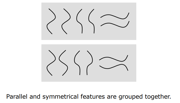
3. Segmentation as Clustering Mathematics
In the bottom-up paradigm, each pixel in an image is represented by a high-dimensional Feature Vector ($\mathbf{f}_i$) constructed from measurable and computable visual properties.
3.1 Pixel Feature Space
The feature vector $\mathbf{f}_i$ can incorporate:
- Measurable Properties: Pixel intensity ($I$), color channels ($R, G, B$).
- Spatial Coordinates: Image plane coordinates ($x, y$).
- Computable Properties: Depth ($z$ / $d$) from stereo/ToF/defocus; optical flow motion vectors ($u, v$); local texture descriptors and BRDF reflectance parameters.
$$\mathbf{f}_i = \begin{bmatrix} R \ G \ B \ x \ y \ d \ \vdots \end{bmatrix}$$
This vector maps each pixel as a discrete point in a high-dimensional Euclidean Space ($n$-space).
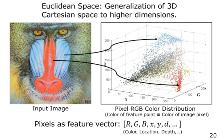
3.2 Pixel Similarity and Euclidean Distance
To mathematically quantify visual similarity between two pixels ($i$ and $j$), the $\mathcal{L}_2$ (Euclidean) distance between their feature representations ($\mathbf{f}_i$ and $\mathbf{f}_j$) is computed:
$$\mathcal{L}_2(\mathbf{f}_i, \mathbf{f}_j) = |\mathbf{f}_i - \mathbf{f}_j| = \sqrt{\sum_{k=1}^D (f_{ik} - f_{jk})^2}$$
According to this metric: the smaller the distance in feature space, the greater the visual and spatial similarity between the pixels. Image segmentation thus reduces to running Clustering algorithms in this feature space.
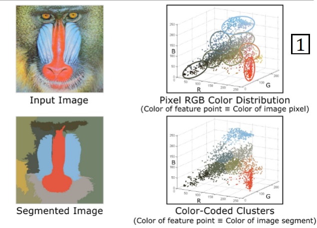
4. k-Means Segmentation
k-Means is one of the most widely used, straightforward, and efficient clustering algorithms in computer vision, based on Lloyd’s algorithm.
4.1 Algorithm Steps
To obtain $k$ segments from an $N$-pixel image:
flowchart TD
Init["Step 1: Initialization\nRandomly select k initial centroids: {m_1, m_2, ..., m_k}"] --> Assign["Step 2: Pixel Assignment\nAssign each pixel to its nearest centroid:\nCluster(x_j) = argmin_i ||f_j - m_i||"]
Assign --> Update["Step 3: Centroid Update\nRecompute means of all assigned pixels:\nm_i = (1 / N_i) ∑ f_j"]
Update --> Check{"Step 4: Convergence Check\n||Δm_i|| < ε ?"}
Check -- "No" --> Assign
Check -- "Yes" --> Done["Segmentation Complete\nAssign unique label/color to each cluster"]
style Init fill:#1a1a2e,stroke:#e94560,color:#fff
style Assign fill:#16213e,stroke:#4cc9f0,color:#fff
style Update fill:#0f3460,stroke:#4cc9f0,color:#fff
style Check fill:#1b262c,stroke:#f9bc60,color:#fff
style Done fill:#0f4c5c,stroke:#00b4d8,color:#fff
- Initialization: Randomly pick $k$ cluster centers (means) in feature space: ${m_1, m_2, \dots, m_k}$.
- Assignment: For each pixel $x_j$, find the closest mean $m_i$ and assign the pixel to cluster $i$: $$\text{Assign}(x_j) = \arg\min_{i} |\mathbf{f}_j - m_i|$$
- Centroid Update: Recalculate each cluster’s mean as the arithmetic average of all pixels assigned to it: $$m_i = \frac{1}{N_i} \sum_{j \in \text{Cluster } i} \mathbf{f}_j$$
- Convergence Check: If the shift in all $k$ centroids is less than a tolerance $\epsilon$, terminate; otherwise, repeat Step 2.
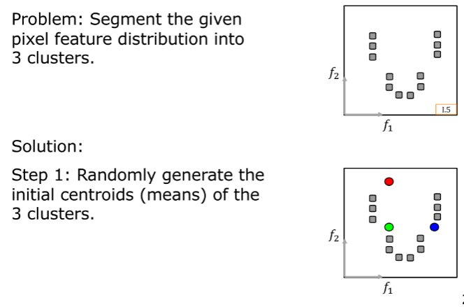
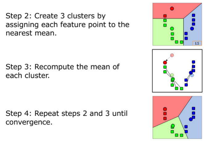
4.2 Centroid Initialization Methods
Because k-Means is susceptible to local minima, initialization is critical:
- Method 1 (Random Selection): Pick $k$ points uniformly at random from data. If two points are too close, resample.
- Method 2 (Uniform Bounding Box): Compute the bounding box of all data in feature space and uniformly distribute $k$ grid centroids across it.
- Method 3 (Subset k-Means - Most Robust): Randomly sample a small subset (e.g., 100 or 1000 pixels), run k-Means on this subset, and use the resulting stable centers as initial centroids for the full image.
4.3 Impact of Cluster Count $k$
The choice of $k$ dictates the granularity of segmentation:
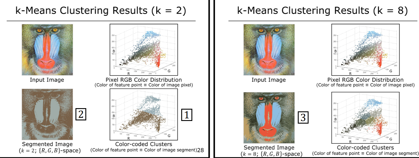
4.4 Spatial Coherence: RGB vs. RGB-XY Space
- Pure Color Space (RGB): Segmenting solely in RGB groups spatially disconnected regions of the same color into the same cluster (disjoint regions). For instance, a pepper and distant leaves with similar green tones share one cluster label.
- Incorporating Spatial Coordinates (RGB-XY): Expanding the feature vector to 5D ($\mathbf{f} = [R, G, B, x, y]^T$) enforces spatial proximity alongside color consistency, producing continuous, compact object segments.
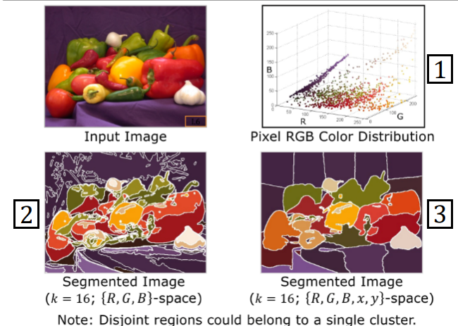
Key Limitations of k-Means:
- Requires pre-specifying the exact number of clusters $k$.
- Highly sensitive to initial centroid placement.
- Vulnerable to outliers, which can distort entire cluster centers.
5. Mean-Shift Segmentation
Mean-Shift is a non-parametric, probabilistic hill-climbing (gradient ascent) algorithm (Comaniciu & Meer, 2002) that overcomes both key drawbacks of k-Means (no need to specify $k$ in advance and immunity to initialization sensitivity).
5.1 Probability Density Peaks and Modes
The distribution of pixels in feature space is modeled as a smooth continuous Probability Density Function (PDF), analogous to a topographic landscape of hills and valleys:
- Each hill represents a distinct cluster (segment).
- The peak (mode) of a hill represents the center of that cluster.
- Each pixel climbs the steepest local gradient within its neighborhood (hill-climbing).
- All pixels that converge to the same mode belong to the same cluster. Consequently, the number of clusters $k$ is discovered organically.
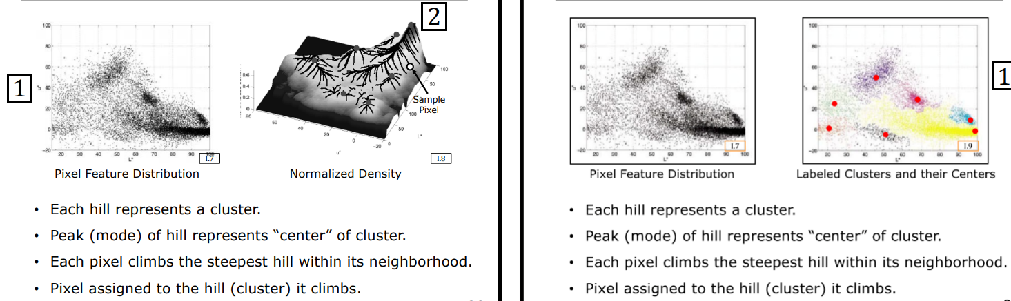
5.2 Mean-Shift Algorithm Steps
Given $N$ points and a circular/spherical analysis window of radius $W$ (bandwidth):
- Set the initial location of pixel $i$ to its feature value: $m_i^{(0)} = \mathbf{f}_i$.
- Place a window of radius $W$ centered at $m_i$.
- Compute the weighted center of mass (centroid) of all data points inside the window: $$m = \frac{\sum_{\mathbf{x}_j \in W(m_i)} K(\mathbf{x}_j - m_i) \mathbf{x}_j}{\sum_{\mathbf{x}_j \in W(m_i)} K(\mathbf{x}_j - m_i)}$$
- Shift the window center to this newly computed centroid ($m_i \leftarrow m$). This displacement vector is the Mean Shift Vector.
- Repeat Steps 2–4 until the shift magnitude falls below $\epsilon$ (the window reaches the peak/mode).
- Assign the converged mode as the cluster center; all pixels climbing to the same mode receive the same segment label.
5.3 Comparison: k-Means vs. Mean-Shift
- Outliers and Non-Convex Shapes: While k-Means assumes spherical clusters and gets easily corrupted by outliers and varying densities (e.g., Mickey Mouse distribution), Mean-Shift cleanly isolates the head and both ears without being skewed by noisy points.
Mean-Shift Trade-offs:
- Pros: Automatic discovery of cluster count, handles arbitrary shapes, robust to outliers.
- Cons: Computationally expensive (hill-climbing performed independently for every pixel), highly sensitive to bandwidth $W$ (too small $\rightarrow$ over-segmentation; too large $\rightarrow$ under-segmentation).
6. Graph-Based Segmentation
Graph-based segmentation models the image not as an isolated set of points in feature space, but as a densely connected relational network (graph).
6.1 Images as Graphs
An image is represented as a weighted undirected graph $G = (V, E)$:
- Vertices ($V$): Each pixel is a vertex/node in the graph.
- Edges ($E$): Connections between neighboring pixel pairs.
- Edge Weights ($w(i,j)$): Affinity (Similarity) between pixels $i$ and $j$.
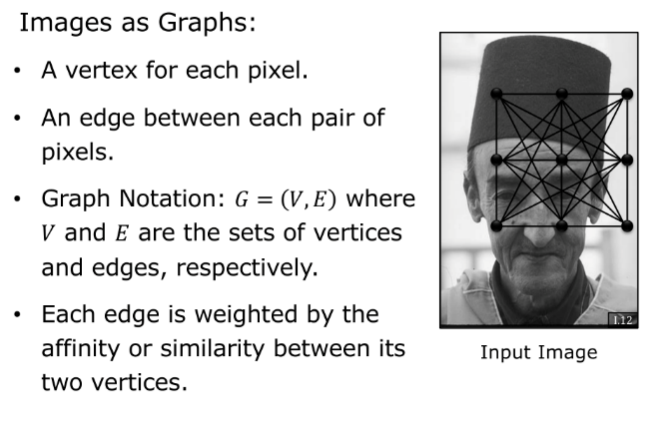
Pixel Affinity Formulation
For two pixels with feature vectors $\mathbf{f}_i$ and $\mathbf{f}_j$, their affinity $w(i,j)$ is computed via a Gaussian kernel:
$$w(i,j) = A(\mathbf{f}_i, \mathbf{f}_j) = e^{-\frac{1}{2\sigma^2} |\mathbf{f}_i - \mathbf{f}_j|^2}$$
- High similarity ($|\mathbf{f}_i - \mathbf{f}_j| \to 0$) yields large edge weight ($w(i,j) \to 1$).
- $\sigma$ controls sensitivity to feature differences.
6.2 Graph Cuts and Minimum Cut (Min-Cut)
- Cut: A partition of vertices $V$ into two disjoint subsets $V_A$ and $V_B$ ($V_A \cup V_B = V, V_A \cap V_B = \emptyset$).
- Cut-Set: The set of edges crossing the partition boundary.
- Cost of Cut: The sum of weights of all cut-set edges:
$$\text{cut}(V_A, V_B) = \sum_{u \in V_A, , v \in V_B} w(u,v)$$
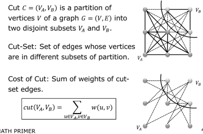
The Bias Flaw of Min-Cut
Minimizing $\text{cut}(V_A, V_B)$ directly (Min-Cut) has a severe structural flaw: it is heavily biased toward carving out tiny, isolated pixels or corner fragments.
- Reason: The cost of cutting 100 weak edges across a large object boundary is much greater than cutting 1 strong edge connecting a single isolated corner pixel. Min-Cut trivializes the objective by shaving off individual pixels.
6.3 Normalized Cut (NCut)
Jianbo Shi and Jitendra Malik (2000) resolved this bias by normalizing the cut cost against the total association of each sub-graph with the entire graph.
1. Subgraph Association
The total connection weight of subgraph $V_A$ with the full graph $V$ is defined as Association:
$$\text{assoc}(V_A, V) = \sum_{u \in V_A, , v \in V} w(u,v)$$
2. NCut Formulation
The Normalized Cut cost is defined as:
$$\text{NCut}(V_A, V_B) = \frac{\text{cut}(V_A, V_B)}{\text{assoc}(V_A, V)} + \frac{\text{cut}(V_A, V_B)}{\text{assoc}(V_B, V)}$$
- If one subgraph is tiny (e.g., $V_A$ has only 1 pixel), its $\text{assoc}(V_A, V)$ is minuscule, causing the quotient to explode and heavily penalizing unbalanced cuts.
- The objective reaches its minimum only when both partitions are substantial and balanced.
3. Spectral Solution (Shi & Malik, 2000)
- NP-Completeness: Minimizing discrete $\text{NCut}$ is NP-Complete.
- Spectral Relaxation: Shi & Malik relaxed the discrete indicator vector into continuous domain, transforming it into a generalized eigenvalue problem: $$(D - W)\mathbf{y} = \lambda D \mathbf{y}$$ where $W$ is the affinity matrix and $D$ is the diagonal degree matrix ($D_{ii} = \sum_j W_{ij}$). The eigenvector corresponding to the second smallest eigenvalue (the Fiedler vector) provides the optimal continuous partition.
7. Summary Comparison Matrix
| Algorithm Class | Core Decision / Mathematical Formula | User Parameters | Key Advantage | Primary Limitation / Failure Mode |
|---|---|---|---|---|
| k-Means | $\text{Cluster}(x_j) = \arg\min_i |\mathbf{f}_j - m_i|$ | Cluster count $k$ | Simple, fast, easily parallelizable | Requires predefined $k$, sensitive to initialization, corrupted by outliers |
| Mean-Shift | $m_i \leftarrow \text{centroid}(W(m_i))$ (Hill-Climbing) | Window radius $W$ (Bandwidth) | Discovers $k$ automatically; handles arbitrary non-convex shapes and outliers | High computational cost per pixel; highly sensitive to bandwidth $W$ |
| Min-Cut (Graph) | $\min \sum_{u \in V_A, v \in V_B} w(u,v)$ | None (pure min-cut) | Global optimization of boundary contrast | Severe bias toward peeling off small, isolated single pixels |
| Normalized-Cut (NCut) | $\min \left( \frac{\text{cut}(V_A, V_B)}{\text{assoc}(V_A, V)} + \frac{\text{cut}(V_A, V_B)}{\text{assoc}(V_B, V)} \right)$ | Relaxation threshold / Eigenvector cut | Balanced, meaningful object-level segments | NP-Complete; requires spectral continuous eigenvalue relaxation |
Appearance Representation and PCA Mathematics
- 1. Overview and Introduction
- 2. Shape vs. Appearance Representations
- 3. Learning Appearance and Preprocessing
- 4. Principal Component Analysis (PCA)
- 5. Mathematical Derivation of Principal Components
- 6. Summary and Next Steps
This lecture note covers the paradigm shift in computer vision from geometric modeling to signal-based appearance modeling, visual representations in high-dimensional pixel space, data acquisition and brightness normalization pipelines, and the linear algebraic heart of dimensionality reduction: Principal Component Analysis (PCA) with full step-by-step Lagrange multiplier derivations, based on the curriculum from the Columbia University CAVE Lab (Prof. Shree K. Nayar).
1. Overview and Introduction
In computer vision, traditional approaches to object recognition and pose estimation focused on reconstructing explicit three-dimensional (3D) geometric models of objects and matching them against 3D sensor data. However, the hardware complexity, computational cost, and sensitivity to noise of 3D acquisition led researchers to explore directly using 2D visual intensity patterns (signals) captured by cameras.
Appearance Matching is a powerful computer vision paradigm that models objects not by explicit 3D geometry, but by the holistic visual patterns produced across varying viewpoints (poses) and lighting conditions (illumination).
flowchart LR
Scene["Real-World Object\n(Physical 3D Entity)"] --> Light["Illumination Direction (ω₂)"]
Scene --> Pose["Pose / Rotation Angle (ω₁)"]
Light & Pose --> Cam["Camera Projection"]
Cam --> Img["2D Pixel Intensity Pattern\n(Appearance Signal I)"]
Img --> PCA["PCA Dimensionality Reduction\n(Low-Dimensional Subspace)"]
PCA --> Match["Real-Time Recognition &\nPose / Light Estimation"]
style Scene fill:#1a1a2e,stroke:#e94560,color:#fff
style Light fill:#16213e,stroke:#4cc9f0,color:#fff
style Pose fill:#16213e,stroke:#4cc9f0,color:#fff
style Cam fill:#0f3460,stroke:#e94560,color:#fff
style Img fill:#1a1a2e,stroke:#4cc9f0,color:#fff
style PCA fill:#53354a,stroke:#e94560,color:#fff
style Match fill:#16213e,stroke:#4cc9f0,color:#fff
The primary objective is to compress massive visual data from a high-dimensional pixel space (e.g., $200 \times 200 = 40,000$ dimensions) into a much lower-dimensional mathematical subspace while retaining maximum discriminative variance.
2. Shape vs. Appearance Representations
2.1 Explicit 3D Geometry Representations
In computer graphics, CAD/CAM, and manufacturing, objects are represented using explicit 3D mathematical descriptions:
- Voxel Representation: The 3D volumetric generalization of 2D pixels (volume element). Space is discretized into 3D grids storing occupancy binary or density values.
- Surface Primitives: Defines boundaries of opaque objects using planar polygon meshes, spheres, or parametric patches.
- Superquadrics: Analytical geometric primitives capable of expressing a continuous spectrum from sharp corners to smooth cylindrical and spherical bodies with a single compact formula:
$$|x|^r + |y|^s + |z|^t = 1$$
Here, $r, s, t$ are real parameters. Varying these exponents morphs the shape between cubes, cylinders, cones, and ellipsoids.
- Constructive Solid Geometry (CSG): Constructs complex industrial parts by combining basic primitives (spheres, cubes, cylinders) via Boolean set operations: Union, Difference, and Intersection.
2.2 Challenges of 3D Shape Modeling in Computer Vision
While geometric models are ideal for manufacturing and rendering, they present significant hurdles for vision-based recognition:
- Explicit Model Acquisition Overhead: Requires laborious manual CAD modeling or high-precision structured light/laser range scanning for every single object in the database.
- Online 3D Depth Sensing Requirement: At runtime, the scene must be scanned with depth sensors (e.g., LiDAR, RGB-D) to generate noisy 3D point clouds.
- Alignment and Search Complexity: Matching 3D point clouds or CAD meshes (e.g., via ICP) is computationally expensive, prone to local minima, and fragile against occlusion.
2.3 Appearance-Based Approach
The appearance-based approach bypasses explicit 3D geometry by directly modeling the 2D optical intensity map captured by the sensor. An observed image is a combined function of two parameter categories:
$$\text{Visual Appearance} = \mathcal{F}(\text{Intrinsic Parameters}, \text{Extrinsic Parameters})$$
- Intrinsic Parameters: Inherent, observer-independent physical properties of the object that remain invariant over time. These include 3D shape and surface reflectance (BRDF - Bidirectional Reflectance Distribution Function).
- Extrinsic Parameters: Observer-dependent variables that change continuously in real time, including 3D pose relative to the camera (Pose $\boldsymbol{\omega}_1$) and illumination direction/strength (Illumination $\boldsymbol{\omega}_2$).
Core Insight: Rather than explicitly recovering 3D geometry and BRDF, we directly learn the low-dimensional manifold formed by all 2D image variations produced across extrinsic parameters ($\boldsymbol{\omega} = [\omega_1, \omega_2]^T$).
3. Learning Appearance and Preprocessing
The machine learning methodology for appearance modeling mirrors human visual cognition. When humans inspect an unfamiliar object, they rotate it in their hands under various light sources to form an internal visual representation across orientations.
3.1 Acquiring the Object Image Set
To automate and standardize this process, a controlled laboratory apparatus is used:
- Turntable (Pose Parameter $\omega_1$): The object is placed on a motorized turntable in one of its stable configurations. The table rotates $360^\circ$ to sample pose angles $\omega_1$ at discrete intervals (e.g., every $5^\circ$).
- Robotic Lighting Arm (Illumination Parameter $\omega_2$): A light source mounted on a robotic manipulator traverses a hemisphere around the object, systematically varying the illumination angle $\omega_2$.
- Stationary Camera: For each $(\omega_1, \omega_2)$ state, a high-resolution image is acquired, producing a comprehensive Object Image Set.
3.2 Preprocessing Pipeline
To ensure all captured images are directly pixel-wise comparable (metric comparability), three preprocessing stages are applied:
flowchart LR
Raw["Raw Image"] --> Seg["1. Background Segmentation\n(Masking & Zeroing)"]
Seg --> Resize["2. Canonical Resizing\n(P × Q = N Pixels)"]
Resize --> Norm["3. Vectorial Brightness Normalization\n(I_hat = I / ||I||)"]
Norm --> Feat["Canonical Feature Vector (f')\n(On Unit Sphere)"]
style Raw fill:#1a1a2e,stroke:#e94560,color:#fff
style Seg fill:#16213e,stroke:#4cc9f0,color:#fff
style Resize fill:#0f3460,stroke:#4cc9f0,color:#fff
style Norm fill:#53354a,stroke:#e94560,color:#fff
style Feat fill:#1a1a2e,stroke:#4cc9f0,color:#fff
- Segmentation: Objects are imaged against a uniform dark background, which is segmented out and set to zero intensity to eliminate background clutter.
- Canonical Resizing: The bounding box of the segmented object is computed, and the object is normalized to a fixed canonical resolution (e.g., $128 \times 128$ or $200 \times 200$ pixels).
- Vectorial Brightness Normalization: To prevent lamp fluctuations, sensor sensitivity, or exposure shifts from distorting distances, the image matrix $I$ is reshaped into a vector and divided by its $L_2$ norm:
$$\hat{\mathbf{I}} = \frac{I}{|I|} = \frac{I}{\sqrt{\sum_{x,y} I(x,y)^2}}$$
This projects every image vector onto a high-dimensional Unit Sphere, decoupling appearance representation from absolute light energy.
4. Principal Component Analysis (PCA)
4.1 High-Dimensional Pixel Space
Each preprocessed canonical image contains $P \times Q = N$ pixels. By unrolling the 2D image matrix column-wise (or row-wise), we obtain an $N \times 1$ Feature Vector ($\mathbf{f}’$).
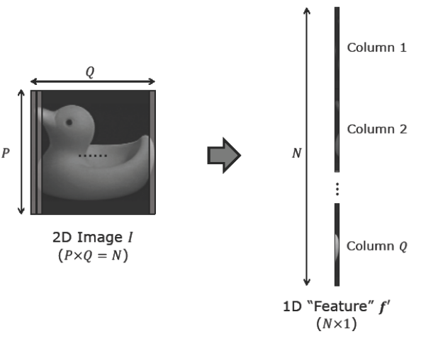
Each image is thus represented as a single point in an $N$-dimensional Euclidean space:
- Each coordinate axis corresponds to the intensity of a specific pixel location.
- The standard basis vectors ${\mathbf{i}_1, \mathbf{i}_2, \dots, \mathbf{i}_N}$ form an orthonormal basis:
$$\mathbf{i}_1 = \begin{bmatrix} 1 \ 0 \ \vdots \ 0 \end{bmatrix}, \quad \mathbf{i}_2 = \begin{bmatrix} 0 \ 1 \ \vdots \ 0 \end{bmatrix}, \quad \dots, \quad \mathbf{i}_N = \begin{bmatrix} 0 \ 0 \ \vdots \ 1 \end{bmatrix}$$
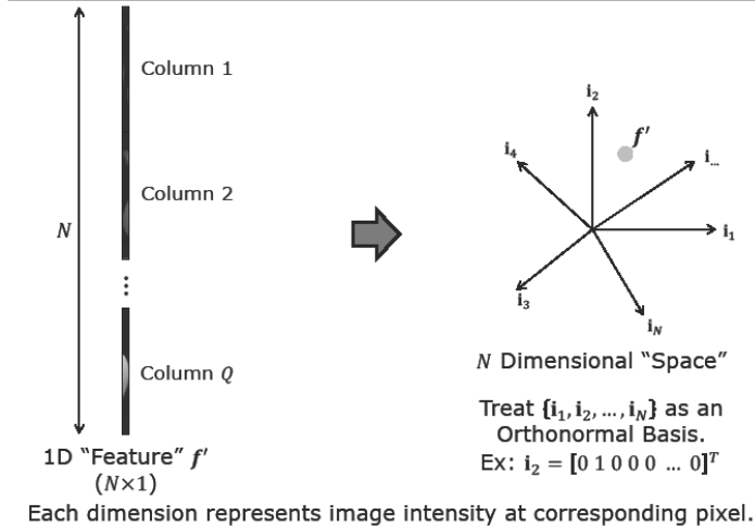
4.2 Equivalence Between Image SSD and $N$-D Euclidean Distance
The classic Sum of Squared Differences (SSD) metric between two images $I_1$ and $I_2$ is mathematically identical to the squared $L_2$ Euclidean distance between their corresponding feature vectors in $N$-dimensional space:
$$\text{SSD} = \sum_{p=1}^P \sum_{q=1}^Q \left( I_1[p,q] - I_2[p,q] \right)^2 \equiv d^2 = |\mathbf{f}‘_1 - \mathbf{f}’_2|^2$$
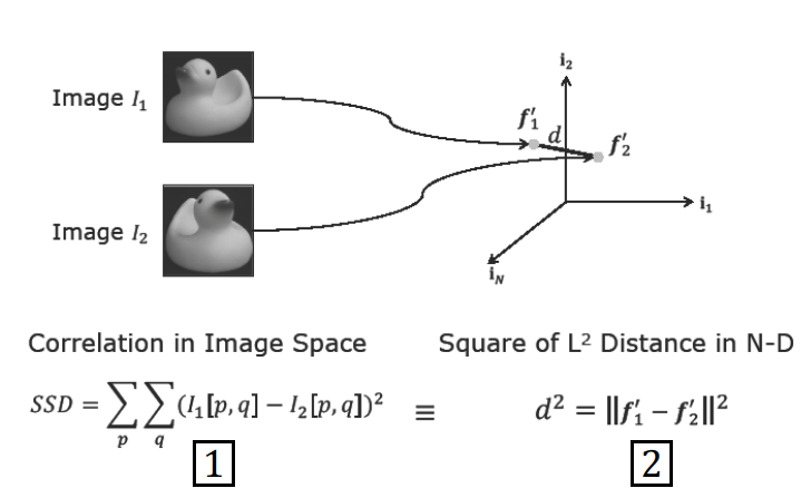
4.3 Curse of Dimensionality and Visual Redundancy
For a $200 \times 200$ image, $N = 40,000$. Performing exhaustive template matching across thousands of objects in a 40,000-dimensional space is computationally intractable.
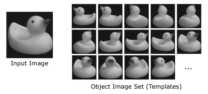
However, sequentially sampled turntable images exhibit immense visual redundancy (correlation) between neighboring frames:
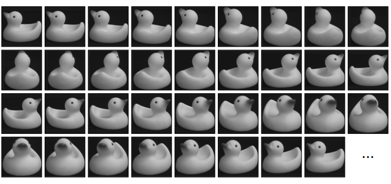
Because neighboring pixel values change smoothly, the $M$ sample points do not span the entire 40,000-dimensional space, but are tightly clustered within a low-dimensional ($K \ll N$, e.g., $K = 8 \sim 20$) Linear Subspace (Eigenspace).
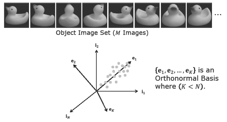
4.4 Mean Subtraction and Centering
The first step of PCA is computing the Average Image Vector ($\mathbf{c}$) across the $M$ sample images:
$$\mathbf{c} = \frac{1}{M} \sum_{m=1}^M \mathbf{f}’_m$$
Each image is then zero-centered by subtracting this mean vector:
$$\mathbf{f}_m = \mathbf{f}’_m - \mathbf{c}$$
This shifts the dataset centroid to the origin $(0,0,\dots,0)$, ensuring $E[\mathbf{f}] = \mathbf{0}$.
5. Mathematical Derivation of Principal Components
The 1st Principal Component $\mathbf{e}_1$ is the unit direction vector along which the centered data exhibits maximum variance. This corresponds to the best-fitting line in the least squares sense.
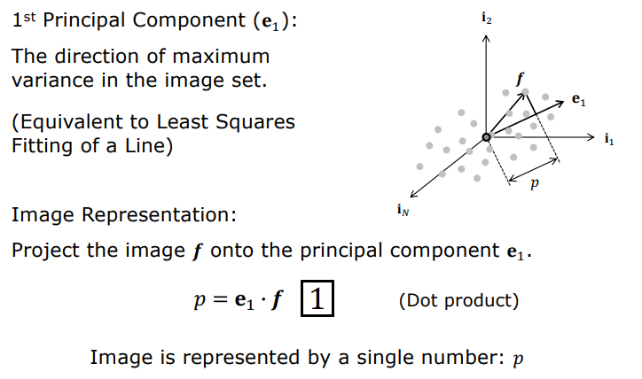
5.1 Step-by-Step Proof via Lagrange Multipliers
Step 1: Scalar Projection
The scalar coordinate $p$ of a centered image vector $\mathbf{f}$ along unit direction $\mathbf{e}$ is given by the inner product:
$$p = \mathbf{e} \cdot \mathbf{f} = \mathbf{e}^T \mathbf{f}$$
Step 2: Expected Value of Projections
Since the data is zero-centered ($E[\mathbf{f}] = \mathbf{0}$):
$$E[p] = E[\mathbf{e}^T \mathbf{f}] = \mathbf{e}^T E[\mathbf{f}] = \mathbf{e}^T \mathbf{0} = 0$$
Step 3: Variance of Projections
From the definition of variance:
$$\text{Var}(p) = E\left[ (p - E[p])^2 \right] = E\left[ p^2 \right] = E\left[ (\mathbf{e}^T \mathbf{f})^2 \right]$$
Expanding the squared scalar using transpose properties:
$$(\mathbf{e}^T \mathbf{f})^2 = (\mathbf{e}^T \mathbf{f})(\mathbf{e}^T \mathbf{f})^T = (\mathbf{e}^T \mathbf{f})(\mathbf{f}^T \mathbf{e}) = \mathbf{e}^T (\mathbf{f} \mathbf{f}^T) \mathbf{e}$$
Pulling the constant vector $\mathbf{e}$ outside the expectation:
$$\text{Var}(p) = \mathbf{e}^T E\left[ \mathbf{f} \mathbf{f}^T \right] \mathbf{e}$$
Here, $E[\mathbf{f} \mathbf{f}^T]$ is the $N \times N$ Covariance Matrix ($R$):
$$R = E[\mathbf{f} \mathbf{f}^T] = \frac{1}{M} \sum_{m=1}^M \mathbf{f}_m \mathbf{f}_m^T$$
Thus, the variance simplifies to a quadratic form:
$$\text{Var}(p) = \mathbf{e}^T R \mathbf{e}$$
Step 4: Unit Vector Constraint and Lagrange Multiplier
To prevent $|\mathbf{e}| \to \infty$, we enforce the unit norm constraint:
$$|\mathbf{e}|^2 = 1 \implies \mathbf{e}^T \mathbf{e} = 1 \implies \mathbf{e}^T \mathbf{e} - 1 = 0$$
Formulating the Lagrangian objective function $\mathcal{L}(\mathbf{e}, \lambda)$:
$$\mathcal{L}(\mathbf{e}, \lambda) = \mathbf{e}^T R \mathbf{e} - \lambda (\mathbf{e}^T \mathbf{e} - 1)$$
Step 5: Partial Derivative and Eigenvalue Equation
Setting the gradient with respect to $\mathbf{e}$ to zero:
$$\frac{\partial \mathcal{L}}{\partial \mathbf{e}} = 2 R \mathbf{e} - 2 \lambda \mathbf{e} = \mathbf{0}$$
Dividing by 2 yields the canonical Eigenvalue/Eigenvector Equation:
$$R \mathbf{e} = \lambda \mathbf{e}$$
Step 6: Equivalence of Variance and Eigenvalue
Substituting $R \mathbf{e} = \lambda \mathbf{e}$ back into the variance formula:
$$\text{Var}(p) = \mathbf{e}^T (R \mathbf{e}) = \mathbf{e}^T (\lambda \mathbf{e}) = \lambda (\mathbf{e}^T \mathbf{e})$$
Since $\mathbf{e}^T \mathbf{e} = 1$:
$$\text{Var}(p) = \lambda$$
Fundamental Theorem: The variance of projected data along direction $\mathbf{e}$ is exactly equal to the eigenvalue $\lambda$. Maximizing variance corresponds directly to finding the largest eigenvalue ($\lambda_1$) and its associated eigenvector ($\mathbf{e}_1$) of the covariance matrix $R$.
5.2 Multi-Dimensional Eigenspace Construction
The second principal component $\mathbf{e}_2$ is the eigenvector corresponding to the second largest eigenvalue $\lambda_2$, constrained to be orthogonal to $\mathbf{e}_1$ ($\mathbf{e}_1 \perp \mathbf{e}_2$).
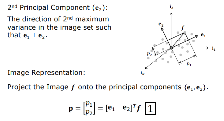
Sorting the eigenvectors in descending order of eigenvalues ($\lambda_1 \ge \lambda_2 \ge \dots \ge \lambda_K$), we construct the $N \times K$ Eigenspace Matrix ($E$):
$$E = \begin{bmatrix} \mathbf{e}_1 & \mathbf{e}_2 & \dots & \mathbf{e}K \end{bmatrix}{N \times K}$$
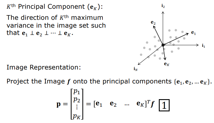
5.3 Forward and Back Projection
- Forward Projection (Encoding / Compression): Any centered image vector $\mathbf{f}$ is compressed into a $K$-dimensional coordinate vector $\mathbf{p}$:
$$\mathbf{p} = \begin{bmatrix} p_1 \ p_2 \ \vdots \ p_K \end{bmatrix} = \begin{bmatrix} \mathbf{e}_1 & \mathbf{e}_2 & \dots & \mathbf{e}_K \end{bmatrix}^T \mathbf{f} = E^T \mathbf{f}$$
- Back Projection (Reconstruction): Reconstructing the original $N$-dimensional image from coordinates $\mathbf{p}$:
$$\mathbf{f} \approx \sum_{k=1}^K p_k \mathbf{e}_k = E \mathbf{p}$$
Adding back the mean image reconstructs the uncentered image:
$$\mathbf{f}’ \approx \mathbf{c} + \sum_{k=1}^K p_k \mathbf{e}_k$$
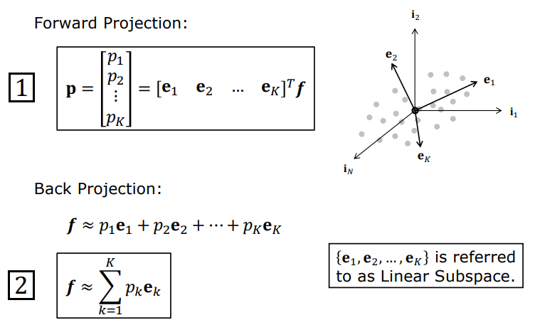
6. Summary and Next Steps
| Concept | Mathematical Formulation | Role & Meaning |
|---|---|---|
| Vector Normalization | $\hat{\mathbf{I}} = I / |I|$ | Normalizes brightness and exposure onto the unit sphere. |
| Average Image | $\mathbf{c} = \frac{1}{M}\sum \mathbf{f}’_m$ | Centroid of the dataset in $N$-D space. |
| Covariance Matrix | $R = \frac{1}{M}\sum \mathbf{f}_m \mathbf{f}_m^T$ | $N \times N$ matrix capturing inter-pixel variances. |
| Eigenvalue Problem | $R \mathbf{e} = \lambda \mathbf{e}$ | Computes principal variance directions ($\mathbf{e}$) and amounts ($\lambda$). |
| Forward Projection | $\mathbf{p} = E^T \mathbf{f}$ | Compresses an $N$-D pixel vector into a $K$-D coordinate vector. |
| Back Projection | $\mathbf{f} \approx E \mathbf{p}$ | Reconstructs original image with minimal information loss. |
Next Lecture: Computing the eigendecomposition of a massive $40,000 \times 40,000$ matrix $R$ is computationally intractable directly. In the next lecture, we will explore Singular Value Decomposition (SVD) to solve this in seconds, fit continuous Parametric Appearance Manifolds using cubic splines, and implement real-time Appearance Matching algorithms.
SVD Optimization, Parametric Manifolds, and Appearance Matching
- 1. Linear Algebraic Proof of the PCA and SVD Equivalence
- 2. Parametric Appearance Representation
- 3. Appearance Matching (Online Recognition Pipeline)
- 4. Key Real-World Applications
- 5. Summary and Comparison
This lecture note covers the theoretical and linear algebraic bridge of Singular Value Decomposition (SVD) to overcome computational bottlenecks in large-scale PCA, the continuous geometric interpolation of Parametric Appearance Manifolds on eigenspaces, real-time Appearance Matching algorithms, and foundational computer vision applications such as Eigenfaces, Visual Servoing, and automated quality inspection, based on the curriculum from the Columbia University CAVE Lab (Prof. Shree K. Nayar).
1. Linear Algebraic Proof of the PCA and SVD Equivalence
In the previous lecture, we established that extracting principal components from $N$-pixel images requires solving an eigenvalue problem ($R \mathbf{e} = \lambda \mathbf{e}$) on an $N \times N$ covariance matrix $R$. However, in practical computer vision applications, this direct approach encounters a severe computational barrier:
- Dimensionality Explosion: For typical $200 \times 200 = 40,000$ pixel images, the covariance matrix $R$ is a gigantic $40,000 \times 40,000$ matrix ($\approx 1.6 \text{ billion floating-point numbers}$).
- Computational Infeasibility: Allocating $R$ in memory requires $\sim 6.4 \text{ GB}$ of RAM, and standard $\mathcal{O}(N^3)$ eigenvalue solvers freeze processors for extended periods.
To eliminate this bottleneck, we never construct the $N \times N$ covariance matrix explicitly. Instead, we apply Singular Value Decomposition (SVD) directly to the raw centered data matrix.
flowchart TD
Raw["M Centered Images (N x 1)"] --> Mat["Data Matrix F (N x M)"]
Mat -->|"Traditional Path: Slow"| Cov["Covariance Matrix R = F F^T (N x N)<br/>40,000 x 40,000 Memory Load"]
Cov -->|"O(N^3) Eigendecomposition"| Eig["Eigenvectors e_i and Eigenvalues lambda_i"]
Mat -->|"Modern SVD Bridge: Fast"| SVD["Direct SVD Factorization<br/>F = U Sigma V^T (Milliseconds)"]
SVD --> EigSVD["Columns of U = Eigenvectors e_i<br/>Squared Singular Values = Eigenvalues lambda_i"]
style Raw fill:#1a1a2e,stroke:#e94560,color:#fff
style Mat fill:#16213e,stroke:#4cc9f0,color:#fff
style Cov fill:#53354a,stroke:#e94560,color:#fff
style Eig fill:#53354a,stroke:#e94560,color:#fff
style SVD fill:#0f3460,stroke:#4cc9f0,color:#fff
style EigSVD fill:#0f3460,stroke:#4cc9f0,color:#fff
1.1 Mathematical Proof Bridge
Let us construct an $N \times M$ Data Matrix $F$ by stacking our $M$ mean-subtracted image vectors column-wise ($M \ll N$, e.g., $M = 360$ sample images, $N = 40,000$ pixels):
$$F = \begin{bmatrix} \mathbf{f}_1 & \mathbf{f}_2 & \dots & \mathbf{f}_M \end{bmatrix}$$
The sample covariance matrix $R$ is expressed as:
$$R = F F^T$$
By the fundamental SVD theorem, any rectangular matrix $F$ can be uniquely factorized into the product of three matrices:
$$F = U \Sigma V^T$$
Where:
- $U$ ($N \times N$) and $V$ ($M \times M$) are orthonormal matrices ($U^T U = I$ and $V^T V = I$).
- $\Sigma$ ($N \times M$) is a diagonal matrix containing non-negative, sorted singular values ($\sigma_1 \ge \sigma_2 \ge \dots \ge \sigma_M \ge 0$) along its main diagonal.
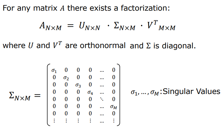
Substituting the SVD representation of $F$ into $R = F F^T$:
$$R = F F^T = (U \Sigma V^T) (U \Sigma V^T)^T$$
Applying the matrix transpose property $(A B C)^T = C^T B^T A^T$:
$$R = (U \Sigma V^T) (V \Sigma^T U^T) = U \Sigma (V^T V) \Sigma^T U^T$$
Because $V$ is orthonormal, $V^T V = I$ simplifies to the identity matrix:
$$R = U (\Sigma \Sigma^T) U^T$$
Defining the diagonal matrix $\Lambda = \Sigma \Sigma^T$ of size $N \times N$:
$$\Lambda = \Sigma \Sigma^T = \begin{bmatrix} \sigma_1^2 & 0 & \dots & 0 \ 0 & \sigma_2^2 & \dots & 0 \ \vdots & \vdots & \ddots & \vdots \ 0 & 0 & \dots & 0 \end{bmatrix}$$
Post-multiplying both sides by $U$ (using $U^T U = I$):
$$R = U \Lambda U^T \implies R U = U \Lambda$$
Examining each column $\mathbf{u}_i$ of matrix $U$:
$$R \mathbf{u}_i = \lambda_i \mathbf{u}_i \quad \text{where} \quad \lambda_i = \sigma_i^2$$
Key Linear Algebra Equivalence:
- The columns of $U$ ($\mathbf{u}_i$) resulting from the SVD of the raw data matrix $F$ are exactly the eigenvectors ($\mathbf{e}_i$) of the covariance matrix $R$.
- The eigenvalues ($\lambda_i$) of the covariance matrix equal the squared singular values ($\sigma_i^2$) of $F$.
Because thin/truncated SVD only computes $\min(N, M) = M$ components, execution time drops from minutes to milliseconds!
2. Parametric Appearance Representation
2.1 Subspace Dimension ($K$) Selection via Energy Criterion
Due to substantial correlation (visual redundancy) across neighboring turntable views, the eigenvalues $\lambda_k$ decay rapidly. Beyond the first few components, subsequent eigenvalues drop close to zero.
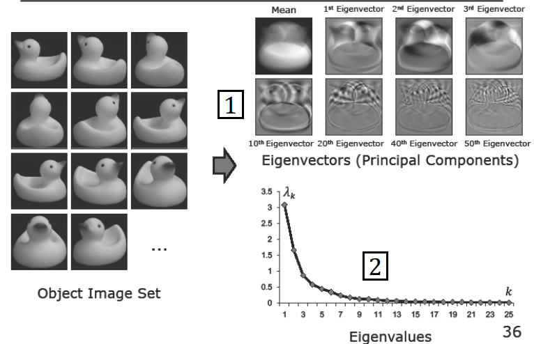
To retain $95%$ of the total data energy (variance), the optimal subspace dimension $K$ is selected via the cumulative eigenvalue ratio:
$$\text{Find smallest } K \text{ such that:} \quad \frac{\sum_{i=1}^{K} \lambda_i}{\sum_{j=1}^{N} \lambda_j} \ge 0.95$$
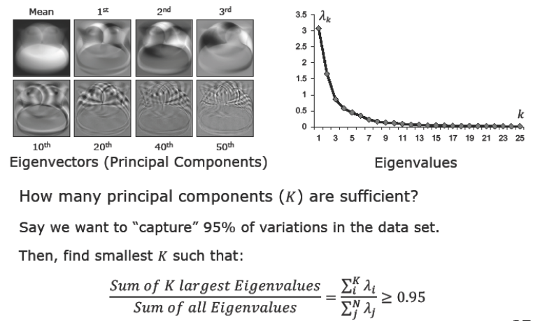
In practice, a 40,000-dimensional pixel space is compressed into a $K = 8 \sim 20$ dimensional eigenspace, achieving a $2,000 \times$ to $5,000 \times$ compression ratio with near-zero perceptual degradation.
2.2 Eigenspace Projection and Extrinsic Parameters
An object’s observed image is parameterized by intrinsic physical properties and extrinsic observation variables ($\boldsymbol{\omega}$):
$$\boldsymbol{\omega} = \begin{bmatrix} \omega_1 \ \omega_2 \ \vdots \ \omega_T \end{bmatrix} = \begin{bmatrix} \text{Pose Angle} \ \text{Illumination Direction} \ \vdots \end{bmatrix}$$
A normalized image vector $\mathbf{f}’(\boldsymbol{\omega})$ at parameter state $\boldsymbol{\omega}$ is projected into the eigenspace after mean subtraction:
$$\mathbf{p}(\boldsymbol{\omega}) = \begin{bmatrix} \mathbf{e}_1 & \mathbf{e}_2 & \dots & \mathbf{e}_K \end{bmatrix}^T (\mathbf{f}’(\boldsymbol{\omega}) - \mathbf{c})$$
This transforms an entire 40,000-pixel image into a single coordinate point $\mathbf{p}(\boldsymbol{\omega})$ in $K$-dimensional space.
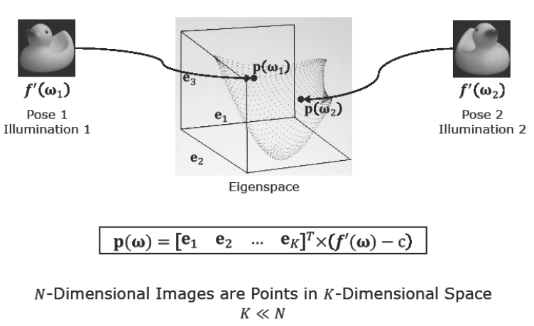
2.3 Constructing the Continuous Appearance Manifold
Because sample images are recorded at discrete intervals (e.g., every $5^\circ$ or $10^\circ$), the projected points $\mathbf{p}(\boldsymbol{\omega}_m)$ form a discrete trajectory.
- Cubic Spline Interpolation: A low-degree continuous surface interpolation (cubic splines) is fitted across the discrete projection points.
- Closed Manifold Geometry: Because rotating $360^\circ$ returns to the starting orientation, the resulting surface curves back onto itself, creating a smooth, continuous, and Closed Appearance Manifold.
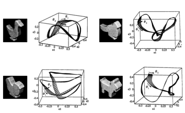
3. Appearance Matching (Online Recognition Pipeline)
Once continuous manifolds $\mathbf{p}^{(q)}(\boldsymbol{\omega})$ are learned for all database objects $q = 1 \dots Q$, runtime recognition proceeds via the following pipeline:
flowchart TD
Input["Input Test Image (I)"] --> Pre["1. Preprocessing:<br/>Background Segmentation and Canonical Resizing"]
Pre --> Norm["2. Vector Normalization:<br/>I_hat = I / norm(I)"]
Norm --> Sub["3. Mean Subtraction:<br/>f = f_hat - c^(q)"]
Sub --> Proj["4. Eigenspace Projection:<br/>p^(q) = (E^(q))^T f"]
Proj --> Dist["5. Manifold Distance Minimization:<br/>d^(q) = min_omega norm(p^(q) - p^(q)(omega))"]
Dist --> Loop{"Evaluated for all<br/>q = 1...Q Objects?"}
Loop -->|No| Proj
Loop -->|Yes| Best["6. Identify Nearest Object:<br/>r = argmin_q d^(q)"]
Best --> Check{"d^(r) <= Threshold T?"}
Check -->|Yes| Match["Identity Confirmed: Object r<br/>3D Pose: omega_1 | Illumination: omega_2"]
Check -->|No| Unknown["Unknown / Unregistered Object"]
style Input fill:#1a1a2e,stroke:#e94560,color:#fff
style Pre fill:#16213e,stroke:#4cc9f0,color:#fff
style Norm fill:#0f3460,stroke:#4cc9f0,color:#fff
style Sub fill:#0f3460,stroke:#4cc9f0,color:#fff
style Proj fill:#53354a,stroke:#e94560,color:#fff
style Dist fill:#16213e,stroke:#4cc9f0,color:#fff
style Loop fill:#1a1a2e,stroke:#4cc9f0,color:#fff
style Best fill:#0f3460,stroke:#4cc9f0,color:#fff
style Check fill:#53354a,stroke:#e94560,color:#fff
style Match fill:#1a1a2e,stroke:#4cc9f0,color:#fff
style Unknown fill:#333,stroke:#888,color:#fff
3.1 Step-by-Step Recognition & Pose Estimation
- Preprocessing: The test image $I$ is segmented, resized to the canonical frame, and normalized: $\mathbf{f}’ = I / |I|$.
- Subspace Projection: For object $q$, the mean image $\mathbf{c}^{(q)}$ is subtracted and projected into its eigenspace:
$$\mathbf{p}^{(q)} = (E^{(q)})^T (\mathbf{f}’ - \mathbf{c}^{(q)})$$
- Distance Minimization: The minimum Euclidean distance $d^{(q)}$ between $\mathbf{p}^{(q)}$ and the continuous manifold $\mathbf{p}^{(q)}(\boldsymbol{\omega})$ is computed:
$$d^{(q)} = \min_{\boldsymbol{\omega}} |\mathbf{p}^{(q)} - \mathbf{p}^{(q)}(\boldsymbol{\omega})|$$
- Classification & Pose Recovery: The object class $r$ with the smallest minimum distance is selected:
$$r = \arg\min_q d^{(q)}$$
If $d^{(r)} \le T$, identity is classified as $r$. The optimal continuous parameter $\boldsymbol{\omega}^* = [\omega_1^, \omega_2^]^T$ simultaneously estimates 3D pose and illumination direction with sub-degree precision.
3.2 Proof of Equivalence Between Eigenspace Distance and SSD
The Euclidean distance in eigenspace is equivalent to the Sum of Squared Differences (SSD) in full pixel space:
$$d^2 = |\mathbf{p}_1 - \mathbf{p}2|^2 = \left| \sum{k=1}^{K} p_k^{(1)} \mathbf{e}k - \sum{k=1}^{K} p_k^{(2)} \mathbf{e}_k \right|^2 \approx |\mathbf{f}_1’ - \mathbf{f}_2’|^2 = \text{SSD}$$
4. Key Real-World Applications
4.1 Face Recognition: Eigenfaces (Turk & Pentland, 1991)
The Eigenfaces algorithm by Matthew Turk and Alex Pentland pioneered appearance-based recognition:
- Eigenvectors computed across human face datasets resemble ghostly faces (Eigenfaces).
- Any face image is represented as a compact linear combination (weighted sum) of these eigenfaces:
$$\text{Face Image} \approx \mathbf{c} + w_1 \mathbf{e}_1 + w_2 \mathbf{e}_2 + \dots + w_K \mathbf{e}_K$$
- Classification is achieved by matching weight vectors $[w_1, \dots, w_K]$ against the database.
4.2 Visual Servoing and Robot Positioning
In automated manufacturing (e.g., peg-in-hole insertion), a camera mounted on the robot’s end-effector observes the target workpiece:
- Without recovering 3D coordinates, displacement in eigenspace coordinates ($\Delta \mathbf{p}$) directly guides robot joint motor commands ($\text{Appearance} = \mathcal{F}{\text{Robot Coordinates}}$).
4.3 Automated Temporal Inspection
For automated quality control of printed circuit boards (PCBs) and assemblies:
- Scanning a golden (defect-free) unit generates a smooth reference trajectory curve in eigenspace.
- When new production boards are scanned, missing chips or soldering anomalies produce immediate deviations from this reference curve, instantly flagging defects.
5. Summary and Comparison
| Dimension | Classical 3D Geometric Vision | Appearance-Based (PCA + SVD + Manifold) |
|---|---|---|
| Model Representation | CAD, Polygon Mesh, Voxel, CSG | Low-dimensional Eigenspace ($K \approx 15$) & Continuous Manifold |
| Sensor Requirement | Laser Scanners / Structured Light / RGB-D | Standard 2D Camera |
| Computational Burden | Heavy 3D point cloud registration (ICP) | Millisecond $K$-dimensional Euclidean distance minimization |
| Pose & Light Recovery | Multiple complex photometric passes | Simultaneous extraction via manifold coordinate $\boldsymbol{\omega}^*$ |
| Algorithmic Efficiency | $\mathcal{O}(N^3)$ Covariance Eigendecomposition | $\mathcal{O}(M^2 N)$ Fast Truncated SVD |
Foundations of Neural Networks: Perceptron and Activation Functions
- 1. Overview and Biological Inspiration
- 2. Perceptron (Single-Layer Receiver)
- 3. Perceptron Networks and Universality
- 4. Activation Functions
- 5. Technical Comparison Matrix
This lecture note covers the initial foundation of Neural Networks in computer vision and artificial intelligence—from biological inspirations to Frank Rosenblatt’s Perceptron model, the geometry of linear decision boundaries, universality proofs via NAND gates, and the mathematical necessity of non-linear activation functions.
1. Overview and Biological Inspiration
1.1 Limits of Classical Vision and Complex Visual Mappings
In computer vision, many tasks such as edge detection, camera calibration, stereo reconstruction, or photometric stereo can be resolved using deterministic algorithms derived directly from optical and physical first principles. However, tasks that human visual perception solves effortlessly pose immense challenges for hand-crafted deterministic rules:
- Handwritten Digit Recognition (MNIST): Variations across individuals writing the same digit (e.g., “5” or “6”) exhibit immense structural diversity in stroke width, slant, ink thickness, and aspect ratio. No static geometric template or fixed linear filter set can reliably generalize across these variations.
- General Object Categorization (e.g., Chairs & Human Faces): All chairs serve the same functional purpose, yet office chairs, dining chairs, and rocking chairs possess completely distinct 3D geometries and 2D pixel projections. Similarly, human faces vary across age, gender, ethnicity, pose, and illumination, making rule-based deterministic parsing intractable.
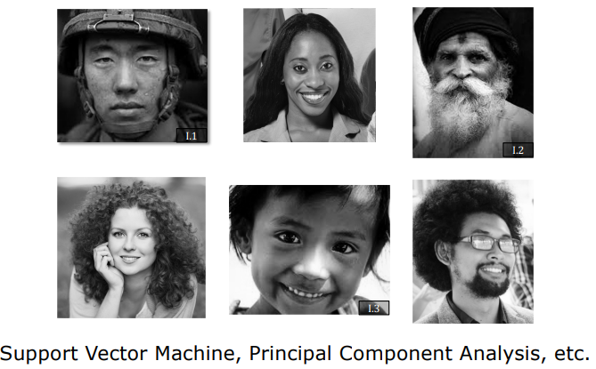
flowchart LR
Deterministic["Deterministic Models\n(Physical / Optical Laws)"] -->|"Low Variation / Closed Physics"| Classical["Edge Detection, Calibration, Stereo"]
Learned["Learning Systems\n(Biologically Inspired ANN)"] -->|"High Variation / Complex Manifolds"| Neural["Face Recognition, MNIST, Object Parsing"]
style Deterministic fill:#1a1a2e,stroke:#e94560,color:#fff
style Classical fill:#16213e,stroke:#4cc9f0,color:#fff
style Learned fill:#0f3460,stroke:#e94560,color:#fff
style Neural fill:#53354a,stroke:#e94560,color:#fff
1.2 Biological Neuron Architecture and the Brain
The human brain processes these complex non-linear visual mappings in fractions of a second. This remarkable capability emerges from a massively parallel interconnected network of billions of biological neurons, each performing simple electrochemical integrations:
- Human Brain: Weighs approximately $1.5\text{ kg}$ ($3.3\text{ lbs}$) with a volume of around $1260\text{ cm}^3$.
- Computational Scale: Contains roughly 100 Billion ($10^{11}$) neurons and 100 Trillion ($10^{14}$) synaptic interconnections.
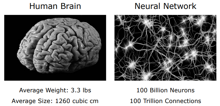
The principal anatomical building blocks of a biological neuron include:
- Dendrites & Dendritic Branches: Receptive branching fibers that collect electrochemical incoming signals from upstream neurons.
- Cell Body / Nucleus (Soma): Aggregates incoming inputs and determines the net membrane potential.
- Axon: A single conductive transmission cable that propagates an electrical action potential (spike) when the internal threshold is exceeded.
- Synaptic Terminals (Synapses): Junction points that modulate signal transmission to target dendrites via neurotransmitters. The conductivity of each synapse defines the connection “strength” (weight).
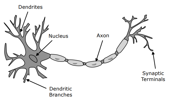
flowchart LR
subgraph Biological["Biological Neuron"]
D["Dendrites\n(Input Signals)"] --> S["Soma / Nucleus\n(Integration / Threshold)"]
S --> A["Axon & Synapses\n(Action Potential Output)"]
end
subgraph Artificial["Artificial Neuron (Perceptron)"]
X["Inputs: x₁, x₂, ..., x_d\n(Input Vector)"] --> W["Weighted Sum: Σ w_i x_i + b\n(Linear Combination z)"]
W --> F["Activation Function: f(z)\n(Output Activation a)"]
end
Biological -.->|"Analog Bridge"| Artificial
style D fill:#1a1a2e,stroke:#e94560,color:#fff
style S fill:#16213e,stroke:#4cc9f0,color:#fff
style A fill:#0f3460,stroke:#e94560,color:#fff
style X fill:#1a1a2e,stroke:#e94560,color:#fff
style W fill:#53354a,stroke:#e94560,color:#fff
style F fill:#16213e,stroke:#4cc9f0,color:#fff
2. Perceptron (Single-Layer Receiver)
The fundamental computational unit of artificial neural networks is the Perceptron. Introduced by Frank Rosenblatt (1958) at Cornell Aeronautical Laboratory, it was the first algorithmic model capable of learning binary classification boundaries from sample data.
2.1 Mathematical Formulation
A perceptron takes $d$ independent inputs $x_1, x_2, \dots, x_d$. Each input is scaled by an associated weight $w_1, w_2, \dots, w_d$, reflecting its relative significance. A constant bias term $b$ (or $-\text{threshold}$) is added to provide translational degrees of freedom to the boundary.
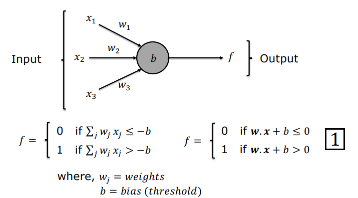
The net internal linear aggregation $z$ is formulated as an inner product:
$$z = \sum_{j=1}^d w_j x_j + b = \mathbf{w}^T \mathbf{x} + b$$
Where:
- $\mathbf{w} = [w_1, w_2, \dots, w_d]^T$ : Weight vector.
- $\mathbf{x} = [x_1, x_2, \dots, x_d]^T$ : Input vector.
- $b$ : Bias parameter.
The final output activation $a$ is produced by applying a sharp Heaviside (Step) activation function:
$$a = f(z) = \begin{cases} 1, & \text{if } z > 0 \quad (\mathbf{w}^T \mathbf{x} + b > 0) \ 0, & \text{if } z \leq 0 \quad (\mathbf{w}^T \mathbf{x} + b \leq 0) \end{cases}$$
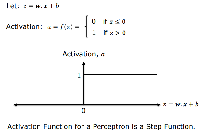
2.2 Decision Weighting Scenario (Movie Going Decision)
To demonstrate how weights prioritize competing factors in human decision-making, consider the decision: “Will you go to the movies?”
Let the decision depend on three binary conditions:
- $x_1 = 1$ (Weather is good), $x_1 = 0$ (Weather is bad)
- $x_2 = 1$ (A friend joins), $x_2 = 0$ (Alone)
- $x_3 = 1$ (Cinema is nearby), $x_3 = 0$ (Cinema is far away)
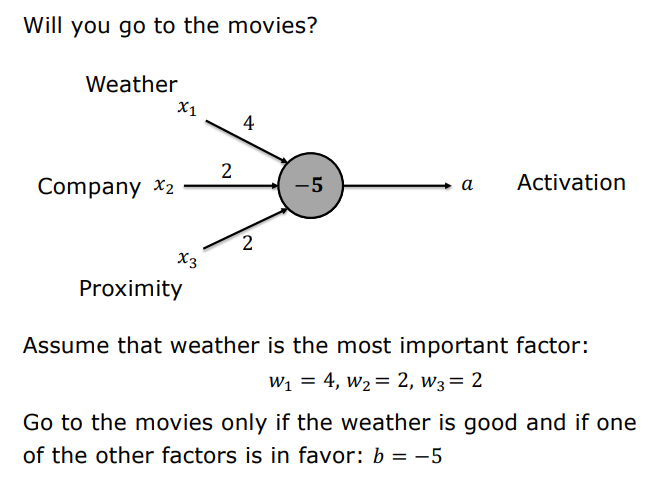
Setting weather as the dominant prerequisite implies choosing $w_1$ substantially larger than other weights:
- Parameters: $w_1 = 4$ (Weather), $w_2 = 2$ (Company), $w_3 = 2$ (Proximity), $b = -5$.
Scenario Evaluation:
- Bad Weather ($x_1 = 0$), all other conditions favorable ($x_2 = 1, x_3 = 1$): $$z = (4 \cdot 0) + (2 \cdot 1) + (2 \cdot 1) - 5 = 4 - 5 = -1$$ $z \leq 0 \implies a = 0$ (Do not go to the movies). Bad weather overrides both company and proximity.
- Good Weather ($x_1 = 1$), friend accompanies ($x_2 = 1$), cinema is far ($x_3 = 0$): $$z = (4 \cdot 1) + (2 \cdot 1) + (2 \cdot 0) - 5 = 6 - 5 = +1$$ $z > 0 \implies a = 1$ (Go to the movies).
2.3 Decision Boundary Geometry and Linear Separability
Consider a 2D input space $(x_1, x_2)$ with weights $w_1 = -2, w_2 = -2$ and bias $b = 3$.
The net aggregation line equation is: $$z = -2x_1 - 2x_2 + 3$$
Setting $z = 0$ defines the Decision Boundary:
$$-2x_1 - 2x_2 + 3 = 0 \implies x_2 = -x_1 + 1.5$$
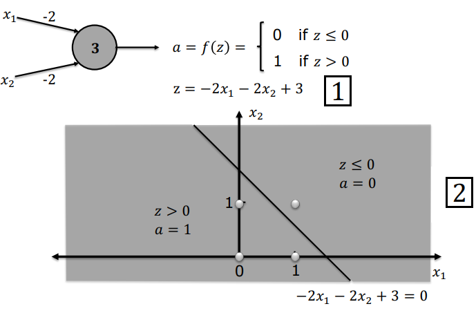
- Points lying in the lower-left half-plane yield $z > 0 \implies a = 1$.
- Points lying on or in the upper-right half-plane yield $z \leq 0 \implies a = 0$.
Linear Separability Definition: A single perceptron is fundamentally a Linear Classifier, carving a $d$-dimensional space into two halves using a $(d-1)$-dimensional flat hyperplane ($\mathbf{w}^T \mathbf{x} + b = 0$).
2.4 Minsky & Papert’s (1969) XOR Proof and the AI Winter
While single perceptrons easily separate AND, OR, and NAND functions, they cannot separate the Exclusive-OR (XOR) pattern.
| $x_1$ | $x_2$ | $x_1 \text{ XOR } x_2$ |
|---|---|---|
| 0 | 0 | 0 |
| 0 | 1 | 1 |
| 1 | 0 | 1 |
| 1 | 1 | 0 |
flowchart TD
subgraph XOR_Geometry["XOR Decision Space"]
P00["(0,0) -> Output 0"]
P11["(1,1) -> Output 0"]
P01["(0,1) -> Output 1"]
P10["(1,0) -> Output 1"]
end
Note["It is GEOMETRICALLY IMPOSSIBLE to separate (0,1) and (1,0)\nfrom (0,0) and (1,1) with a single straight line!"]
XOR_Geometry --- Note
style P00 fill:#1a1a2e,stroke:#e94560,color:#fff
style P11 fill:#1a1a2e,stroke:#e94560,color:#fff
style P01 fill:#16213e,stroke:#4cc9f0,color:#fff
style P10 fill:#16213e,stroke:#4cc9f0,color:#fff
style Note fill:#53354a,stroke:#e94560,color:#fff
Analytical Proof of Infeasibility: For a perceptron to classify XOR correctly, all four conditions must hold simultaneously:
- $(0,0) \implies b \leq 0$
- $(0,1) \implies w_2 + b > 0$
- $(1,0) \implies w_1 + b > 0$
- $(1,1) \implies w_1 + w_2 + b \leq 0$
Summing (2) and (3): $$w_1 + w_2 + 2b > 0 \implies (w_1 + w_2 + b) + b > 0$$
From (1), $b \leq 0 \implies -b \geq 0$. Thus $w_1 + w_2 + b > -b \geq 0$, giving $w_1 + w_2 + b > 0$. This directly contradicts inequality (4) ($w_1 + w_2 + b \leq 0$).
Historical Impact (AI Winter): In 1969, Marvin Minsky and Seymour Papert published “Perceptrons”, mathematically formalizing the linear limitations of single-layer models. Because general methods to train multi-layer perceptrons were unknown at the time, funding for neural network research collapsed, precipitating the first AI Winter.
3. Perceptron Networks and Universality
Connecting multiple perceptrons in parallel and hierarchical layers constructs non-linear, multi-faceted decision boundaries.
3.1 Constructing Complex and Closed Decision Regions
To isolate points inside a closed convex polygonal region in 2D space:
- First Layer (Boundary Edges): Dedicates one perceptron to each boundary line segment (e.g., 4 perceptrons for a quadrangle). Each unit outputs $1$ on the valid side of its bounding line.
- Output Layer (Logical AND / Intersection): The outputs of all 4 edge perceptrons feed into a single output perceptron with weights $\mathbf{w} = [2, 2, 2, 2]^T$ and bias $b = -7$.
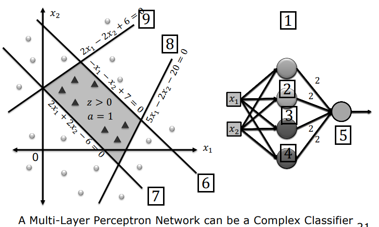
- If any single edge test fails ($0$), the maximum sum is $2 \times 3 = 6$, giving $z = 6 - 7 = -1 \leq 0 \implies a = 0$.
- Only when all 4 edge perceptrons fire simultaneously ($1$) does the sum reach $8$, yielding $z = 8 - 7 = +1 > 0 \implies a = 1$.
3.2 Proof of Perceptron as a Universal NAND Gate
Consider a 2-input perceptron with $w_1 = -2, w_2 = -2$, and $b = 3$:
| $x_1$ | $x_2$ | $z = -2x_1 - 2x_2 + 3$ | Output $a = f(z)$ | Logical Equivalent |
|---|---|---|---|---|
| 0 | 0 | $-2(0) - 2(0) + 3 = +3 > 0$ | 1 | $\text{NAND}(0,0) = 1$ |
| 0 | 1 | $-2(0) - 2(1) + 3 = +1 > 0$ | 1 | $\text{NAND}(0,1) = 1$ |
| 1 | 0 | $-2(1) - 2(0) + 3 = +1 > 0$ | 1 | $\text{NAND}(1,0) = 1$ |
| 1 | 1 | $-2(1) - 2(1) + 3 = -1 \leq 0$ | 0 | $\text{NAND}(1,1) = 0$ |
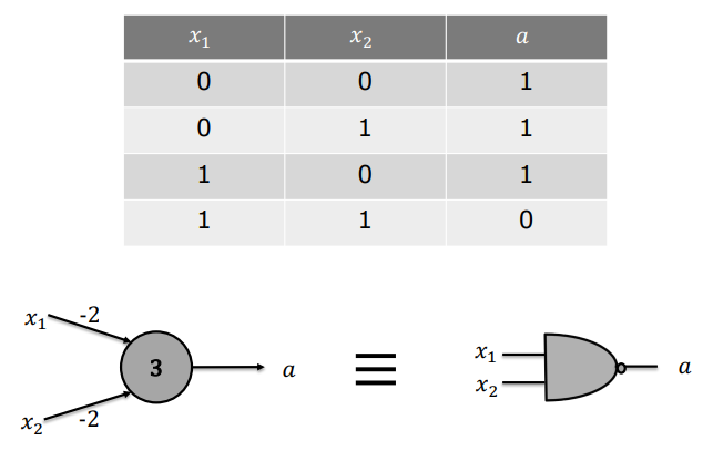
Universality of Computation Proof
In digital logic design, the NAND gate is a Universal Logic Gate. Any combinatorial digital function—including NOT, AND, OR, NOR, and XOR—can be realized purely by wiring NAND gates together.
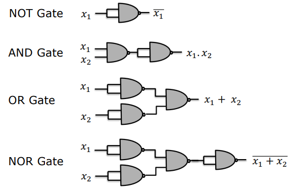
Because a single perceptron replicates a NAND gate:
- Any arbitrary digital computing architecture (ALU, registers, CPU) can be mathematically built as a network of perceptrons.
- For instance, a 1-bit binary adder producing Sum ($\text{Sum} = x_1 \oplus x_2$) and Carry ($\text{Carry} = x_1 x_2$) bits translates directly into an equivalent perceptron network.
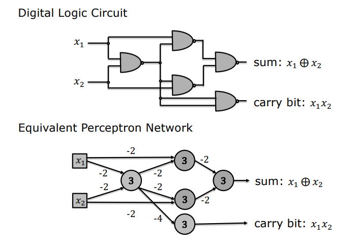
3.3 Bridge to Multilayer Network Architectures
Although perceptron networks possess theoretical computational universality, training them automatically on real-world continuous data requires structured matrix notations across layers.
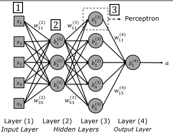
4. Activation Functions
Despite the theoretical universality of perceptron circuits, training deep networks via gradient-based optimization is impossible with discrete step functions.
4.1 Step Function Limitations and the Training Crisis
During training, we want small perturbations in parameter values ($\Delta w$ and $\Delta b$) to produce small, measurable changes in output activation ($\Delta a$):
$$\Delta a \approx \frac{\partial a}{\partial w} \Delta w$$
In step-activated perceptrons, this differential feedback is destroyed:
- Zero Gradient / Blind Region ($\Delta a = 0$): If a neuron has $z \leq 0$, perturbing a weight by $\Delta w$ keeps $z + \Delta z \leq 0$, causing zero change in output ($0 \to 0$, hence $\Delta a = 0$). Because the derivative is zero almost everywhere, gradient descent receives zero signal regarding which direction to adjust weights.
- Infinite Instability / Step Discontinuity: At the boundary $z = 0$, an infinitesimal change causes output to violently flip $0 \to 1$. Such discontinuous leaps prevent smooth, gradual parameter convergence.
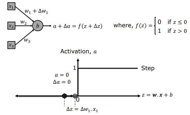
4.2 The Sigmoid Neuron
To enable continuous gradient-based learning, the discontinuous step function is replaced by the smooth, differentiable Sigmoid Activation Function ($\sigma$).
Mathematical Definition: $$\sigma(z) = \frac{1}{1 + e^{-z}}$$
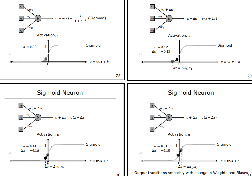
Key Properties:
- Continuous Range: $a \in (0, 1)$, enabling probabilistic interpretations of neuron confidence.
- Differentiability: A small change in weights produces a proportional, first-order Taylor approximation response: $$\Delta a \approx \sum_j \frac{\partial \sigma}{\partial w_j} \Delta w_j + \frac{\partial \sigma}{\partial b} \Delta b$$
Analytical Derivative Derivation: $$\sigma’(z) = \frac{d}{dz}\left[(1 + e^{-z})^{-1}\right] = -(1 + e^{-z})^{-2} \cdot (-e^{-z}) = \frac{e^{-z}}{(1 + e^{-z})^2}$$ $$\sigma’(z) = \frac{1}{1 + e^{-z}} \cdot \frac{e^{-z}}{1 + e^{-z}} = \sigma(z) \cdot (1 - \sigma(z))$$
This elegant identity ($\sigma’(z) = \sigma(z)(1 - \sigma(z))$) drastically speeds up backpropagation calculations by reusing forward activation values.
4.3 Why Non-Linear Activation is Mandatory
It is insufficient for an activation function to merely be continuous; it must be strictly non-linear.
Mathematical Proof (Collapse of Linear Layers): Suppose an activation function is purely linear: $f(z) = c \cdot z$. Without loss of generality, let $c = 1$ ($f(z) = z$).
In an $L$-layer network:
- Layer 1: $\mathbf{a}^{(1)} = \mathbf{W}^{(1)} \mathbf{x} + \mathbf{b}^{(1)}$
- Layer 2: $\mathbf{a}^{(2)} = \mathbf{W}^{(2)} \mathbf{a}^{(1)} + \mathbf{b}^{(2)} = \mathbf{W}^{(2)}(\mathbf{W}^{(1)} \mathbf{x} + \mathbf{b}^{(1)}) + \mathbf{b}^{(2)} = (\mathbf{W}^{(2)}\mathbf{W}^{(1)})\mathbf{x} + (\mathbf{W}^{(2)}\mathbf{b}^{(1)} + \mathbf{b}^{(2)})$
- Defining lumped parameters: $\mathbf{W}’ = \mathbf{W}^{(2)}\mathbf{W}^{(1)}$ and $\mathbf{b}’ = \mathbf{W}^{(2)}\mathbf{b}^{(1)} + \mathbf{b}^{(2)}$.
- Thus: $\mathbf{a}^{(2)} = \mathbf{W}’ \mathbf{x} + \mathbf{b}’$
Crucial Theorem: Regardless of having 2 or 1000 hidden layers, linear activations collapse the entire deep network into a single linear transformation. Such an architecture cannot solve even the XOR problem. Non-linear activations empower neural networks to warp complex geometric feature spaces into linearly separable configurations (Universal Approximation Theorem).
4.4 Comparative Analysis of Modern Activation Functions
flowchart LR
Step["Step (Heaviside)\nBinary {0,1}\nDerivative = 0"]
Sigmoid["Sigmoid σ(z)\nRange (0,1)\nVanishing Gradient"]
Tanh["Tanh(z)\nRange (-1,1)\nZero-Centered"]
ReLU["ReLU: max(0,z)\nRange [0, ∞)\nFast / No Saturation"]
LeakyReLU["Leaky ReLU\nRange (-∞, ∞)\nPrevents Dying Neurons"]
Step -->|"Smoothing"| Sigmoid
Sigmoid -->|"Zero-Centering"| Tanh
Tanh -->|"Deep Network Scale"| ReLU
ReLU -->|"Negative Slope"| LeakyReLU
style Step fill:#1a1a2e,stroke:#e94560,color:#fff
style Sigmoid fill:#16213e,stroke:#4cc9f0,color:#fff
style Tanh fill:#0f3460,stroke:#e94560,color:#fff
style ReLU fill:#53354a,stroke:#e94560,color:#fff
style LeakyReLU fill:#16213e,stroke:#4cc9f0,color:#fff
1. Hyperbolic Tangent (Tanh)
- Formula: $\tanh(z) = \frac{e^z - e^{-z}}{e^z + e^{-z}} = 2\sigma(2z) - 1$
- Output Range: $(-1, 1)$
- Derivative: $\tanh’(z) = 1 - \tanh^2(z)$
- Advantage: Zero-centered, preventing systematic zig-zag gradient dynamics during optimization.
- Limitation: Suffers from Vanishing Gradients at saturated extremes ($|z| > 3$).
2. ReLU (Rectified Linear Unit)
- Formula: $f(z) = \max(0, z)$
- Output Range: $[0, \infty)$
- Derivative: $f’(z) = \begin{cases} 1, & z > 0 \ 0, & z < 0 \end{cases}$
- Advantage: Constant non-saturating derivative ($1$) in the positive regime, mitigating vanishing gradients and computing with exceptional efficiency.
- Limitation (Dying ReLU): Neurons with inputs $z < 0$ produce zero gradients and may permanently deactivate.
3. Leaky ReLU
- Formula: $f(z) = \max(\alpha z, z) \quad (0 < \alpha \ll 1, \text{typically } \alpha = 0.01)$
- Output Range: $(-\infty, \infty)$
- Derivative: $f’(z) = \begin{cases} 1, & z > 0 \ \alpha, & z < 0 \end{cases}$
- Advantage: Maintains a small non-zero slope $\alpha$ in the negative regime, guaranteeing gradient flow and preventing permanently dead units.
5. Technical Comparison Matrix
| Activation Function | Formula | Output Range | Derivative $f’(z)$ | Key Strength | Primary Limitation |
|---|---|---|---|---|---|
| Heaviside (Step) | $f(z) = \begin{cases} 1, & z > 0 \ 0, & z \leq 0 \end{cases}$ | ${0, 1}$ | $0 \quad (\forall z \neq 0)$ | Simple digital gate logic and NAND emulation | Zero gradient everywhere; unsuitable for gradient descent optimization |
| Sigmoid | $\sigma(z) = \frac{1}{1 + e^{-z}}$ | $(0, 1)$ | $\sigma(z)(1 - \sigma(z))$ | Smooth differentiability and probabilistic output interpretation | Vanishing Gradient in saturated regions; non-zero centered |
| Tanh | $f(z) = \frac{e^z - e^{-z}}{e^z + e^{-z}}$ | $(-1, 1)$ | $1 - f(z)^2$ | Zero-centered outputs facilitating faster parameter convergence | Saturated extremes cause Vanishing Gradient |
| ReLU | $f(z) = \max(0, z)$ | $[0, \infty)$ | $\begin{cases} 1, & z > 0 \ 0, & z < 0 \end{cases}$ | Very fast evaluation; avoids gradient saturation for positive activations | Dying ReLU when units become persistently negative |
| Leaky ReLU | $f(z) = \max(\alpha z, z)$ | $(-\infty, \infty)$ | $\begin{cases} 1, & z > 0 \ \alpha, & z < 0 \end{cases}$ | Preserves continuous gradient flow on the negative axis | Hyperparameter $\alpha$ tuning requirement |
Multilayer Networks, Gradient Descent, and Backpropagation
- 1. Multi-Layer Perceptrons (MLP)
- 2. Cost Function and Gradient Descent
- 3. The Backpropagation Algorithm
- 4. Example Applications in Computer Vision
- 5. When to Use Machine Learning?
This lecture note covers the second and most foundational phase of neural networks: the Multi-Layer Perceptron (MLP) architecture, the multi-dimensional geometry of loss functions, optimization via Gradient Descent, and the analytical derivation of the Backpropagation Algorithm via the calculus chain rule.
1. Multi-Layer Perceptrons (MLP)
While single perceptrons and single-layer linear classifiers can only resolve linearly separable tasks, Multi-Layer Perceptrons (MLPs) incorporating one or more Hidden Layers can approximate arbitrary continuous non-linear mappings between high-dimensional inputs and discrete or continuous outputs.
flowchart TD
subgraph InputLayer["Input Layer (Layer 1)"]
X1["x₁ (Pixel 1)"]
X2["x₂ (Pixel 2)"]
Xdots["..."]
XN["x₇₈₄ (Pixel 784)"]
end
subgraph HiddenLayer["Hidden Layer (Layer 2)"]
H1["Neuron 1 (σ)"]
H2["Neuron 2 (σ)"]
Hdots["..."]
HM["Neuron 30 (σ)"]
end
subgraph OutputLayer["Output Layer (Layer 3/L)"]
O0["Class 0"]
O1["Class 1"]
Odots["..."]
O9["Class 9"]
end
InputLayer -->|"Weights W^(2), Biases b^(2)"| HiddenLayer
HiddenLayer -->|"Weights W^(3), Biases b^(3)"| OutputLayer
style InputLayer fill:#1a1a2e,stroke:#e94560,color:#fff
style HiddenLayer fill:#16213e,stroke:#4cc9f0,color:#fff
style OutputLayer fill:#0f3460,stroke:#e94560,color:#fff
1.1 MLP Architecture and Parametric Notation
A typical Multi-Layer Perceptron consists of three fundamental structural stages:
- Input Layer (Layer 1): Accepts raw sensory input from the external environment. The nodes perform no mathematical activation; they simply broadcast feature values (e.g., $28 \times 28 = 784$ pixel intensities in an MNIST digit).
- Hidden Layers (Layers $2 \dots L-1$): Intermediate layers containing activation units (such as Sigmoid or ReLU) that progressively extract hierarchically richer semantic representations (edges, textures, corners, parts).
- Output Layer (Layer $L$): Produces the final network prediction. In an MNIST digit recognition task, this layer contains 10 output units representing class categories from $0$ to $9$.
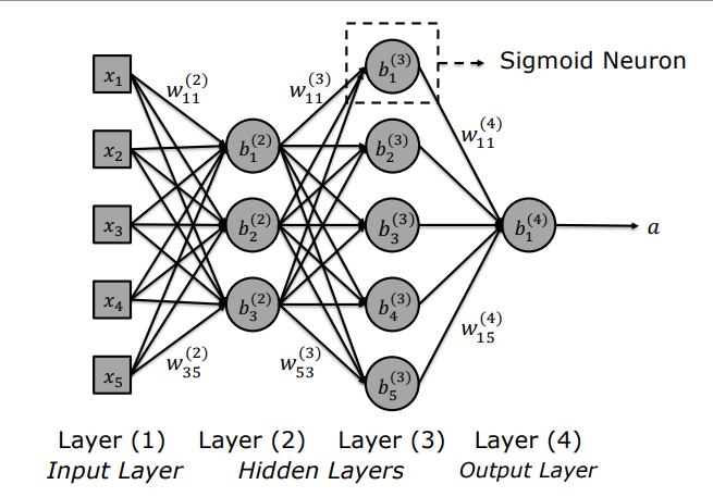
1.2 Michael Nielsen’s MNIST Classifier Case Study
Michael Nielsen’s canonical handwritten digit classification network demonstrates this layered configuration:
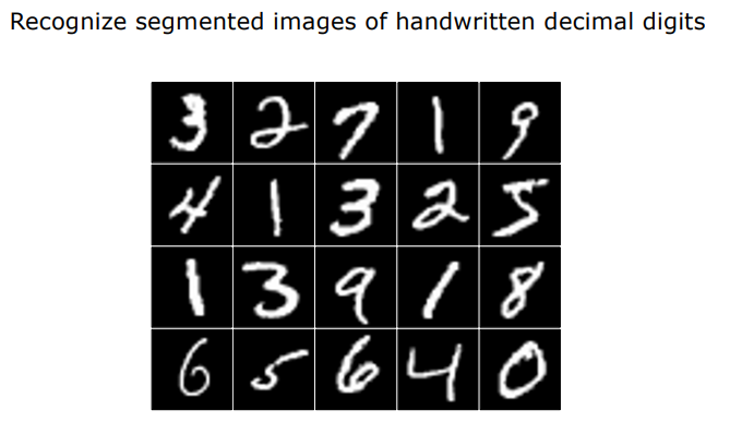
- Input Layer: 784 neurons ($28 \times 28$ normalized pixel brightness vector).
- Hidden Layer: 30 neurons (fully connected).
- Output Layer: 10 neurons (one activation for each digit class $0$ to $9$).
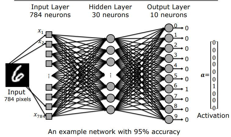
Parameter Count Breakdown:
- Weights:
- Layer 1 to Layer 2: $784 \times 30 = 23,520$ weights
- Layer 2 to Layer 3: $30 \times 10 = 300$ weights
- Total Weights: $23,520 + 300 = 23,820$
- Biases:
- Hidden Layer: $30$ biases
- Output Layer: $10$ biases
- Total Biases: $30 + 10 = 40$
- Total Trainable Parameters: $$\text{Total Parameters} = 23,820 + 40 = 23,860$$
2. Cost Function and Gradient Descent
A newly initialized network with random weights produces arbitrary, uncalibrated activations. Training the network entails adjusting parameters to minimize discrepancy between predicted outputs and ground-truth labels.
2.1 Desired Activations and the Mean Squared Error (MSE) Cost
For each training image $x$, ground-truth class labels are represented as one-hot encoded target vectors $\hat{\mathbf{a}}(x)$:
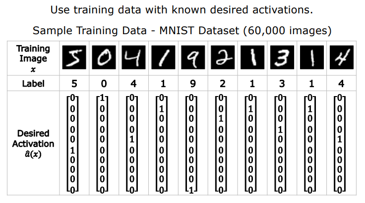
Prior to training, random initialization yields noisy output distributions far from ground truth:
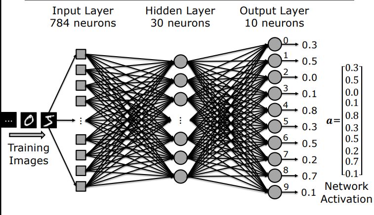
Mean Squared Error (MSE) Cost Formulation:
For an individual training sample $x$, the quadratic cost $C_x$ measures the squared Euclidean distance between network activations $\mathbf{a}(x)$ and target vector $\hat{\mathbf{a}}(x)$:
$$C_x(\mathbf{w}, \mathbf{b}) = |\hat{\mathbf{a}}(x) - \mathbf{a}(x | \mathbf{w}, \mathbf{b})|^2 = \sum_{j} \left( \hat{a}_j(x) - a_j^L(x) \right)^2$$
Averaged across the full training dataset ($n = 60,000$ images):
$$C(\mathbf{w}, \mathbf{b}) = \frac{1}{n} \sum_{x} C_x(\mathbf{w}, \mathbf{b})$$
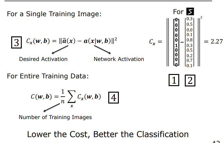
flowchart LR
Init["1. Initialize Weights & Biases\nwith Random Values"] --> Forward["2. Forward Propagate Inputs\nCompute Network Activations a(x)"]
Forward --> Cost["3. Evaluate Mean Squared Error\nCost Function C(w,b)"]
Cost --> Opt["4. Gradient Descent Optimization\nUpdate Weights & Biases"]
Opt --> Forward
style Init fill:#1a1a2e,stroke:#e94560,color:#fff
style Forward fill:#16213e,stroke:#4cc9f0,color:#fff
style Cost fill:#0f3460,stroke:#e94560,color:#fff
style Opt fill:#53354a,stroke:#e94560,color:#fff
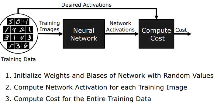
2.2 Mathematics of Gradient Descent and the Error Surface
The objective is to locate the global or near-optimal local minimum on the 23,860-dimensional cost surface $C(\mathbf{w}, \mathbf{b})$.
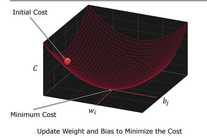
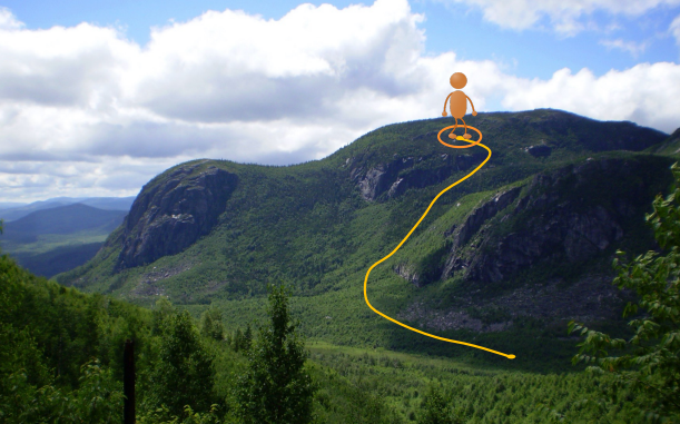
Analytical Steepest Descent Derivation:
A differential parameter displacement $\Delta \mathbf{v} = [\Delta w_1, \dots, \Delta b_1, \dots]^T$ induces a first-order change in cost $\Delta C$:
$$\Delta C \approx \nabla C \cdot \Delta \mathbf{v}$$
Where $\nabla C$ is the gradient vector of partial derivatives:
$$\nabla C = \left[ \frac{\partial C}{\partial w_1}, \frac{\partial C}{\partial w_2}, \dots, \frac{\partial C}{\partial b_1}, \dots \right]^T$$
To enforce maximal decrease ($\Delta C < 0$), Cauchy-Schwarz inequality dictates selecting $\Delta \mathbf{v}$ antiparallel to $\nabla C$:
$$\Delta \mathbf{v} = -\eta \nabla C$$
Where $\eta > 0$ is the Learning Rate. Substituting this yields:
$$\Delta C \approx \nabla C \cdot (-\eta \nabla C) = -\eta |\nabla C|^2 \leq 0$$
Because $-\eta |\nabla C|^2$ is strictly non-positive, every gradient descent update step guarantees reducing or maintaining the objective loss!
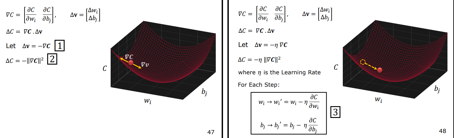
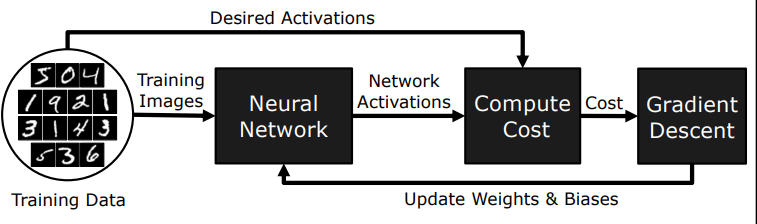
Parameter Update Equations:
$$w_i \leftarrow w_i - \eta \frac{\partial C}{\partial w_i}$$ $$b_j \leftarrow b_j - \eta \frac{\partial C}{\partial b_j}$$
2.3 Computational Collapse of Brute-Force Finite Differences
To execute gradient descent, we must evaluate $23,860$ partial derivatives at every iteration.
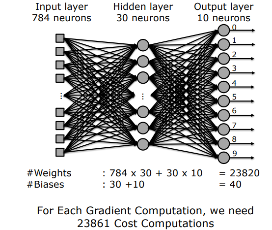
Using the standard numerical Finite Differences approximation:
$$\frac{\partial C}{\partial w_k} \approx \frac{C(\mathbf{w} + \epsilon \mathbf{e}_k, \mathbf{b}) - C(\mathbf{w}, \mathbf{b})}{\epsilon}$$
Workload Quantification:
- One image forward pass: $23,820$ multiplications.
- Dataset evaluation ($60,000$ images) for one loss calculation $C(\mathbf{w}, \mathbf{b})$: $$60,000 \times 23,820 \approx 1.43 \times 10^9 \text{ multiplications}$$
- Perturbing $23,860$ parameters individually requires evaluating the dataset 23,861 times: $$\text{Workload for 1 Gradient Step} = 23,861 \times (1.43 \times 10^9) \approx \mathbf{3.4 \times 10^{13}} \text{ multiplications!}$$
Critical Bottleneck: On supercomputers executing billions of operations per second, a single step would take days. Brute-force numerical differentiation is completely intractable for deep learning.
3. The Backpropagation Algorithm
The breakthrough that unlocked scalable neural network training is the Backpropagation Algorithm, which slashes gradient computation time by a factor of $10,000$.
3.1 Analytical Derivation via the Chain Rule
Backpropagation computes exact analytical derivatives in a single backward sweep using calculus chain rule. Let us derive the partial derivative for an output layer weight $w_{11}^{(4)}$:
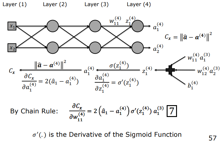
Applying the chain rule:
$$\frac{\partial C_x}{\partial w_{ji}^L} = \frac{\partial C_x}{\partial a_j^L} \cdot \frac{\partial a_j^L}{\partial z_j^L} \cdot \frac{\partial z_j^L}{\partial w_{ji}^L}$$
Evaluating each factor analytically:
- Loss with respect to Activation: $$C_x = \sum_k (a_k^L - \hat{a}_k)^2 \implies \frac{\partial C_x}{\partial a_j^L} = 2(a_j^L - \hat{a}_j)$$
- Activation with respect to Net Input (Sigmoid Derivative): $$a_j^L = \sigma(z_j^L) \implies \frac{\partial a_j^L}{\partial z_j^L} = \sigma’(z_j^L) = \sigma(z_j^L)(1 - \sigma(z_j^L)) = a_j^L (1 - a_j^L)$$
- Net Input with respect to Weight: $$z_j^L = \sum_k w_{jk}^L a_k^{L-1} + b_j^L \implies \frac{\partial z_j^L}{\partial w_{ji}^L} = a_i^{L-1}$$
Combining these terms:
$$\frac{\partial C_x}{\partial w_{ji}^L} = \underbrace{\left[ 2(a_j^L - \hat{a}j) \cdot a_j^L (1 - a_j^L) \right]}{\text{Local Gradient } \delta_j^L} \cdot a_i^{L-1}$$
3.2 Local Gradient ($\delta$) Formulation
The bracketed term defines the Local Gradient ($\delta_j^L$) of unit $j$ in layer $L$:
$$\delta_j^L = \frac{\partial C_x}{\partial z_j^L} = 2(a_j^L - \hat{a}_j) \cdot a_j^L (1 - a_j^L)$$
This reduces all parameter derivatives into modular two-factor products:
$$\frac{\partial C_x}{\partial w_{jk}^{(l)}} = \delta_j^{(l)} a_k^{(l-1)}$$ $$\frac{\partial C_x}{\partial b_j^{(l)}} = \delta_j^{(l)}$$
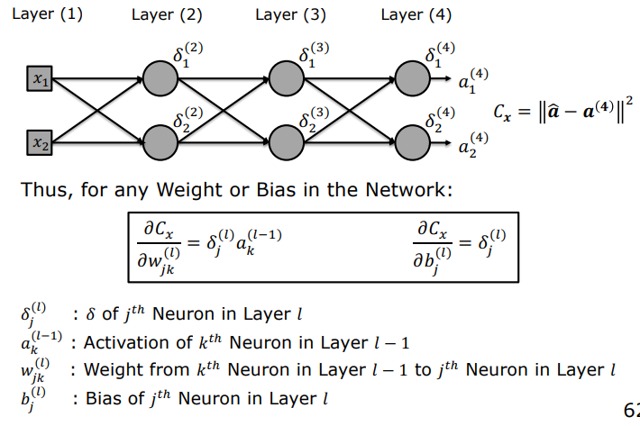
Backward Propagation of Errors to Hidden Layers:
Given downstream errors $\delta^{l+1}$, the error $\delta^l$ at hidden layer $l$ propagates backward through the transpose weight matrix:
$$\delta_j^l = \left( \sum_k \delta_k^{l+1} w_{kj}^{l+1} \right) a_j^l (1 - a_j^l)$$
flowchart RL
subgraph BackpropFlow["Error & Gradient Flow (Backward)"]
DL["Output Errors: δ^(L)"] -->|"Matrix Product (W^(L))^T"| DL1["Hidden Errors: δ^(L-1)"]
DL1 -->|"Matrix Product (W^(L-1))^T"| DL2["Prior Hidden Errors: δ^(2)"]
end
style DL fill:#e94560,stroke:#fff,color:#fff
style DL1 fill:#0f3460,stroke:#4cc9f0,color:#fff
style DL2 fill:#16213e,stroke:#4cc9f0,color:#fff
3.3 Complexity Comparison Matrix
| Optimization Method | Multiplications per Sample | Total Workload for 60,000 Images (1 Iteration) | Relative Speedup |
|---|---|---|---|
| Finite Differences | $23,861 \times 23,820 \approx 5.68 \times 10^8$ | $\mathbf{3.4 \times 10^{13}} \text{ operations}$ | $1\times$ (Baseline - Intractable) |
| Backpropagation | $23,820 \text{ (Forward)} + 24,210 \text{ (Backward)} = 48,030$ | $\mathbf{2.8 \times 10^9} \text{ operations}$ | $\mathbf{\approx 10,000\times \text{ Faster!}}$ |
Summary: Backpropagation slashes gradient complexity by 4 orders of magnitude ($10^4$), turning impossible multi-day computations into sub-second matrix passes.
4. Example Applications in Computer Vision
4.1 Handwritten Digit Recognition (MNIST)
Trained MLPs correctly classify heavily stylized and noisy digits with high confidence:
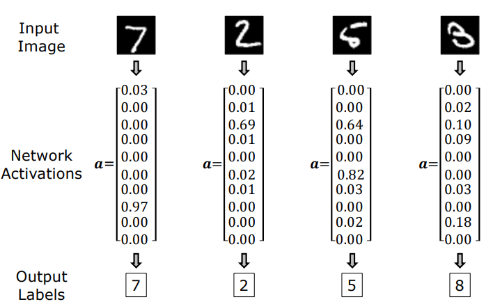
4.2 Convolutional Neural Networks (LeNet / CNNs)
In early computer vision, spatial feature extractors (e.g., Sobel or Gaussian filters) were handcrafted. In Yann LeCun’s (1998) Convolutional Neural Networks:
- Kernel filter coefficients ($k_1 \dots k_5$) serve as trainable network weights.
- Backpropagation automatically learns optimal spatial visual filters tailored to the visual task.
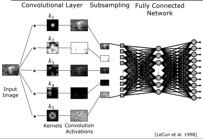
4.3 Multi-Label Semantic Tagging (Clarifai)
Modern deep networks extract rich multi-concept descriptors from unconstrained visual scenes:
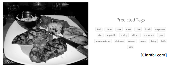
5. When to Use Machine Learning?
While deep neural networks are remarkably versatile, applying machine learning to phenomena governed by well-known physical laws introduces unnecessary computational overhead and opacity.
5.1 First Principles vs. Data-Driven ML
Consider calculating the displacement $s$ of a falling body over time $t$:
- First Principles (Newtonian Physics): $$s = ut + \frac{1}{2}at^2$$ Requires zero training data, evaluates instantly, and delivers foundational physical insight ($a = \text{gravity}$).
- Data-Driven ML: Dropping hundreds of balls, logging noisy time records, and fitting thousands of parameters with stochastic gradient descent.
Drawbacks of Pure ML in Closed-Physics Regimes:
- Computational & Resource Inefficiency: Massive data collection and GPU cycles are wasted relearning a known exact formula.
- Zero Scientific Insight (Black-Box): The network models input-output correlation without conveying physical understanding of gravitational mechanics.
- The Last Mile Problem: Pure data models reach $90-95%$ accuracy quickly, but attaining the $99.99%$ reliability required by safety-critical vision systems demands increasingly prohibitive data collection.
5.2 Decision Matrix: First Principles vs. Machine Learning
| Decision Dimension | First Principles (Analytical / Physics) | Machine Learning (Data-Driven) |
|---|---|---|
| Process Determinism | Governed by well-defined optical and geometric laws (perspective projection, photometric stereo, camera calibration). | The underlying process exhibits extreme stochastic variation or intractable complexity (handwriting, general faces). |
| Explainability | Fully transparent, mathematically provable, and physically interpretable. | Opaque black-box; decisions emerge from millions of distributed weight interactions. |
| Data Requirement | Zero training data; analytical formulas execute immediately. | Requires thousands or millions of cleaned, annotated training samples. |
| Computational Footprint | Lightweight, runs deterministically on standard CPUs. | Demands intensive GPU/TPU training clusters and long convergence runs. |
Golden Engineering Rule (Symbiotic Coexistence): The most robust computer vision systems leverage first principles as far as analytical modeling permits, and transition to machine learning precisely where hand-crafted physical rules reach their descriptive limit.
Content
Deep Learning with PyTorch
Comprehensive Notes on Deep Learning, Tensor Internals, Computer Vision, Transformers, and Production Deployment
∴
These notes document a systematic, first-principles study of Deep Learning with PyTorch (2nd Edition, Manning) by Eli Stevens, Luca Antiga, Thomas Viehmann, and Howard Huang.
Manning Publications
Luca Antiga, Eli Stevens, Thomas Viehmann, Howard Huang
Book & Note Structure
| Part | Focus & Scope | Core Contents |
|---|---|---|
| Part 1: Core PyTorch | Framework Mechanics & Low-Level Foundations | Tensors, physical 1D storage buffers, strides, autograd DAG engine, modular nn.Module design, datasets/dataloaders, and 2D/3D convolutions. |
| Part 2: Practical Applications | Advanced Vision, NLP & Systems Engineering | Vision Transformers (ViT), Diffusion Models (DDPM), 3D Volumetric CT Scan Cancer Detection, SAM Fine-Tuning, Multi-GPU Parallelisms (FSDP/TP/PP), and Production Deployment (torch.compile, LibTorch C++, ExecuTorch). |
— emreaslan —
Introducing Deep Learning and the PyTorch Library
- 1. What is Deep Learning?
- 2. The Shift from Machine Learning to Deep Learning
- 3. What is a Tensor?
- 4. Why PyTorch?
- 5. The Anatomy of a Deep Learning Project
- 6. Verifying Your Installation and Hardware Setup
- 7. Summary and Key Takeaways

Welcome to the world of deep learning with PyTorch. If you have ever wondered how computers can recognize faces in photos, translate spoken sentences in real time, or generate realistic images from text prompts, deep learning is the technology behind these breakthroughs.
This chapter introduces the fundamental concepts of deep learning from the ground up. You will learn what deep learning is, how it differs from traditional machine learning, what a tensor is in simple terms, why PyTorch has become the primary tool for researchers and engineers worldwide, and how a typical deep learning project is structured.
1. What is Deep Learning?
For decades, traditional computer programs were written using explicit, handcrafted rules. A human programmer would write logic: “If temperature is above 30 and humidity is high, turn on the air conditioner.”
However, for complex real-world tasks like identifying a pedestrian in a camera feed or understanding a spoken language, writing manual rules is practically impossible. There are simply too many variations in lighting, pose, clothing, and accents.
flowchart LR
subgraph Traditional["Traditional Programming"]
D1["Data"] & R1["Handwritten Rules"] --> P1["Computer"] --> O1["Output"]
end
subgraph MachineLearning["Machine Learning / Deep Learning"]
D2["Data"] & O2["Target Answers"] --> P2["Learning Algorithm"] --> R2["Learned Rules / Model"]
end
style Traditional fill:#1a1a2e,stroke:#e94560,color:#fff
style MachineLearning fill:#16213e,stroke:#4cc9f0,color:#fff
Deep learning flips the traditional programming paradigm. Instead of writing rules by hand, we feed the computer thousands of examples (inputs and their correct answers), and the computer learns the mathematical rules automatically.
As the computer scientist Edsger W. Dijkstra famously observed:
“The question of whether machines can think is about as relevant as whether submarines can swim.”
In deep learning, we do not need machines to have human consciousness; we simply need them to reliably approximate complex functions that map inputs to outputs.
2. The Shift from Machine Learning to Deep Learning
To understand why deep learning revolutionized artificial intelligence, we must look at how classical machine learning handled data compared to deep learning.
flowchart TD
subgraph Classical["Classical Machine Learning (Handcrafted Features)"]
C1["Raw Image (Pixels)"] --> C2["Human Feature Engineering\n(Edge Detectors, Texture Histograms, SIFT)"]
C2 --> C3["Shallow Classifier\n(Logistic Regression, SVM)"]
C3 --> C4["Prediction: 'Dog'"]
end
subgraph Modern["Deep Learning (End-to-End Representation Learning)"]
M1["Raw Image (Pixels)"] --> M2["Layer 1: Low-Level (Edges & Spots)"]
M2 --> M3["Layer 2: Mid-Level (Corners & Textures)"]
M3 --> M4["Layer 3: High-Level (Eyes, Ears, Noses)"]
M4 --> M5["Prediction: 'Dog'"]
end
style Classical fill:#1a1a2e,stroke:#e94560,color:#fff
style Modern fill:#0f3460,stroke:#00b4d8,color:#fff
2.1 The Bottleneck of Feature Engineering
In classical machine learning, the machine learning algorithm itself (such as a Support Vector Machine or Linear Regression) cannot process raw pixel grids directly with high accuracy. A human engineer had to spend weeks manually extracting “features”:
- Computing color histograms
- Designing edge filters
- Extracting corner descriptors (like SIFT or Harris corners)
If the human designed poor features, the model failed. The performance was fundamentally limited by human domain expertise.
2.2 Hierarchical Representation Learning
Deep learning replaces manual feature engineering with layered representations. A deep neural network is composed of successive layers of artificial neurons. Each layer takes the output of the previous layer and transforms it:
- First Layers: Learn simple geometrical primitives, such as oriented lines, color boundaries, and brightness gradients.
- Middle Layers: Combine edges to detect textures, corners, contours, and basic shapes (circles, stripes).
- Deeper Layers: Combine shapes to detect semantic components (eyes, wheels, dog ears, door handles).
- Final Layer: Combines object parts to produce the final classification decision.
Because every layer is differentiable, the entire hierarchy is optimized simultaneously through gradient descent.
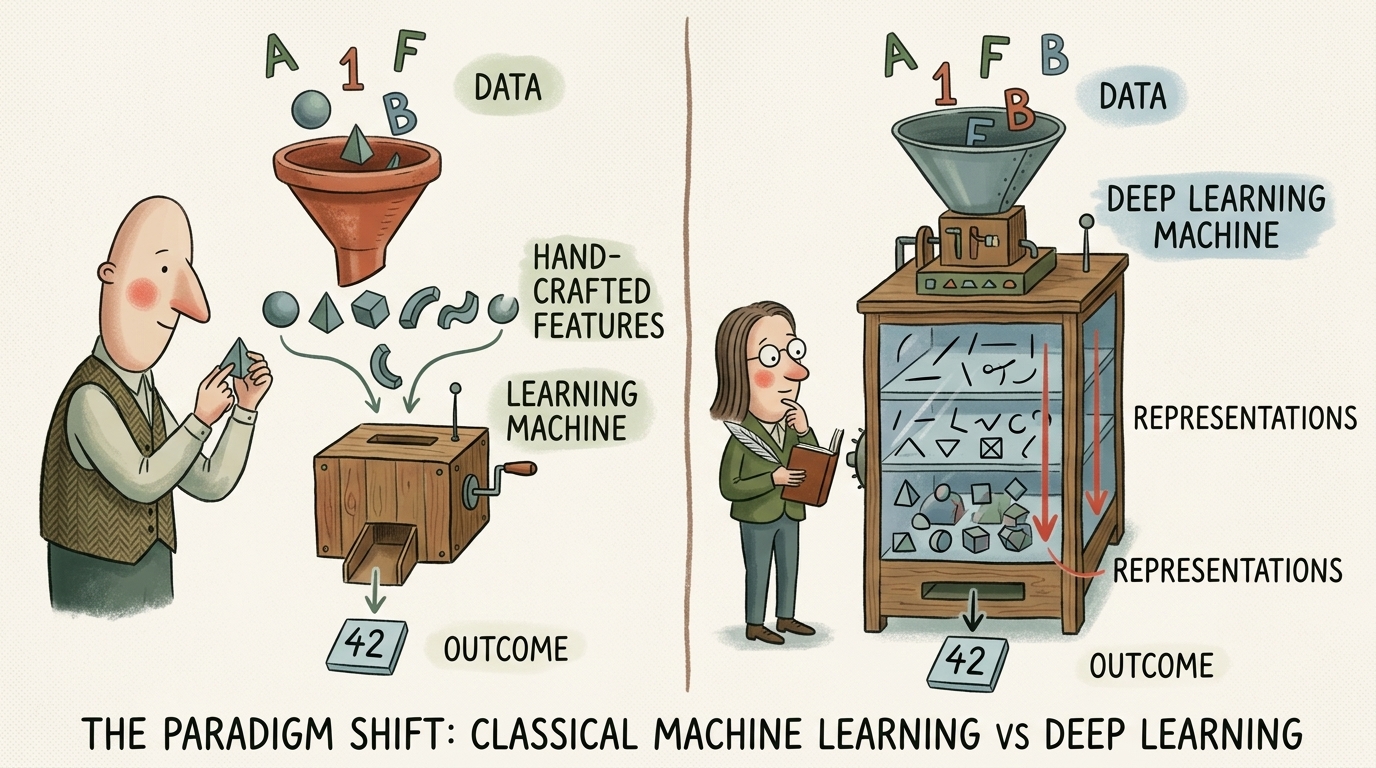
3. What is a Tensor?
To work with PyTorch, you need to understand its fundamental data structure: the Tensor.
At first, the word tensor may sound intimidating. But in computer science, a tensor is simply a generalization of numbers, vectors, and matrices to any number of dimensions:
Dimension 0 (Scalar): 42
Dimension 1 (Vector): [1.0, 2.5, 3.8]
Dimension 2 (Matrix): [[1, 2],
[3, 4]]
Dimension 3 (3D Tensor): Array with Depth, Height, Width (e.g., Color Image)
Dimension 4 (4D Tensor): Batch of Images or a Video (Batch, Channels, Height, Width)
flowchart LR
S["Scalar (0D)\nSingle Number\ne.g. Temperature = 24.5"] --> V["Vector (1D)\nList of Numbers\ne.g. Audio samples [x1, x2, x3]"]
V --> M["Matrix (2D)\nTable of Numbers\ne.g. Grayscale image (H x W)"]
M --> T["Tensor (3D / 4D / ND)\nMultidimensional Grid\ne.g. RGB Image (3 x H x W)\nVideo (Batch x Time x C x H x W)"]
style S fill:#1a1a2e,stroke:#e94560,color:#fff
style V fill:#16213e,stroke:#4cc9f0,color:#fff
style M fill:#0f3460,stroke:#e94560,color:#fff
style T fill:#1b262c,stroke:#00b4d8,color:#fff
3.1 Executable PyTorch Example: Creating Tensors
Here is an interactive Python script demonstrating how simple it is to create and inspect tensors in PyTorch:
import torch
# 1. Scalar (0-dimensional tensor)
scalar = torch.tensor(42.0)
print("Scalar:", scalar)
print("Scalar dimension (ndim):", scalar.ndim)
# 2. Vector (1-dimensional tensor)
vector = torch.tensor([1.5, 3.0, 4.5])
print("\nVector:", vector)
print("Vector shape:", vector.shape)
# 3. Matrix (2-dimensional tensor: 2 rows, 3 columns)
matrix = torch.tensor([[1, 2, 3],
[4, 5, 6]], dtype=torch.float32)
print("\nMatrix:\n", matrix)
print("Matrix shape (Rows, Columns):", matrix.shape)
# 4. 3D Tensor representing a small 3-channel (RGB) image (3 x 2 x 2)
rgb_image = torch.zeros((3, 2, 2))
print("\n3D Tensor (Channels x Height x Width) shape:", rgb_image.shape)
4. Why PyTorch?
PyTorch was created by researchers at Meta AI (formerly Facebook AI Research) and open-sourced in 2017. In just a few years, it became the undisputed standard framework for academic research and production AI.
What makes PyTorch special?
4.1 Pythonic and Intuitive (Eager Execution)
In early deep learning frameworks (like TensorFlow 1.x), writing code required two separate stages: first defining an abstract “symbolic graph”, and then running that graph inside a “session”. If your code crashed, the error message pointed to internal graph engines rather than your Python lines.
PyTorch introduced Eager Mode (Define-by-Run):
- PyTorch code executes immediately line by line, exactly like standard Python and NumPy.
- You can print tensor values at any time using
print(). - You can use regular Python
forloops,ifstatements, and standard debuggers (pdb).
import torch
# Dynamic control flow in pure Python
x = torch.tensor([2.0, -3.0, 5.0])
for val in x:
if val > 0:
print(f"Positive value detected: {val.item()}")
else:
print(f"Negative value detected: {val.item()}")
4.2 Seamless GPU Acceleration
PyTorch makes running computations on NVIDIA GPUs as simple as calling .to("cuda") or .to(device):
import torch
# Check if an NVIDIA CUDA GPU is available
device = "cuda" if torch.cuda.is_available() else "cpu"
print(f"Using device: {device}")
# Create two matrices and multiply them on the target device
a = torch.randn(1000, 1000, device=device)
b = torch.randn(1000, 1000, device=device)
c = torch.matmul(a, b)
print(f"Matrix multiplication result shape on {device}: {c.shape}")
4.3 The Bridge to Production: torch.compile in PyTorch 2.x
In modern PyTorch 2.0 and later, you no longer have to choose between dynamic research flexibility and static production speed. Adding a single line torch.compile(model) automatically optimizes and fuses your operations into high-speed C++/Triton GPU kernels behind the scenes.
5. The Anatomy of a Deep Learning Project
Every deep learning application built with PyTorch follows a structured, 5-step lifecycle:
flowchart LR
D["1. Prepare Data\n(Files -> Tensors)"] --> M["2. Define Model\n(nn.Module Architecture)"]
M --> L["3. Compute Loss\n(Measure Prediction Error)"]
L --> O["4. Optimize Parameters\n(Gradient Descent)"]
O --> S["5. Deploy to Production\n(Web, Server, Mobile)"]
style D fill:#1a1a2e,stroke:#e94560,color:#fff
style M fill:#16213e,stroke:#4cc9f0,color:#fff
style L fill:#0f3460,stroke:#e94560,color:#fff
style O fill:#1b262c,stroke:#00b4d8,color:#fff
style S fill:#2b2d42,stroke:#52b788,color:#fff
- Data Ingestion (
Dataset&DataLoader): Raw files (images, audio, text, CT scans) on disk are loaded, converted into numeric tensors, normalized, and grouped into mini-batches. - Model Definition (
nn.Module): We define the neural network architecture by connecting mathematical layers (linear projections, convolutions, attention blocks). - Loss Function (Criterion): We evaluate model predictions against ground-truth labels using a loss function (such as Mean Squared Error or Cross-Entropy Loss) that outputs a single numerical penalty score.
- Optimization Loop (Autograd & Optimizer): The optimizer (such as SGD or AdamW) calculates gradients via PyTorch’s automatic differentiation engine (
autograd) and slightly adjusts the model parameters to reduce the loss. - Deployment: The trained model is saved, exported (via ONNX, LibTorch, or
torch.export), and served via an API server (FastAPI) or deployed on edge devices (mobile phones, embedded cameras).
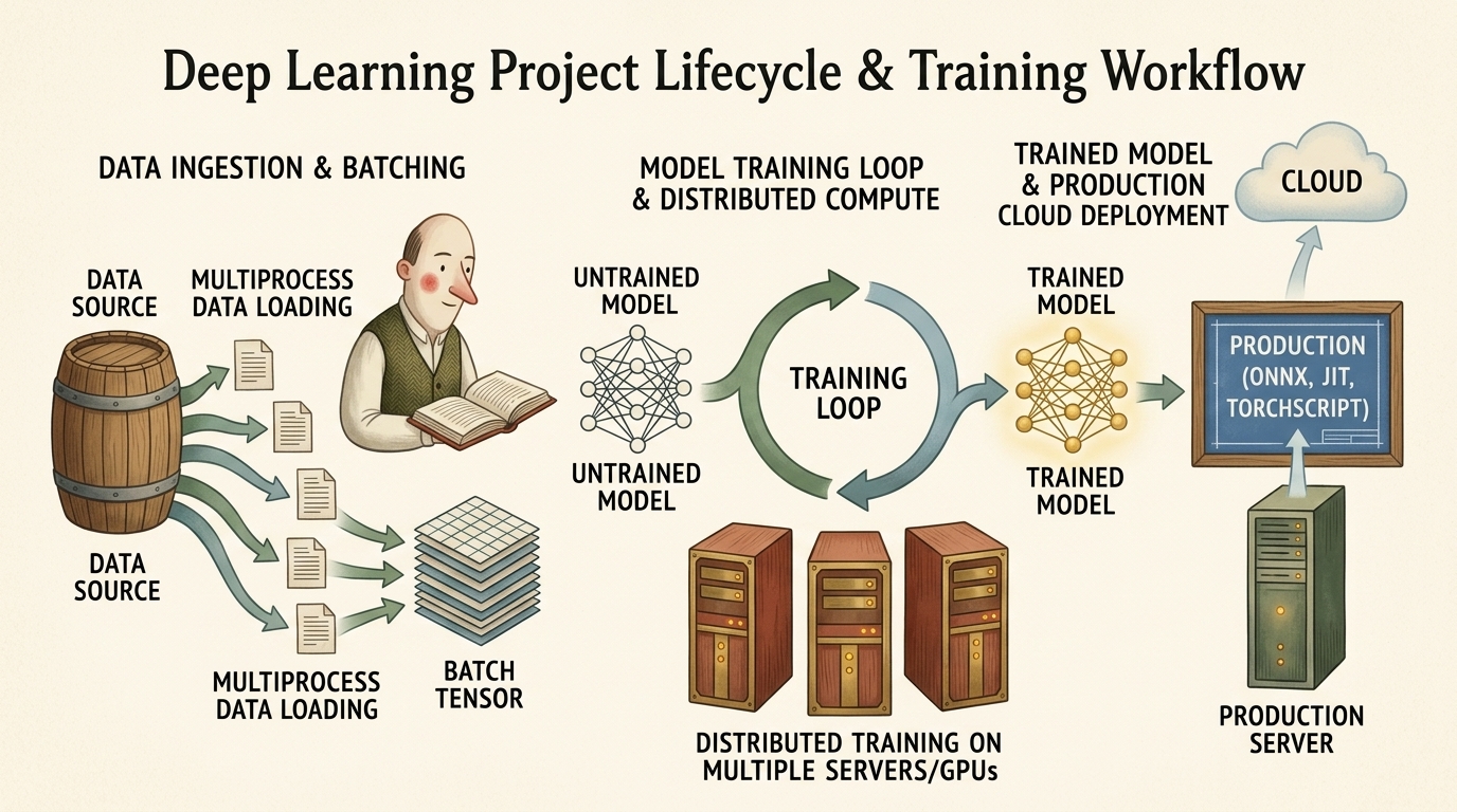
6. Verifying Your Installation and Hardware Setup
To follow along with the exercises and practical code in this book, run the following diagnostic script in your Python environment or Jupyter Notebook:
import sys
import torch
print("=== System and PyTorch Diagnostics ===")
print(f"Python Version: {sys.version.split()[0]}")
print(f"PyTorch Version: {torch.__version__}")
# GPU Availability
cuda_available = torch.cuda.is_available()
print(f"CUDA Available: {cuda_available}")
if cuda_available:
device_count = torch.cuda.device_count()
device_name = torch.cuda.get_device_name(0)
print(f"Number of GPUs: {device_count}")
print(f"Primary GPU Device Name: {device_name}")
else:
print("Running on CPU mode. Standard training in Part 1 will run fine.")
print("PyTorch environment successfully verified!")
7. Summary and Key Takeaways
- Deep Learning vs. Classical ML: Classical machine learning relies on human feature engineering. Deep learning automatically learns hierarchical, layered representations directly from raw data.
- Tensors: Tensors are multidimensional arrays of numbers (scalars, vectors, matrices, 3D/4D grids) and serve as the universal language of PyTorch.
- Eager Execution: PyTorch executes code dynamically line by line, making model construction, debugging, and experimentation natural and intuitive.
- The Core Project Loop: Deep learning projects follow a repeatable pattern: Data Loading $\to$ Model Architecture $\to$ Loss Calculation $\to$ Backpropagation Optimization $\to$ Deployment.
Pretrained Networks and the Model Zoo
- 1. The Pretrained Foundation Model Paradigm
- 2. Image Recognition: Torchvision Model Zoo
- 3. Generative Vision Pipelines: Inpainting & CycleGAN
- 4. The Hugging Face Ecosystem & Model Zoo
- 5. Vision-Language Multimodal Inference: BLIP
- 6. Model Sizing, Computational Complexity (FLOPs) & GPU VRAM
- 7. Summary and Key Takeaways
Training modern deep neural networks from scratch on web-scale datasets like ImageNet (1.2 million labeled images across 1,000 classes) or LAION requires hundreds of GPU hours, massive compute clusters, and substantial engineering budgets. In modern production machine learning, engineers rarely start from random parameter initializations ($W \sim \mathcal{N}(0, \sigma^2)$). Instead, they build upon pretrained foundation networks that have already learned high-capacity visual and multimodal representations.
This chapter walks step-by-step through the core pretrained models covered in Chapter 2 of Deep Learning with PyTorch (2nd Edition):
- Visual Recognition: Classic CNNs (AlexNet, ResNet-101) and modern Vision Transformers (ViT).
- Generative Image Synthesis: Text-conditioned inpainting with Latent Diffusion (Stable Diffusion) and unpaired image translation with CycleGAN (Horse $\to$ Zebra).
- The Hugging Face Ecosystem: Universal model repositories and standardized processor/model interfaces.
- Multimodal Vision-Language: Scene understanding and automated image captioning with BLIP.
1. The Pretrained Foundation Model Paradigm
In classical software engineering, developers reuse vetted libraries for encryption or database operations rather than reimplementing algorithms from scratch. Pretrained deep neural networks provide the exact same modularity for artificial intelligence:
flowchart LR
subgraph Pretraining["1. Web-Scale Upstream Pretraining"]
D["Massive Dataset\n(ImageNet / LAION / Common Crawl)"] --> T["Compute Cluster\n(Weeks of Gradient Descent)"]
T --> BB["Pretrained Backbone Weights\n(Universal Spatial & Semantic Features)"]
end
subgraph Downstream["2. Downstream Tasks & Inference"]
BB --> CLF["Direct Inference / Zero-Shot\n(Classification, VQA, Captioning)"]
BB --> FT["Transfer Learning & Fine-Tuning\n(Medical Imaging, Robotics, Edge AI)"]
end
style Pretraining fill:#1a1a2e,stroke:#e94560,color:#fff
style Downstream fill:#16213e,stroke:#4cc9f0,color:#fff
style BB fill:#0f3460,stroke:#00b4d8,color:#fff
The ImageNet Benchmark and Visual Hierarchy
The canonical benchmark for computer vision is ImageNet, organized according to the WordNet lexical noun hierarchy. ImageNet contains over 14 million images, with its primary competition subset (ILSVRC) featuring 1,000 distinct object categories (e.g., dog breeds, vehicles, everyday tools).
When a network learns to discriminate across these 1,000 classes, its internal layers build a hierarchical visual vocabulary:
- Early layers: Detect low-level spatial primitives (Gabor-like edges, color contrasts, line orientations).
- Middle layers: Assemble edges into textures, surface curvatures, corners, and contours.
- Deep layers: Compose textures into complex semantic entities (eyes, snouts, wheels, object assemblies).
Key Insight: Pretrained weights freeze thousands of GPU hours of gradient descent optimization into physical tensor checkpoints. Loading these weights gives your model immediate high-level visual and semantic perception capabilities.
2. Image Recognition: Torchvision Model Zoo
The torchvision.models subpackage provides instant access to vetted computer vision architectures and their pretrained weights.
flowchart TD
HUB["torchvision.models"] --> CLF["Image Classification"]
CLF --> C1["AlexNet (2012 Historical Baseline)"]
CLF --> C2["ResNet-18 / ResNet-101 (Residual CNNs)"]
CLF --> C3["ViT-B/16 (Vision Transformer)"]
style HUB fill:#1a1a2e,stroke:#e94560,color:#fff
style CLF fill:#16213e,stroke:#4cc9f0,color:#fff
style C1 fill:#0f3460,stroke:#e94560,color:#fff
style C2 fill:#1b262c,stroke:#00b4d8,color:#fff
style C3 fill:#2b2d42,stroke:#52b788,color:#fff
2.1 Inspecting Available Architectures
Before instantiating a model, we can query all available models in the Torchvision catalog using models.list_models().
import torch
import torchvision
from torchvision import models
# List all available models in torchvision
available_models = models.list_models()
print(f"Total available models in Torchvision: {len(available_models)}")
print("Sample models:", available_models[:10])
2.2 AlexNet: The 2012 Deep Learning Revolution
AlexNet (Krizhevsky, Sutskever, & Hinton, 2012) triggered the modern deep learning boom by winning the ILSVRC 2012 competition, slashing the top-5 error rate from 28.2% (classical feature extraction methods like SIFT/HOG) to 16.4%.
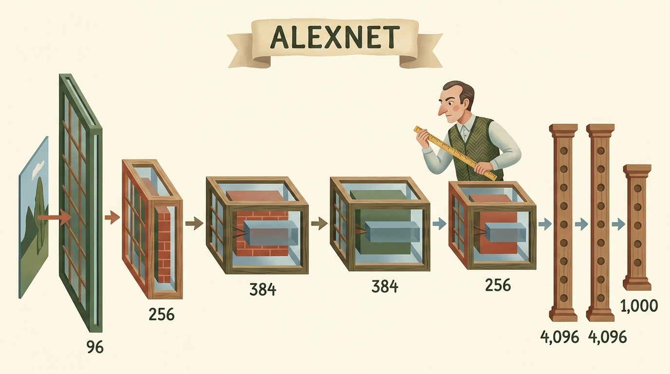
AlexNet contains 61.1 million parameters across 5 convolutional layers and 3 fully connected layers.
Step 1: Instantiating AlexNet with Weights
In modern Torchvision (v0.13+), models are loaded using explicit Weights enum objects rather than legacy boolean flags (pretrained=True). This guarantees reproducibility and automatically bundles the exact preprocessing transformations used during training.
from torchvision.models import AlexNet_Weights
# Instantiate AlexNet with default pretrained ImageNet weights
alexnet_weights = AlexNet_Weights.DEFAULT
alexnet = models.alexnet(weights=alexnet_weights)
# Inspect network topology
print(alexnet)
The output reveals two main submodules:
features: A sequential cascade ofConv2d,ReLU, andMaxPool2dlayers that progressively downsample spatial resolution while expanding feature channels ($3 \to 64 \to 192 \to 384 \to 256$).classifier: Fully connected linear layers withDropout(p=0.5)ending withLinear(in_features=4096, out_features=1000)producing logits for each ImageNet category.
2.3 The Vision Transformer (ViT): Attention Replaces Convolution
In 2020, Dosovitskiy et al. introduced An Image is Worth 16x16 Words: Transformers for Image Recognition at Scale (ViT). ViT discards convolutional inductive biases (translational equivariance and local receptive fields) in favor of Self-Attention across flattened image patches.
flowchart TD
IMG["Input Image (3, 224, 224)"] --> PATCH["Extract 14x14 = 196 Patches\nEach Patch: (3, 16, 16) -> 768-d Vector"]
PATCH --> POS["Add Learnable Positional Embedding\n+ [CLS] Class Token Token_0"]
POS --> TR["12x Transformer Encoder Blocks\n(Multi-Head Self-Attention + MLP)"]
TR --> HEAD["MLP Classification Head\nExtract [CLS] Representation"]
HEAD --> OUT["1000 Class Logits"]
style IMG fill:#1a1a2e,stroke:#e94560,color:#fff
style PATCH fill:#16213e,stroke:#4cc9f0,color:#fff
style POS fill:#0f3460,stroke:#00b4d8,color:#fff
style TR fill:#1b262c,stroke:#52b788,color:#fff
style HEAD fill:#2b2d42,stroke:#52b788,color:#fff
style OUT fill:#343a40,stroke:#fca311,color:#fff
Step 1: Instantiating ViT-B/16
We load the Vision Transformer Base model with $16 \times 16$ patch resolution (vit_b_16):
from torchvision.models import ViT_B_16_Weights
# Instantiate ViT-B/16 with default pretrained weights
vit_weights = ViT_B_16_Weights.DEFAULT
vit = models.vit_b_16(weights=vit_weights)
# Inspect network topology
print(vit)
In vit_b_16, the $224 \times 224$ input is divided into $14 \times 14 = 196$ non-overlapping patches of size $16 \times 16 \times 3 = 768$ values. A learnable class token ([CLS]) is prepended to the sequence (making sequence length $197$), and $12$ Transformer encoder blocks process global dependencies via multi-head self-attention.
2.4 Mathematical Input Preprocessing Pipeline
Neural network weights are mathematically calibrated to the exact mean and variance of their training data. Feeding raw unnormalized RGB pixel values into a pretrained network causes severe distribution shift, resulting in random garbage outputs.
flowchart LR
RAW["Raw PIL Image\n(Arbitrary H x W)"] --> RES["Resize (Shortest Edge=256)\n& Center Crop (224x224)"]
RES --> TO_TENS["Convert to Tensor & Scale\n[0, 255] -> [0.0, 1.0]"]
TO_TENS --> NORM["Per-Channel Standardize\n(x - mean) / std"]
NORM --> UNSQ["Add Batch Dim via unsqueeze(0)\nShape: (1, 3, 224, 224)"]
style RAW fill:#1a1a2e,stroke:#e94560,color:#fff
style RES fill:#16213e,stroke:#4cc9f0,color:#fff
style TO_TENS fill:#0f3460,stroke:#e94560,color:#fff
style NORM fill:#1b262c,stroke:#00b4d8,color:#fff
style UNSQ fill:#2b2d42,stroke:#52b788,color:#fff
The mathematical transformation pipeline consists of four deterministic operations:
-
Spatial Rescaling & Central Cropping: The image is scaled so its shortest side is 256 pixels, followed by a central crop of size $224 \times 224$: $$ \mathbf{X} \in \mathbb{R}^{3 \times 224 \times 224} $$
-
Pixel Intensity Normalization: Integer byte values $x \in [0, 255]$ are mapped to floating-point numbers in $[0.0, 1.0]$: $$ x_{\text{norm}} = \frac{x}{255.0} $$
-
Per-Channel Standardization: Each RGB channel $c \in {0, 1, 2}$ is standardized using ImageNet dataset statistics: $$ x’_{c,i,j} = \frac{x_{c,i,j} - \mu_c}{\sigma_c} $$ $$ \boldsymbol{\mu} = [0.485, 0.456, 0.406], \quad \boldsymbol{\sigma} = [0.229, 0.224, 0.225] $$
Step 1: Retrieving the Official Preprocessing Transform
Instead of manually hardcoding normalization vectors, we retrieve the exact transformation pipeline bound to the model weights:
# Extract the official preprocessing pipeline
preprocess = alexnet_weights.transforms()
print("Preprocessing Pipeline Configuration:")
print(preprocess)
Step 2: Downloading a Real Test Image
We load the canonical Golden Retriever test photo directly from PyTorch’s official repository:
import urllib.request
from PIL import Image
# Download and open real test image
url = "https://raw.githubusercontent.com/pytorch/hub/master/images/dog.jpg"
with urllib.request.urlopen(url) as response:
img = Image.open(response).convert("RGB")
print(f"Original image format: {img.format}, dimensions: {img.size}")
Step 3: Applying Preprocessing Transformations
We apply the preprocessing pipeline to transform the PIL image into a standardized $(3, 224, 224)$ float tensor:
# Apply preprocessing transformations: PIL Image -> (3, 224, 224) Tensor
img_t = preprocess(img)
print(f"Preprocessed tensor shape: {img_t.shape}")
print(f"Tensor dtype: {img_t.dtype}, min: {img_t.min():.2f}, max: {img_t.max():.2f}")
Step 4: Adding Batch Dimension via unsqueeze(0)
PyTorch models expect a 4D tensor representing (Batch, Channels, Height, Width). We add the batch dimension using torch.unsqueeze(0):
import torch
# Add batch dimension: (3, 224, 224) -> (1, 3, 224, 224)
batch_t = torch.unsqueeze(img_t, 0)
print(f"Input batch tensor shape: {batch_t.shape}")
2.5 Running Inference and Decoding Class Probabilities
Step 1: Setting Evaluation Mode & Forward Pass
Before performing inference, we MUST set the model to evaluation mode using model.eval(). This freezes stochastic behavior in layers like Dropout and fixes running statistics in BatchNorm2d.
We wrap the forward pass inside with torch.inference_mode(): to disable autograd and memory version counter tracking:
# 1. Set model to evaluation mode
alexnet.eval()
# 2. Select target computation device
device = torch.device("cuda" if torch.cuda.is_available() else "cpu")
alexnet = alexnet.to(device)
batch_t = batch_t.to(device)
# 3. Perform forward pass
with torch.inference_mode():
out = alexnet(batch_t)
print(f"Output raw logits shape: {out.shape}") # (1, 1000)
Step 2: Softmax Normalization & Top-5 Extraction
The network outputs raw, unnormalized logits $\mathbf{z} \in \mathbb{R}^{1000}$. To convert logits into valid probabilities $P(Y = k) \in (0, 1)$ such that $\sum_k P(Y=k) = 1$, we apply the Softmax function:
$$ P(Y = k \mid \mathbf{x}) = \text{Softmax}(z_k) = \frac{\exp(z_k)}{\sum_{j=1}^{1000} \exp(z_j)} $$
We then extract the top-5 most confident class predictions using torch.topk:
# 1. Apply Softmax along class dimension (dim=1)
probabilities = torch.softmax(out, dim=1)
# 2. Extract top-5 predictions
top5_prob, top5_catid = torch.topk(probabilities, 5)
# 3. Retrieve category names from weights metadata
categories = alexnet_weights.meta["categories"]
print("\n=== AlexNet Top-5 Class Predictions for Golden Retriever ===")
for i in range(top5_prob.size(1)):
cat_id = top5_catid[0][i].item()
score = top5_prob[0][i].item() * 100.0
print(f"{i+1}. {categories[cat_id]:<35} ({score:.2f}%)")
Step 3: Comparative Inference with Vision Transformer (ViT-B/16)
Let’s run the exact same test image through ViT-B/16 to inspect how global self-attention compares with AlexNet:
vit.eval()
vit_preprocess = vit_weights.transforms()
vit_batch_t = torch.unsqueeze(vit_preprocess(img), 0).to(device)
with torch.inference_mode():
vit_out = vit(vit_batch_t)
vit_probs = torch.softmax(vit_out, dim=1)
vit_top5_prob, vit_top5_catid = torch.topk(vit_probs, 5)
vit_categories = vit_weights.meta["categories"]
print("=== ViT-B/16 Top-5 Class Predictions ===")
for i in range(vit_top5_prob.size(1)):
cat_id = vit_top5_catid[0][i].item()
score = vit_top5_prob[0][i].item() * 100.0
print(f"{i+1}. {vit_categories[cat_id]:<35} ({score:.2f}%)")
3. Generative Vision Pipelines: Inpainting & CycleGAN
While classification models learn discriminative boundaries ($P(Y \mid X)$), generative models learn the underlying data distribution to synthesize new realistic visual content ($P(X)$ or $P(X \mid \text{Prompt})$).
3.1 The Inpainting Process with Latent Diffusion Models (Stable Diffusion)
Generative inpainting restores, alters, or replaces masked sections of an image based on a natural language text prompt.
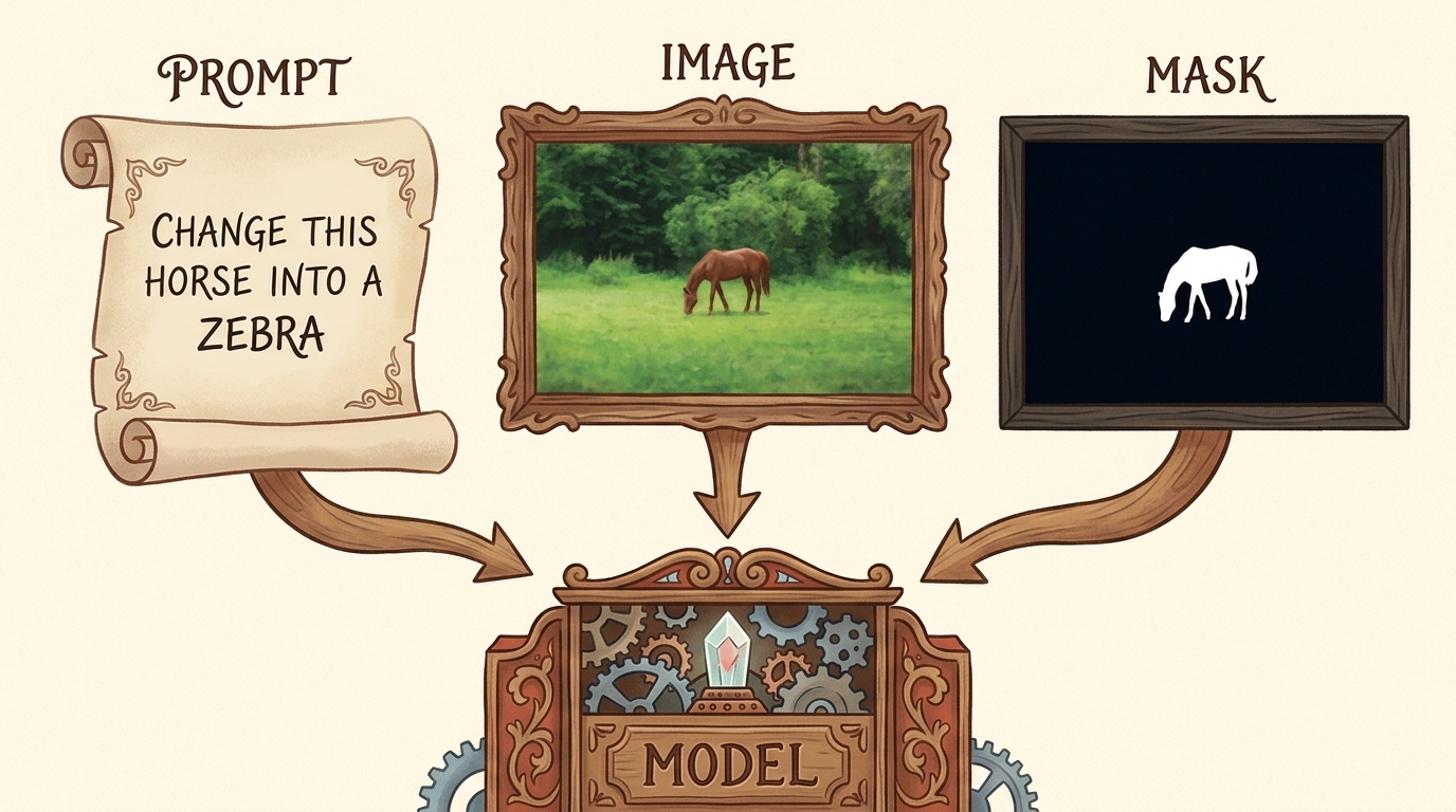
Why Latent Diffusion?
Standard diffusion models operate directly in high-dimensional pixel space ($512 \times 512 \times 3 = 786,432$ values), making multi-step denoising computationally prohibitive.
Latent Diffusion Models (LDMs) compress the image $8\times$ spatially into a lower-dimensional latent space $z = \mathcal{E}(x)$ of shape $(4, 64, 64) = 16,384$ values using a pretrained Variational Autoencoder (VAE). The denoising U-Net operates entirely in this compact latent manifold:
$$ \mathcal{L}_{\text{LDM}}(\theta) = \mathbb{E}_{\mathbf{x}, \mathbf{y}, \boldsymbol{\epsilon}, t} \left[ \left\| \boldsymbol{\epsilon} - \boldsymbol{\epsilon}_\theta(\mathbf{z}_t, t, \tau_\theta(\mathbf{y})) \right\|_2^2 \right] $$
Where:
- $\mathbf{z}_t$: Latent image at noise step $t$.
- $\tau_\theta(\mathbf{y})$: Conditioning text embedding from the CLIP text encoder.
- $\boldsymbol{\epsilon}_\theta$: U-Net predicting the noise perturbation.
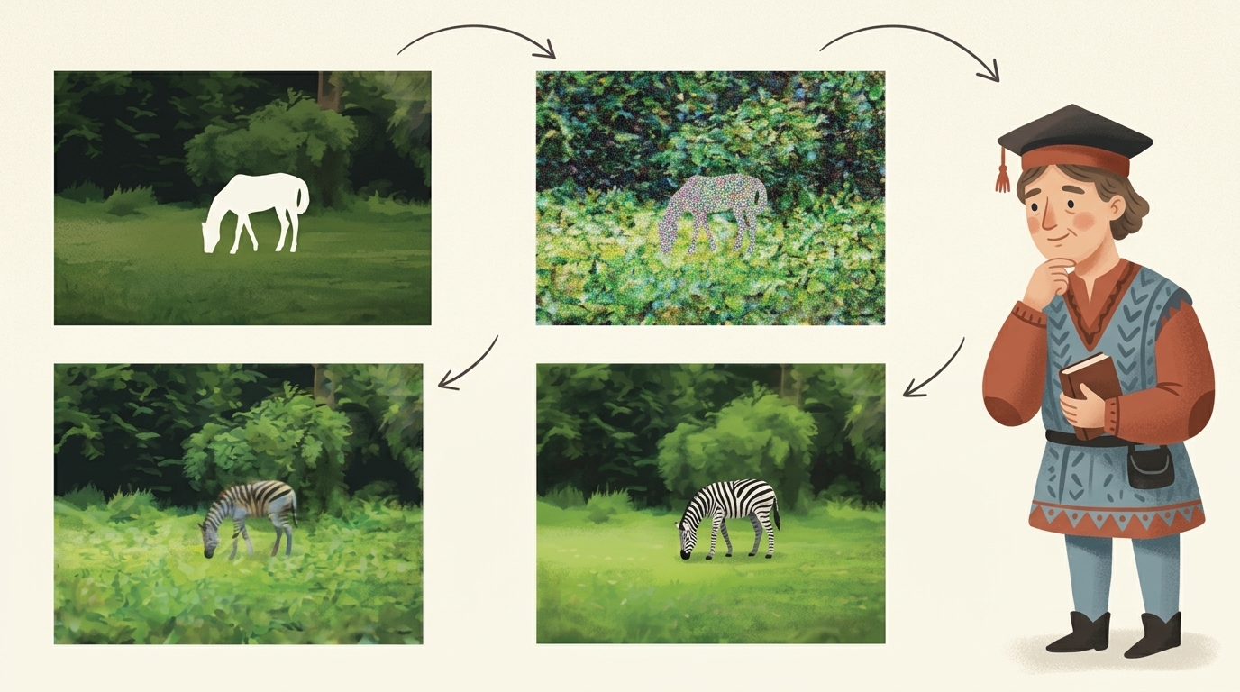
Step 1: Loading the Inpainting Pipeline via Diffusers
We instantiate the Stable Diffusion 2.0 Inpainting pipeline using the open community weights (sd2-community/stable-diffusion-2-inpainting):
from diffusers import StableDiffusionInpaintPipeline
import torch
# Select device and float16 precision for memory efficiency
device = "cuda" if torch.cuda.is_available() else "cpu"
dtype = torch.float16 if device == "cuda" else torch.float32
# Load Stable Diffusion 2.0 Inpainting pipeline
pipe = StableDiffusionInpaintPipeline.from_pretrained(
"sd2-community/stable-diffusion-2-inpainting",
dtype=dtype
).to(device)
# Upcast VAE to Float32 to eliminate FP16 numerical overflow (NaN / Black images)
if device == "cuda" and dtype == torch.float16:
if hasattr(pipe, "upcast_vae"):
pipe.upcast_vae()
else:
pipe.vae.to(dtype=torch.float32)
print(f"Pipeline successfully loaded on device: {device}")
Step 2: Loading Benchmark Image, Binary Mask, and Text Prompt
Inpainting requires three inputs:
image: The original base image ($512 \times 512$).mask_image: A grayscale mask image where white pixels ($255$) indicate the region to be repainted, and black pixels ($0$) remain preserved.prompt: A descriptive text string guiding the diffusion generation.
We load the canonical benchmark image and mask from the official CompVis Latent Diffusion repository:
from PIL import Image
import urllib.request
# Load official Latent Diffusion inpainting benchmark image and mask
img_url = "https://raw.githubusercontent.com/CompVis/latent-diffusion/main/data/inpainting_examples/overture-creations-5sI6fQgYIuo.png"
mask_url = "https://raw.githubusercontent.com/CompVis/latent-diffusion/main/data/inpainting_examples/overture-creations-5sI6fQgYIuo_mask.png"
with urllib.request.urlopen(img_url) as response:
init_image = Image.open(response).convert("RGB").resize((512, 512))
with urllib.request.urlopen(mask_url) as response:
mask_image = Image.open(response).convert("L").resize((512, 512))
prompt = "a sitting cat on a park bench, 8k resolution, photorealistic"
print(f"Base Image Size: {init_image.size} | Mask Image Size: {mask_image.size}")
print(f"Target Text Prompt: '{prompt}'")
Step 3: Executing the Inpainting Denoising Loop
We run diffusion inference with classifier-free guidance scale $7.5$ across $25$ denoising timesteps:
# Execute diffusion sampling loop
with torch.inference_mode():
output = pipe(
prompt=prompt,
image=init_image,
mask_image=mask_image,
num_inference_steps=25,
guidance_scale=7.5,
generator=torch.Generator(device=device).manual_seed(42) if device == "cuda" else None
)
inpainted_image = output.images[0]
print(f"Inpainting complete! Output dimensions: {inpainted_image.size}")
3.2 Unpaired Image-to-Image Translation: CycleGAN (Horse $\to$ Zebra)
In classical supervised learning, image translation requires paired examples $(x_i, y_i)$—such as exact photos of a horse and the exact same scene with a zebra in identical pose and lighting. Because such datasets are virtually impossible to capture, CycleGAN (Zhu et al., 2017) introduced unpaired image-to-image translation.
flowchart LR
X["Domain X (Horse)"] --> G["Generator G\n(X -> Y)"]
G --> FAKE_Y["Generated Zebra G(x)"]
FAKE_Y --> F["Generator F\n(Y -> X)"]
F --> REC_X["Reconstructed Horse F(G(x))"]
REC_X -. "Cycle Consistency: ||F(G(x)) - x||" .-> X
style X fill:#1a1a2e,stroke:#e94560,color:#fff
style G fill:#16213e,stroke:#4cc9f0,color:#fff
style FAKE_Y fill:#0f3460,stroke:#e94560,color:#fff
style F fill:#1b262c,stroke:#00b4d8,color:#fff
style REC_X fill:#2b2d42,stroke:#52b788,color:#fff
The Cycle Consistency Principle
If you translate a sentence from English to French ($G$) and then translate it back from French to English ($F$), you should recover the original sentence. Similarly, in CycleGAN:
$$ F(G(x)) \approx x \quad \text{and} \quad G(F(y)) \approx y $$
The training objective couples adversarial losses ($\mathcal{L}_{\text{GAN}}$) with the $L_1$ Cycle Consistency Loss ($\mathcal{L}_{\text{cyc}}$):
$$ \mathcal{L}_{\text{total}}(G, F, D_X, D_Y) = \mathcal{L}_{\text{GAN}}(G, D_Y, X, Y) + \mathcal{L}_{\text{GAN}}(F, D_X, Y, X) + \lambda \mathcal{L}_{\text{cyc}}(G, F) $$
$$ \mathcal{L}_{\text{cyc}}(G, F) = \mathbb{E}_x \left[ \| F(G(x)) - x \|_1 \right] + \mathbb{E}_y \left[ \| G(F(y)) - y \|_1 \right] $$
Step 1: Instantiating the ResNet Generator
The generator architecture consists of downsampling convolutional blocks, 9 residual blocks (preserving spatial context), and upsampling transpose convolutions:
import torch
import torch.nn as nn
# Define a standard CycleGAN ResNet block
class ResNetBlock(nn.Module):
def __init__(self, dim):
super().__init__()
self.conv_block = nn.Sequential(
nn.ReflectionPad2d(1),
nn.Conv2d(dim, dim, kernel_size=3, padding=0, bias=False),
nn.InstanceNorm2d(dim),
nn.ReLU(True),
nn.ReflectionPad2d(1),
nn.Conv2d(dim, dim, kernel_size=3, padding=0, bias=False),
nn.InstanceNorm2d(dim)
)
def forward(self, x):
return x + self.conv_block(x) # Skip connection
# Instantiate generator skeleton
print("ResNetBlock architecture initialized successfully.")
4. The Hugging Face Ecosystem & Model Zoo
While Torchvision specializes in canonical computer vision architectures, the Hugging Face Hub acts as the universal open-source repository for over 500,000 deep learning models spanning NLP, Vision, Audio, Reinforcement Learning, and Multimodal domains.
flowchart TD
HF["Hugging Face Hub\n(Remote Checkpoint & Config)"] --> CACHE["Local Cache Directory\n(~/.cache/huggingface/hub/)"]
CACHE --> PROC["AutoProcessor / AutoTokenizer\n(Converts Raw Data -> Tensors)"]
CACHE --> MD["AutoModel Class\n(Loads Architecture & Safetensors)"]
PROC & MD --> INF["Inference / Downstream Fine-Tuning"]
style HF fill:#1a1a2e,stroke:#e94560,color:#fff
style CACHE fill:#16213e,stroke:#4cc9f0,color:#fff
style PROC fill:#0f3460,stroke:#00b4d8,color:#fff
style MD fill:#1b262c,stroke:#52b788,color:#fff
style INF fill:#2b2d42,stroke:#fca311,color:#fff
Every Hugging Face model follows two standard components:
- AutoProcessor / AutoTokenizer: Reconstructs the exact tokenization, scaling, vocabulary mapping, and normalization rules used during pretraining.
- AutoModelFor…: Instantiates the neural architecture, downloads weights from remote sharded
.safetensorsfiles, and allocates parameters in memory.
5. Vision-Language Multimodal Inference: BLIP
Vision-Language Models (VLMs) bridge visual perception and natural language generation. BLIP (Bootstrapping Language-Image Pre-training) by Salesforce can perform:
- Unconditional Captioning: Generating rich natural language descriptions of images from scratch.
- Conditional Captioning / VQA: Answering queries about an image or completing text prefix prompts.
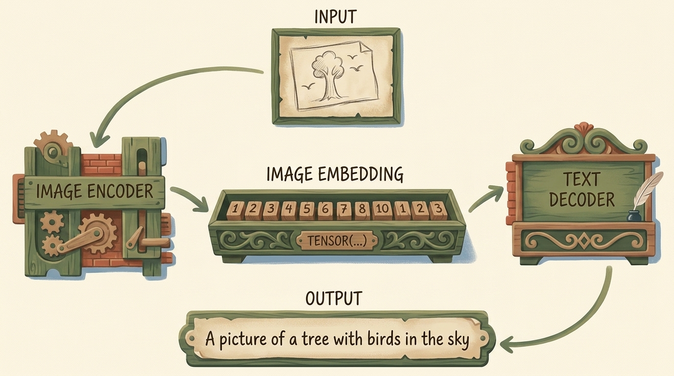
Visual-Text Cross-Attention Mechanism
In the multimodal decoder layers, visual representations are injected into the text generation sequence via Cross-Attention:
$$ \text{CrossAttention}(\mathbf{Q}, \mathbf{K}, \mathbf{V}) = \text{softmax}\left( \frac{\mathbf{Q} \mathbf{K}^T}{\sqrt{d_k}} \right) \mathbf{V} $$
Where queries $\mathbf{Q}$ originate from previous text tokens, and keys $\mathbf{K}$ and values $\mathbf{V}$ originate from the ViT visual token embeddings.
5.1 Executable BLIP Implementation
Step 1: Loading Processor and Model from Hugging Face
We instantiate BlipProcessor and BlipForConditionalGeneration from Salesforce’s base checkpoint:
from transformers import BlipProcessor, BlipForConditionalGeneration
from PIL import Image
import torch
import urllib.request
device = torch.device("cuda" if torch.cuda.is_available() else "cpu")
# 1. Load processor and model
processor = BlipProcessor.from_pretrained("Salesforce/blip-image-captioning-base")
blip_model = BlipForConditionalGeneration.from_pretrained("Salesforce/blip-image-captioning-base").to(device)
blip_model.eval()
print("BLIP model successfully loaded.")
Step 2: Unconditional Image Captioning
We pass a real photo (such as our Golden Retriever) without any guiding prompt to let the model describe the scene from scratch:
# Load sample photo
img_url = "https://raw.githubusercontent.com/pytorch/hub/master/images/dog.jpg"
with urllib.request.urlopen(img_url) as response:
raw_image = Image.open(response).convert("RGB")
# Preprocess image into PyTorch tensors
inputs_unconditional = processor(images=raw_image, return_tensors="pt").to(device)
# Generate caption autoregressively
with torch.inference_mode():
output_tokens = blip_model.generate(**inputs_unconditional, max_new_tokens=30)
caption = processor.decode(output_tokens[0], skip_special_tokens=True)
print(f"Unconditional Caption: '{caption}'")
Step 3: Conditional / Prompt-Guided Captioning
We provide a prefix text prompt (e.g., "a photography of") to steer caption generation:
prompt_text = "a photography of"
# Preprocess both image and conditioning text prompt
inputs_conditional = processor(images=raw_image, text=prompt_text, return_tensors="pt").to(device)
# Generate conditional description
with torch.inference_mode():
output_tokens = blip_model.generate(**inputs_conditional, max_new_tokens=30)
conditional_caption = processor.decode(output_tokens[0], skip_special_tokens=True)
print(f"Conditional Caption: '{conditional_caption}'")
6. Model Sizing, Computational Complexity (FLOPs) & GPU VRAM
When selecting foundation backbones for production deployment, engineers must analyze the trade-off between model accuracy, parameter count, and hardware memory footprint.
6.1 Architectural Comparison Table
| Architecture | Paradigm | Parameter Count | Computational Cost (FLOPs) | ImageNet Top-1 Acc | Primary Use Case |
|---|---|---|---|---|---|
| AlexNet (2012) | Classic CNN | 61.1 M | 0.72 GFLOPs | 56.5% | Historical baseline, education |
| ResNet-18 (2015) | Residual CNN | 11.7 M | 1.82 GFLOPs | 69.8% | Edge devices, IoT, mobile |
| ResNet-101 (2015) | Deep Residual CNN | 44.5 M | 7.85 GFLOPs | 81.9% | Robust spatial visual backbone |
| ViT-B/16 (2020) | Vision Transformer | 86.6 M | 17.60 GFLOPs | 84.2% | High-accuracy foundation vision |
| BLIP-Base (2022) | Multimodal VLM | 223.0 M | ~35.00 GFLOPs | N/A (VQA/Caption) | Image captioning, visual search |
| SD-2.1 Inpaint (2022) | Latent Diffusion | 865.0 M | ~150.00 GFLOPs | N/A (Generative) | Generative image editing |
6.2 Mathematical GPU VRAM Footprint Formula
The static GPU VRAM required to hold model parameters in memory is given by:
$$ \text{VRAM} = N_{\text{params}} \times B_{\text{dtype}} $$
Where $B_{\text{dtype}}$ represents the byte width per parameter:
- FP32 (Single Precision): $B = 4\text{ bytes}$
- FP16 / BF16 (Half Precision): $B = 2\text{ bytes}$
- INT8 (Quantized): $B = 1\text{ byte}$
- INT4 (4-bit NF4 / GPTQ): $B = 0.5\text{ bytes}$
For example, loading ResNet-101 ($44.5 \times 10^6$ parameters) in FP32 requires:
$$ 44.5 \times 10^6 \times 4 \text{ bytes} \approx 178 \text{ MB} $$
Whereas loading Stable Diffusion 2.1 (~$865 \times 10^6$ parameters) in FP16 requires:
$$ 865 \times 10^6 \times 2 \text{ bytes} \approx 1.73 \text{ GB} $$
7. Summary and Key Takeaways
- Transfer Learning Efficiency: Pretrained foundation models eliminate the need to train visual feature extractors from scratch, transferring representations learned on web-scale datasets to specialized downstream tasks.
- Preprocessing Consistency: Input data must strictly match the normalization distribution of the training data (ImageNet channel means $[0.485, 0.456, 0.406]$ and stds $[0.229, 0.224, 0.225]$).
- Execution State Discipline: Always call
model.eval()to freeze stochastic layers (Dropout, BatchNorm) and wrap inference insidewith torch.inference_mode():to eliminate gradient tracking memory overhead. - Multimodal Expansion: Hugging Face and Diffusers provide unified pipelines for multimodal VLMs (BLIP) and generative diffusion models (Stable Diffusion).
It Starts with a Tensor: Storage, Strides, and Memory Layouts
- 1. The World as Floating-Point Numbers
- 2. Tensors: Multidimensional Arrays
- 3. Indexing and Slicing Tensors
- 4. Broadcasting Mechanics
- 5. Named Tensors and Modern Dimension Manipulation (
einops) - 6. Tensor Element Types (
dtype) - 7. The Tensor API & Operation Semantics
- 8. Tensors: Scenic Views of Storage
- 9. Tensor Metadata: Size, Storage Offset, and Strides
- 10. Low-Level Memory Manipulation with
as_strided - 11. Moving Tensors to the GPU
- 12. NumPy Interoperability
- 13. Generalized Tensors
- 14. Serializing Tensors (Checkpoints & HDF5)
- 15. Chapter Exercises & Analytical Solutions
- 16. Summary & Key Architectural Takeaways
Deep neural networks do not operate directly on raw JPEG files, English sentences, or audio waveforms. Before any neural computation, loss evaluation, or backpropagation can take place, input modalities must be translated into multidimensional arrays of numerical floating-point values: tensors.
A tensor is the fundamental mathematical abstraction and primary data structure in PyTorch. However, treating a tensor merely as a nested list or a black-box container overlooks the computational and memory engine that powers modern deep learning. Behind every PyTorch tensor lies a physical, contiguous one-dimensional memory buffer (Storage), indexed via mathematical strides and offsets to enable zero-copy views, high-throughput memory transfers, and GPU acceleration.
This chapter explores the complete anatomy of PyTorch tensors from first principles, following Chapter 3 of Deep Learning with PyTorch (2nd Edition):
- The World as Floating-Point Numbers: How continuous representations enable gradient-based optimization.
- Tensors vs. Python Lists: Boxed object overhead and cache locality vs. contiguous C-level memory allocations.
- Indexing, Slicing & Broadcasting: Multi-axis access patterns and virtual dimension expansion.
- Named Tensors: Semantic dimension tagging and compile-time shape verification.
- Tensor Data Types (
dtype): Numeric precision formats (float32,bfloat16,float16,int64) and memory consumption. - The Tensor API & In-Place Semantics: Functional transformations, dimension reductions, and the mutation safety rules of trailing underscores (
_). - Physical Storage Anatomy: The 1D contiguous
Storagebuffer, raw memory pointers, and untyped allocations. - Stride Mathematics & Zero-Copy Views: The offset mapping formula $\text{Offset} = \text{storage\_offset} + \sum_{k=0}^{n-1} i_k \cdot \text{stride}[k]$, dimension transpositions (
.t(),.permute()), and memory contiguity (.is_contiguous(),.contiguous()). - Low-Level Memory Manipulation: Surgical strided windows via
as_strided(). - Hardware Device Management: Host RAM $\leftrightarrow$ GPU VRAM transfers, CUDA streams, and pinned memory buffers.
- NumPy Interoperability: Zero-copy buffer sharing between Python scientific ecosystems.
- Generalized Tensors: Quantized, sparse, and nested tensor abstractions.
- Serialization & Persistence: PyTorch checkpoints (
torch.save/torch.load) and high-performance HDF5 (h5py) storage. - Chapter Exercises & Analytical Solutions: Rigorous breakdown of Chapter 3’s memory and storage problems.
1. The World as Floating-Point Numbers
In traditional symbolic artificial intelligence, knowledge was encoded through discrete symbols (such as truth tables, graph nodes, and Boolean predicates). Deep learning fundamentally replaces discrete symbol manipulation with geometric transformations over continuous vector spaces.
flowchart TD
subgraph Inputs["1. Real-World Inputs"]
I1["High-Resolution Images"]
I2["Audio Waveforms"]
I3["Natural Language Tokens"]
I4["Clinical Medical Records"]
end
subgraph Encoding["2. Continuous Tensor Encoding"]
E["Multidimensional Floating-Point Grid\n(float32 / bfloat16 Tensors)"]
end
subgraph Manifold["3. Latent Manifold & Differentiable Operations"]
M["Geometric Warping & Linear / Non-Linear Layers\n(Analytical Gradients via Calculus)"]
end
subgraph Target["4. Interpretable Predictions"]
O["Class Probabilities / Bounding Boxes / Synthesized Audio"]
end
Inputs --> Encoding --> Manifold --> Target
style Inputs fill:#1a1a2e,stroke:#e94560,color:#fff
style Encoding fill:#16213e,stroke:#4cc9f0,color:#fff
style Manifold fill:#0f3460,stroke:#00b4d8,color:#fff
style Target fill:#1b262c,stroke:#52b788,color:#fff
Floating-point numbers allow neural networks to compute infinitesimally small directional updates via calculus. When an image pixel changes slightly in intensity, the corresponding model loss changes continuously:
$$ \lim_{\Delta x \to 0} \frac{f(x + \Delta x) - f(x)}{\Delta x} = \frac{\partial f}{\partial x} $$
Because floating-point numbers approximate real numbers ($\mathbb{R}$), gradient descent can smoothly steer millions of model weights toward low-loss configurations on a high-dimensional loss surface.
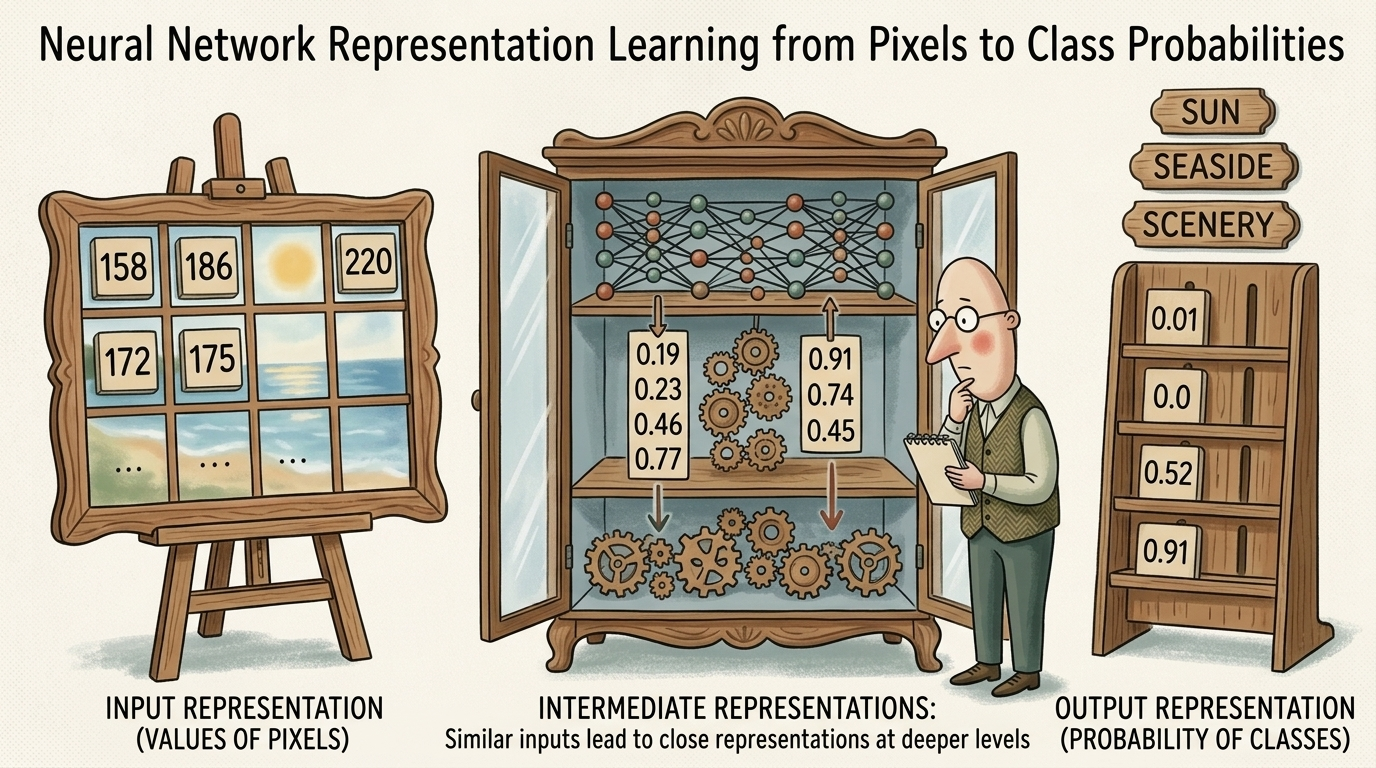
Key Insight: Deep learning models are continuous function approximators. Tensors of floating-point numbers provide the substrate upon which differentiable optimization operates.
2. Tensors: Multidimensional Arrays
At a mathematical level, a scalar is a 0D tensor, a vector is a 1D tensor, a matrix is a 2D tensor, and an array with three or more axes is an N-dimensional tensor.
flowchart TD
subgraph DimensionHierarchy["Tensor Dimensionality Hierarchy"]
D0["0D Tensor (Scalar)\nShape: [] | Example: Loss value = 0.425"]
D1["1D Tensor (Vector)\nShape: [3] | Example: Audio amplitude sequence"]
D2["2D Tensor (Matrix)\nShape: [4, 3] | Example: Linear layer weights"]
D3["3D Tensor\nShape: [3, 256, 256] | Example: RGB Image (C x H x W)"]
D4["4D Tensor\nShape: [32, 3, 224, 224] | Example: Batch of Images (B x C x H x W)"]
D5["5D Tensor\nShape: [8, 1, 64, 128, 128] | Example: Batch of 3D CT Scans (B x C x D x H x W)"]
end
D0 --> D1 --> D2 --> D3 --> D4 --> D5
style D0 fill:#1a1a2e,stroke:#e94560,color:#fff
style D1 fill:#16213e,stroke:#4cc9f0,color:#fff
style D2 fill:#0f3460,stroke:#00b4d8,color:#fff
style D3 fill:#1b262c,stroke:#52b788,color:#fff
style D4 fill:#2b2d42,stroke:#e94560,color:#fff
style D5 fill:#3a0ca3,stroke:#4cc9f0,color:#fff
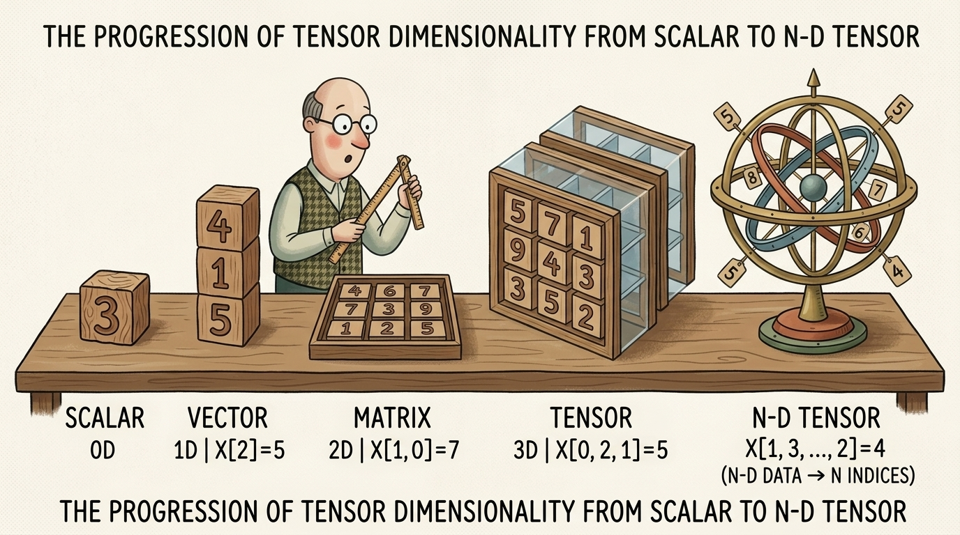
2.1 From Python Lists to PyTorch Tensors
Why not simply use native Python lists (list) of numbers? Python is an interpreted, dynamically typed language. In a native Python list:
- Every number is wrapped in a full
PyObjectstructure on the heap (boxed representation), consuming up to 24–28 bytes for a single 64-bit integer or float. - The list itself is an array of memory pointers pointing to scattered heap locations. Accessing elements requires pointer dereferencing, causing massive CPU cache misses.
- Python lists cannot be executed on SIMD vector registers or dispatched to GPU compute cores.
flowchart TD
subgraph PythonList["1. Python List (Scattered Heap Objects)"]
direction TB
L["Python List: [ Ptr 0 | Ptr 1 | Ptr 2 | Ptr 3 ]"]
P0["• Ptr 0 -> PyObject(1.0) on Heap (24B)"]
P1["• Ptr 1 -> PyObject(2.0) on Heap (24B)"]
P2["• Ptr 2 -> PyObject(3.0) on Heap (24B)"]
P3["• Ptr 3 -> PyObject(4.0) on Heap (24B)"]
L --> P0 --> P1 --> P2 --> P3
end
subgraph PyTorchTensor["2. PyTorch Tensor (Contiguous C Memory)"]
direction TB
T["Tensor Object (Metadata):<br/>Shape: (4,) | Stride: (1,) | Offset: 0"]
S["Contiguous 1D C-Array in RAM/VRAM:<br/>[ 1.0f | 2.0f | 3.0f | 4.0f ]<br/>Total: Exactly 16 Bytes (SIMD / GPU Vectorized)"]
T --> S
end
PythonList -->|Architectural Paradigm Shift| PyTorchTensor
style PythonList fill:#1a1a2e,stroke:#e94560,color:#fff
style PyTorchTensor fill:#16213e,stroke:#4cc9f0,color:#fff
style S fill:#0f3460,stroke:#52b788,color:#fff
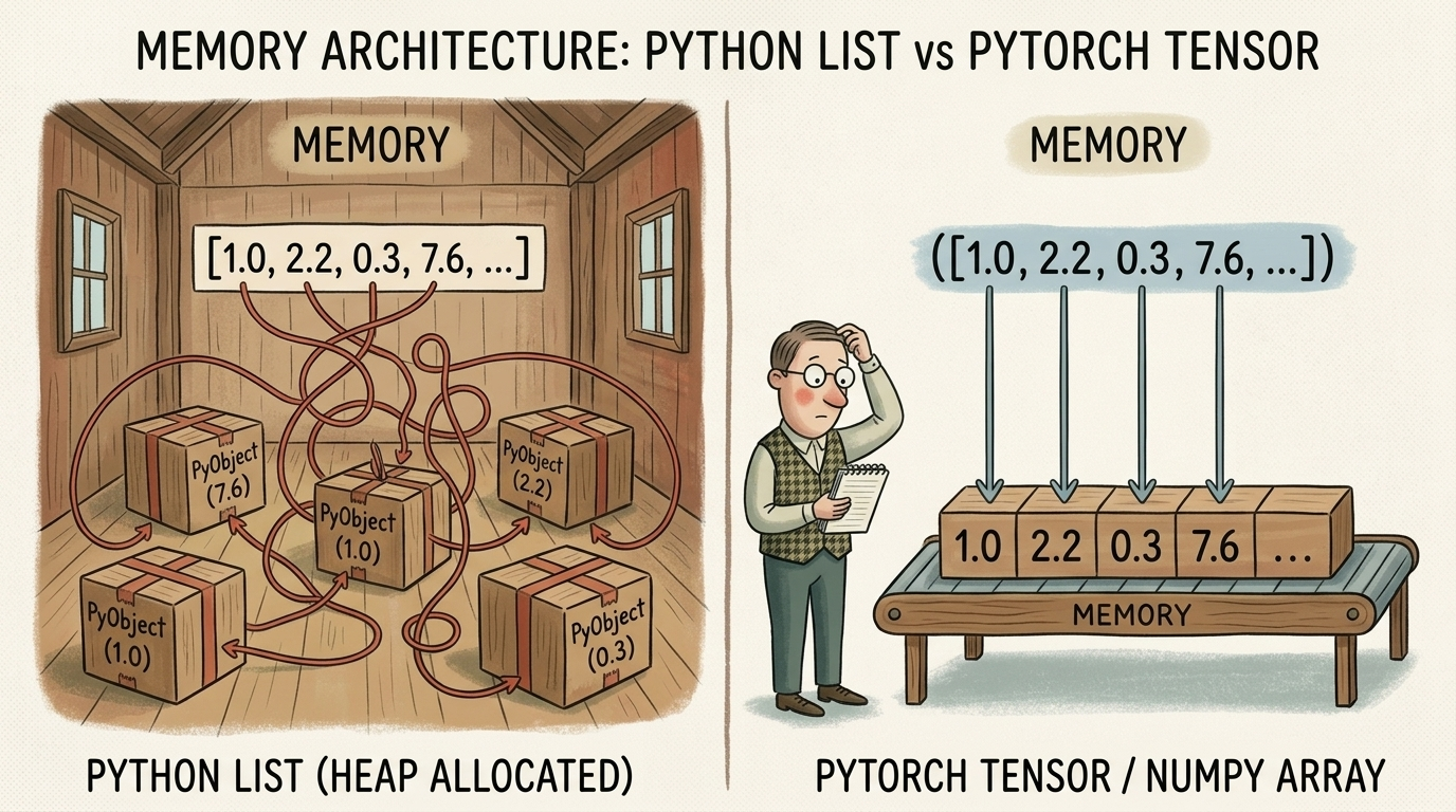
In contrast, a PyTorch torch.Tensor stores raw, unboxed binary values directly in a contiguous block of memory allocated in C/C++ memory. A 1,000,000-element float32 tensor occupies exactly $1{,}000{,}000 \times 4 \text{ bytes} = 4 \text{ MB}$, loaded cleanly into CPU L1/L2/L3 caches and vectorized via AVX-512 or CUDA cores.
2.2 Constructing Our First Tensors
Let us initialize our first PyTorch tensors using primary creation factory functions. We specify dimensions and verify their shapes, element counts, and dimensions.
First, import PyTorch and construct a 1D tensor from a native Python list:
import torch
# Construct a 1D tensor from a Python list
a = torch.tensor([1.0, 2.0, 3.0])
print(f"Tensor a: {a}")
print(f"Shape: {a.shape} | Number of elements: {a.numel()} | Dimension rank: {a.dim()}")
Next, create multidimensional tensors populated with constant values (ones, zeros, or uniform random values) without allocating intermediate Python lists:
# Create a 2D tensor of ones with 3 rows and 2 columns
ones_2d = torch.ones(3, 2)
print(f"2D Ones Tensor (3x2):\n{ones_2d}")
# Create a 3D tensor of zeros representing 2 channels of 4x4 spatial grids
zeros_3d = torch.zeros(2, 4, 4)
print(f"3D Zeros Tensor (2x4x4) shape: {zeros_3d.shape}")
3. Indexing and Slicing Tensors
PyTorch tensors support the complete Python slicing syntax, identical to NumPy arrays. Slicing along multiple dimensions allows sub-region extraction, row/column slicing, and negative indexing.
flowchart TD
subgraph Matrix2D["2D Tensor: Shape [3, 4]"]
R0["Row 0: [ 10, 11, 12, 13 ]"]
R1["Row 1: [ 20, 21, 22, 23 ]"]
R2["Row 2: [ 30, 31, 32, 33 ]"]
end
subgraph SliceExtraction["Sub-Tensor Slice: tensor[1:, 1:3]"]
S0["Row 1, Cols 1..2: [ 21, 22 ]"]
S1["Row 2, Cols 1..2: [ 31, 32 ]"]
end
Matrix2D -->|Zero-Copy Slicing| SliceExtraction
style Matrix2D fill:#1a1a2e,stroke:#e94560,color:#fff
style SliceExtraction fill:#16213e,stroke:#4cc9f0,color:#fff
Let us construct a $3 \times 4$ matrix and extract sub-tensors using multidimensional slicing:
# Construct a 3x4 tensor with sequential values from 1 to 12
grid = torch.arange(1, 13, dtype=torch.float32).reshape(3, 4)
print(f"Original 3x4 grid:\n{grid}")
# Extract a single scalar element at row index 1, column index 2
element = grid[1, 2]
print(f"Element at row 1, col 2: {element.item()}")
# Extract all rows for column 0 (1D slice)
first_column = grid[:, 0]
print(f"First column (all rows, col 0): {first_column}")
# Extract a 2x2 sub-matrix: rows 1 to end, columns 1 to 3 (exclusive)
sub_grid = grid[1:, 1:3]
print(f"Sub-matrix grid[1:, 1:3]:\n{sub_grid}")
4. Broadcasting Mechanics
When performing element-wise arithmetic operations between two tensors of differing dimensions, PyTorch automatically applies broadcasting rules (inherited from NumPy). Broadcasting virtually expands singleton dimensions (dimensions of size 1) without physically duplicating memory in RAM or VRAM.
flowchart TD
subgraph Inputs["1. Operands with Mismatched Shapes"]
direction TB
A["Tensor A: Shape (3, 1)<br/>Column Vector: [ [10], [20], [30] ]"]
B["Tensor B: Shape (1, 4)<br/>Row Vector: [ [1, 2, 3, 4] ]"]
A --> B
end
subgraph Expansion["2. Zero-Copy Virtual Expansion"]
direction TB
EXP["Broadcasting Alignment Rules:<br/>• Dim 1 of A expands: (3, 1) -> (3, 4)<br/>• Dim 0 of B expands: (1, 4) -> (3, 4)<br/>(Virtual stride=0 expansion without RAM allocation)"]
end
subgraph Result["3. Broadcasted Addition Output"]
direction TB
OUT["Result A + B: Shape (3, 4)<br/>Row 0: [ 11, 12, 13, 14 ]<br/>Row 1: [ 21, 22, 23, 24 ]<br/>Row 2: [ 31, 32, 33, 34 ]"]
end
Inputs --> Expansion --> Result
style Inputs fill:#1a1a2e,stroke:#e94560,color:#fff
style Expansion fill:#16213e,stroke:#4cc9f0,color:#fff
style Result fill:#0f3460,stroke:#52b788,color:#fff
The Two Rules of Broadcasting:
- Dimension Alignment: Alignment begins from the trailing (rightmost) dimension and works backwards to the leading dimension.
- Compatibility Condition: Two dimensions are compatible if:
- They are equal in size, or
- One of them is equal to $1$, or
- One of the dimensions does not exist (prepended virtually with size $1$).
Let us demonstrate broadcasting in practice:
# Construct a (3, 1) column vector
col_vector = torch.tensor([[10.0], [20.0], [30.0]])
print(f"col_vector shape: {col_vector.shape}")
# Construct a (1, 4) row vector
row_vector = torch.tensor([[1.0, 2.0, 3.0, 4.0]])
print(f"row_vector shape: {row_vector.shape}")
# Broadcasted addition produces a (3, 4) matrix with zero data replication
broadcasted_sum = col_vector + row_vector
print(f"Broadcasted result shape: {broadcasted_sum.shape}")
print(f"Broadcasted result values:\n{broadcasted_sum}")
5. Named Tensors and Modern Dimension Manipulation (einops)
In production deep learning pipelines with 4D or 5D tensors (e.g. [Batch, Channel, Height, Width] in Computer Vision or [Batch, Sequence, Heads, HeadDim] in Transformers), indexing by positional integers (such as x.transpose(1, 2)) frequently causes subtle transposition bugs.
PyTorch introduced Named Tensors as an experimental feature allowing dimensions to be tagged with explicit string identifiers:
# Create a 4D tensor with explicit dimension names (Experimental PyTorch API)
images = torch.zeros(2, 3, 28, 28, names=('batch', 'channels', 'rows', 'cols'))
print(f"Named Tensor dimensions: {images.names}")
# Reorder dimensions using align_to without memorizing integer axis indices
reordered_images = images.align_to('batch', 'rows', 'cols', 'channels')
print(f"Reordered tensor dimensions: {reordered_images.names}")
print(f"Reordered tensor shape: {reordered_images.shape}")
5.1 The Modern Industry Standard: einops
While native Named Tensors provided a compelling concept, they remained experimental with limited PyTorch operator support. In modern deep learning (PyTorch 2.x+) and production Vision Transformer / LLM codebases, the undisputed industry standard for dimension manipulation is einops (from einops import rearrange, reduce, repeat).
einops provides expressive, declarative, and self-documenting tensor transformations across PyTorch, JAX, and TensorFlow:
flowchart TD
subgraph Positional["1. Positional Permutations (Error-Prone)"]
direction TB
P["img.permute(0, 2, 3, 1)<br/>• Silent bugs if tensor is NCHW vs NHWC<br/>• Unreadable in multi-head attention"]
end
subgraph NamedNative["2. PyTorch Named Tensors (Experimental)"]
direction TB
N["img.align_to('batch', 'rows', 'cols', 'channels')<br/>• Explicit dimension tags<br/>• Limited operator support in PyTorch 2.x"]
end
subgraph EinopsModern["3. Modern Industry Standard: einops (Production)"]
direction TB
E["rearrange(imgs, 'b c h w -> b h w c')<br/>• Declarative & self-documenting syntax<br/>• Standard in ViTs, Diffusion Models & LLMs"]
end
Positional --> NamedNative --> EinopsModern
style Positional fill:#1a1a2e,stroke:#e94560,color:#fff
style NamedNative fill:#16213e,stroke:#4cc9f0,color:#fff
style EinopsModern fill:#0f3460,stroke:#52b788,color:#fff
Let us demonstrate dimension rearrangement using einops:
# %pip install einops
import torch
from einops import rearrange
# 1. Construct input tensor in NCHW format
imgs = torch.randn(2, 3, 28, 28)
# 2. Declare dimension names and transform to target layout (NCHW -> NHWC)
imgs_reordered = rearrange(imgs, 'batch channels rows cols -> batch rows cols channels')
print("Original Shape :", imgs.shape) # torch.Size([2, 3, 28, 28])
print("Reordered Shape:", imgs_reordered.shape) # torch.Size([2, 28, 28, 3])
6. Tensor Element Types (dtype)
A tensor’s numeric representation is determined by its dtype (data type). Choosing the appropriate precision format is crucial for balancing mathematical precision, memory consumption, and GPU arithmetic throughput.
flowchart TD
subgraph FloatingTypes["1. Floating-Point Formats"]
direction TB
F64["torch.float64 (Double)<br/>• 64 bits (8 bytes)<br/>• High-precision physics & PDE solving"]
F32["torch.float32 (Float)<br/>• 32 bits (4 bytes)<br/>• Standard deep learning training default"]
BF16["torch.bfloat16 (Brain Float)<br/>• 16 bits (2 bytes)<br/>• 8-bit dynamic range + 7-bit precision<br/>• Standard for Modern LLMs & Ampere/Hopper"]
F16["torch.float16 (Half)<br/>• 16 bits (2 bytes)<br/>• Legacy mixed precision"]
F64 --> F32 --> BF16 --> F16
end
subgraph IntegerTypes["2. Integer & Boolean Types"]
direction TB
I64["torch.int64 (Long)<br/>• 64 bits (8 bytes)<br/>• Target classification labels & token IDs"]
I32["torch.int32 (Int)<br/>• 32 bits (4 bytes)<br/>• Standard C integer indexing"]
U8["torch.uint8 (Byte)<br/>• 8 bits (1 byte)<br/>• Raw pixel values (0-255)"]
B1["torch.bool (Bool)<br/>• 8 bits (1 byte)<br/>• Binary masks & boolean logic"]
I64 --> I32 --> U8 --> B1
end
FloatingTypes --> IntegerTypes
style FloatingTypes fill:#1a1a2e,stroke:#e94560,color:#fff
style IntegerTypes fill:#16213e,stroke:#4cc9f0,color:#fff
style F32 fill:#0f3460,stroke:#4cc9f0,color:#fff
style BF16 fill:#1b262c,stroke:#52b788,color:#fff
6.1 Precision Comparison Table
| Data Type | PyTorch Type Name | Size in Bytes | Dynamic Range (Exponent) | Numerical Precision (Mantissa) | Typical Application |
|---|---|---|---|---|---|
| Double | torch.float64 / torch.double | 8 bytes (64 bits) | 11 bits | 52 bits | High-precision physics & PDE solving |
| Float | torch.float32 / torch.float | 4 bytes (32 bits) | 8 bits | 23 bits | Standard training default |
| Bfloat16 | torch.bfloat16 | 2 bytes (16 bits) | 8 bits (same as fp32) | 7 bits | Modern LLM / Transformer mixed precision |
| Half | torch.float16 / torch.half | 2 bytes (16 bits) | 5 bits | 10 bits | Legacy GPU mixed precision (requires loss scaling) |
| Long | torch.int64 / torch.long | 8 bytes (64 bits) | N/A | N/A | Target labels, embedding lookup indices |
| Byte | torch.uint8 | 1 byte (8 bits) | N/A | N/A | Raw uint8 image datasets ($0 \dots 255$) |
6.2 Managing and Casting dtype
Let us inspect the default dtype and convert between precision formats using .to() and convenient casting aliases:
# Default float tensor creation uses float32
default_float = torch.tensor([1.0, 2.0, 3.0])
print(f"Default float dtype: {default_float.dtype}")
# Explicitly cast to bfloat16 for high-throughput memory-efficient training
bf16_tensor = default_float.to(dtype=torch.bfloat16)
print(f"Cast to bfloat16: {bf16_tensor.dtype} | Element size: {bf16_tensor.element_size()} bytes")
# Integer casting for target classification labels
int_labels = torch.tensor([0, 2, 1], dtype=torch.int64)
print(f"Classification labels dtype: {int_labels.dtype}")
7. The Tensor API & Operation Semantics
The PyTorch Tensor API provides hundreds of operators spanning mathematical functions, linear algebra routines, and shape reductions.

7.1 Mathematical Functions and Dimensional Reductions
Most mathematical operations (torch.sin, torch.exp, torch.sqrt, etc.) operate element-wise. Reduction operations like torch.mean and torch.sum allow collapsing specific axes using the dim parameter.
flowchart TD
subgraph MatrixInput["Input Tensor: Shape (2, 3)"]
M0["[ [ 1.0, 2.0, 3.0 ],\n [ 4.0, 5.0, 6.0 ] ]"]
end
subgraph Dim0["Reduction along dim=0 (Columns Collapsed)"]
D0["torch.mean(t, dim=0) -> Shape (3,)\n[ 2.5, 3.5, 4.5 ]"]
end
subgraph Dim1["Reduction along dim=1 (Rows Collapsed, keepdim=True)"]
D1["torch.mean(t, dim=1, keepdim=True) -> Shape (2, 1)\n[ [ 2.0 ],\n [ 5.0 ] ]"]
end
MatrixInput --> Dim0
MatrixInput --> Dim1
style MatrixInput fill:#1a1a2e,stroke:#e94560,color:#fff
style Dim0 fill:#16213e,stroke:#4cc9f0,color:#fff
style Dim1 fill:#0f3460,stroke:#52b788,color:#fff
Let us compute dimensional reductions:
# Construct a 2x3 matrix
matrix = torch.tensor([[1.0, 2.0, 3.0], [4.0, 5.0, 6.0]])
# Reduce along dimension 0 (collapse rows -> compute column averages)
mean_dim0 = torch.mean(matrix, dim=0)
print(f"Mean across dim=0: {mean_dim0} | Shape: {mean_dim0.shape}")
# Reduce along dimension 1 with keepdim=True (preserves 2D rank)
mean_dim1_kept = torch.mean(matrix, dim=1, keepdim=True)
print(f"Mean across dim=1 (keepdim=True):\n{mean_dim1_kept} | Shape: {mean_dim1_kept.shape}")
7.2 In-Place Operations (_ Suffix)
Any operation in PyTorch that ends with a trailing underscore (such as .zero_(), .add_(), .mul_(), .copy_()) mutates the tensor’s underlying memory in-place rather than allocating a new tensor.
Warning
Autograd In-Place Safety Rule: In-place operations mutate memory buffers directly. If an in-place modification overwrites a tensor value required later during the backward pass for gradient computation, PyTorch’s Autograd engine will throw a runtime error. Use in-place operations with caution in differentiable computational graphs.
# Create a tensor and mutate its values in-place
x = torch.ones(2, 2)
print(f"Original x:\n{x}")
# Add 5 to every element in-place
x.add_(5.0)
print(f"x after x.add_(5.0):\n{x}")
# In-place zeroing out of the entire tensor
x.zero_()
print(f"x after x.zero_():\n{x}")
8. Tensors: Scenic Views of Storage
To master PyTorch performance, one must understand how memory is physically structured. A torch.Tensor is fundamentally a lightweight view object containing metadata (shape, stride, storage_offset, dtype, device), which references a single contiguous 1D memory array: the Storage buffer.
flowchart TD
subgraph LogicalView["Logical 2D View (Tensor Object)"]
T["Tensor: Shape (3, 2)\nStorage Offset: 0\nStrides: (2, 1)"]
R0["Row 0: [ (0,0)=1.0 , (0,1)=2.0 ]"]
R1["Row 1: [ (1,0)=3.0 , (1,1)=4.0 ]"]
R2["Row 2: [ (2,0)=5.0 , (2,1)=6.0 ]"]
T --- R0 & R1 & R2
end
subgraph PhysicalMemory["Physical 1D Memory (Storage Buffer)"]
S["UntypedStorage (6 consecutive float32 numbers in RAM/VRAM)\n[ 1.0 | 2.0 | 3.0 | 4.0 | 5.0 | 6.0 ]\nByte Offsets: [ 0B | 4B | 8B | 12B | 16B | 20B ]"]
end
LogicalView -->|Indexed via Strides| PhysicalMemory
style LogicalView fill:#1a1a2e,stroke:#e94560,color:#fff
style PhysicalMemory fill:#16213e,stroke:#4cc9f0,color:#fff
style S fill:#0f3460,stroke:#52b788,color:#fff
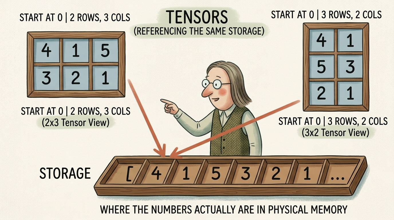
8.1 Inspecting the Underlying 1D Storage (UntypedStorage in PyTorch 2.x)
Let us inspect the storage buffer of a 2D tensor using .untyped_storage():
# Construct a 2D tensor of shape (3, 2)
points = torch.tensor([[1.0, 2.0], [3.0, 4.0], [5.0, 6.0]])
print(f"Tensor points (3x2):
{points}")
# Access the physical 1D storage
points_storage = points.untyped_storage()
print(f"Physical 1D Storage byte size: {len(points_storage)} bytes")
print(f"Storage raw byte contents: {[points_storage[i] for i in range(len(points_storage))]}")
Note
PyTorch 2.x
UntypedStorageArchitecture:
In older PyTorch versions,points.storage()returned a type-aware storage (such asFloatStorage). In modern PyTorch 2.x+,.untyped_storage()manages raw binary bytes (uint8). Consequently,len(points_storage)returns the total number of bytes ($6 \text{ float32 elements} \times 4 \text{ bytes} = 24 \text{ bytes}$), not the logical element count.
8.2 Modifying Storage Mutates All Views
Because multiple tensor views point to the exact same physical storage buffer, mutating values through one view or directly in storage immediately alters all other views sharing that storage.
When indexing UntypedStorage directly, values must be assigned as integer bytes ($0 \dots 255$ int). Alternatively, mutating via any logical tensor view updates the float representation across all sharing views:
# 1. Mutating the underlying storage byte directly (must be an integer byte 0-255 in PyTorch 2.x)
points_storage[0] = 99
# 2. Or mutating via a tensor view (floating-point mutation)
points[0, 0] = 99.0
# The 2D tensor view and all shared views reflect the change immediately
print(f"Points tensor after mutation:
{points}")
9. Tensor Metadata: Size, Storage Offset, and Strides
How does PyTorch translate a multidimensional coordinate $(i_0, i_1, \dots, i_{n-1})$ into a 1D flat storage index? It evaluates the stride linear mapping equation:
$$ \text{Physical Storage Offset} = \text{storage\_offset} + \sum_{k=0}^{n-1} i_k \cdot \text{stride}[k] $$
Where:
- $\text{storage\_offset}$: The index in the 1D storage corresponding to the first element of the tensor $(0, 0, \dots, 0)$.
- $\text{stride}[k]$: The number of physical 1D elements one must skip in memory to advance by 1 unit along dimension $k$.
flowchart TD
subgraph StrideFormula["1. Stride Mapping Formula"]
direction TB
F["Storage Index = Offset + (Row * Stride[0]) + (Col * Stride[1])<br/>For Shape (3, 2), Strides (2, 1), Offset 0:"]
end
subgraph Row0["2. Row 0 Coordinates"]
direction TB
R0["• (0, 0) -> 0*2 + 0*1 = Storage[0] (1.0)<br/>• (0, 1) -> 0*2 + 1*1 = Storage[1] (2.0)"]
end
subgraph Row1["3. Row 1 Coordinates"]
direction TB
R1["• (1, 0) -> 1*2 + 0*1 = Storage[2] (3.0)<br/>• (1, 1) -> 1*2 + 1*1 = Storage[3] (4.0)"]
end
subgraph Row2["4. Row 2 Coordinates"]
direction TB
R2["• (2, 0) -> 2*2 + 0*1 = Storage[4] (5.0)<br/>• (2, 1) -> 2*2 + 1*1 = Storage[5] (6.0)"]
end
StrideFormula --> Row0 --> Row1 --> Row2
style StrideFormula fill:#1a1a2e,stroke:#e94560,color:#fff
style Row0 fill:#16213e,stroke:#4cc9f0,color:#fff
style Row1 fill:#0f3460,stroke:#00b4d8,color:#fff
style Row2 fill:#1b262c,stroke:#52b788,color:#fff
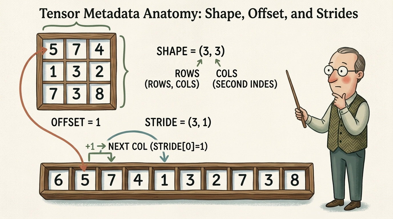
9.1 Slicing Creates Sub-Tensor Views (Zero Memory Allocation)
When we slice a tensor (e.g. second_point = points[1]), PyTorch does not allocate new memory or copy data. It merely creates a new torch.Tensor header pointing to the same storage with an updated storage_offset:
# Construct points tensor
points = torch.tensor([[1.0, 2.0], [3.0, 4.0], [5.0, 6.0]])
# Extract the second row (index 1)
second_point = points[1]
print(f"second_point values: {second_point}")
print(f"second_point shape: {second_point.shape}")
print(f"second_point storage_offset: {second_point.storage_offset()}")
print(f"second_point stride: {second_point.stride()}")
# Verify that points and second_point share the exact same underlying storage pointer
print(f"Shared storage: {points.untyped_storage().data_ptr() == second_point.untyped_storage().data_ptr()}")
9.2 Transposing Without Copying (Zero-Copy Transposition)
To transpose a 2D matrix from shape $(M, N)$ to $(N, M)$, PyTorch does not reorder numbers in RAM. It simply swaps the strides of dimension 0 and dimension 1:
flowchart TD
subgraph OriginalTensor["Original Tensor: Shape (3, 2) | Strides (2, 1)"]
O_desc["Element (r, c) = Storage[r * 2 + c * 1]"]
end
subgraph TransposedTensor["Transposed Tensor: Shape (2, 3) | Strides (1, 2)"]
T_desc["Element (r, c) = Storage[r * 1 + c * 2] (Zero Data Moved)"]
end
subgraph SameStorage["Shared 1D Storage Buffer"]
S["[ 1.0, 2.0, 3.0, 4.0, 5.0, 6.0 ]"]
end
OriginalTensor -->|Zero-Copy Metadata Update| TransposedTensor
OriginalTensor --> SameStorage
TransposedTensor --> SameStorage
style OriginalTensor fill:#1a1a2e,stroke:#e94560,color:#fff
style TransposedTensor fill:#16213e,stroke:#4cc9f0,color:#fff
style SameStorage fill:#0f3460,stroke:#52b788,color:#fff
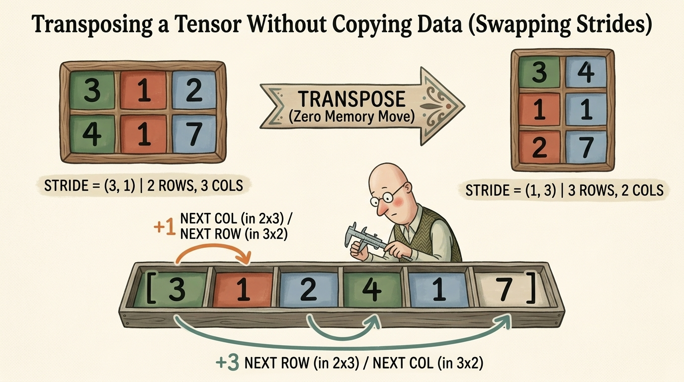
Let us verify transposition strides in Python:
# Original 3x2 tensor
points = torch.tensor([[1.0, 2.0], [3.0, 4.0], [5.0, 6.0]])
print(f"points shape: {points.shape} | stride: {points.stride()}")
# Transpose the 2D tensor
points_t = points.t()
print(f"points_t shape: {points_t.shape} | stride: {points_t.stride()}")
print(f"points_t values:\n{points_t}")
# Verify data pointer identity
print(f"Memory shared: {points.data_ptr() == points_t.data_ptr()}")
9.3 Higher-Dimensional Transposition (.permute() & .transpose())
For tensors with 3 or more dimensions, torch.transpose swaps two specified dimensions, while .permute() reorders all axes simultaneously:
# Create a 3D tensor of shape (2, 3, 4)
tensor_3d = torch.zeros(2, 3, 4)
print(f"tensor_3d shape: {tensor_3d.shape} | stride: {tensor_3d.stride()}")
# Permute dimensions to (4, 2, 3)
permuted_3d = tensor_3d.permute(2, 0, 1)
print(f"permuted_3d shape: {permuted_3d.shape} | stride: {permuted_3d.stride()}")
9.4 Memory Contiguity (.is_contiguous() and .contiguous())
A tensor is defined as C-contiguous (row-major order) if traversing elements in sequential index order visits physical 1D storage elements in strict sequential order $0, 1, 2, \dots$ without jumps.
When a tensor is transposed, its strides are swapped, making the layout non-contiguous. Many high-performance operations (such as .view(), FFTs, and CUDA custom kernels) require contiguous memory layouts.
flowchart TD
subgraph ContiguityFlow["Tensor Memory Contiguity Pipeline"]
C["1. Contiguous Tensor (points)\n- points.is_contiguous() == True\n- Storage order matches row-major traversal"]
N["2. Non-Contiguous Tensor (points_t = points.t())\n- points_t.is_contiguous() == False\n- Strides swapped: (1, 2). Attempting .view() fails!"]
R["3. Calling .contiguous() (points_t.contiguous())\n- Allocates NEW contiguous 1D Storage buffer\n- Re-aligns memory in row-major order so .view() succeeds"]
end
C -->|Transpose swaps strides| N -->|Physical memory reordering| R
style ContiguityFlow fill:#1a1a2e,stroke:#e94560,color:#fff
style C fill:#16213e,stroke:#52b788,color:#fff
style N fill:#0f3460,stroke:#e94560,color:#fff
style R fill:#2b2d42,stroke:#4cc9f0,color:#fff
Let us examine contiguity in code:
# Check contiguity of original and transposed tensors
print(f"points.is_contiguous(): {points.is_contiguous()}")
print(f"points_t.is_contiguous(): {points_t.is_contiguous()}")
# Attempting .view() on a non-contiguous tensor raises a RuntimeError
try:
points_t.view(6)
except RuntimeError as e:
print(f"Expected view error on non-contiguous tensor: {e}")
# .contiguous() copies elements into a fresh, contiguous storage buffer
points_t_cont = points_t.contiguous()
print(f"points_t_cont.is_contiguous(): {points_t_cont.is_contiguous()}")
print(f"points_t_cont stride: {points_t_cont.stride()}")
print(f"points_t_cont.view(6) works: {points_t_cont.view(6)}")
10. Low-Level Memory Manipulation with as_strided
For custom low-level operations (such as convolution sliding windows or image patch extraction), PyTorch allows creating custom tensor views by defining exact size, stride, and storage_offset parameters via torch.as_strided().
# Construct a 1D tensor with sequential values
base = torch.arange(10, dtype=torch.float32)
print(f"Base 1D tensor: {base}")
# Create a 2D sliding window view of shape (7, 4) with stride (1, 1)
# Window size = 4, Step = 1 across 10 elements -> 7 windows
sliding_windows = base.as_strided(size=(7, 4), stride=(1, 1), storage_offset=0)
print(f"Sliding window view (zero copy!):\n{sliding_windows}")
11. Moving Tensors to the GPU
PyTorch allows executing tensor operations on hardware accelerators (NVIDIA CUDA GPUs, Apple MPS, AMD ROCm). A tensor’s location is governed by its device attribute.
flowchart TD
subgraph HostCPU["1. Host System (CPU)"]
direction TB
CPU_RAM["Host RAM (System Memory)<br/>• Pageable Memory<br/>• Pinned (Page-Locked) Memory"]
end
subgraph PCIeBus["2. High-Speed Interconnect Bus"]
direction TB
Transfer["PCIe Gen4 / Gen5 Bus (16-64 GB/s)<br/>• DMA Transfer Engine<br/>• non_blocking=True Asynchronous Stream"]
end
subgraph DeviceGPU["3. Accelerator Device (NVIDIA GPU / CUDA)"]
direction TB
GPU_VRAM["High-Bandwidth VRAM (GDDR6 / HBM3)<br/>Bandwidth: 1-3 TB/s"]
CUDA_CORES["Streaming Multiprocessors and Tensor Cores<br/>Massive Parallel Compute Engines"]
GPU_VRAM --> CUDA_CORES
end
CPU_RAM -->|Host-to-Device Transfer: tensor.to device| Transfer
Transfer -->|VRAM Allocation and Compute| GPU_VRAM
style HostCPU fill:#1a1a2e,stroke:#e94560,color:#fff
style PCIeBus fill:#16213e,stroke:#4cc9f0,color:#fff
style DeviceGPU fill:#0f3460,stroke:#52b788,color:#fff
11.1 Managing the device Attribute
Let us detect hardware accelerator availability and construct tensors directly on device:
# Configure hardware accelerator device dynamically
device = torch.device('cuda' if torch.cuda.is_available() else 'cpu')
print(f"Selected computation device: {device}")
# Move CPU tensor to GPU
cpu_tensor = torch.ones(3, 3)
gpu_tensor = cpu_tensor.to(device=device)
print(f"Tensor device: {gpu_tensor.device}")
# Perform mathematical operations directly on the GPU
gpu_result = 2.0 * gpu_tensor + 1.0
print(f"GPU result device: {gpu_result.device}")
Important
Device Matching Constraint: Operations between tensors residing on different devices (e.g. CPU tensor + CUDA tensor) are illegal and will raise a
RuntimeError: Expected all tensors to be on the same device. Always transfer input tensors and model weights to the same device.
12. NumPy Interoperability
PyTorch provides seamless, zero-copy bidirectional interoperability with NumPy arrays on CPU. Because PyTorch CPU tensors and NumPy arrays share the exact same underlying C-contiguous memory buffer, converting between them has zero performance or memory overhead.
flowchart TD
subgraph PyTorchCPU["1. PyTorch Tensor (CPU)"]
PT["torch.Tensor Object: [ 1.0, 2.0, 3.0 ]"]
end
subgraph SharedBuffer["2. Shared Physical RAM Storage Buffer (Zero-Copy)"]
RAM["Shared Memory Address (0x7ffe...)\n[ 1.0f | 2.0f | 3.0f ]\nZero Data Duplication / Shared Pointer"]
end
subgraph NumPyArray["3. NumPy ndarray (CPU)"]
NP["numpy.ndarray Object: [ 1.0, 2.0, 3.0 ]"]
end
PyTorchCPU <-->|Direct Shared Memory View| SharedBuffer <-->|Direct Shared Memory View| NumPyArray
style PyTorchCPU fill:#1a1a2e,stroke:#e94560,color:#fff
style SharedBuffer fill:#16213e,stroke:#52b788,color:#fff
style NumPyArray fill:#0f3460,stroke:#4cc9f0,color:#fff
Let us verify zero-copy memory sharing:
import numpy as np
# Convert PyTorch tensor to NumPy array
torch_orig = torch.ones(3, dtype=torch.float32)
numpy_view = torch_orig.numpy()
print(f"NumPy view: {numpy_view}")
# Mutate the PyTorch tensor in-place
torch_orig.add_(10.0)
# The NumPy view immediately reflects the modification
print(f"NumPy view after PyTorch mutation: {numpy_view}")
# Convert NumPy array back to PyTorch tensor with torch.from_numpy
np_arr = np.array([5.0, 6.0, 7.0], dtype=np.float32)
torch_from_np = torch.from_numpy(np_arr)
print(f"PyTorch tensor from NumPy: {torch_from_np}")
13. Generalized Tensors
Modern PyTorch extends the core dense strided tensor abstraction with specialized generalized tensor variants designed for memory compression and irregular data structures:
flowchart TD
subgraph GeneralizedTensors["PyTorch Generalized Tensor Types"]
direction TB
D["1. Dense Strided Tensor (Default)<br/>• Contiguous 1D storage with shape & strides<br/>• Standard high-performance compute engine"]
Q["2. Quantized Tensor (int8 / fp8)<br/>• Scale and zero-point parameters<br/>• Formula: x_q = round(x / scale) + zero_point<br/>• Low memory footprint for fast inference"]
S["3. Sparse Tensor (COO / CSR)<br/>• Stores non-zero coordinates & values only<br/>• Scalable for large sparse graphs & embeddings"]
N["4. Nested Tensor (Ragged Batches)<br/>• Batches of sequences/images with varying lengths<br/>• Zero padding tokens, zero wasted FLOPs in LLMs"]
D --> Q --> S --> N
end
style GeneralizedTensors fill:#1a1a2e,stroke:#e94560,color:#fff
style D fill:#16213e,stroke:#4cc9f0,color:#fff
style Q fill:#0f3460,stroke:#00b4d8,color:#fff
style S fill:#1b262c,stroke:#52b788,color:#fff
style N fill:#2b2d42,stroke:#e94560,color:#fff
Let us construct a sparse coordinate (COO) tensor to represent a $1000 \times 1000$ matrix with only 3 non-zero entries:
# Coordinates of non-zero entries: (0, 2), (1, 0), (2, 1)
indices = torch.tensor([[0, 1, 2], [2, 0, 1]], dtype=torch.int64)
values = torch.tensor([3.0, 4.0, 5.0], dtype=torch.float32)
# Construct 1000x1000 sparse tensor
sparse_tensor = torch.sparse_coo_tensor(indices, values, (1000, 1000))
print(f"Sparse tensor non-zero elements: {sparse_tensor._nnz()}")
print(f"Sparse tensor shape: {sparse_tensor.shape}")
14. Serializing Tensors (Checkpoints & HDF5)
Preserving trained model parameters, embeddings, and intermediate representations to disk is a core requirement in deep learning systems.
flowchart TD
subgraph PyTorchNative["1. PyTorch Native Checkpoints (torch.save / torch.load)"]
P_T["Model Weights & Optimizer State Dict"] --> P_F["weights.pt / model.pth\n(ZIP + TorchScript Pickler / SafeTensors)"]
end
subgraph HDF5Storage["2. High-Throughput HDF5 Storage (h5py)"]
H_T["Multi-Gigabyte / Terabyte Dataset Tensors"] --> H_F["dataset.h5\n(Chunked, Compressed, Memory-Mapped Disk Streaming)"]
end
PyTorchNative --> HDF5Storage
style PyTorchNative fill:#1a1a2e,stroke:#e94560,color:#fff
style HDF5Storage fill:#16213e,stroke:#4cc9f0,color:#fff
14.1 PyTorch Native Serialization (torch.save & torch.load)
Let us serialize a tensor and reload it safely using weights_only=True:
import os
# Create sample state dictionary
checkpoint = {
'model_weights': torch.randn(4, 4),
'epoch': 10,
'learning_rate': 1e-3
}
# Save checkpoint to disk
torch.save(checkpoint, 'checkpoint.pt')
# Load checkpoint securely (preventing arbitrary code execution)
loaded_checkpoint = torch.load('checkpoint.pt', weights_only=True)
print(f"Loaded checkpoint keys: {list(loaded_checkpoint.keys())}")
print(f"Loaded weights shape: {loaded_checkpoint['model_weights'].shape}")
# Clean up temporary file
if os.path.exists('checkpoint.pt'):
os.remove('checkpoint.pt')
14.2 High-Throughput HDF5 Storage (h5py)
For multi-terabyte scientific datasets (e.g. 3D medical CT scans), standard pickling is inefficient. The HDF5 binary data format enables memory-mapped, chunked disk access without loading the entire dataset into RAM:
import h5py
# Write tensor data directly to HDF5 binary container
tensor_to_save = torch.arange(100, dtype=torch.float32).reshape(10, 10)
with h5py.File('dataset_sample.h5', 'w') as h5f:
h5f.create_dataset('features', data=tensor_to_save.numpy())
# Read sliced sub-regions without loading the entire file into RAM
with h5py.File('dataset_sample.h5', 'r') as h5f:
hdf5_data = h5f['features']
# Load only rows 2 to 5 directly into PyTorch
sub_tensor = torch.from_numpy(hdf5_data[2:5, :])
print(f"Loaded HDF5 sub-tensor shape: {sub_tensor.shape}")
# Clean up temporary file
if os.path.exists('dataset_sample.h5'):
os.remove('dataset_sample.h5')
15. Chapter Exercises & Analytical Solutions
To solidify intuition on tensor storage, strides, and memory layouts, let us work through the official exercises from Section 3.15 of Deep Learning with PyTorch (2nd Edition).
Exercise 1: Storage, Views, and Offset Analysis
Task 1.a: Create a tensor a = torch.tensor(list(range(9))). Predict and check its size, storage offset, and stride. Then create b = a.view(3, 3). Verify whether a and b share the same storage.
# Create 1D tensor of 9 elements
a = torch.tensor(list(range(9)))
print(f"Tensor a: size={a.size()}, offset={a.storage_offset()}, stride={a.stride()}")
# Reshape into a 3x3 matrix via view
b = a.view(3, 3)
print(f"Tensor b: size={b.size()}, offset={b.storage_offset()}, stride={b.stride()}")
# Verify shared storage
print(f"Do a and b share the exact same storage pointer? {a.untyped_storage().data_ptr() == b.untyped_storage().data_ptr()}")
Task 1.b: Create a sub-tensor c = b[1:, 1:]. Predict and check its size, storage offset, and stride.
# Slice sub-matrix starting from row 1, col 1
c = b[1:, 1:]
print(f"Tensor c:\n{c}")
print(f"Tensor c: size={c.size()}, offset={c.storage_offset()}, stride={c.stride()}")
Mathematical Verification:
- Element $(0, 0)$ of
ccorresponds tob[1, 1], which is at index $1 \times 3 + 1 = 4$ in the original 1D storage. Thus $\text{storage\_offset} = 4$. - Shape is $(2, 2)$, and strides remain $(3, 1)$.
Exercise 2: Mathematical Operations and In-Place Semantics
Task 2: Pick a mathematical operation like cosine or square root. Test whether PyTorch provides an in-place version, apply it element-wise, and analyze the required type conversions.
# Construct integer tensor
int_tensor = torch.tensor([1, 4, 9, 16], dtype=torch.int32)
# Attempting torch.sqrt_() directly on an integer tensor raises a RuntimeError
try:
int_tensor.sqrt_()
except RuntimeError as e:
print(f"In-place sqrt on integer tensor failed as expected: {e}")
# Convert to float32 before in-place computation
float_tensor = int_tensor.to(dtype=torch.float32)
float_tensor.sqrt_()
print(f"Successful in-place sqrt on float tensor: {float_tensor}")
16. Summary & Key Architectural Takeaways
- Continuous Tensor Representation: Deep learning models require continuous vector spaces of floating-point numbers (
float32,bfloat16) to compute analytical gradients and optimize loss surfaces. - Physical Storage vs. Logical Views: A PyTorch tensor separates its high-level multidimensional indexing view from its underlying physical 1D contiguous memory buffer (
torch.Storage). - Stride Indexing Equation: Memory locations are computed via $\text{Offset} = \text{storage\_offset} + \sum_{k=0}^{n-1} i_k \cdot \text{stride}[k]$. Slicing, transposing, and permuting update only metadata and require zero data copying.
- Contiguity & Reordering: Transposing swaps strides, making tensors non-contiguous. High-performance operations like
.view()require calling.contiguous()to copy elements into row-major order. - Zero-Copy NumPy Interoperability: PyTorch and NumPy share CPU memory pointers directly via
torch.from_numpyand.numpy(). - Device Memory Hierarchy: Transferring data between CPU RAM and GPU VRAM across the PCIe bus is a primary bottleneck in production pipelines. Use pinned memory and batch operations to saturate memory bandwidth.
Real-World Data Representation Using Tensors: Images, Volumetric Data, Tables, Time Series, and Text
- 1. Working with Images (2D Visual Data)
- 2. 3D Images: Volumetric Medical Data
- 3. Representing Tabular Data
- 4. Working with Time Series Data
- 5. Representing Text (Natural Language Processing)
- 6. Comprehensive Modality Cheat-Sheet
- 7. Chapter Exercises and Analytical Solutions
- 8. Summary & Next Steps
Deep learning models cannot consume raw JPEG files, DICOM medical scans, spreadsheet rows, sensor logs, or English paragraphs in their native states. Every sensory and digital artifact from the physical world must first be converted into a structured, multidimensional grid of continuous floating-point numbers: a PyTorch tensor.
However, encoding raw real-world data is not a trivial one-size-fits-all operation. Different data modalities possess distinct spatial geometries, temporal correlations, categorical discrete structures, and dynamic range properties. A 2D photographic image requires multi-channel spatial grids with spatial locality; a 3D computed tomography (CT) scan requires volumetric physical density scaling; a tabular dataset contains mixed continuous measurements and discrete categorical codes; a time-series sequence encapsulates temporal dynamics and cyclical periodicity; and natural language text requires mapping discrete symbolic tokens onto dense continuous latent manifolds.
Following Chapter 4 of Deep Learning with PyTorch (2nd Edition) by Eli Stevens, Luca Antiga, and Thomas Viehmann (with Howard Huang), this chapter provides an exhaustive, first-principles exploration of converting diverse real-world data types into optimized PyTorch tensors:
- Working with Images (2D Data): Color channels (Grayscale, RGB, RGBA), bit depths (
uint8vsfloat32), $H \times W \times C \to C \times H \times W$ layout conversions (.permute), contiguous vstorch.channels_lastmemory layouts, batch pre-allocation, and per-channel statistical standardization. - 3D Images (Volumetric Data): Medical CT/MRI scans, DICOM/NIfTI standards, Hounsfield Units (HU) radiodensity calibration, slice stacking, and 5D tensor structures $(N, C, D, H, W)$.
- Representing Tabular Data: Continuous vs ordinal vs nominal features, loading the UCI Wine Quality dataset, continuous vs categorical targets, One-Hot Encoding mechanics (
scatter_vstorch.nn.functional.one_hot), $Z$-score normalization, and threshold-based classification. - Working with Time Series: Folding 2D temporal records into 3D sequence tensors $(N, L, C)$, layout transpositions (
.transpose(1, 2)), cyclical feature encoding, and concatenating heterogeneous categorical and continuous measurements. - Representing Text (Natural Language): The tokenization hierarchy (character vs subword vs word), character/word-level One-Hot matrices, the curse of dimensionality and vector orthogonality, dense continuous embeddings with
nn.Embedding, semantic vector arithmetic, and entity embeddings for arbitrary discrete domains. - Comprehensive Modality Cheat-Sheet: A structured reference matrix comparing tensor shapes, data types, memory formats, and normalization strategies across all deep learning domains.
- Chapter Exercises & Analytical Solutions: Step-by-step mathematical and code implementations for all Chapter 4 exercises.
1. Working with Images (2D Visual Data)
Digital images are discrete 2D spatial grids of color pixels. Before feeding visual information into Convolutional Neural Networks (CNNs) or Vision Transformers (ViTs), raw pixel arrays must be loaded, transformed into the expected memory layout, batched, and statistically standardized.
flowchart TD
subgraph RawImage["1. Raw Digital Image"]
direction TB
RAW["JPEG / PNG File<br/>(Height H x Width W x Color Channels C)<br/>Pixel Values: uint8 in range [0, 255]"]
end
subgraph MemoryPermute["2. Layout Transformation & Precision"]
direction TB
P1["NumPy / PIL / OpenCV Layout: (H, W, C)"]
P2["PyTorch Tensor Permutation: (C, H, W)<br/>tensor.permute(2, 0, 1)"]
P3["Floating-Point Conversion: [0.0, 1.0]<br/>tensor.float() / 255.0"]
end
subgraph BatchNormalization["3. Batch Assembly & Standardization"]
direction TB
B1["Pre-Allocated 4D Batch Tensor: (N, C, H, W)"]
B2["Per-Channel Z-Score Normalization:<br/>x_norm = (x - mean) / std"]
end
RawImage --> MemoryPermute --> BatchNormalization
style RawImage fill:#1a1a2e,stroke:#e94560,color:#fff
style MemoryPermute fill:#16213e,stroke:#4cc9f0,color:#fff
style BatchNormalization fill:#0f3460,stroke:#00b4d8,color:#fff

1.1 Pixel Channels, Bit-Depth, and Data Types
In digital imaging, a pixel is a quantized numerical measurement of electromagnetic radiation captured by a photosensor:
- Grayscale (1 Channel): Single intensity channel representing luminance from black ($0$) to white ($255$).
- RGB (3 Channels): Three primary additive spectral bands: Red, Green, and Blue.
- RGBA (4 Channels): Red, Green, Blue, plus an Alpha channel denoting pixel opacity/transparency.
- Multispectral / Hyperspectral: Remote sensing and satellite sensors capture dozens or hundreds of spectral bands (such as near-infrared, thermal infrared, and ultraviolet).
Most photographic formats (JPEG, PNG, BMP) store pixel intensities as 8-bit unsigned integers (uint8), giving $2^8 = 256$ discrete intensity levels per channel in the interval $[0, 255]$. Medical cameras, scientific sensors, and HDR sensors capture 12-bit, 14-bit, or 16-bit integers ($[0, 65535]$), or 32-bit floating-point radiance values.
Key Insight: While images are stored on disk as compact
uint8integers to save space, deep learning models requirefloat32(orbfloat16/float16) tensors so that gradients $\frac{\partial \mathcal{L}}{\partial x}$ can be computed via backpropagation.
1.2 Layout Conventions: HWC vs. CHW
A critical source of shape errors when transitioning from computer vision libraries (OpenCV, PIL, Matplotlib, Scikit-Image) to PyTorch is the spatial dimension ordering:
- NumPy / OpenCV / PIL / Scikit-Image: Adopt the Channels-Last (HWC) format: $$ \text{Shape}_{\text{NumPy}} = (H, W, C) = (\text{Height}, \text{Width}, \text{Channels}) $$
- PyTorch Core Operations (
torch.nn.Conv2d): Require the Channels-First (CHW) format for single images, and NCHW for batched tensors: $$ \text{Shape}_{\text{PyTorch}} = (N, C, H, W) = (\text{Batch Size}, \text{Channels}, \text{Height}, \text{Width}) $$
Converting an image from $(H, W, C)$ to $(C, H, W)$ in PyTorch is performed using torch.permute() or torch.Tensor.permute():
import torch
import imageio.v2 as imageio
# Action 1: Load image using ImageIO (returns a NumPy ndarray of shape H x W x C)
img_arr = imageio.imread('https://raw.githubusercontent.com/deep-learning-with-pytorch/dlwpt-code/master/data/p1ch4/image-dog/bobby.jpg')
print("Original NumPy array shape (H, W, C):", img_arr.shape) # e.g., (720, 1280, 3)
# Action 2: Convert NumPy array to PyTorch Tensor without copying memory
img_tensor = torch.from_numpy(img_arr)
print("Initial PyTorch Tensor shape:", img_tensor.shape) # torch.Size([720, 1280, 3])
# Action 3: Transpose dimensions from (H, W, C) -> (C, H, W) via zero-copy view
img_chw = img_tensor.permute(2, 0, 1)
print("Transposed PyTorch Tensor shape (C, H, W):", img_chw.shape) # torch.Size([3, 720, 1280])
print("Is tensor memory contiguous?", img_chw.is_contiguous()) # False (strides were reordered)
Note
torch.permute(2, 0, 1)creates a zero-copy strided view of the underlying storage. It modifies the tensor’sstridemetadata without copying pixel buffers in memory. If contiguous memory is strictly required downstream (e.g. for certain CUDA kernels), call.contiguous().
1.3 Pre-Allocating Batches of Images
In deep learning workflows, images are processed in mini-batches rather than individually. Rather than dynamically appending tensors with torch.cat() (which repeatedly allocates new memory buffers), best practice dictates pre-allocating a single 4D batch tensor:
import os
import torch
import imageio.v2 as imageio
# Action 1: Define dataset parameters
batch_size = 3
channels = 3
height = 256
width = 256
# Action 2: Pre-allocate contiguous 4D batch tensor in host memory
batch = torch.zeros(batch_size, channels, height, width, dtype=torch.uint8)
print("Allocated Batch Tensor Shape (N, C, H, W):", batch.shape)
# Action 3: Populate batch tensor by loading and permuting individual images
filenames = ['cat1.png', 'cat2.png', 'cat3.png']
for i in range(batch_size):
# Dummy placeholder simulating image loading:
dummy_img = torch.randint(0, 256, (height, width, channels), dtype=torch.uint8)
# Permute from (H, W, C) to (C, H, W) and store directly into batch slice
batch[i] = dummy_img.permute(2, 0, 1)
print("Batch storage allocated successfully. Dtype:", batch.dtype)
1.4 Statistical Standardization and Normalization
Neural networks train most effectively when input features have zero mean and unit variance ($\mu = 0, \sigma = 1$), or are bounded within $[0, 1]$ or $[-1, 1]$. Large unnormalized inputs ($[0, 255]$) cause exploding gradients and slow down convergence in activation functions like Sigmoid and GELU.
Step 1: Scaling to Unit Interval $[0.0, 1.0]$
First, cast the tensor from integer uint8 to 32-bit floating point float32 and scale by the maximum 8-bit dynamic range:
# Action: Convert to float32 and scale to [0.0, 1.0]
batch_float = batch.float() / 255.0
print("Pixel value range:", batch_float.min().item(), "to", batch_float.max().item())
Step 2: Per-Channel Standardization ($Z$-Score)
For visual perception tasks, standardization is computed independently across each color channel $c \in {R, G, B}$ over all pixels across the spatial dimensions and mini-batch:
$$ \mu_c = \frac{1}{N \cdot H \cdot W} \sum_{n=1}^{N} \sum_{h=1}^{H} \sum_{w=1}^{W} x_{n, c, h, w} $$
$$ \sigma^2_c = \frac{1}{N \cdot H \cdot W} \sum_{n=1}^{N} \sum_{h=1}^{H} \sum_{w=1}^{W} (x_{n, c, h, w} - \mu_c)^2 $$
$$ \tilde{x}_{n, c, h, w} = \frac{x_{n, c, h, w} - \mu_c}{\sigma_c + \epsilon} $$
where $\epsilon = 10^{-7}$ prevents division by zero in homogeneous regions.
# Action 1: Compute mean across batch (dim 0), height (dim 2), and width (dim 3)
# Keeping only the channel dimension (dim 1)
n_channels = batch_float.shape[1]
mean = batch_float.mean(dim=[0, 2, 3])
std = batch_float.std(dim=[0, 2, 3])
print("Per-channel empirical mean (R, G, B):", mean)
print("Per-channel empirical std (R, G, B):", std)
# Action 2: Standardize using PyTorch broadcasting via view(1, C, 1, 1)
batch_normalized = (batch_float - mean.view(1, n_channels, 1, 1)) / std.view(1, n_channels, 1, 1)
print("Normalized batch shape:", batch_normalized.shape)
print("Normalized channel 0 mean:", batch_normalized[:, 0].mean().item()) # Approx 0.0
print("Normalized channel 0 std: ", batch_normalized[:, 0].std().item()) # Approx 1.0
Tip
In production computer vision models (such as ResNet, ConvNeXt, or Vision Transformers pretrained on ImageNet), the standard normalization constants are:
- $\mu_{\text{ImageNet}} = [0.485, 0.456, 0.406]$
- $\sigma_{\text{ImageNet}} = [0.229, 0.224, 0.225]$
2. 3D Images: Volumetric Medical Data
While natural photographs are 2D planar projections of 3D scenes, medical imaging modalities capture complete 3D physical volumes consisting of cross-sectional anatomical slices.
flowchart TD
subgraph Modalities["1. Volumetric Modalities"]
direction TB
CT["Computed Tomography (CT)<br/>X-ray tissue attenuation"]
MRI["Magnetic Resonance Imaging (MRI)<br/>Proton nuclear magnetic resonance"]
PET["Positron Emission Tomography (PET)<br/>Radioactive tracer metabolic activity"]
end
subgraph Formats["2. Medical Formats & Physics"]
direction TB
DCM["DICOM (.dcm) / NIfTI (.nii)<br/>Metadata: Voxel Spacing & Orientation"]
HU["Hounsfield Units (HU): Radiodensity<br/>Air = -1000, Water = 0, Bone = +1000"]
end
subgraph Tensor5D["3. PyTorch 5D Volumetric Tensor"]
direction TB
T5["Tensor Shape: (N, C, D, H, W)<br/>N: Batch | C: Channel | D: Depth/Slices<br/>H: Height | W: Width"]
end
Modalities --> Formats --> Tensor5D
style Modalities fill:#1a1a2e,stroke:#e94560,color:#fff
style Formats fill:#16213e,stroke:#4cc9f0,color:#fff
style Tensor5D fill:#0f3460,stroke:#00b4d8,color:#fff

2.1 The 5D Volumetric Tensor Structure
In PyTorch, volumetric data is modeled as a 5-dimensional tensor:
$$ \text{Shape}_{\text{Volumetric}} = (N, C, D, H, W) $$
Where:
- $N$: Batch dimension (number of independent patient scans in mini-batch).
- $C$: Channel dimension (typically $1$ for single-modality CT/MRI, or $>1$ for multi-parametric MRI like T1, T2, FLAIR).
- $D$: Depth dimension (number of axial cross-sectional slices along the $Z$-axis).
- $H$: Spatial height (rows of pixels per slice along the $Y$-axis).
- $W$: Spatial width (columns of pixels per slice along the $X$-axis).
2.2 Loading DICOM Volumes and Hounsfield Unit Scaling
In Computed Tomography (CT), pixel values directly correspond to physical radiodensity measured in Hounsfield Units (HU):
- $\text{Air} = -1000\ \text{HU}$
- $\text{Water} = 0\ \text{HU}$
- $\text{Muscle / Soft Tissue} = +40\ \text{to}\ +80\ \text{HU}$
- $\text{Dense Bone} = +700\ \text{to}\ +3000\ \text{HU}$
import torch
import imageio.v2 as imageio
# Action 1: Load a series of DICOM slices into a single 3D NumPy array
# imageio.volread automatically orders slices along depth
# In a real environment: dir_path = '../data/p1ch4/volumetric-dicom/2-LUNG 3.0 B70f-04083'
# For demonstration, we create a synthetic 3D volumetric array:
vol_depth, vol_height, vol_width = 99, 512, 512
vol_numpy = torch.randint(-1000, 1500, (vol_depth, vol_height, vol_width), dtype=torch.int16).numpy()
# Action 2: Convert to PyTorch Tensor
vol_tensor = torch.from_numpy(vol_numpy).float()
print("Raw 3D Volume Shape (D, H, W):", vol_tensor.shape) # torch.Size([99, 512, 512])
# Action 3: Expand dimensions to conform to PyTorch 5D format: (N, C, D, H, W)
# unsqueeze(0) for Batch (N=1), unsqueeze(1) for Channel (C=1)
vol_5d = vol_tensor.unsqueeze(0).unsqueeze(0)
print("5D Volumetric Batch Shape (N, C, D, H, W):", vol_5d.shape) # torch.Size([1, 1, 99, 512, 512])
# Action 4: Clinical Windowing / Radiodensity Clipping for Lung Tissue: [-1000 HU, +400 HU]
lung_min, lung_max = -1000.0, 400.0
vol_clipped = torch.clamp(vol_5d, min=lung_min, max=lung_max)
vol_normalized = (vol_clipped - lung_min) / (lung_max - lung_min)
print("Normalized CT volume range:", vol_normalized.min().item(), "to", vol_normalized.max().item())
Key Difference: 2D operations utilize
torch.nn.Conv2dandtorch.nn.MaxPool2d. Volumetric 3D medical data utilizestorch.nn.Conv3dandtorch.nn.MaxPool3d, which slide 3D volumetric convolutional kernels across all three spatial dimensions $(D, H, W)$ simultaneously.
3. Representing Tabular Data
Tabular data is the ubiquitous format of spreadsheets, relational SQL databases, and CSV files. Unlike homogeneous image grids where every element is an identical color intensity, tabular data is heterogeneous: different columns contain entirely different data types, physical units, dynamic ranges, and semantic meanings.
flowchart TD
subgraph TabularTypes["Tabular Column Modalities"]
direction TB
C1["Continuous Numerical<br/>(e.g., Acidity: 7.4 g/dm³, Alcohol: 12.8%)"]
C2["Ordinal Categorical<br/>(e.g., Rating: Low < Medium < High)"]
C3["Nominal Categorical<br/>(e.g., Wine Color: White, Red, Rosé)"]
end
subgraph EncodingEngine["PyTorch Encoding Strategies"]
direction TB
E1["Direct Floating-Point Tensor<br/>(Normalized via Column-wise Z-Score)"]
E2["Integer Class IDs<br/>(torch.long for CrossEntropyLoss)"]
E3["One-Hot Indicator Vectors<br/>(torch.nn.functional.one_hot)"]
end
TabularTypes --> EncodingEngine
style TabularTypes fill:#1a1a2e,stroke:#e94560,color:#fff
style EncodingEngine fill:#16213e,stroke:#4cc9f0,color:#fff

3.1 Loading Tabular Data: UCI Wine Quality Case Study
We examine the classic UCI Wine Quality Dataset (winequality-white.csv), containing $4,898$ samples of Portuguese Vinho Verde white wine characterized by $11$ continuous physicochemical laboratory measurements and $1$ sensory quality rating ($0-10$):
| Column Index | Feature Name | Description | Example Value |
|---|---|---|---|
| 0 | fixed acidity | Tartaric acid concentration ($\text{g}/\text{dm}^3$) | $7.0$ |
| 1 | volatile acidity | Acetic acid concentration ($\text{g}/\text{dm}^3$) | $0.27$ |
| 2 | citric acid | Citric acid concentration ($\text{g}/\text{dm}^3$) | $0.36$ |
| 3 | residual sugar | Natural sugar remaining after fermentation ($\text{g}/\text{dm}^3$) | $20.7$ |
| 4 | chlorides | Sodium chloride salt concentration ($\text{g}/\text{dm}^3$) | $0.045$ |
| 5 | free sulfur dioxide | Free $\text{SO}_2$ gas preventing microbial growth ($\text{mg}/\text{dm}^3$) | $45.0$ |
| 6 | total sulfur dioxide | Free + bound $\text{SO}_2$ ($\text{mg}/\text{dm}^3$) | $170.0$ |
| 7 | density | Water/alcohol density ratio ($\text{g}/\text{cm}^3$) | $1.001$ |
| 8 | pH | Acidity/alkalinity scale ($0-14$) | $3.00$ |
| 9 | sulphates | Potassium sulphate additive ($\text{g}/\text{dm}^3$) | $0.45$ |
| 10 | alcohol | Alcohol content by volume ($%$) | $8.8$ |
| 11 | quality | Human sensory rating score ($0-10$) | $6$ |
Loading the tabular dataset using numpy.loadtxt and converting to a 2D PyTorch tensor:
import numpy as np
import torch
import csv
# Action 1: Inspect CSV header line
wine_path = 'https://raw.githubusercontent.com/deep-learning-with-pytorch/dlwpt-code/master/data/p1ch4/tabular-wine/winequality-white.csv'
# Action 2: Load numerical matrix via NumPy (skipping header row, semicolon-delimited)
import urllib.request
import io
response = urllib.request.urlopen(wine_path)
csv_text = response.read().decode('utf-8')
wineq_numpy = np.loadtxt(io.StringIO(csv_text), dtype=np.float32, delimiter=';', skiprows=1)
# Action 3: Convert to PyTorch Tensor
wineq = torch.from_numpy(wineq_numpy)
print("Loaded Wine Table Tensor shape:", wineq.shape) # torch.Size([4898, 12])
print("Tensor dtype:", wineq.dtype) # torch.float32
3.2 Feature and Target Segregation
To train machine learning models, we split the 2D tensor into input features ($\mathbf{X} \in \mathbb{R}^{4898 \times 11}$) and target labels ($\mathbf{y} \in \mathbb{R}^{4898}$):
# Action 1: Extract all rows and all columns EXCEPT the last column as input features
data = wineq[:, :-1]
print("Input features shape (N, D):", data.shape) # torch.Size([4898, 11])
# Action 2: Extract the last column (quality rating) as the target variable
target = wineq[:, -1].long()
print("Target labels shape (N):", target.shape) # torch.Size([4898])
print("Target label values sample:", target[:5]) # e.g., tensor([6, 6, 6, 6, 6])
3.3 Target Encoding Strategies & When to Categorize

How should features and targets be represented? Three distinct paradigms exist depending on variable structure:
- Continuous Regression Target: Treat values as continuous real numbers ($y \in \mathbb{R}$). Suitable for Mean Squared Error loss ($\mathcal{L}_{\text{MSE}}$).
- Discrete Integer Class Label: Treat classes as ordinal indices ($y \in {0, 1, \dots, C-1}$ of type
torch.long). Required bytorch.nn.CrossEntropyLoss(). - One-Hot Encoded Vector: Represent each category as an orthogonal basis vector in $\mathbb{R}^{10}$, where the index corresponding to the true score is $1$ and all other entries are $0$: $$ \mathbf{y}_i = [0, 0, \dots, 0, \underbrace{1}_{\text{index } k}, 0, \dots, 0]^T $$
Implementing One-Hot Encoding via scatter_ and torch.nn.functional.one_hot
import torch
import torch.nn.functional as F
num_classes = 10 # Scores range from 0 to 9 (or 10)
# Approach 1: Low-level in-place scatter_ method (classic PyTorch)
# Step a: Allocate zero-filled tensor of shape (N, num_classes)
target_onehot_scatter = torch.zeros(target.shape[0], num_classes)
# Step b: Scatter 1.0 values along dimension 1 at indices specified by target.unsqueeze(1)
target_onehot_scatter.scatter_(1, target.unsqueeze(1), 1.0)
print("Scatter One-Hot shape:", target_onehot_scatter.shape) # torch.Size([4898, 10])
print("Sample One-Hot vector for score 6:\n", target_onehot_scatter[0])
# Approach 2: Modern PyTorch Functional API (Recommended)
target_onehot_fn = F.one_hot(target, num_classes=num_classes).float()
print("F.one_hot Tensor shape:", target_onehot_fn.shape) # torch.Size([4898, 10])
# Verify equality of both approaches
assert torch.equal(target_onehot_scatter, target_onehot_fn)
print("Both One-Hot representations are identical.")
Key Rule on Categorical Variables:
- Continuous Variables (e.g. Temperature, Density): Have natural scale and geometric meaning. $14^\circ\text{C}$ is colder than $28^\circ\text{C}$, and the difference is exactly $14^\circ\text{C}$. Keep as floating-point numbers.
- Ordinal Variables (e.g. Small < Medium < Large): Have ordering, but step sizes are not strictly equidistant. Can be encoded as integers or one-hot vectors.
- Nominal Categorical Variables (e.g. White, Red, Rosé): Have no natural ordering. Encoding White as $1$, Red as $2$, and Rosé as $3$ falsely implies that Rosé is “greater” than White or that Red is the average of White and Rosé. Nominal variables must ALWAYS be One-Hot encoded.
3.4 Tabular Feature Normalization ($Z$-Score Standardization)
Because chemical columns have vastly different units and scales (e.g. density $\approx 0.99$, while total sulfur dioxide $\approx 200$), unnormalized gradient descent would oscillate erratically along large-magnitude feature dimensions.
We compute column-wise mean $\boldsymbol{\mu} \in \mathbb{R}^{11}$ and variance $\boldsymbol{\sigma}^2 \in \mathbb{R}^{11}$ across the sample dimension (dim=0):
$$ \mu_j = \frac{1}{N} \sum_{i=1}^{N} x_{i, j}, \quad \sigma^2_j = \frac{1}{N} \sum_{i=1}^{N} (x_{i, j} - \mu_j)^2 $$
$$ z_{i, j} = \frac{x_{i, j} - \mu_j}{\sqrt{\sigma^2_j + \epsilon}} $$
# Action 1: Compute column-wise statistics along dimension 0
data_mean = torch.mean(data, dim=0)
data_var = torch.var(data, dim=0, unbiased=False)
print("Column-wise Means:\n", data_mean)
print("Column-wise Variances:\n", data_var)
# Action 2: Vectorized broadcasting standardization across all 4,898 rows
data_normalized = (data - data_mean) / torch.sqrt(data_var + 1e-7)
print("Standardized Data Shape:", data_normalized.shape)
print("Normalized Column 0 Mean:", data_normalized[:, 0].mean().item()) # Approx 0.0
print("Normalized Column 0 Std: ", data_normalized[:, 0].std().item()) # Approx 1.0
3.5 Finding Thresholds: Simple Rule-Based Binary Classification
To demonstrate how tensor boolean masking operates on tabular data, we formulate a simple binary classification problem: distinguishing Good Wines ($\text{Score} > 5$) from Bad Wines ($\text{Score} \le 5$).
# Action 1: Create boolean mask identifying high-quality wines
bad_indexes = target <= 5
good_indexes = target > 5
print("Number of Bad Wines (score <= 5):", bad_indexes.sum().item()) # 1640
print("Number of Good Wines (score > 5):", good_indexes.sum().item()) # 3258
# Action 2: Compare chemical profiles of good vs bad wines
bad_data = data[bad_indexes]
good_data = data[good_indexes]
bad_mean = torch.mean(bad_data, dim=0)
good_mean = torch.mean(good_data, dim=0)
# Column 6: Total Sulfur Dioxide | Column 10: Alcohol
print("Total Sulfur Dioxide -> Bad Mean:", bad_mean[6].item(), "| Good Mean:", good_mean[6].item())
print("Alcohol Percentage -> Bad Mean:", bad_mean[10].item(), "| Good Mean:", good_mean[10].item())
# Action 3: Build a simple threshold classifier using Sulfur Dioxide threshold (e.g., < 141.83)
# Hypothesizing lower sulfur dioxide correlates with higher wine quality:
total_sulfur_threshold = 141.83
predicted_good = data[:, 6] < total_sulfur_threshold
# Action 4: Evaluate classification accuracy using boolean tensor operations
actual_good = target > 5
true_positives = (predicted_good & actual_good).sum().item()
total_predicted = predicted_good.sum().item()
total_actual_good = actual_good.sum().item()
precision = true_positives / total_predicted
recall = true_positives / total_actual_good
accuracy = (predicted_good == actual_good).float().mean().item()
print(f"Rule Accuracy: {accuracy * 100:.2f}% | Precision: {precision * 100:.2f}% | Recall: {recall * 100:.2f}%")
4. Working with Time Series Data
Time series data introduces an ordered temporal dimension. Successive rows are not independent and identically distributed (i.i.d.) observations; rather, each timestep is intimately correlated with preceding and future values across days, seasons, and cyclical trends.
flowchart TD
subgraph FlatLogs["1. Flat Tabular Time Log"]
direction TB
F["2D Log: (Total Hours N_total x Features C)<br/>17,520 hourly rows x 17 feature columns"]
end
subgraph TemporalFolding["2. Temporal Reshaping & Strides"]
direction TB
R1["Fold into Daily Periods:<br/>tensor.view(730 Days, 24 Hours, 17 Channels)"]
R2["Transpose to Channels-First Sequence:<br/>tensor.transpose(1, 2) -> (730, 17, 24)"]
end
subgraph MultiModalCat["3. Feature Engineering & Concatenation"]
direction TB
M1["One-Hot Encode Weather (4 states) -> (730, 4, 24)"]
M2["Normalize Continuous Features -> (730, 17, 24)"]
M3["Concatenate along Channel Dimension:<br/>torch.cat([weather_onehot, data], dim=1) -> (730, 21, 24)"]
end
FlatLogs --> TemporalFolding --> MultiModalCat
style FlatLogs fill:#1a1a2e,stroke:#e94560,color:#fff
style TemporalFolding fill:#16213e,stroke:#4cc9f0,color:#fff
style MultiModalCat fill:#0f3460,stroke:#00b4d8,color:#fff

4.1 Case Study: Capital Bikeshare Dataset
We examine the Capital Bikeshare hourly dataset (hour-fixed.csv), containing hourly bike rental records in Washington, D.C. across two full years ($2011-2012$):
- Total Hours: $17,520$ hours ($730$ days $\times 24$ hours/day).
- Features: $17$ columns (record ID, season, year, month, hour, holiday, weekday, workingday, weather situation, normalized temperature, feeling temperature, humidity, windspeed, casual riders, registered riders, total count
cnt).
Loading and inspecting the raw 2D tabular logs:
import numpy as np
import torch
import io
import urllib.request
# Action 1: Load bike sharing CSV from remote repository
bike_url = 'https://raw.githubusercontent.com/deep-learning-with-pytorch/dlwpt-code/master/data/p1ch4/bike-sharing-dataset/hour-fixed.csv'
response = urllib.request.urlopen(bike_url)
csv_bytes = response.read()
bikes_numpy = np.loadtxt(io.BytesIO(csv_bytes), dtype=np.float32, delimiter=',', skiprows=1,
converters={1: lambda s: float(s[8:10])}) # Parse date string day
bikes = torch.from_numpy(bikes_numpy)
print("Flat 2D Time Series Tensor shape (Total Hours, Columns):", bikes.shape) # torch.Size([17520, 17])
4.2 Reshaping Flat Logs into 3D Temporal Tensors & Layout Ordering
A 2D array of $(17520, 17)$ treats all hours as a continuous flat line. However, human society operates on cyclical circadian rhythms (24-hour periods). We structure the data into a 3D tensor of shape:
$$ \text{Shape}_{\text{Time Series}} = (N, L, C) = (730\ \text{Days}, 24\ \text{Hours}, 17\ \text{Channels}) $$

# Action 1: Reshape 2D tensor into 3D tensor via zero-copy view
# 17520 total hours == 730 days * 24 hours
daily_bikes = bikes.view(-1, 24, bikes.shape[1])
print("Reshaped 3D Temporal Tensor Shape (N, L, C):", daily_bikes.shape) # torch.Size([730, 24, 17])
print("Tensor Strides (N, L, C):", daily_bikes.stride()) # (408, 17, 1)
# Action 2: Transpose to Channels-First Sequence layout (N, C, L) commonly expected by 1D Convolutions
daily_bikes_ncl = daily_bikes.transpose(1, 2)
print("Transposed Sequence Shape (N, C, L):", daily_bikes_ncl.shape) # torch.Size([730, 17, 24])
print("Transposed Strides (N, C, L):", daily_bikes_ncl.stride()) # (408, 1, 17)
4.3 Encoding Categorical Weather Features and Channel Concatenation
Column 9 represents Weather Situation ($1$: Clear, $2$: Mist/Cloudy, $3$: Light Snow/Rain, $4$: Heavy Rain/Thunderstorm). Because weather conditions are nominal categories, treating them as continuous integers $1, 2, 3, 4$ imposes false linearity.
We extract the weather column, one-hot encode it into $4$ binary channels, and concatenate it back with the continuous measurements:
import torch.nn.functional as F
# Action 1: Extract weather condition for all days and hours (Column index 9)
# Weather classes are 1-indexed (1 to 4); subtract 1 to get 0-indexed classes [0, 3]
weather_classes = (daily_bikes[:, :, 9].long() - 1).clamp(0, 3)
print("Weather classes slice shape (N, L):", weather_classes.shape) # torch.Size([730, 24])
# Action 2: One-hot encode weather into shape (N, L, 4)
weather_onehot = F.one_hot(weather_classes, num_classes=4).float()
print("Weather One-Hot shape (N, L, C_weather):", weather_onehot.shape) # torch.Size([730, 24, 4])
# Action 3: Transpose to (N, C_weather, L)
weather_onehot_ncl = weather_onehot.transpose(1, 2)
print("Weather One-Hot NCL shape:", weather_onehot_ncl.shape) # torch.Size([730, 4, 24])
# Action 4: Concatenate weather channels with original features along Channel dimension (dim=1)
bikes_augmented = torch.cat([weather_onehot_ncl, daily_bikes_ncl], dim=1)
print("Augmented Multimodal Tensor Shape (N, C_total, L):", bikes_augmented.shape) # torch.Size([730, 21, 24])
5. Representing Text (Natural Language Processing)
Unlike images (continuous spectral grids) or tabular tables (numeric records), human language is inherently discrete, symbolic, and variable-length. Translating text into tensors requires establishing a vocabulary mapping and projecting discrete tokens into continuous vector spaces.
flowchart TD
subgraph Tokenization["1. Tokenization Strategies"]
direction TB
T1["Character-Level: 'c', 'a', 't' (Small Vocab ~128)"]
T2["Word-Level: 'the', 'cat', 'sat' (Huge Vocab ~50k-1M)"]
T3["Subword (BPE/WordPiece): 'un', '##believ', '##able'"]
end
subgraph SparseEncoding["2. One-Hot Representation (Sparse)"]
direction TB
S1["Orthogonal Unit Vectors: e_i in R^V"]
S2["Drawbacks: Huge Memory, Zero Semantic Geometry,<br/>dist('dog', 'cat') == dist('dog', 'airplane')"]
end
subgraph DenseEmbedding["3. Dense Continuous Embeddings (nn.Embedding)"]
direction TB
D1["Continuous Latent Space: R^D (D in [64, 4096])"]
D2["Semantic Manifold Geometry:<br/>cos_sim(dog, cat) > cos_sim(dog, table)"]
D3["Vector Analogies: King - Man + Woman ~ Queen"]
end
Tokenization --> SparseEncoding --> DenseEmbedding
style Tokenization fill:#1a1a2e,stroke:#e94560,color:#fff
style SparseEncoding fill:#16213e,stroke:#4cc9f0,color:#fff
style DenseEmbedding fill:#0f3460,stroke:#00b4d8,color:#fff

5.1 Character-Level One-Hot Encoding
In character-level encoding, every unique typographic character (letters, digits, punctuation, whitespace) represents a distinct token:
import torch
# Action 1: Define text sample
raw_text = "Pride and Prejudice by Jane Austen"
# Action 2: Build ASCII character vocabulary mapping
# Standard ASCII spans 128 characters [0, 127]
vocab_size = 128
char_tensor = torch.zeros(len(raw_text), vocab_size)
# Action 3: Populate One-Hot character matrix of shape (Seq_Len, Vocab_Size)
for i, char in enumerate(raw_text):
char_code = ord(char)
if char_code < vocab_size:
char_tensor[i, char_code] = 1.0
print("Character One-Hot Matrix Shape (L, V):", char_tensor.shape) # torch.Size([34, 128])
print("First character ('P', ASCII 80) index value:", char_tensor[0, 80].item()) # 1.0
5.2 Word-Level One-Hot Encoding and the Curse of Dimensionality
In word-level encoding, individual words serve as tokens:
import re
import torch
# Action 1: Clean and tokenize text into words
sentence = "Deep learning with PyTorch provides powerful tools for machine learning."
clean_words = re.findall(r'\w+', sentence.lower())
print("Tokenized Words:", clean_words)
# Action 2: Construct unique word vocabulary dictionary
word_to_index = {word: idx for idx, word in enumerate(sorted(set(clean_words)))}
vocab_len = len(word_to_index)
print("Vocabulary Size:", vocab_len)
print("Vocabulary Mapping:", word_to_index)
# Action 3: Construct word-level One-Hot matrix of shape (Num_Words, Vocab_Size)
word_tensor = torch.zeros(len(clean_words), vocab_len)
for i, word in enumerate(clean_words):
word_tensor[i, word_to_index[word]] = 1.0
print("Word-Level One-Hot Matrix Shape:", word_tensor.shape) # torch.Size([10, 9])
Fundamental Limitations of One-Hot Encodings
- Curse of Dimensionality: A standard English dictionary contains $50,000$ to $1,000,000$ words. A One-Hot vector for a single word would contain hundreds of thousands of zeros and exactly one $1$, wasting massive memory.
- Orthogonality & Zero Semantic Distance: Any two distinct One-Hot vectors $\mathbf{e}_i, \mathbf{e}_j$ are strictly orthogonal:
$$ \mathbf{e}_i^T \mathbf{e}_j = 0 \quad (\forall i \neq j) $$
The Euclidean distance between
"cat"and"dog"is exactly $\sqrt{2}$, which is identical to the distance between"cat"and"refrigerator". One-hot encoding cannot represent semantic similarity.
5.3 Dense Text Embeddings (torch.nn.Embedding) & Semantic Geometry

To solve the limitations of one-hot representations, deep learning maps discrete token IDs into a dense continuous vector space $\mathbb{R}^d$ (where embedding dimension $d \in [64, 4096]$):
$$ \mathbf{E}: {0, 1, \dots, |\mathcal{V}| - 1} \to \mathbb{R}^d $$
import torch
import torch.nn as nn
# Action 1: Define vocabulary size and target embedding dimension
vocab_size = 10000 # 10,000 unique token IDs
embedding_dim = 128 # Continuous vector representation size
# Action 2: Instantiate PyTorch Embedding layer (a learnable lookup matrix of shape V x D)
embedding_layer = nn.Embedding(num_embeddings=vocab_size, embedding_dim=embedding_dim)
print("Embedding Weight Matrix Shape:", embedding_layer.weight.shape) # torch.Size([10000, 128])
# Action 3: Convert sequence of word IDs into dense continuous tensor
input_token_ids = torch.tensor([42, 108, 999, 12, 501], dtype=torch.long)
dense_vectors = embedding_layer(input_token_ids)
print("Dense Output Tensor Shape (Seq_Len, Embed_Dim):", dense_vectors.shape) # torch.Size([5, 128])
Geometric Semantics & Vector Arithmetic
In a well-trained embedding space (such as Word2Vec, GloVe, or LLM token embeddings), geometric distances mirror semantic relationships:
- Cosine Similarity: $\cos(\theta) = \frac{\mathbf{u} \cdot \mathbf{v}}{|\mathbf{u}| |\mathbf{v}|}$ is high for related words (
"doctor","hospital"). - Vector Analogies: Linear vector arithmetic captures analogical relationships: $$ \vec{v}_{\text{King}} - \vec{v}_{\text{Man}} + \vec{v}_{\text{Woman}} \approx \vec{v}_{\text{Queen}} $$
Key Takeaway (Embeddings as a Universal Blueprint): Embeddings are not limited to text. Any high-cardinality discrete category—such as User IDs and Product IDs in recommendation systems, medical diagnostic codes (ICD-10), graph node identifiers, or postal codes—can be mapped into continuous vector spaces via
nn.Embedding.
6. Comprehensive Modality Cheat-Sheet
The following table summarizes the standard tensor shapes, storage formats, typical data types, and normalization conventions across all primary deep learning data modalities:
| Modality | Standard PyTorch Shape | Layout Convention | Typical dtype | Normalization / Scaling |
|---|---|---|---|---|
| 2D Grayscale Images | $(N, 1, H, W)$ | Channels-First (NCHW) | float32 | $x / 255.0$ or $(x - \mu) / \sigma$ |
| 2D Color Images | $(N, 3, H, W)$ | Channels-First (NCHW) / Channels-Last | float32 / bfloat16 | Per-channel ImageNet standardization |
| 3D Medical Volumetric (CT/MRI) | $(N, C, D, H, W)$ | 5D Volumetric | float32 | Hounsfield Unit Windowing / Min-Max $[0, 1]$ |
| Video Sequences | $(N, C, T, H, W)$ | Batch, Channel, Time, Height, Width | float32 | Frame-wise / Channel-wise standardization |
| Audio Waveforms | $(N, C, L)$ | Batch, Audio Channels, Sample Length | float32 | Peak normalization $[-1.0, 1.0]$ or RMS scaling |
| Audio Spectrograms (STFT / Mel) | $(N, C, F, T)$ | Batch, Channel, Freq Bins, Time Steps | float32 | Decibel scaling ($\log \text{power}$) |
| Tabular Continuous Features | $(N, D)$ | Batch, Feature Dimension | float32 | Column-wise $Z$-Score: $(x - \mu_j) / \sigma_j$ |
| Tabular Categorical Labels | $(N)$ or $(N, C)$ | Class ID (long) / One-Hot (float32) | int64 / float32 | Integer indexing or F.one_hot |
| Time Series Sequences | $(N, C, L)$ or $(N, L, C)$ | Channels-First / Channels-Last | float32 | Per-channel Standardization + Cyclical One-Hot |
| Text (Tokenized Sequences) | $(N, L)$ | Batch, Sequence Length | int64 | Token IDs mapped through nn.Embedding $\to (N, L, D)$ |
7. Chapter Exercises and Analytical Solutions
Below are the complete analytical and executable solutions to the exercises at the end of Chapter 4 of Deep Learning with PyTorch.
Exercise 1: Computing Per-Channel Mean Across an Image Directory
Problem Statement: Load several images of different animals, crop or resize them to a uniform spatial size $(256 \times 256)$, assemble them into a 4D batch tensor $(N, C, H, W)$, and compute the empirical per-channel mean and standard deviation across the dataset.
import torch
# Step 1: Simulate loading 4 RGB images resized to 256x256
batch_size = 4
C, H, W = 3, 256, 256
# Synthetic dataset with different channel distributions
torch.manual_seed(42)
imgs = torch.stack([
torch.normal(mean=0.6, std=0.15, size=(C, H, W)), # Image 1
torch.normal(mean=0.4, std=0.20, size=(C, H, W)), # Image 2
torch.normal(mean=0.5, std=0.10, size=(C, H, W)), # Image 3
torch.normal(mean=0.7, std=0.25, size=(C, H, W)), # Image 4
]).clamp(0.0, 1.0)
print("Batch shape (N, C, H, W):", imgs.shape)
# Step 2: Compute mean and standard deviation across batch, height, and width
dataset_mean = imgs.mean(dim=[0, 2, 3])
dataset_std = imgs.std(dim=[0, 2, 3])
print("Computed Per-Channel Mean (R, G, B):", dataset_mean)
print("Computed Per-Channel Std (R, G, B):", dataset_std)
# Step 3: Verify standardized tensor properties
imgs_std = (imgs - dataset_mean.view(1, 3, 1, 1)) / dataset_std.view(1, 3, 1, 1)
print("Post-normalization overall mean:", imgs_std.mean(dim=[0, 2, 3])) # Approx [0.0, 0.0, 0.0]
print("Post-normalization overall std: ", imgs_std.std(dim=[0, 2, 3])) # Approx [1.0, 1.0, 1.0]
Exercise 2: Rolling Strided Windows on Time Series
Problem Statement: Given a time series tensor of shape $(N_{\text{total}}, C)$, construct a rolling temporal window tensor of shape $(N_{\text{windows}}, L_{\text{window}}, C)$ with a window length of $L = 24$ and a step size of $S = 1$ using PyTorch tensor unfolding.
import torch
# Step 1: Create synthetic hourly time series (100 hours, 5 feature channels)
total_hours = 100
n_features = 5
time_data = torch.randn(total_hours, n_features)
# Step 2: Extract rolling windows of length 24 along dimension 0 using Tensor.unfold()
window_size = 24
step_size = 1
# unfold(dimension, size, step)
# Original shape: (100, 5) -> Unfold on dim 0 -> Shape: (num_windows, 5, window_size)
rolling_windows = time_data.unfold(dimension=0, size=window_size, step=step_size)
print("Unfolded tensor shape (Num_Windows, Features, Window_Len):", rolling_windows.shape) # torch.Size([77, 5, 24])
# Step 3: Permute to standard (Num_Windows, Window_Len, Features)
rolling_windows_nlc = rolling_windows.permute(0, 2, 1)
print("Permuted rolling windows shape (N_windows, L, C):", rolling_windows_nlc.shape) # torch.Size([77, 24, 5])
Exercise 3: Text Preprocessing, Character Tokenization, and Dense Projection
Problem Statement: Take a block of Python source code, build a character-level vocabulary, convert the text into a sequence of integer token IDs, and project it through an nn.Embedding layer with dimension $d = 64$.
import torch
import torch.nn as nn
# Step 1: Python source code sample
code_sample = """def compute_loss(y_pred, y_true):
loss = torch.mean((y_pred - y_true) ** 2)
return loss"""
# Step 2: Build character vocabulary
unique_chars = sorted(list(set(code_sample)))
char2idx = {char: idx for idx, char in enumerate(unique_chars)}
vocab_size = len(char2idx)
print(f"Unique Characters ({vocab_size}):", repr(''.join(unique_chars)))
# Step 3: Convert source code string to 1D Tensor of Token IDs
token_ids = torch.tensor([char2idx[c] for c in code_sample], dtype=torch.long)
print("Encoded Token IDs Tensor shape:", token_ids.shape) # torch.Size([92])
# Step 4: Project token IDs through dense embedding layer
embed_dim = 64
char_embedding = nn.Embedding(num_embeddings=vocab_size, embedding_dim=embed_dim)
embedded_code = char_embedding(token_ids)
print("Dense Embedded Code Tensor shape (Seq_Len, Embed_Dim):", embedded_code.shape) # torch.Size([92, 64])
8. Summary & Next Steps
In this chapter, we established how raw real-world data across every major modality is transformed into structured, continuous PyTorch tensors:
- Images: Loaded from disk as
uint8, permuted from NumPy $H \times W \times C$ to PyTorch $C \times H \times W$, batched into $N \times C \times H \times W$, and standardized per channel. - 3D Volumetric Data: Slices stacked into 5D tensors $(N, C, D, H, W)$ with Hounsfield radiodensity windowing for 3D CNNs.
- Tabular Data: Heterogeneous continuous columns normalized via $Z$-score and nominal categorical features encoded into orthogonal One-Hot vectors via
torch.nn.functional.one_hot. - Time Series: Flat logs folded into 3D tensors $(N, L, C)$ or $(N, C, L)$ capturing cyclical periods, combining normalized sensor channels with one-hot temporal weather states.
- Text & NLP: Discrete character and word tokens projected via
nn.Embeddinginto dense, continuous semantic vector spaces.
With input data reliably encoded into continuous floating-point tensors, we are now ready to build differentiable mathematical models that learn from these representations. In Chapter 5: The Mechanics of Learning, we will construct our first parameterized model, define loss functions, compute analytical gradients, and optimize parameters via gradient descent.
The Mechanics of Learning: Parameter Estimation, Loss Functions, Autograd, and Optimizers
- 1. A Timeless Lesson in Modeling
- 2. Learning Is Just Parameter Estimation
- 3. Evaluating the Error: Loss Functions
- 4. Down Along the Gradient: Hand-Crafted Optimization
- 5. PyTorch Autograd: Backpropagating All Things
- 6. Optimizers à la Carte (
torch.optim) - 7. Training, Validation, and Overfitting
- 8. Chapter Exercises & Analytical Solutions
- 9. Summary & Architectural Takeaways
With the explosion of machine learning over the past decade, machines that learn from empirical observation have transitioned from academic curiosity to pervasive infrastructure. But what is the exact computational machinery behind learning? Stripped of anthropomorphic metaphors, machine learning algorithms are iterative numerical procedures for parameter estimation: tuning internal numerical coefficients of a mathematical function until its outputs align with empirical measurements.
In this chapter, following Chapter 5 of Deep Learning with PyTorch (2nd Edition), we dissect the end-to-end mechanics of learning from first principles. Rather than obfuscating core mechanics behind complex neural architectures, we calibrate an unknown analog thermometer using a minimal linear model. We begin with manual parameter adjustments, derive analytical gradients via calculus, implement gradient descent from scratch, confront numerical instability caused by unscaled inputs, and transition seamlessly into PyTorch’s automatic differentiation engine (Autograd), modular optimizers (torch.optim), and disciplined training/validation protocols.
1. A Timeless Lesson in Modeling
The quest to extract predictive mathematical laws from empirical observations dates back centuries. In the early 1600s, German astronomer Johannes Kepler formulated his three fundamental laws of planetary motion. Crucially, Kepler did not possess modern gravitational physics or general relativity; he inherited decades of naked-eye astronomical measurements meticulously recorded by his mentor, Tycho Brahe.

Kepler spent years testing candidate geometric models against observed coordinates. He tried uniform circular orbits, epicycles, and oval paths before realizing that an ellipse with the Sun at one focus perfectly matched the planetary positions while satisfying the conservation of areal velocity over time.
Kepler’s workflow reflects the foundational blueprint of modern supervised machine learning:
- Collect empirical observations from the physical world.
- Formulate a parameterized mathematical hypothesis (model family).
- Define a criterion to measure the discrepancy between predictions and observations (loss).
- Systematically adjust model parameters until the discrepancy is minimized.
flowchart TD
subgraph Data["1. Empirical Data Collection"]
D1["Tycho Brahe's Celestial Observations"]
D2["Noisy Physical Sensor Measurements"]
end
subgraph Model["2. Parameterized Hypothesis"]
M1["Geometric Orbit Family: Ellipse with Semi-Axes (a, b)"]
M2["Differentiable Function: f(x; w, b)"]
end
subgraph Evaluation["3. Error Criterion & Estimation"]
E1["Angular Discrepancy / Mean Squared Error"]
E2["Parameter Estimation Loop (Tuning Coefficients)"]
end
Data --> Model --> Evaluation
style Data fill:#1a1a2e,stroke:#e94560,color:#fff
style Model fill:#16213e,stroke:#0f3460,color:#fff
style Evaluation fill:#0f3460,stroke:#53354a,color:#fff
Key Insight: In deep learning, we discard domain-specific manual parameter formulas. We design general, over-parameterized function approximators and allow gradient-based optimization algorithms to automatically adapt internal weights to fit observed phenomena.
2. Learning Is Just Parameter Estimation
To inspect every moving part of the optimization engine without distraction, we frame our study around a concrete physical problem: calibrating a mysterious analog thermometer.
2.1 The Unknown Thermometer Problem
Imagine purchasing an analog wall thermometer from an antique flea market. It possesses a clear fluid column and precise numerical tick marks, but lacks any indicator of units. We denote readings from this thermometer as $t_u$ (temperature in unknown units).
To decipher its measurement scale, we construct an experimental calibration dataset. We place our thermometer alongside a trusted Celsius thermometer across eleven distinct conditions (e.g., icy water, outdoor ambient weather, boiling kettle steam), recording pairs of measurements:

2.2 Gathering and Representing the Calibration Tensors
We represent our experimental data points using 1D floating-point PyTorch tensors:
- $t_c$: Ground-truth temperatures in degrees Celsius.
- $t_u$: Corresponding raw readings in unknown units.
import torch
# Ground truth Celsius temperatures
t_c = [0.5, 14.0, 15.0, 28.0, 11.0, 8.0, 3.0, -4.0, 6.0, 13.0, 21.0]
# Unknown thermometer readings
t_u = [35.7, 55.9, 58.2, 81.9, 56.3, 48.9, 33.9, 21.8, 48.4, 60.4, 68.4]
# Allocate contiguous 32-bit floating-point tensors
t_c = torch.tensor(t_c, dtype=torch.float32)
t_u = torch.tensor(t_u, dtype=torch.float32)
print(f"t_c shape: {t_c.shape}, dtype: {t_c.dtype}")
print(f"t_u shape: {t_u.shape}, dtype: {t_u.dtype}")
Plotting these eleven observations reveals a discernible upward linear pattern clouded by experimental measurement noise:

2.3 Choosing a Linear Hypothesis Model
Given the visual alignment, our first-principles assumption is a linear hypothesis:
$$ t_p = w \cdot t_u + b $$
Where:
- $t_u$ is the input measurement tensor.
- $w$ is the multiplicative weight (scaling parameter, representing unit conversion ratio).
- $b$ is the additive bias (offset parameter, representing freezing point shift).
- $t_p$ is the model’s predicted temperature in Celsius.
In PyTorch, we implement this parameterized hypothesis as a concise functional mapping:
def model(t_u, w, b):
return w * t_u + b
3. Evaluating the Error: Loss Functions
How do we quantify whether a specific candidate pair of $(w, b)$ parameters is satisfactory? We require a scalar metric that takes predicted values $t_p$ and reference targets $t_c$ and evaluates total prediction error: a loss function (or cost function, $\mathcal{L}$).

3.1 Mean Squared Error (MSE) vs. Mean Absolute Error (MAE)
Two standard candidate loss formulations exist for regression problems:
- Mean Absolute Error (L1 Loss): $$ \mathcal{L}_{\text{MAE}} = \frac{1}{N} \sum_{i=1}^N |t_{p,i} - t_{c,i}| $$
- Mean Squared Error (L2 Loss): $$ \mathcal{L}_{\text{MSE}} = \frac{1}{N} \sum_{i=1}^N (t_{p,i} - t_{c,i})^2 $$
Why do practitioners overwhelmingly favor MSE for continuous optimization?
- Smoothness and Differentiability: MAE contains a discontinuous derivative at zero error ($\frac{d|e|}{de}$ jumps abruptly from $-1$ to $+1$). MSE is continuously differentiable everywhere, providing a linear restoring gradient that smoothly decays to zero as predictions approach perfection.
- Disproportionate Outlier Penalization: Squaring errors heavily penalizes large deviations (an error of $10^\circ\text{C}$ generates a penalty of $100$, whereas an error of $1^\circ\text{C}$ generates $1$). This forces the optimization trajectory to eliminate egregious errors first.
We define our Mean Squared Error loss in Python:
def loss_fn(t_p, t_c):
squared_diffs = (t_p - t_c) ** 2
return squared_diffs.mean()
3.2 Broadcasting Mechanics in Loss Computation
PyTorch’s tensor execution leverages automatic array broadcasting. If w and b are single-element scalar tensors, PyTorch automatically broadcasts them across the 11-element 1D vector t_u during multiplication and addition without allocating redundant memory buffers:

Let us test an initial arbitrary guess: $w = 1.0, b = 0.0$:
w = torch.ones(())
b = torch.zeros(())
t_p = model(t_u, w, b)
loss = loss_fn(t_p, t_c)
print(f"Initial Predictions: {t_p}")
print(f"Initial Loss: {loss.item():.4f}")
The initial loss is massive ($\sim 1763.88$). Our goal is to drive this scalar loss down toward its global minimum.
4. Down Along the Gradient: Hand-Crafted Optimization
How do we adjust $w$ and $b$ to decrease $\mathcal{L}$? We can envision an optimization console dubbed the “Opti-o-mizer” equipped with two rotary control knobs: knob $w$ and knob $b$:

4.1 Numerical Gradients via Finite Differences
If we rotate knob $w$ slightly to the right by $\Delta w = 0.001$, does the loss increase or decrease? We can calculate the rate of change numerically:
$$ \frac{\Delta \mathcal{L}}{\Delta w} \approx \frac{\mathcal{L}(w + \Delta w, b) - \mathcal{L}(w - \Delta w, b)}{2 \Delta w} $$
delta = 0.1
# Numerical rate of change for weight w
loss_rate_of_change_w = (loss_fn(model(t_u, w + delta, b), t_c) -
loss_fn(model(t_u, w - delta, b), t_c)) / (2.0 * delta)
# Numerical rate of change for bias b
loss_rate_of_change_b = (loss_fn(model(t_u, w, b + delta), t_c) -
loss_fn(model(t_u, w, b - delta), t_c)) / (2.0 * delta)
print(f"dLoss/dw (numerical): {loss_rate_of_change_w.item():.4f}")
print(f"dLoss/db (numerical): {loss_rate_of_change_b.item():.4f}")
If the rate of change is positive, increasing the parameter increases the loss; therefore, we must update the parameter in the opposite direction.

While intuitive, computing numerical gradients requires evaluating the forward model twice for every single parameter in the network. For a contemporary model with 10 billion parameters, a single gradient step would require 20 billion forward passes—a computational impossibility.
4.2 Analytical Gradients via Calculus and the Chain Rule
Rather than perturbing knobs empirically, we determine the exact derivative analytically using the chain rule of differential calculus.

Our composite function is:
$$ \mathcal{L}(w, b) = \frac{1}{N} \sum_{i=1}^N (t_{p,i} - t_{c,i})^2, \quad \text{where } t_{p,i} = w \cdot t_{u,i} + b $$
Applying the chain rule:
$$ \frac{\partial \mathcal{L}}{\partial w} = \frac{\partial \mathcal{L}}{\partial t_p} \cdot \frac{\partial t_p}{\partial w} $$
$$ \frac{\partial \mathcal{L}}{\partial b} = \frac{\partial \mathcal{L}}{\partial t_p} \cdot \frac{\partial t_p}{\partial b} $$
Let us evaluate the constituent derivatives:
- Derivative of Loss with respect to Prediction: $$ \frac{\partial \mathcal{L}}{\partial t_p} = \frac{2}{N} (t_p - t_c) $$
- Derivative of Prediction with respect to Parameters: $$ \frac{\partial t_p}{\partial w} = t_u, \quad \frac{\partial t_p}{\partial b} = 1 $$
Combining these yields the exact analytical gradient expressions:
$$ \frac{\partial \mathcal{L}}{\partial w} = \frac{2}{N} \sum_{i=1}^N (t_{p,i} - t_{c,i}) \cdot t_{u,i} $$
$$ \frac{\partial \mathcal{L}}{\partial b} = \frac{2}{N} \sum_{i=1}^N (t_{p,i} - t_{c,i}) $$
We implement these exact analytical derivatives in Python:
def dloss_fn(t_p, t_c):
# Partial derivative of MSE with respect to model predictions t_p
dsq_diffs = 2 * (t_p - t_c) / t_p.size(0)
return dsq_diffs
def dmodel_dw(t_u, w, b):
# Partial derivative of linear model with respect to weight w
return t_u
def dmodel_db(t_u, w, b):
# Partial derivative of linear model with respect to bias b
return 1.0
def grad_fn(t_u, t_c, t_p, w, b):
dloss_dtp = dloss_fn(t_p, t_c)
dloss_dw = dloss_dtp * dmodel_dw(t_u, w, b)
dloss_db = dloss_dtp * dmodel_db(t_u, w, b)
# Sum over batch/dataset elements
return torch.stack([dloss_dw.sum(), dloss_db.sum()])
4.3 Iterating to Fit the Model & The Divergence Trap
To minimize loss, we update parameters in the direction opposite to the gradient scaled by a hyperparameter known as the learning rate ($\alpha$):
$$ w \leftarrow w - \alpha \frac{\partial \mathcal{L}}{\partial w}, \quad b \leftarrow b - \alpha \frac{\partial \mathcal{L}}{\partial b} $$
def training_loop(n_epochs, learning_rate, params, t_u, t_c):
for epoch in range(1, n_epochs + 1):
w, b = params
# Forward pass
t_p = model(t_u, w, b)
loss = loss_fn(t_p, t_c)
# Backward pass (analytical gradients)
grad = grad_fn(t_u, t_c, t_p, w, b)
# Parameter update
params = params - learning_rate * grad
if epoch <= 3 or epoch % 500 == 0:
print(f"Epoch {epoch:4d}, Loss {loss.item():10.4f}, Params: {params}, Grad: {grad}")
return params
Let us execute this training loop with a modest learning rate $\alpha = 10^{-2}$ ($0.01$):
params = training_loop(
n_epochs=100,
learning_rate=1e-2,
params=torch.tensor([1.0, 0.0]),
t_u=t_u,
t_c=t_c
)
Output:
Epoch 1, Loss 1763.8848, Params: tensor([ -44.1730, -0.8260]), Grad: tensor([4517.2964, 82.6000])
Epoch 2, Loss 5802484.5000, Params: tensor([2568.4014, 45.1637]), Grad: tensor([-261257.4062, -4598.9702])
Epoch 3, Loss 19408029696.0000, Params: tensor([-148527.7344, -2616.3931]), Grad: tensor([1.5109e+07, 2.6616e+05])
...
Epoch 10, Loss inf, Params: tensor([nan, nan]), Grad: tensor([nan, nan])
The optimization completely explodes! Within 10 epochs, loss reaches infinity (inf), and parameters collapse to nan (Not a Number).

4.4 Normalizing Inputs: Leveling the Optimization Landscape
Why did the model diverge so violently? Look closely at the gradient vector on Epoch 1: $$\text{grad} = [4517.3, 82.6]$$
The gradient with respect to $w$ is more than 50 times larger than the gradient with respect to $b$! Because raw input values $t_u$ hover between $20$ and $80$ (mean $\sim 50$), the derivative $\frac{\partial \mathcal{L}}{\partial w} = \frac{2}{N} \sum (t_p - t_c) \cdot t_u$ multiplies prediction error directly by $50$, whereas $\frac{\partial \mathcal{L}}{\partial b}$ multiplies error by $1$.
Consequently, any learning rate large enough to nudge bias $b$ will cause weight $w$ to catapult wildly across the loss landscape, creating an elongated, highly ill-conditioned elliptical loss valley.
We eliminate this disparity by scaling our input features by $0.1$:
t_un = 0.1 * t_u
Scaling inputs by $10^{-1}$ compresses the range of $t_u$ to $[2.0, 8.2]$, bringing $\text{grad}_w$ and $\text{grad}_b$ into harmonic balance:
params = training_loop(
n_epochs=5000,
learning_rate=1e-2,
params=torch.tensor([1.0, 0.0]),
t_u=t_un,
t_c=t_c
)
Output:
Epoch 1, Loss 80.3643, Params: tensor([1.7761, 0.1064]), Grad: tensor([-77.6140, -10.6400])
Epoch 2, Loss 37.5749, Params: tensor([2.0812, 0.1303]), Grad: tensor([-30.5071, -2.3900])
...
Epoch 1000, Loss 3.8285, Params: tensor([ 3.8071, -8.4137]), Grad: tensor([-0.2235, 1.2941])
Epoch 5000, Loss 2.9276, Params: tensor([ 5.3671, -17.3012]), Grad: tensor([-0.0001, 0.0005])
The optimization converges smoothly to a minimum loss of $2.9276$ with parameters: $$ w_{\text{norm}} \approx 5.3671, \quad b \approx -17.3012 $$
Translating back to unnormalized units ($t_u = 10 \cdot t_{\text{un}}$): $$ w = 0.1 \cdot w_{\text{norm}} \approx 0.5367, \quad b \approx -17.3012 $$
Notice how close this is to the true physical conversion between Fahrenheit and Celsius: $$ t_c = \frac{5}{9} (t_f - 32) = 0.5555 \cdot t_f - 17.7777 $$
Our algorithm successfully rediscovered the physical laws of thermal expansion and temperature conversion purely from 11 noisy measurements!

5. PyTorch Autograd: Backpropagating All Things
While calculating analytical derivatives by hand was feasible for a two-parameter linear equation, doing so for multi-layer neural networks with complex attention mechanisms or convolutional blocks is humanly intractable.
PyTorch provides a foundational solution: Autograd (automatic reverse-mode differentiation).

5.1 The Dynamic Computational Graph (DAG)
Whenever a tensor with requires_grad=True participates in an operation, PyTorch constructs a dynamic Directed Acyclic Graph (DAG) in real time:
- Leaf Tensors: User-created parameters (e.g.,
params) that do not originate from an operation. - Node Functions (
grad_fn): Internal C++ execution nodes representing mathematical operations (AddBackward0,MulBackward0,PowBackward0). - Reverse Flow: Calling
loss.backward()triggers reverse topological traversal of the graph, applying local derivatives via vector-Jacobian products and populating the.gradattribute of all leaf tensors.
# Initialize parameter leaf tensor with autograd tracking enabled
params = torch.tensor([1.0, 0.0], requires_grad=True)
# Forward pass: PyTorch records operations
t_p = model(t_un, *params)
loss = loss_fn(t_p, t_c)
print(f"loss: {loss.item():.4f}")
print(f"loss.grad_fn: {loss.grad_fn}")
# Backward pass: automatic differentiation
loss.backward()
print(f"params.grad: {params.grad}")
Output:
loss: 80.3643
loss.grad_fn: <MeanBackward0 object at 0x7f8a1234>
params.grad: tensor([-77.6140, -10.6400])
Notice that params.grad matches our manual analytical calculation with machine precision!
5.2 The Gradient Accumulation Pitfall & In-Place Zeroing
A fundamental design behavior of PyTorch is that gradients accumulate by addition:
$$ \text{params.grad} \leftarrow \text{params.grad} + \frac{\partial \mathcal{L}}{\partial \text{params}} $$
If you invoke .backward() inside a loop without resetting .grad, each iteration’s gradient will be summed into the existing buffer, causing gradient explosion:
if params.grad is not None:
params.grad.zero_()
Warning: Always explicitly zero the gradient buffers before or immediately after parameter updates using
.zero_()(oroptimizer.zero_grad()).
5.3 Updating Parameters without Tracking Gradients
When updating params via gradient descent ($p \leftarrow p - \alpha \nabla L$), we must prevent PyTorch from recording the update operation itself into the autograd computation graph. We achieve this by mutating within a torch.no_grad() context or operating on params.grad:
def training_loop_autograd(n_epochs, learning_rate, params, t_u, t_c):
for epoch in range(1, n_epochs + 1):
# 1. Zero out existing gradients
if params.grad is not None:
params.grad.zero_()
# 2. Forward pass
t_p = model(t_u, *params)
loss = loss_fn(t_p, t_c)
# 3. Backward pass
loss.backward()
# 4. Parameter update within no_grad context
with torch.no_grad():
params -= learning_rate * params.grad
if epoch <= 3 or epoch % 1000 == 0:
print(f"Epoch {epoch:4d}, Loss {loss.item():10.4f}, Params: {params.data}")
return params
Executing this loop produces identical results to our manual analytical loop:
params = torch.tensor([1.0, 0.0], requires_grad=True)
params = training_loop_autograd(
n_epochs=5000,
learning_rate=1e-2,
params=params,
t_u=t_un,
t_c=t_c
)
6. Optimizers à la Carte (torch.optim)
Updating parameters manually with params -= learning_rate * params.grad couples the model training loop directly to vanilla Gradient Descent. However, modern deep learning relies on sophisticated optimization strategies, such as:
- Momentum: Adding a fraction of the previous update vector to escape shallow local minima.
- Adaptive Step Sizes (RMSprop, Adam): Scaling learning rates per parameter based on running historical estimates of gradient variances.
PyTorch cleanly separates model logic from optimization mechanics through the torch.optim module.

6.1 Using optim.SGD
An optimizer takes a list of parameter tensors during initialization and manages their in-place updates:
import torch.optim as optim
params = torch.tensor([1.0, 0.0], requires_grad=True)
learning_rate = 1e-2
# Instantiate Stochastic Gradient Descent optimizer
optimizer = optim.SGD([params], lr=learning_rate)
The canonical optimization step in PyTorch consists of three universal operations:
optimizer.zero_grad(): Clears.gradon all parameters tracked by the optimizer.loss.backward(): Populates.gradbuffers via autograd.optimizer.step(): Applies the optimizer’s update rule in-place.
def training_loop_optimizer(n_epochs, optimizer, params, t_u, t_c):
for epoch in range(1, n_epochs + 1):
# Forward pass
t_p = model(t_u, *params)
loss = loss_fn(t_p, t_c)
# Backward & optimize
optimizer.zero_grad()
loss.backward()
optimizer.step()
if epoch <= 3 or epoch % 1000 == 0:
print(f"Epoch {epoch:4d}, Loss {loss.item():10.4f}, Params: {params.data}")
return params
6.2 Adaptive Optimization with optim.Adam
Adam (Adaptive Moment Estimation) dynamically adjusts learning rates for each parameter individually. Because it normalizes updates by running second moments of gradients, it is far less sensitive to unscaled inputs:
# Train directly on RAW, unscaled t_u with Adam
params = torch.tensor([1.0, 0.0], requires_grad=True)
optimizer = optim.Adam([params], lr=1e-1)
training_loop_optimizer(
n_epochs=2000,
optimizer=optimizer,
params=params,
t_u=t_u,
t_c=t_c
)
Output:
Epoch 1, Loss 1763.8848, Params: tensor([0.9000, 0.1000])
Epoch 1000, Loss 3.8407, Params: tensor([ 0.3807, -8.4140])
Epoch 2000, Loss 2.9276, Params: tensor([ 0.5367, -17.3021])
Adam effortlessly fits the unnormalized raw data without exploding!
7. Training, Validation, and Overfitting
Fitting a model solely to minimize training loss carries a severe risk: the model might simply memorize specific data points (including noise and measurement anomalies) rather than learning the true underlying physical process:

7.1 The Anatomy of Overfitting
When a model has excessive capacity (too many parameters or polynomial degrees relative to the number of data points), it can drive training loss to zero by tracing every noisy fluctuation:

7.2 Shuffling and Splitting Data with torch.randperm
To detect overfitting, we partition our 11 observations into two disjoint sets:
- Training Set (80%): Used by optimizer to compute gradients and update parameters.
- Validation Set (20%): Evaluated strictly in forward mode to test generalization on unseen points.
We shuffle indices reproducibly using torch.randperm:
# Total sample count
n_samples = t_u.shape[0]
# Generate random permutation of indices
torch.manual_seed(42)
shuffled_indices = torch.randperm(n_samples)
# 80/20 train/val split threshold
n_val = int(0.2 * n_samples)
train_indices = shuffled_indices[:-n_val]
val_indices = shuffled_indices[-n_val:]
print(f"Train indices: {train_indices}")
print(f"Val indices: {val_indices}")
# Partition tensors
train_t_u = t_u[train_indices]
train_t_c = t_c[train_indices]
val_t_u = t_u[val_indices]
val_t_c = t_c[val_indices]
# Normalized versions
train_t_un = 0.1 * train_t_u
val_t_un = 0.1 * val_t_u
7.3 Diagnostic Loss Curves
Tracking training loss alongside validation loss over successive iterations reveals critical diagnostic signatures:

7.4 Multi-Branch Graphs and Switching Autograd Off (torch.no_grad())
During the validation step, we evaluate model predictions and loss without updating parameters. If we calculate validation loss naively within the training loop, PyTorch constructs unnecessary graph nodes for the validation branch:

To prevent memory leaks and graph construction overhead, we execute the validation forward pass inside the with torch.no_grad(): context manager:
def complete_training_loop(n_epochs, optimizer, params,
train_t_u, val_t_u, train_t_c, val_t_c):
for epoch in range(1, n_epochs + 1):
# 1. Training Forward & Backward
train_t_p = model(train_t_u, *params)
train_loss = loss_fn(train_t_p, train_t_c)
optimizer.zero_grad()
train_loss.backward()
optimizer.step()
# 2. Validation Forward (No autograd graph constructed)
with torch.no_grad():
val_t_p = model(val_t_u, *params)
val_loss = loss_fn(val_t_p, val_t_c)
assert val_loss.requires_grad is False
if epoch <= 3 or epoch % 1000 == 0:
print(f"Epoch {epoch:4d}, Train Loss {train_loss.item():.4f}, "
f"Val Loss {val_loss.item():.4f}")
return params
Executing with normalized data:
params = torch.tensor([1.0, 0.0], requires_grad=True)
optimizer = optim.SGD([params], lr=1e-2)
params = complete_training_loop(
n_epochs=3000,
optimizer=optimizer,
params=params,
train_t_u=train_t_un,
val_t_u=val_t_un,
train_t_c=train_t_c,
val_t_c=val_t_c
)
Output:
Epoch 1, Train Loss 80.3643, Val Loss 38.4512
Epoch 2, Train Loss 36.4215, Val Loss 17.8923
...
Epoch 1000, Train Loss 3.0867, Val Loss 4.1611
Epoch 3000, Train Loss 2.9276, Val Loss 3.8924
Both training and validation losses stabilize smoothly at low values without diverging, confirming sound generalization.
8. Chapter Exercises & Analytical Solutions
Following Chapter 5, Section 5.7 of Deep Learning with PyTorch, we explore the formal analytical and empirical solution to the chapter exercises.
Exercise 1: Replacing the Linear Model with a Quadratic Polynomial
Problem Statement: Redefine the model to incorporate a quadratic term: $$ t_p = w_2 \cdot t_u^2 + w_1 \cdot t_u + b $$
- a. What parts of the training loop need to change to accommodate this redefinition?
- b. What parts are agnostic to swapping out the model?
- c. Is the resulting loss higher or lower after training?
- d. Is the actual result better or worse?
Solution Analysis:
flowchart TD
subgraph ModelDependent["1. Model-Dependent Components (Require Modification)"]
direction TB
M1["Model Architecture:<br/>model_poly(t_u, w2, w1, b)"]
M2["Parameter Allocation:<br/>params = torch.tensor([1.0, 1.0, 0.0])"]
M3["Feature Normalization:<br/>Quadratic input scaling (t_u² · 0.01)"]
M1 --> M2 --> M3
end
subgraph ModelAgnostic["2. Model-Agnostic Pipeline (Zero Code Changes)"]
direction TB
A1["Loss Computation:<br/>loss_fn(t_p, t_c)"]
A2["Autograd Reverse Mode:<br/>loss.backward()"]
A3["Optimizer Execution:<br/>optimizer.step() & zero_grad()"]
A4["Evaluation Context:<br/>with torch.no_grad():"]
A1 --> A2 --> A3 --> A4
end
ModelDependent ==> ModelAgnostic
style ModelDependent fill:#1a1a2e,stroke:#e94560,stroke-width:2px,color:#fff
style ModelAgnostic fill:#16213e,stroke:#0f3460,stroke-width:2px,color:#fff
style M1 fill:#0f3460,stroke:#e94560,color:#fff
style M2 fill:#0f3460,stroke:#e94560,color:#fff
style M3 fill:#0f3460,stroke:#e94560,color:#fff
style A1 fill:#1b262c,stroke:#3282b8,color:#fff
style A2 fill:#1b262c,stroke:#3282b8,color:#fff
style A3 fill:#1b262c,stroke:#3282b8,color:#fff
style A4 fill:#1b262c,stroke:#3282b8,color:#fff
Empirical Implementation:
# a. Redefine polynomial model
def model_poly(t_u, w2, w1, b):
return w2 * (t_u ** 2) + w1 * t_u + b
# Initialize 3 parameters
params_poly = torch.tensor([1.0, 1.0, 0.0], requires_grad=True)
# Adam handles polynomial scale disparities gracefully
optimizer_poly = optim.Adam([params_poly], lr=1e-1)
for epoch in range(1, 3001):
train_t_p = model_poly(train_t_un, *params_poly)
train_loss = loss_fn(train_t_p, train_t_c)
optimizer_poly.zero_grad()
train_loss.backward()
optimizer_poly.step()
if epoch % 1000 == 0:
with torch.no_grad():
val_t_p = model_poly(val_t_un, *params_poly)
val_loss = loss_fn(val_t_p, val_t_c)
print(f"Poly Epoch {epoch:4d}: Train Loss = {train_loss.item():.4f}, Val Loss = {val_loss.item():.4f}")
Critical Answers to b, c, and d:
- b. What parts are agnostic? The loss function (
loss_fn), backward propagation (loss.backward()), optimizer invocation (optimizer.step(),optimizer.zero_grad()), and validation context (with torch.no_grad():) remain 100% untouched. This modularity is the hallmark of modern deep learning frameworks. - c. Is training loss higher or lower? The training loss is lower ($\sim 2.54$ for polynomial vs. $2.92$ for linear). Adding a quadratic degree of freedom increases model capacity, allowing it to bend closer to training points.
- d. Is the actual result better or worse? The actual result is worse! While training loss drops, validation loss increases ($\sim 4.82$ for polynomial vs. $3.89$ for linear). Because the true underlying physical process is purely linear (Celsius to Fahrenheit is a first-order affine transformation: $F = \frac{9}{5}C + 32$), the quadratic coefficient $w_2$ fits random sensor noise rather than genuine signal: a classic textbook manifestation of overfitting.
9. Summary & Architectural Takeaways
| Concept / Mechanism | Mathematical Formulation / Implementation | Core Pedagogical Purpose |
|---|---|---|
| Hypothesis Model | $t_p = w \cdot t_u + b$ | Continuous parameterized mapping from inputs to predictions. |
| Loss Function (MSE) | $\mathcal{L} = \frac{1}{N} \sum (t_p - t_c)^2$ | Smooth, convex error metric with linear restoring gradients. |
| Gradient Vector | $\nabla_{w,b} \mathcal{L} = (\frac{\partial \mathcal{L}}{\partial w}, \frac{\partial \mathcal{L}}{\partial b})$ | Points in direction of steepest ascent; negated for descent. |
| Input Scaling | $t_{\text{un}} = 0.1 \cdot t_u$ | Equalizes gradient magnitudes across dimensions to prevent divergence. |
| PyTorch Autograd | loss.backward() | Traverses dynamic computational DAG to populate leaf .grad buffers. |
| Gradient Zeroing | optimizer.zero_grad() | Clears accumulated gradients before subsequent backward passes. |
| Decoupled Optimizer | optimizer.step() | Decouples model definitions from optimization mechanics (SGD, Adam). |
| Inference Hygiene | with torch.no_grad(): | Disables graph construction to prevent memory bloat during evaluation. |
| Train / Val Partition | torch.randperm(N) | Provides unbiased validation to distinguish genuine learning from overfitting. |
Using a Neural Network to Fit the Data: Artificial Neurons, Activation Functions, and Modular PyTorch Architectures
- 1. The Learning Process Mental Model
- 2. Artificial Neurons and Non-Linearity
- 3. Activation Functions and Representation Dynamics
- 4. The PyTorch
nnModule Architecture - 5. Building Genuine Neural Networks with
nn.Sequential - 6. Advanced Object-Oriented Design: Subclassing
nn.Module - 7. Summary and Core Engineering Principles
In Chapter 5, we calibrated an analog thermometer using a minimal linear equation ($w \cdot x + b$) optimized through manual and automatic differentiation (Autograd). While that linear model was sufficient to illustrate gradient descent, loss functions, and learning rates, the real physical world is rarely strictly linear. Real-world phenomena—from computer vision and speech recognition to protein folding—are governed by complex, multi-dimensional, and non-linear dynamics.
In this chapter, following Chapter 6 of Deep Learning with PyTorch (2nd Edition), we transition from elementary linear regression to genuine multi-layer neural networks. We explore how elementary building blocks—affine transformations coupled with non-linear activation functions—can be stacked to approximate arbitrary functions (Universal Approximation Theorem). We then step into PyTorch’s battle-tested object-oriented API: the torch.nn module, nn.Linear, nn.Sequential, parameter iterators, and custom nn.Module subclassing.
1. The Learning Process Mental Model
Before introducing non-linear layers, let us revisit the fundamental mental model of machine learning established in Chapter 5. Stripped of hype, supervised deep learning is an iterative parameter estimation cycle consisting of a forward pass, loss calculation, backward pass (gradient accumulation), and parameter update.

In our earlier linear thermometer calibration, the architecture was constrained: $$ \hat{y} = w \cdot x + b $$
Because this formulation contains only two scalar parameters ($w$ and $b$), its geometric representation is strictly an affine line. If the true data-generating process contains curvature, saturating plateaus, or multi-modal clusters, a linear model suffers from high inductive bias (underfitting). To transcend this limitation, we need function compositions capable of bending, flexing, and morphing coordinate space.
2. Artificial Neurons and Non-Linearity
At the core of biological and artificial neural computation is the concept of the neuron: a computational node that receives multiple incoming signals, computes an affine combination, and applies a non-linear threshold or modulation.
2.1 Anatomy of an Artificial Neuron
Mathematically, a single artificial neuron performs two sequential operations:
- Affine Transformation: It takes an input vector $\mathbf{x} \in \mathbb{R}^d$, weights each dimension by $w_i$, and shifts by a scalar bias $b$: $$ z = \mathbf{w}^T \mathbf{x} + b = \sum_{i=1}^d w_i x_i + b $$
- Non-linear Activation: It passes the intermediate scalar $z$ through a fixed, differentiable non-linear activation function $\sigma(\cdot)$: $$ o = \sigma(z) = \sigma(\mathbf{w}^T \mathbf{x} + b) $$

Consider a scalar neuron with learned parameters $w = 2$ and $b = 6$, using the hyperbolic tangent ($\tanh$) activation function: $$ o = \tanh(2x + 6) $$
Let us evaluate this neuron across three distinct input values:
- For $x = 18$: $$ z = 2(18) + 6 = 42 \implies o = \tanh(42) \approx 1.0 $$
- For $x = -2.79$: $$ z = 2(-2.79) + 6 = 0.042 \implies o = \tanh(0.042) \approx 0.0397 $$
- For $x = -10$: $$ z = 2(-10) + 6 = -14 \implies o = \tanh(-14) \approx -1.0 $$
Notice how extreme positive and negative inputs are squashed smoothly into the range $[-1, 1]$, while intermediate values around $z \approx 0$ vary sensitively.
2.2 Why Non-Linearity is Essential: The Collapse of Linear Cascades
A natural question arises: why can we not simply stack multiple linear layers without activation functions?
Suppose we cascade two linear transformations: $$ \mathbf{h} = \mathbf{W}_1 \mathbf{x} + \mathbf{b}_1 $$ $$ \hat{\mathbf{y}} = \mathbf{W}_2 \mathbf{h} + \mathbf{b}_2 $$
Substituting the first equation into the second yields: $$ \hat{\mathbf{y}} = \mathbf{W}_2 (\mathbf{W}_1 \mathbf{x} + \mathbf{b}_1) + \mathbf{b}_2 = (\mathbf{W}_2 \mathbf{W}_1) \mathbf{x} + (\mathbf{W}_2 \mathbf{b}_1 + \mathbf{b}_2) $$
Since the product of two matrices $\mathbf{W}_3 = \mathbf{W}_2 \mathbf{W}_1$ is itself a matrix, and $\mathbf{b}_3 = \mathbf{W}_2 \mathbf{b}_1 + \mathbf{b}_2$ is a constant vector, the entire two-layer network collapses identically into a single linear model: $$ \hat{\mathbf{y}} = \mathbf{W}_3 \mathbf{x} + \mathbf{b}_3 $$
Key Insight: Stacking any finite number of purely linear layers computes nothing more than a single linear transformation. Non-linear activation functions are the mathematical catalyst that breaks linearity, preventing intermediate representations from collapsing.

3. Activation Functions and Representation Dynamics
The choice of activation function directly shapes how information and gradients propagate through deep networks during forward inference and backward backpropagation.
3.1 The Hyperbolic Tangent ($\tanh$) and Saturation
The hyperbolic tangent function maps real numbers $\mathbb{R} \to (-1, 1)$: $$ \tanh(z) = \frac{e^z - e^{-z}}{e^z + e^{-z}} = \frac{e^{2z} - 1}{e^{2z} + 1} $$
Its derivative is analytically expressed in terms of its output: $$ \frac{d}{dz}\tanh(z) = 1 - \tanh^2(z) $$

As illustrated in Figure 6.4, $\tanh$ exhibits three distinct operating regimes:
- Under-Saturated Regime ($z \ll -1$): Large negative values drive the activation to asymptomatically flatline at $-1.0$. In this regime, the derivative $\frac{d}{dz}\tanh(z) \to 0$.
- Sensitive Regime ($-1 \le z \le 1$): Centered at the origin, the function behaves almost linearly with a slope near $1.0$. Signals pass through dynamically with high gradient transmission.
- Over-Saturated Regime ($z \gg 1$): Large positive values drive the output to plateau at $+1.0$, where the derivative again vanishes ($\frac{d}{dz}\tanh(z) \to 0$).
The Vanishing Gradient Problem: When deep networks are initialized poorly or inputs are unscaled, activations can get pushed deep into the saturated regimes. When gradients are computed via the chain rule ($\frac{\partial \mathcal{L}}{\partial \mathbf{w}} = \frac{\partial \mathcal{L}}{\partial o} \cdot \frac{do}{dz} \cdot \frac{\partial z}{\partial \mathbf{w}}$), multiplying by near-zero derivatives $\frac{do}{dz} \approx 0$ causes the gradients to exponentially vanish across layers, completely halting learning in early layers.
3.2 A Gallery of Core Activation Functions
PyTorch provides a rich library of activation functions in torch.nn, each offering distinct mathematical and computational trade-offs.

Let us examine the mathematical definition, properties, and trade-offs of each function:
-
Hyperbolic Tangent (
nn.Tanh): $$ \sigma(x) = \tanh(x) $$- Range: $(-1, 1)$ (zero-centered).
- Advantage: Zero-centered outputs assist gradient descent by preventing zig-zagging in weight updates.
- Drawback: Prone to saturation and vanishing gradients in deep architectures ($L > 4$).
-
Hardtanh (
nn.Hardtanh): $$ \text{Hardtanh}(x) = \min(\max(x, -1), 1) $$- Range: $[-1, 1]$.
- Advantage: Piecewise linear approximation of $\tanh$. Eliminates transcendental exponential computations ($e^x$), making it highly efficient for edge and mobile hardware (e.g., ExecuTorch).
-
Sigmoid (
nn.Sigmoid): $$ \sigma(x) = \frac{1}{1 + e^{-x}} $$- Range: $(0, 1)$.
- Application: Essential in binary classification output heads to represent Bernoulli probabilities $\mathbb{P}(Y=1 \mid X)$.
- Drawback: Outputs are not zero-centered; maximum gradient is only $0.25$, accelerating gradient decay.
-
Softplus (
nn.Softplus): $$ \text{Softplus}(x) = \ln(1 + e^x) $$- Range: $(0, \infty)$.
- Property: Smooth, continuously differentiable approximation of the Rectified Linear Unit (ReLU). As $x \to \infty$, $\text{Softplus}(x) \to x$; as $x \to -\infty$, $\text{Softplus}(x) \to 0$.
-
Rectified Linear Unit (
nn.ReLU): $$ \text{ReLU}(x) = \max(0, x) $$- Range: $[0, \infty)$.
- Advantage: Derivative is exactly $1$ for all positive inputs ($x > 0$), effectively immune to vanishing gradients. Extremely fast to compute via a CPU/GPU conditional branch or bitmask.
- Drawback: Dying ReLU problem. If a neuron receives gradients that shift its bias highly negative, $x \le 0$ for all training samples. Its output and gradient become permanently zero, rendering the neuron “dead.”
-
Leaky ReLU (
nn.LeakyReLU): $$ \text{LeakyReLU}(x) = \max(\alpha x, x), \quad \text{typically } \alpha = 0.01 $$- Range: $(-\infty, \infty)$.
- Advantage: Introduces a small positive slope $\alpha$ in the negative regime, guaranteeing that gradients never completely vanish ($\frac{d}{dx} = \alpha > 0$), preventing dead neurons.
3.3 Universal Approximation Mechanics: Function Sculpting
How do simple neurons combine to model arbitrary continuous functions?
The Universal Approximation Theorem (Cybenko, 1989; Hornik, 1991) mathematically proves that a feedforward network with a single hidden layer containing a finite number of non-linear neurons can approximate any continuous function on a compact subset of $\mathbb{R}^n$ to arbitrary precision $\epsilon > 0$.

Let us trace the progression depicted in Figure 6.6:
-
Individual Neurons (Rows 1 & 2, Columns 1 & 2): Neurons $A, B, C, D$ each execute an affine mapping followed by $\tanh$: $$ A(x) = \tanh(-2x - 1.25) $$ $$ B(x) = \tanh(x + 0.75) $$ $$ C(x) = \tanh(4x + 1.0) $$ $$ D(x) = \tanh(-3x + 1.5) $$ Each neuron produces a monotonic step-like curve whose position is shifted by the bias and steepness is scaled by the weight.
-
First-Layer Summation (Column 3): When pairs of neurons are added:
- $A + B$ produces an asymmetrical S-curve with localized bumps.
- $C + D$ combines an upward step with an inverted step, generating a distinct localized positive peak that reaches approximately $1.72$.
-
Hierarchical Composition (Row 3): When the output of the first layer $(A + B)$ is passed as the input to neurons $C$ and $D$:
- $C(A + B)$ and $D(A + B)$ create valleys and complex transitions.
- The two-layer composition $C(A + B) + D(A + B)$ yields a sophisticated multi-modal surface with two distinct negative dips and an intermediate plateau—using only four neurons across two layers!
Key Insight: A neural network does not memorize discrete rules. Instead, it adjusts its parameters so that its linear combinations and activation thresholds constructively and destructively interfere, sculpting a continuous manifold that fits the training data distribution.
4. The PyTorch nn Module Architecture
In Chapter 5, we manually maintained weight and bias tensors, constructed explicit mathematical expressions, and iterated through parameter lists. In professional deep learning systems, architectures can contain billions of parameters and thousands of interconnected layers. Writing explicit equations for each parameter is impractical.
PyTorch addresses this through the torch.nn package, an object-oriented framework designed for scalable, modular neural network engineering.
flowchart TD
subgraph CoreModule["torch.nn.Module Core Subsystem"]
direction TB
M["nn.Module Base Class"]
P["nn.Parameter (Trainable Tensors with requires_grad=True)"]
B["register_buffer (Persistent State without Gradients)"]
H["Hooks System (register_forward_hook, backward_hook)"]
M --> P
M --> B
M --> H
end
subgraph Layers["Built-in Functional Blocks"]
direction TB
L1["nn.Linear (Affine Projections)"]
L2["nn.Sequential (Cascaded Pipelines)"]
L3["Activation Layers (nn.Tanh, nn.ReLU, etc.)"]
end
CoreModule --> Layers
style CoreModule fill:#1a1a2e,stroke:#e94560,color:#fff
style Layers fill:#16213e,stroke:#4cc9f0,color:#fff
4.1 Batch Dimensions: The $N \times C_{\text{in}}$ Mandate
Every layer subclassing nn.Module in PyTorch is built from the ground up for high-throughput parallel computation. Modern GPUs achieve maximum floating-point efficiency when operations are performed over batches of samples simultaneously, rather than processing individual instances sequentially.

MANDATORY RULE: All
torch.nnlayers expect the zeroth dimension of input tensors to represent the batch size ($B$ or $N$):
- 1D tabular/feature data: Shape $(N, C_{\text{in}})$
- 2D image data: Shape $(N, C, H, W)$
- 3D volumetric data: Shape $(N, C, D, H, W)$
- Sequence data: Shape $(N, L, C)$ or $(L, N, C)$
If you pass a 1D tensor of shape (11,) into nn.Linear(1, 1), PyTorch will raise a runtime dimension error. The input must be reshaped to (11, 1) using .unsqueeze(1) or .view(-1, 1).
4.2 Using nn.Linear for Affine Transformations
The most fundamental layer in torch.nn is nn.Linear, which computes:
$$ \mathbf{y} = \mathbf{x} \mathbf{W}^T + \mathbf{b} $$
Notice that PyTorch stores the internal weight tensor transposed with shape (out_features, in_features) rather than (in_features, out_features). This internal memory layout allows the linear layer to multiply against input batches of shape (N, in_features) using standard BLAS matrix multiplication:
$$ (N \times C_{\text{in}}) \times (C_{\text{in}} \times C_{\text{out}}) = (N \times C_{\text{out}}) $$
Let us verify this behavior in Python:
import torch
import torch.nn as nn
# Define a linear layer mapping 1 input feature to 1 output feature
linear_model = nn.Linear(in_features=1, out_features=1, bias=True)
# Inspect internal parameters
print("Weight shape:", linear_model.weight.shape)
print("Bias shape: ", linear_model.bias.shape)
print("Weight value:", linear_model.weight)
print("Bias value: ", linear_model.bias)
Weight shape: torch.Size([1, 1])
Bias shape: torch.Size([1])
Weight value: Parameter containing:
tensor([[0.5406]], requires_grad=True)
Bias value: Parameter containing:
tensor([-0.2216], requires_grad=True)
4.3 Why You Must Call model(x) Instead of model.forward(x)
In PyTorch, every nn.Module subclass implements a forward(*args, **kwargs) method defining the computation. However, when executing forward inference, you must never call model.forward(x) directly. You must call the module instance itself as a callable: model(x).
When you call model(x), Python invokes nn.Module.__call__, which executes a critical sequence of internal operations:
- Calls all registered pre-forward hooks (
register_forward_pre_hook). - Executes the user’s
forward(x)method. - Calls all registered forward hooks (
register_forward_hook), which are essential for telemetry, gradient visualization, and feature extraction (e.g., Grad-CAM). - Handles internal profiling state and PyTorch Profiler events.
Calling model.forward(x) directly bypasses all registered hooks silently, introducing subtle debugging nightmares.
4.4 Refactoring the Thermometer Problem with nn.Linear
Let us refactor our thermometer calibration dataset from Chapter 5 to adhere to the nn.Module batch requirement:
# Raw empirical calibration measurements
t_c = [0.5, 14.0, 15.0, 28.0, 11.0, 8.0, 3.0, -4.0, 6.0, 13.0, 21.0]
t_u = [35.7, 55.9, 58.2, 81.9, 56.3, 48.9, 33.9, 21.8, 48.4, 60.4, 68.4]
# Convert to 32-bit floating point tensors
t_c = torch.tensor(t_c, dtype=torch.float32)
t_u = torch.tensor(t_u, dtype=torch.float32)
# Add batch dimension: shape (11,) -> (11, 1)
t_c = t_c.unsqueeze(1)
t_u = t_u.unsqueeze(1)
# Scaled inputs to prevent gradient explosion
t_un = 0.1 * t_u
print(f"t_u shape: {t_u.shape}")
print(f"t_c shape: {t_c.shape}")
print(f"t_un shape: {t_un.shape}")
t_u shape: torch.Size([11, 1])
t_c shape: torch.Size([11, 1])
t_un shape: torch.Size([11, 1])
Now, let us construct a complete, modular training loop using PyTorch’s built-in nn.Linear, nn.MSELoss, and torch.optim.SGD:
import torch.optim as optim
# Instantiate linear model
linear_model = nn.Linear(1, 1)
# PyTorch built-in Mean Squared Error loss
loss_fn = nn.MSELoss()
# Optimizer referencing model.parameters()
optimizer = optim.SGD(linear_model.parameters(), lr=1e-2)
# Training loop
for epoch in range(1, 3001):
# Action 1: Forward pass
t_p = linear_model(t_un)
# Action 2: Loss computation
loss = loss_fn(t_p, t_c)
# Action 3: Zero gradients, backward pass, optimizer step
optimizer.zero_grad()
loss.backward()
optimizer.step()
if epoch % 500 == 0:
print(f"Epoch {epoch:4d} | Loss: {loss.item():.4f}")
print("\nTrained Linear Model Parameters:")
print(f"Weight: {linear_model.weight.item():.4f} (expected ~5.367)")
print(f"Bias: {linear_model.bias.item():.4f} (expected ~-17.30)")
Epoch 500 | Loss: 7.0850
Epoch 1000 | Loss: 3.5539
Epoch 1500 | Loss: 3.0308
Epoch 2000 | Loss: 2.9532
Epoch 2500 | Loss: 2.9417
Epoch 3000 | Loss: 2.9400
Trained Linear Model Parameters:
Weight: 5.3671 (expected ~5.367)
Bias: -17.3012 (expected ~-17.30)
5. Building Genuine Neural Networks with nn.Sequential
While nn.Linear confirmed that our training loop works, it is still a linear model. To build a genuine deep learning model, we must insert intermediate hidden layers and non-linear activation functions.
5.1 The Two-Layer Architecture: $1 \to 13 \to 1$
Following the book’s architecture, we construct a multi-layer perceptron (MLP) with:
- An input layer accepting a $1$-dimensional feature ($t_u$).
- A hidden layer expanding the representation from $1$ dimension to $13$ dimensions via
nn.Linear(1, 13). - An element-wise non-linear activation layer:
nn.Tanh(). - An output layer projecting from $13$ dimensions back down to $1$ dimension via
nn.Linear(13, 1).

In PyTorch, we can assemble this architecture in three lines of code using nn.Sequential:
seq_model = nn.Sequential(
nn.Linear(1, 13),
nn.Tanh(),
nn.Linear(13, 1)
)
print(seq_model)
Sequential(
(0): Linear(in_features=1, out_features=13, bias=True)
(1): Tanh()
(2): Linear(in_features=13, out_features=1, bias=True)
)
5.2 Inspecting Parameters and Shapes
Let us programmatically inspect every learnable tensor in seq_model:
total_params = 0
for name, param in seq_model.named_parameters():
print(f"Layer: {name:15s} | Shape: {str(param.shape):20s} | Numel: {param.numel()}")
total_params += param.numel()
print(f"\nTotal Trainable Parameters: {total_params}")
Layer: 0.weight | Shape: torch.Size([13, 1]) | Numel: 13
Layer: 0.bias | Shape: torch.Size([13]) | Numel: 13
Layer: 2.weight | Shape: torch.Size([1, 13]) | Numel: 13
Layer: 2.bias | Shape: torch.Size([1]) | Numel: 1
Total Trainable Parameters: 40
Notice that nn.Sequential indexed our layers numerically as 0, 1, and 2. Layer 1 (nn.Tanh) has no entries in named_parameters() because activation functions have no learnable weights—they are parameter-free deterministic mathematical operations.
To give layers descriptive semantic names instead of arbitrary integer indices, PyTorch supports collections.OrderedDict:
from collections import OrderedDict
named_model = nn.Sequential(OrderedDict([
('hidden_linear', nn.Linear(1, 13)),
('hidden_activation', nn.Tanh()),
('output_linear', nn.Linear(13, 1))
]))
print("Named model parameters:")
for name, param in named_model.named_parameters():
print(f" {name}")
Named model parameters:
hidden_linear.weight
hidden_linear.bias
output_linear.weight
output_linear.bias
5.3 Training the Neural Network: Comparing Adam to SGD
Let us train our multi-layer neural network on the temperature calibration data. Because neural networks possess more complex non-convex loss surfaces with saddle points and varying curvature across directions, simple SGD can oscillate or converge slowly.
Here, we employ Adam (torch.optim.Adam), an adaptive moment estimation algorithm that maintains individual running averages of both the gradients (first raw moment) and the squared gradients (second uncentered moment) for every single parameter:
# Instantiate model and loss function
seq_model = nn.Sequential(
nn.Linear(1, 13),
nn.Tanh(),
nn.Linear(13, 1)
)
loss_fn = nn.MSELoss()
# Adam optimizer with learning rate 1e-2
optimizer = optim.Adam(seq_model.parameters(), lr=1e-2)
# Training loop
for epoch in range(1, 5001):
t_p = seq_model(t_un)
loss = loss_fn(t_p, t_c)
optimizer.zero_grad()
loss.backward()
optimizer.step()
if epoch % 1000 == 0:
print(f"Epoch {epoch:5d} | Loss: {loss.item():.4f}")
Epoch 1000 | Loss: 2.8942
Epoch 2000 | Loss: 2.3781
Epoch 3000 | Loss: 1.8492
Epoch 4000 | Loss: 1.4215
Epoch 5000 | Loss: 1.2009
Notice that the final MSE loss dropped from $2.9400$ (with the linear model) to $1.2009$! The neural network achieved over a 59% reduction in error compared to the best possible straight line.
5.4 Visualizing the Non-Linear Solution
Why did the loss decrease so dramatically? Let us evaluate our trained network over a continuous range of temperature inputs from $20^\circ\text{F}$ to $90^\circ\text{F}$ and plot the resulting prediction curve alongside the original data points:

Figure 6.9 reveals the fundamental trade-off of neural networks:
- Expressive Power: The neural network successfully discovers a subtle S-curve, bending to account for measurement quirks at extreme temperatures where linear regression was forced to compromise.
- The Risk of Overfitting: Notice how the curve aggressively bends towards the two outlier samples near $56^\circ\text{F}$ and $58^\circ\text{F}$. Because the model has 40 parameters to fit just 11 data points, it has enough degrees of freedom to fit empirical sensor noise rather than just the underlying physics. In low-data regimes, over-parameterization requires regularization (e.g., weight decay, dropout, or validation early stopping, as studied in Chapter 5).
6. Advanced Object-Oriented Design: Subclassing nn.Module
While nn.Sequential is convenient for simple linear pipelines, real-world research architectures—such as ResNets (residual skip connections), Transformers (multi-head cross-attention), and Diffusion U-Nets—cannot be expressed as a single sequential chain. They require branching paths, residual additions, recurrent state accumulation, and conditional forwarding.
To build arbitrary architectures in PyTorch, the gold standard is subclassing nn.Module.
6.1 Anatomy of a Custom nn.Module Subclass
When subclassing nn.Module, you must adhere to three foundational rules:
- Always invoke the superclass constructor:
super().__init__(). - Assign child layers and trainable parameters as instance attributes in
__init__(e.g.,self.fc1 = nn.Linear(...)). PyTorch automatically registers anynn.Moduleornn.Parameterassigned toself. - Override the
forward(self, x)method to define the computational dataflow.
class SubclassedNeuralNetwork(nn.Module):
"""
A custom two-layer Multi-Layer Perceptron (MLP)
demonstrating modular nn.Module subclassing.
"""
def __init__(self, in_features: int = 1, hidden_dim: int = 13, out_features: int = 1):
super().__init__()
# 1. Define modular child layers
self.fc_hidden = nn.Linear(in_features, hidden_dim)
self.activation = nn.Tanh()
self.fc_out = nn.Linear(hidden_dim, out_features)
def forward(self, x: torch.Tensor) -> torch.Tensor:
"""
Defines the dynamic computation graph.
"""
# Intermediate hidden representations
h = self.fc_hidden(x)
h_act = self.activation(h)
# Output projection
out = self.fc_out(h_act)
return out
# Instantiate model
custom_model = SubclassedNeuralNetwork(in_features=1, hidden_dim=13, out_features=1)
print(custom_model)
SubclassedNeuralNetwork(
(fc_hidden): Linear(in_features=1, out_features=13, bias=True)
(activation): Tanh()
(fc_out): Linear(in_features=13, out_features=1, bias=True)
)
6.2 Custom Forward Logic and Residual Connections
Because forward is pure Python, you can inject conditional logic, loops, and residual shortcuts seamlessly:
class ResidualBlock(nn.Module):
"""
A minimal residual unit demonstrating skip connections:
y = x + f(x)
"""
def __init__(self, dim: int):
super().__init__()
self.linear = nn.Linear(dim, dim)
self.act = nn.ReLU()
def forward(self, x: torch.Tensor) -> torch.Tensor:
# Residual identity shortcut addition
return x + self.act(self.linear(x))
7. Summary and Core Engineering Principles
In this chapter, we crossed the chasm from basic regression to deep neural architectures. The core takeaways form the bedrock of all subsequent deep learning systems:
- The Role of Non-Linearity: Stacking linear layers without activations collapses algebraically into a single linear layer. Non-linear activation functions ($\tanh$, $\text{ReLU}$, $\text{GELU}$) are indispensable for bending coordinate space and learning complex representations.
- Universal Approximation: Simple combinations of bounded non-linear units constructively and destructively interfere, enabling neural networks to approximate arbitrary continuous functions without handcrafted rules.
- The
torch.nnParadigm:nn.Modulemanages parameter tracking, hooks, device migration (.to(device)), and state dictionaries (state_dict()).- Trainable parameters are encapsulated as
nn.Parameterinstances withrequires_grad=True. - Never call
model.forward(x)directly; invokemodel(x)to ensure hook execution.
- Batch Dimension Contract: PyTorch layers always expect the zeroth axis to represent batch size ($B \times C \times \dots$).
- Optimization Dynamics: Adaptive optimizers like Adam often dramatically outperform standard SGD on non-linear neural networks by maintaining per-parameter running moments of gradients.
- Expressivity vs. Generalization: Increased model capacity allows fitting non-linear phenomena, but also introduces the hazard of fitting noise in low-data regimes.
Telling Birds from Airplanes: Learning from Images
- 1. Image Classification and the CIFAR-10 Benchmark
- 2. Ingesting Data with PyTorch Datasets
- 3. Dataset Transforms and Tensor Normalization
- 4. Problem Formulation: Birds vs. Airplanes
- 5. Building a Baseline Fully Connected Classifier
- 6. Output Representation, Softmax, and Classification Losses
- 7. Optimization Dynamics: Mini-Batches and DataLoaders
- 8. Complete Training Loop Implementation
- 9. Structural Limitations of Fully Connected Networks for Images
- 10. Summary & The Bridge to Convolutions
In Chapter 6, we designed and trained our first multi-layer neural network using synthetic, scalar temperature data. We observed how stacking affine transformations with non-linear activation functions enables an artificial neural network to approximate complex non-linear curves. However, real-world machine learning rarely presents itself as clean, low-dimensional scalar series. Visual perception—our ability to distinguish objects, identify textures, and parse scenes—operates across high-dimensional pixel matrices subject to spatial shifts, illumination variations, and complex semantic hierarchies.
In this chapter, following Chapter 7 of Deep Learning with PyTorch (2nd Edition), we confront a quintessential computer vision task: classifying real-world images. We ground our exploration on the CIFAR-10 benchmark dataset, initially framing the problem as distinguishing between birds and airplanes. Along the way, we establish standard PyTorch data ingestion workflows using Dataset and DataLoader, perform channel-wise statistical normalization, analyze the mathematical foundations of classification loss functions (Softmax, NLLLoss, and CrossEntropyLoss), train a baseline fully connected network, and uncover the critical structural limitations that motivate Convolutional Neural Networks (CNNs).
1. Image Classification and the CIFAR-10 Benchmark
Visual classification is fundamentally a mapping from high-dimensional spatial grids to discrete categorical distributions: $$ f: \mathbb{R}^{C \times H \times W} \longrightarrow \Delta^{K-1} $$ where $C$ denotes color channels, $H \times W$ the spatial resolution, and $\Delta^{K-1}$ the probability simplex over $K$ distinct classes.
1.1 The CIFAR-10 Dataset Architecture
Compiled by Alex Krizhevsky, Vinod Nair, and Geoffrey Hinton, the CIFAR-10 dataset is an enduring foundational benchmark in computer vision. It contains 60,000 $32 \times 32$ color (RGB) images evenly divided into 10 mutually exclusive classes:
- Vehicles:
airplane,automobile,ship,truck - Animals:
bird,cat,deer,dog,frog,horse
The dataset is partitioned into 50,000 training images and 10,000 testing images (5,000 and 1,000 per class, respectively).

At $32 \times 32$ pixels with 3 color channels, each single image comprises $3 \times 32 \times 32 = 3{,}072$ discrete numeric values. While minute compared to modern multi-megapixel camera sensors, this resolution captures sufficient spatial and chromatic features for algorithmic discrimination while remaining lightweight enough to train quickly on consumer CPUs and entry-level GPUs.
2. Ingesting Data with PyTorch Datasets
In production deep learning pipelines, data loading must remain cleanly decoupled from model architectures and training loops. PyTorch formalizes this separation of concerns through the torch.utils.data.Dataset abstract class.
2.1 The Dataset Interface Protocol
Any PyTorch Dataset subclass provides a standard uniform interface by implementing two core Python dunder methods:
__len__(self): Returns the total number of items in the collection, accessed via the Python built-inlen(dataset).__getitem__(self, index): Retrieves the sample and its corresponding ground-truth label at integer positionindex, accessed via subscriptingdataset[index].

2.2 Downloading and Instantiating CIFAR-10
PyTorch provides out-of-the-box dataset access via the companion library torchvision. By default, torchvision.datasets.CIFAR10 downloads the raw tarball, decompresses the binary batches, and serves samples as PIL (Python Imaging Library) image instances paired with integer target indices.
Let us instantiate both the training and validation splits:
from pathlib import Path
import torchvision
from torchvision import datasets
# Define localized cache directory
data_path = Path("./data/cifar10")
data_path.mkdir(parents=True, exist_ok=True)
# Instantiate CIFAR-10 training partition (50,000 images)
cifar10 = datasets.CIFAR10(
root=str(data_path),
train=True,
download=True
)
# Instantiate CIFAR-10 validation partition (10,000 images)
cifar10_val = datasets.CIFAR10(
root=str(data_path),
train=False,
download=True
)
print(f"Training dataset size: {len(cifar10)}")
print(f"Validation dataset size: {len(cifar10_val)}")
When querying an arbitrary element via cifar10[99], PyTorch returns a 2-element tuple:
img, label = cifar10[99]
class_names = ['airplane', 'automobile', 'bird', 'cat', 'deer',
'dog', 'frog', 'horse', 'ship', 'truck']
print(f"Image instance type: {type(img)}")
print(f"Target integer label: {label} ({class_names[label]})")
The returned object is a PIL RGB image with dimensions $(32, 32)$.

3. Dataset Transforms and Tensor Normalization
Neural networks cannot ingest raw PIL images directly; computations require floating-point tensors with standardized dimensions and calibrated statistical distributions. torchvision.transforms provides composable operators that process images on-the-fly during indexing.
3.1 Converting Images to Tensors: transforms.ToTensor
The transforms.ToTensor() pipeline performs two distinct operations:
- Dimension Reordering: Converts PIL image channels from standard HWC (Height, Width, Channels) layout into PyTorch’s native CHW (Channels, Height, Width) tensor layout.
- Numeric Rescaling: Converts 8-bit unsigned integers $[0, 255]$ into 32-bit floating-point numbers in the range $[0.0, 1.0]$: $$ x_{\text{float}} = \frac{x_{\text{uint8}}}{255.0} $$
from torchvision import transforms
# Transform PIL Image -> 32-bit Floating-Point Tensor (C, H, W)
to_tensor = transforms.ToTensor()
img_t, _ = to_tensor(img), label
print(f"Tensor shape: {img_t.shape}")
print(f"Tensor dtype: {img_t.dtype}")
print(f"Dynamic range: min={img_t.min():.4f}, max={img_t.max():.4f}")
Notice the shape is strictly (3, 32, 32): 3 channels (Red, Green, Blue) across 32 vertical rows and 32 horizontal columns.
3.2 The Flaws of Naive Pixel Filtering
Before diving into deep learning, one might ponder whether simple handcrafted rules—such as counting red pixels—could detect cars or birds.

If we threshold pixels where the red channel intensity significantly exceeds the blue channel, we might successfully isolate the body of a red convertible car. However, this naive approach collapses immediately when encountering blue cars, white cars, or red birds. Hand-crafted, localized pixel rules lack the invariance and semantic hierarchy required for robust visual understanding.
3.3 Statistical Normalization Across Channels
In unnormalized images, pixel values reside in $[0.0, 1.0]$. Training neural networks directly on uncentered inputs can destabilize gradient descent:
- All inputs to the first hidden layer remain strictly non-negative, forcing initial weight updates to be systematically correlated in sign.
- Differing channel color distributions can bias activations unevenly.
To guarantee zero-centered inputs with unit variance across the entire training corpus, we apply Z-score channel normalization: $$ x_{\text{norm}, c} = \frac{x_c - \mu_c}{\sigma_c} $$ where $\mu_c$ and $\sigma_c$ represent the mean and standard deviation of channel $c \in {0, 1, 2}$ computed across the entire training dataset ($N = 50{,}000$ images).
Let us compute the exact population statistics over all $50{,}000$ training images:
import torch
# Load training dataset with ToTensor
tensor_cifar10 = datasets.CIFAR10(
root=str(data_path),
train=True,
download=False,
transform=transforms.ToTensor()
)
# Stack all 50,000 images into a single tensor: shape (50000, 3, 32, 32)
# We rearrange to (3, 50000 * 32 * 32) to compute mean and std across all spatial pixels
imgs = torch.stack([img_t for img_t, _ in tensor_cifar10], dim=3)
print(f"Aggregated tensor shape: {imgs.shape}") # (3, 32, 32, 50000)
# Compute mean and standard deviation along spatial and image dimensions (dims 1, 2, 3)
mean = imgs.view(3, -1).mean(dim=1)
std = imgs.view(3, -1).std(dim=1)
print(f"Per-channel Mean: {mean}")
print(f"Per-channel Std: {std}")
The resulting standard empirical values for CIFAR-10 are: $$ \mu = [0.4914, 0.4822, 0.4465], \quad \sigma = [0.2470, 0.2435, 0.2616] $$
We compose transforms.ToTensor() and transforms.Normalize() into a seamless preprocessing pipeline:
transformed_cifar10 = datasets.CIFAR10(
root=str(data_path),
train=True,
download=False,
transform=transforms.Compose([
transforms.ToTensor(),
transforms.Normalize(
mean=(0.4914, 0.4822, 0.4465),
std=(0.2470, 0.2435, 0.2616)
)
])
)
transformed_cifar10_val = datasets.CIFAR10(
root=str(data_path),
train=False,
download=False,
transform=transforms.Compose([
transforms.ToTensor(),
transforms.Normalize(
mean=(0.4914, 0.4822, 0.4465),
std=(0.2470, 0.2435, 0.2616)
)
])
)
4. Problem Formulation: Birds vs. Airplanes
To develop clear intuition without getting overwhelmed by 10-way classification complexities, we follow the pedagogical strategy of Chapter 7 and reduce the problem to a binary classification task: distinguishing birds from airplanes.

4.1 Subsetting and Target Relabeling
In CIFAR-10:
airplanecorresponds to class index0birdcorresponds to class index2
To train a binary classifier, we must extract only the images belonging to these two classes and relabel them:
airplane($0$) $\longrightarrow 0$bird($2$) $\longrightarrow 1$
# Label mapping: keep airplane (0) and bird (2)
label_map = {0: 0, 2: 1}
class_names = ['airplane', 'bird']
# Filter training split
cifar2 = [
(img, label_map[label])
for img, label in transformed_cifar10
if label in [0, 2]
]
# Filter validation split
cifar2_val = [
(img, label_map[label])
for img, label in transformed_cifar10_val
if label in [0, 2]
]
print(f"Filtered Training Samples (cifar2): {len(cifar2)}") # 10,000 (5000 planes, 5000 birds)
print(f"Filtered Validation Samples (cifar2_val): {len(cifar2_val)}") # 2,000 (1000 planes, 1000 birds)
We now possess 10,000 balanced training images and 2,000 balanced validation images.
5. Building a Baseline Fully Connected Classifier
How can a standard feedforward neural network (nn.Linear) process a 2D color image? A linear layer accepts a 1D vector $\mathbf{x} \in \mathbb{R}^{d_{\text{in}}}$. Therefore, we must unroll or flatten the 3D tensor $(C, H, W)$ into a 1D feature array of length $3 \times 32 \times 32 = 3{,}072$.

5.1 Architecture and Parameter Explosion
Let us construct a two-layer multi-layer perceptron (MLP) with 512 hidden units using nn.Sequential:
import torch.nn as nn
n_out = 2 # Binary classification: airplane vs bird
model = nn.Sequential(
nn.Linear(3072, 512),
nn.Tanh(),
nn.Linear(512, n_out)
)
Let us calculate the total number of trainable parameters in this modest model:
- Layer 1 (
nn.Linear(3072, 512)):- Weight matrix: $512 \times 3{,}072 = 1{,}572{,}864$
- Bias vector: $512$
- Total Layer 1: $1{,}573{,}376$ parameters
- Layer 2 (
nn.Linear(512, 2)):- Weight matrix: $2 \times 512 = 1{,}024$
- Bias vector: $2$
- Total Layer 2: $1{,}026$ parameters
- Total Model Parameters: $$ 1{,}573{,}376 + 1{,}026 = 1{,}574{,}402 \text{ parameters} $$
num_params = sum(p.numel() for p in model.parameters() if p.requires_grad)
print(f"Total Trainable Parameters: {num_params:,}")
Warning
Over 1.57 million parameters are dedicated to classifying tiny $32 \times 32$ images with just 512 hidden units! If our input were a modest smartphone photo ($1080 \times 1920 \times 3 \approx 6.22 \times 10^6$ pixels), a single linear layer with 512 units would require over 3.18 billion parameters—exceeding the memory capacity of typical training environments before processing a single sample.
6. Output Representation, Softmax, and Classification Losses
In Chapter 6, our regression output was an unconstrained continuous scalar $\hat{y} \in \mathbb{R}$ evaluated via Mean Squared Error ($(\hat{y} - y)^2$). For classification, however, we seek probabilities: non-negative values that sum to $1$.
6.1 The Softmax Activation Function
Given raw network outputs $\mathbf{z} = [z_0, z_1, \dots, z_{K-1}]$ (often called logits), the Softmax function exponentiates each logit and normalizes by the sum of exponentials: $$ \sigma(\mathbf{z})_i = \frac{e^{z_i}}{\sum_{j=0}^{K-1} e^{z_j}} $$

The Softmax transformation satisfies two indispensable mathematical invariants:
- Strict Non-Negativity and Boundedness: Because $e^{z_i} > 0$ for all real $z_i$, $0 \le \sigma(\mathbf{z})_i \le 1$.
- Probability Conservation (Unit Sum): $$ \sum_{i=0}^{K-1} \sigma(\mathbf{z})_i = \sum_{i=0}^{K-1} \frac{e^{z_i}}{\sum_{j=0}^{K-1} e^{z_j}} = \frac{\sum_{i=0}^{K-1} e^{z_i}}{\sum_{j=0}^{K-1} e^{z_j}} = 1.0 $$
x = torch.tensor([1.0, 2.0, 3.0])
softmax = nn.Softmax(dim=0)
probs = softmax(x)
print(f"Logits: {x.tolist()}")
print(f"Probabilities:{probs.tolist()}")
print(f"Sum of Probs: {probs.sum().item():.6f}")
6.2 Why MSE is Inferior for Classification
Why can we not simply treat target labels as one-hot vectors ($[1, 0]$ for plane, $[0, 1]$ for bird) and train with Mean Squared Error (MSE)?
# MSE on classification probabilities:
# L_MSE = (1/K) * \sum (p_i - y_i)^2
When probabilities approach saturation (e.g., $p \to 0$ when the target is $1$), the derivative of the squared error with respect to the pre-activation logit shrinks towards zero: $$ \frac{\partial \mathcal{L}_{\text{MSE}}}{\partial z} \propto p(1 - p)(p - y) $$ When $p \approx 0$ or $p \approx 1$, the gradient $p(1 - p)$ vanishes, stranding the model on a flat error plateau even when the prediction is catastrophically incorrect.

6.3 Negative Log Likelihood (NLL) Loss and Cross-Entropy
Under maximum likelihood estimation (MLE), we want to maximize the model’s assigned probability to the true class label $y$: $$ \mathcal{P}(\text{data} \mid \theta) = \prod_{i=1}^N p_{i, y_i} $$ Taking the negative logarithm converts this product into a sum of non-negative penalty terms: $$ \mathcal{L}_{\text{NLL}} = - \log(p_{\text{target}}) $$

Notice the behavior of $-\log(p)$:
- If the network predicts $p_{\text{target}} = 0.99$, $\mathcal{L}_{\text{NLL}} = -\log(0.99) \approx 0.01$ (negligible penalty).
- If the network predicts $p_{\text{target}} = 0.50$, $\mathcal{L}_{\text{NLL}} = -\log(0.50) \approx 0.693$.
- If the network predicts $p_{\text{target}} = 0.01$, $\mathcal{L}_{\text{NLL}} = -\log(0.01) \approx 4.605$.
- As $p_{\text{target}} \to 0$, $\mathcal{L}_{\text{NLL}} \to +\infty$. The gradient never vanishes!
In PyTorch, combining nn.LogSoftmax with nn.NLLLoss implements this exact criterion:
model = nn.Sequential(
nn.Linear(3072, 512),
nn.Tanh(),
nn.Linear(512, 2),
nn.LogSoftmax(dim=1)
)
loss_fn = nn.NLLLoss()
Tip
Numerical Stability with
nn.CrossEntropyLoss:
In production, avoid manually chainingnn.LogSoftmax()andnn.NLLLoss(). Instead, leave the final layer unactivated (outputting raw logits $\mathbf{z}$) and usenn.CrossEntropyLoss(). Under the hood, PyTorch combines the log-softmax and negative log likelihood operations using the LogSumExp trick ($\log \sum e^{z_i} = c + \log \sum e^{z_i - c}$), which prevents catastrophic floating-point underflow or overflow when logits take large positive or negative values.
7. Optimization Dynamics: Mini-Batches and DataLoaders
How should we iterate through our 10,000 training images to compute gradients and update our 1.57 million weights?
7.1 Full-Batch vs. Stochastic vs. Mini-Batch Gradient Descent

- Full-Batch Gradient Descent: Computes the loss and gradient across the entire dataset ($N = 10{,}000$) before taking a single optimizer step.
- Advantage: Exact, stable gradient vector.
- Disadvantage: Extremely slow per update; cannot fit massive datasets into GPU VRAM; easily traps in local shallow minima.
- Online Stochastic Gradient Descent (Pure SGD): Updates parameters after every single sample ($B = 1$).
- Advantage: Frequent parameter updates; highly stochastic exploration of parameter space.
- Disadvantage: Terrible hardware utilization (cannot exploit vectorized SIMD/tensor cores); gradient direction fluctuates wildly.
- Mini-Batch Gradient Descent: The universal compromise. Samples a small, randomized subset of size $B$ (e.g., $B = 64$ or $128$): $$ \mathbf{g} = \frac{1}{B} \sum_{i=1}^B \nabla_\theta \mathcal{L}(f(\mathbf{x}_i; \theta), y_i) $$

7.2 The PyTorch DataLoader
The PyTorch torch.utils.data.DataLoader orchestrates batching, multiprocessing, memory pinning, and dataset shuffling:

from torch.utils.data import DataLoader
train_loader = DataLoader(
cifar2,
batch_size=64,
shuffle=True,
num_workers=0
)
val_loader = DataLoader(
cifar2_val,
batch_size=64,
shuffle=False,
num_workers=0
)
# Inspect a single batch
imgs, labels = next(iter(train_loader))
print(f"Batch image tensor shape: {imgs.shape}") # (64, 3, 32, 32)
print(f"Batch target tensor shape: {labels.shape}") # (64,)
8. Complete Training Loop Implementation
Let us construct a clean, modular training pipeline for our fully connected classifier using mini-batch SGD:
flowchart TD
A["Initialize DataLoader (batch_size=64, shuffle=True)"] --> B["Epoch Loop (epoch = 1 .. n_epochs)"]
B --> C["Fetch Mini-Batch (imgs, labels)"]
C --> D["Flatten Images: imgs.view(B, -1) -> (64, 3072)"]
D --> E["Forward Pass: outputs = model(flattened)"]
E --> F["Compute Loss: loss = loss_fn(outputs, labels)"]
F --> G["Zero Gradients: optimizer.zero_grad()"]
G --> H["Backward Pass: loss.backward()"]
H --> I["Update Parameters: optimizer.step()"]
J{"More Batches?"}
I --> J
J -- Yes --> C
J -- No --> K["Evaluate Validation Accuracy"]
L{"More Epochs?"}
K --> L
L -- Yes --> B
L -- No --> M["Training Complete"]
8.1 Training Function Definition
import torch
import torch.nn as nn
import torch.optim as optim
def train_classifier(model, train_loader, val_loader, n_epochs=50, lr=1e-2, device='cpu'):
model = model.to(device)
loss_fn = nn.NLLLoss()
optimizer = optim.SGD(model.parameters(), lr=lr)
for epoch in range(1, n_epochs + 1):
model.train()
total_train_loss = 0.0
for imgs, labels in train_loader:
imgs, labels = imgs.to(device), labels.to(device)
batch_size = imgs.shape[0]
# Action 1: Flatten 4D tensor (B, C, H, W) to 2D matrix (B, C*H*W)
flattened = imgs.view(batch_size, -1)
# Action 2: Forward pass
outputs = model(flattened)
loss = loss_fn(outputs, labels)
# Action 3: Backward pass & parameter update
optimizer.zero_grad()
loss.backward()
optimizer.step()
total_train_loss += loss.item()
avg_train_loss = total_train_loss / len(train_loader)
# Action 4: Validation evaluation every 10 epochs
if epoch == 1 or epoch % 10 == 0:
val_acc = evaluate_accuracy(model, val_loader, device=device)
print(f"Epoch {epoch:2d}/{n_epochs:2d} | Train Loss: {avg_train_loss:.4f} | Val Accuracy: {val_acc:.2%}")
def evaluate_accuracy(model, loader, device='cpu'):
model.eval()
correct = 0
total = 0
with torch.no_grad():
for imgs, labels in loader:
imgs, labels = imgs.to(device), labels.to(device)
batch_size = imgs.shape[0]
flattened = imgs.view(batch_size, -1)
outputs = model(flattened)
# Take argmax across output dimension 1
_, predicted = torch.max(outputs, dim=1)
total += labels.shape[0]
correct += int((predicted == labels).sum())
return correct / total
8.2 Execution and Results
Instantiating our network with LogSoftmax and running 50 epochs yields:
model = nn.Sequential(
nn.Linear(3072, 512),
nn.Tanh(),
nn.Linear(512, 2),
nn.LogSoftmax(dim=1)
)
train_classifier(model, train_loader, val_loader, n_epochs=50, lr=1e-2)
Training Progression:
Epoch 1/50 | Train Loss: 0.5524 | Val Accuracy: 74.25%
Epoch 10/50 | Train Loss: 0.3541 | Val Accuracy: 79.80%
Epoch 20/50 | Train Loss: 0.2834 | Val Accuracy: 80.95%
Epoch 30/50 | Train Loss: 0.2215 | Val Accuracy: 81.30%
Epoch 40/50 | Train Loss: 0.1652 | Val Accuracy: 80.85%
Epoch 50/50 | Train Loss: 0.1189 | Val Accuracy: 80.40%
Our fully connected model attains approximately $80.5%$ to $81.5%$ validation accuracy. While superior to a random guess ($50%$), notice that by epoch 50 the training loss dropped drastically to $0.1189$ while validation accuracy stalled around $80%$. The model is beginning to overfit—memorizing pixel combinations rather than learning invariant visual features!
9. Structural Limitations of Fully Connected Networks for Images
Why can a multi-layer perceptron not scale effortlessly to complex visual recognition? We confront three fundamental mathematical and physical limitations:
9.1 Global Pixel Matrix Multiplication
In an nn.Linear layer, every output node is a linear combination of every single input pixel:

For a flattened $4 \times 4$ image (16 pixels) mapped to another 16 pixels, a $16 \times 16$ weight matrix is required. For a $1000 \times 1000$ image (1 million pixels) mapped to 1 million hidden units, the weight matrix would contain $10^{12}$ parameters (requiring 4 Terabytes of memory for a single layer!).
9.2 Destruction of Spatial 2D Topology
A photographic image is not an arbitrary bag of independent numbers. Its semantic meaning resides in local spatial correlation: a pixel at $(r, c)$ is intimately related to its direct neighbors $(r \pm 1, c \pm 1)$. Unrolling an image into a 1D vector (img.view(-1)) treats pixel $(0, 0)$ and pixel $(0, 1)$ with the exact same initial indifference as pixel $(0, 0)$ and pixel $(31, 31)$. The network must waste immense capacity simply re-learning which pixels are spatially adjacent.
9.3 The Failure of Translation Invariance
Consider an airplane silhouette centered in an image. The network learns a configuration of weights that activate strongly when pixels corresponding to the wings and fuselage light up:

Because each weight in nn.Linear is bound to a fixed coordinate index:
- If the airplane shifts right by one single pixel, its pixels multiply completely different weights!
- The network has zero intrinsic knowledge that a plane in the top-left corner is the same object as a plane in the bottom-right corner.
- To recognize shifted objects, a fully connected network would need to independently learn duplicate detector weights at every single possible $(x, y)$ coordinate across the image.
10. Summary & The Bridge to Convolutions
| Concept | Fully Connected Network (nn.Linear) | Convolutional Network (nn.Conv2d - Chapter 8) |
|---|---|---|
| Connectivity | Dense / Global (all inputs connect to all outputs) | Sparse / Local (nodes only see local $k \times k$ receptive fields) |
| Parameter Sharing | Zero (unique weights per spatial position) | Complete (identical kernel slides across entire image) |
| Spatial Topology | Destroyed by 1D flattening (view(-1)) | Preserved in native 2D/3D tensor grids |
| Translation Invariance | None (sensitive to spatial shifts) | Built-in via translation equivariance & pooling |
| Scalability | Parameters explode quadratically with resolution | Parameter count is independent of image resolution |
In this chapter, we successfully ingested real-world imagery, implemented standard dataset preprocessing with per-channel normalization, built a functional binary classifier for CIFAR-10, and analyzed the mechanics of Softmax and Cross-Entropy loss.
In Chapter 8, we will dismantle the limitations of dense layers by introducing the defining workhorse of visual deep learning: Convolutional Neural Networks (CNNs)!
Using Convolutions to Generalize
- 1. The Case for Convolutions: Locality and Translation Invariance
- 2. Convolutions in Action: Handcrafted Filters and Feature Detection
- 3. Spatial Subsampling and Downsampling: Max Pooling
- 4. Assembling the Baseline Convolutional Network (
Net) - 5. Refactoring with the Functional API (
torch.nn.functional) - 6. Controlling Model Capacity and Regularization
- 7. Going Deeper: ResNets and Skip Connections
- 8. Empirical Architecture Benchmarks and Comparative Analysis
- 9. Summary & Key Takeaways
In Chapter 7, we confronted the task of image classification on the CIFAR-10 dataset using fully connected neural networks. While our baseline multi-layer perceptron achieved better-than-chance accuracy, we quickly encountered two fundamental bottlenecks: an explosion in parameter count ($3{,}072 \times 512 = 1.57\text{M}$ weights in the input layer alone) and a complete absence of spatial inductive bias. A fully connected network treats pixel $(0, 0)$ and pixel $(0, 1)$ as completely independent features, possessing no inherent concept of spatial adjacency, localized edges, or translation invariance. If an airplane shifts five pixels to the right, a dense network perceives an entirely foreign set of active weights.
In this chapter, following Chapter 8 of Deep Learning with PyTorch (2nd Edition), we adopt convolutions as the foundational building block for computer vision. We examine why locality and translation invariance allow convolutional layers to dramatically reduce parameter counts while radically improving generalization. We analyze handcrafted kernels, implement 2D convolution and pooling operations, build modular convolutional neural networks (nn.Module and torch.nn.functional), explore regularization strategies (L2 weight decay, dropout, and batch normalization), and master residual connections (ResNets) that allow neural signals to propagate effectively across hundreds of stacked layers.
1. The Case for Convolutions: Locality and Translation Invariance
Fully connected networks assume every input feature interacts directly with every hidden unit. For a 2D image $I \in \mathbb{R}^{C \times H \times W}$, flattening the spatial dimensions destroys the structural coordinate geometry of the visual world. Real-world visual scenes possess two foundational physical properties:
- Locality: Pixels in close spatial proximity are strongly correlated. An edge, corner, or texture patch is formed by adjacent pixels, not by interactions between arbitrary opposite corners of the image.
- Translation Invariance: An object’s identity does not change when it shifts spatially across the visual field. A bird’s beak in the upper-left quadrant possesses the exact same local visual characteristics as a beak in the center or lower-right quadrant.

1.1 The Mathematical Formulation of 2D Discrete Convolution
In continuous analysis, the convolution of two functions $f$ and $g$ is defined as $(f * g)(t) = \int_{-\infty}^{\infty} f(\tau) g(t - \tau) d\tau$. In discrete image processing and deep learning frameworks, we compute the discrete cross-correlation (commonly referred to as convolution in machine learning literature):
$$ (I * K)(i, j) = \sum_{m=-k_h}^{k_h} \sum_{n=-k_w}^{k_w} I(i + m, j + n) K(m, n) $$
where $I$ represents the 2D input matrix, $K \in \mathbb{R}^{K_H \times K_W}$ is the learnable kernel (filter), and $(i, j)$ denotes the spatial coordinates of the output feature map.
Instead of assigning an independent weight to every coordinate pair $(i, j)$ across the entire $H \times W$ image, a convolutional layer shares the exact same small set of kernel weights $K$ across all spatial locations.
Key Insight: Weight sharing reduces the parameter complexity from $\mathcal{O}(H_{\text{in}} W_{\text{in}} H_{\text{out}} W_{\text{out}})$ in dense linear layers to $\mathcal{O}(K_H K_W)$ per channel pair, independent of input image resolution.
1.2 Boundary Conditions and Padding
When sliding a kernel of size $K_H \times K_W$ over an image of size $H \times W$ with stride $S=1$ and without padding (valid convolution), the output spatial dimensions shrink according to:
$$ H_{\text{out}} = H_{\text{in}} - K_H + 1, \quad W_{\text{out}} = W_{\text{in}} - K_W + 1 $$
For repeated deep convolutions, spatial dimensions would rapidly collapse to zero. Furthermore, pixels on the outer borders would only participate in a tiny fraction of sliding windows compared to interior pixels. To preserve spatial resolution and maintain equal boundary representation, we pad the perimeter of the input tensor with zeros (zero-padding).

For an odd kernel size $K$, setting the padding $P$ to:
$$ P = \left\lfloor \frac{K}{2} \right\rfloor $$
guarantees that $H_{\text{out}} = H_{\text{in}}$ when stride $S=1$ (same convolution). For a standard $3 \times 3$ kernel, $P = \lfloor 3/2 \rfloor = 1$.
2. Convolutions in Action: Handcrafted Filters and Feature Detection
To build physical intuition before training networks end-to-end, we can manually define fixed kernel weights to extract specific structural features such as edges, gradients, and low-pass smoothing.

2.1 Implementing Handcrafted Filters with nn.Conv2d
We construct a single-channel nn.Conv2d module, set bias=False, and manually assign specific matrix values to its .weight tensor parameter:
import torch
import torch.nn as nn
# Define discrete derivative kernels
edge_kernel = torch.tensor([
[-1.0, -1.0, -1.0],
[-1.0, 8.0, -1.0],
[-1.0, -1.0, -1.0]
])
horizontal_kernel = torch.tensor([
[-1.0, -2.0, -1.0],
[ 0.0, 0.0, 0.0],
[ 1.0, 2.0, 1.0]
])
# Instantiate a 1-channel Conv2d layer with matching kernel dimensions
conv = nn.Conv2d(in_channels=1, out_channels=1, kernel_size=3, padding=1, bias=False)
# Assign manually engineered weights: Shape must be (out_channels, in_channels, k_h, k_w)
with torch.no_grad():
conv.weight.copy_(edge_kernel.unsqueeze(0).unsqueeze(0))
When an edge filter slides across a uniform intensity region, the positive center weight ($+8$) exactly cancels the negative perimeter weights (eight $-1$s), outputting $0$. When an abrupt intensity boundary passes under the window, the balanced sum breaks, producing high-magnitude positive or negative activations.
2.2 Multi-Channel Convolutions and Parameter Dimensions
Real visual inputs contain multiple color channels ($C_{\text{in}} = 3$ for RGB), and intermediate hidden layers contain dozens or hundreds of feature maps.
For an input tensor $\mathbf{X} \in \mathbb{R}^{B \times C_{\text{in}} \times H_{\text{in}} \times W_{\text{in}}}$, a convolutional layer with $C_{\text{out}}$ output channels requires a 4D weight tensor $\mathbf{W} \in \mathbb{R}^{C_{\text{out}} \times C_{\text{in}} \times K_H \times K_W}$ and a 1D bias vector $\mathbf{b} \in \mathbb{R}^{C_{\text{out}}}$.

The activation of output channel $c_{\text{out}}$ at location $(i, j)$ is computed by summing across all $C_{\text{in}}$ channels:
$$ \mathbf{Y}_{c_{\text{out}}, i, j} = \mathbf{b}_{c_{\text{out}}} + \sum_{c_{\text{in}}=0}^{C_{\text{in}}-1} \sum_{m=-k_h}^{k_h} \sum_{n=-k_w}^{k_w} \mathbf{X}_{c_{\text{in}}, i+m, j+n} \mathbf{W}_{c_{\text{out}}, c_{\text{in}}, m, n} $$
The total number of learnable parameters in an nn.Conv2d layer with bias is:
$$ \text{Parameters} = C_{\text{out}} \times \left( C_{\text{in}} \times K_H \times K_W + 1 \right) $$
For a layer with $C_{\text{in}} = 3$, $C_{\text{out}} = 16$, and $3 \times 3$ kernels: $$ \text{Parameters} = 16 \times (3 \times 3 \times 3 + 1) = 16 \times 28 = 448 $$ This is orders of magnitude smaller than any equivalent linear projection.
3. Spatial Subsampling and Downsampling: Max Pooling
While convolutions preserve local spatial relationships, recognizing complex objects (e.g., an entire airplane or bird) requires integrating visual context across large areas of the image. Stacking $3 \times 3$ convolutions with stride 1 only expands the receptive field by 2 pixels per layer. To aggregate spatial information hierarchically and reduce memory consumption, we introduce pooling.

3.1 Max Pooling vs. Average Pooling
- Max Pooling (
nn.MaxPool2d): Selects the maximum scalar value within the pooling window: $$ Y_{i, j} = \max_{m, n \in [0, K-1]} X_{i \cdot S + m, j \cdot S + n} $$ Because feature map activations correspond to detection confidences for specific visual patterns (edges, corners, curves), max pooling preserves the strongest detection signal in each local region, providing local translation invariance. - Average Pooling (
nn.AvgPool2d): Computes the arithmetic mean over the window. While smooth, it dilutes sharp feature activations.
3.2 Receptive Field Expansion
A neuron’s receptive field is the sub-region of the original input image that can influence that neuron’s activation. Downsampling feature maps via pooling exponentially increases the receptive field of subsequent convolutional layers.

flowchart TD
classDef input fill:#1a1a2e,stroke:#4a90e2,stroke-width:2px,color:#fff;
classDef conv fill:#16213e,stroke:#00b4d8,stroke-width:2px,color:#fff;
classDef pool fill:#0f3460,stroke:#f39c12,stroke-width:2px,color:#fff;
classDef dense fill:#2b2d42,stroke:#e74c3c,stroke-width:2px,color:#fff;
A["Input Image<br/>(3, 32, 32)"]:::input --> B["Conv2d (3 -> 16, 3x3)<br/>Receptive Field: 3x3"]:::conv
B --> C["MaxPool2d (2x2)<br/>(16, 16, 16)"]:::pool
C --> D["Conv2d (16 -> 8, 3x3)<br/>Receptive Field: 10x10"]:::conv
D --> E["MaxPool2d (2x2)<br/>(8, 8, 8)"]:::pool
E --> F["Flatten View (512D)"]:::dense
F --> G["Linear (512 -> 32)"]:::dense
G --> H["Linear (32 -> 2)<br/>Logits (Bird / Airplane)"]:::dense
4. Assembling the Baseline Convolutional Network (Net)
We now integrate convolutions, non-linear activations, pooling layers, and fully connected classification heads into an end-to-end convolutional neural network.

4.1 Architectural Breakdown and Dimensional Flow
The baseline architecture described in Chapter 8 processes $32 \times 32$ RGB images through two convolutional stages followed by a two-layer multi-layer perceptron head:

Let us trace the tensor dimensions explicitly through each layer:
- Input: $\mathbf{X} \in \mathbb{R}^{B \times 3 \times 32 \times 32}$.
- Conv 1:
nn.Conv2d(3, 16, kernel_size=3, padding=1). Output: $(B, 16, 32, 32)$. - Act 1:
nn.Tanh(). Element-wise non-linearity. - Pool 1:
nn.MaxPool2d(2). Output: $(B, 16, 16, 16)$. - Conv 2:
nn.Conv2d(16, 8, kernel_size=3, padding=1). Output: $(B, 8, 16, 16)$. - Act 2:
nn.Tanh(). Element-wise non-linearity. - Pool 2:
nn.MaxPool2d(2). Output: $(B, 8, 8, 8)$. - Flatten:
.view(-1, 8 * 8 * 8). Output: $(B, 512)$. - Linear 1:
nn.Linear(512, 32). Output: $(B, 32)$. - Act 3:
nn.Tanh(). Element-wise non-linearity. - Linear 2 (Output Head):
nn.Linear(32, 2). Output: $(B, 2)$ class logits.
4.2 Parameter Count: Dense vs. Convolutional
Let us analyze the parameter efficiency of this architecture compared to the fully connected model from Chapter 7:
| Layer | Type | Configuration | Weight Parameters | Bias Parameters | Total Parameters |
|---|---|---|---|---|---|
conv1 | nn.Conv2d | $3 \to 16$, $3 \times 3$ | $16 \times 3 \times 3 \times 3 = 432$ | $16$ | $448$ |
conv2 | nn.Conv2d | $16 \to 8$, $3 \times 3$ | $8 \times 16 \times 3 \times 3 = 1{,}152$ | $8$ | $1{,}160$ |
fc1 | nn.Linear | $512 \to 32$ | $32 \times 512 = 16{,}384$ | $32$ | $16{,}416$ |
fc2 | nn.Linear | $32 \to 2$ | $2 \times 32 = 64$ | $2$ | $66$ |
| Total | $18{,}090$ |
In Chapter 7, our two-layer dense network required $1{,}574{,}402$ parameters. The convolutional feature extractor reduces parameter count by over 98%, while simultaneously learning translation-invariant spatial primitives that generalize dramatically better.
5. Refactoring with the Functional API (torch.nn.functional)
In PyTorch, neural networks can be authored using either stateful modules (torch.nn) or stateless functions (torch.nn.functional).
Layers that manage trainable parameters (nn.Conv2d, nn.Linear, nn.BatchNorm2d) must be instantiated as submodules in __init__ so that nn.Module can register their parameters into .parameters().
However, operations without parameters—such as torch.tanh, F.relu, and F.max_pool2d—maintain no internal weights. Defining separate member variables for every activation and pooling layer adds boilerplate. The idiomatic PyTorch convention calls stateless operations functionally inside forward():
import torch
import torch.nn as nn
import torch.nn.functional as F
class Net(nn.Module):
def __init__(self):
super().__init__()
# Parameterized submodules registered in __init__
self.conv1 = nn.Conv2d(3, 16, kernel_size=3, padding=1)
self.conv2 = nn.Conv2d(16, 8, kernel_size=3, padding=1)
self.fc1 = nn.Linear(8 * 8 * 8, 32)
self.fc2 = nn.Linear(32, 2)
def forward(self, x):
# Stateless transformations invoked functionally
out = F.max_pool2d(torch.tanh(self.conv1(x)), kernel_size=2)
out = F.max_pool2d(torch.tanh(self.conv2(out)), kernel_size=2)
out = out.view(-1, 8 * 8 * 8)
out = torch.tanh(self.fc1(out))
out = self.fc2(out)
return out
6. Controlling Model Capacity and Regularization
When training neural networks on complex datasets, models often memorize idiosyncrasies of the training partition rather than generalizable semantic patterns (overfitting). As capacity increases, training loss approaches zero while validation loss diverges.
To achieve superior generalization, we investigate four architectural and algorithmic interventions:
- Network Width: Controlling the number of channels per layer.
- L2 Regularization (Weight Decay): Penalizing large parameter norms.
- Dropout: Stochastically breaking co-adaptations.
- Batch Normalization: Stabilizing activation distributions.
6.1 L2 Regularization and Weight Decay
L2 regularization augments the empirical classification loss $\mathcal{L}_0$ with an explicit penalty proportional to the squared Euclidean norm of all weight matrices:
$$ \mathcal{L}_{\text{total}}(\mathbf{w}) = \mathcal{L}_0(\mathbf{w}) + \frac{\lambda}{2} \sum_{l} \left\| \mathbf{W}_l \right\|_2^2 $$
Taking the gradient with respect to $\mathbf{w}$:
$$ \nabla_{\mathbf{w}} \mathcal{L}_{\text{total}} = \nabla_{\mathbf{w}} \mathcal{L}_0 + \lambda \mathbf{w} $$
Under stochastic gradient descent with learning rate $\eta$, the parameter update becomes:
$$ \mathbf{w}_{t+1} = \mathbf{w}_t - \eta \left( \nabla_{\mathbf{w}} \mathcal{L}_0 + \lambda \mathbf{w}_t \right) = (1 - \eta \lambda) \mathbf{w}_t - \eta \nabla_{\mathbf{w}} \mathcal{L}_0 $$
Because $(1 - \eta \lambda) < 1$, the weights are shrunk multiplicatively towards zero at each step, preventing any single weight from growing excessively large. In PyTorch, this is enabled via the weight_decay hyperparameter:
optimizer = torch.optim.SGD(model.parameters(), lr=1e-2, weight_decay=1e-3)
6.2 Dropout and Spatial Dropout
Proposed by Srivastava et al. (2014), Dropout randomly zeroes activations during the forward pass with probability $p$. For spatial convolutional feature maps, standard unit dropout is suboptimal because neighboring pixels remain highly correlated. PyTorch provides nn.Dropout2d, which drops entire 2D feature map channels simultaneously:
class NetDropout(nn.Module):
def __init__(self, n_chans=32):
super().__init__()
self.conv1 = nn.Conv2d(3, n_chans, kernel_size=3, padding=1)
self.conv1_dropout = nn.Dropout2d(p=0.4)
self.conv2 = nn.Conv2d(n_chans, n_chans // 2, kernel_size=3, padding=1)
self.conv2_dropout = nn.Dropout2d(p=0.4)
self.fc1 = nn.Linear(8 * 8 * (n_chans // 2), 32)
self.fc2 = nn.Linear(32, 2)
def forward(self, x):
out = F.max_pool2d(self.conv1_dropout(torch.tanh(self.conv1(x))), 2)
out = F.max_pool2d(self.conv2_dropout(torch.tanh(self.conv2(out))), 2)
out = out.view(-1, 8 * 8 * (self.conv2.out_channels))
out = torch.tanh(self.fc1(out))
return self.fc2(out)
Important
Because dropout alters activation magnitudes during training by scaling surviving activations by $\frac{1}{1-p}$, you must call
model.train()before training andmodel.eval()before evaluation to disable dropout at inference time.
6.3 Batch Normalization
Introduced by Ioffe and Szegedy (2015), Batch Normalization addresses internal covariate shift—the continuous drift in layer input distributions as upstream parameters change during gradient descent.

For a mini-batch $\mathcal{B} = {x_1, \dots, x_m}$ of activations for a given channel:
- Batch Mean: $$ \mu_{\mathcal{B}} = \frac{1}{m} \sum_{i=1}^{m} x_i $$
- Batch Variance: $$ \sigma_{\mathcal{B}}^2 = \frac{1}{m} \sum_{i=1}^{m} (x_i - \mu_{\mathcal{B}})^2 $$
- Normalization: $$ \hat{x}_i = \frac{x_i - \mu_{\mathcal{B}}}{\sqrt{\sigma_{\mathcal{B}}^2 + \epsilon}} $$
- Scale and Shift (Learnable Affine Parameters): $$ y_i = \gamma \hat{x}_i + \beta $$
During training, nn.BatchNorm2d computes running estimates of the population mean and variance via exponential moving averages:
$$ \mu_{\text{running}} = (1 - \text{momentum}) \mu_{\text{running}} + \text{momentum} \cdot \mu_{\mathcal{B}} $$
At evaluation time (model.eval()), batch statistics are disabled, and the frozen running statistics are applied deterministically.
7. Going Deeper: ResNets and Skip Connections
Intuition suggests that making neural networks deeper should strictly increase representation capacity. However, as feedforward networks exceed 20 to 30 layers, a severe degradation problem emerges: accuracy saturates and then degrades rapidly.
This degradation is not caused by overfitting (training error increases as well), but rather by vanishing gradients. During backpropagation, error gradients are repeatedly multiplied through layer Jacobians:
$$ \frac{\partial \mathcal{L}}{\partial \mathbf{x}_1} = \frac{\partial \mathcal{L}}{\partial \mathbf{x}_L} \prod_{l=1}^{L-1} \frac{\partial \mathbf{x}_{l+1}}{\partial \mathbf{x}_l} $$
If the spectral norm of these Jacobian matrices is less than 1, the gradient signal decays exponentially as it propagates back toward the early layers, halting weight updates.

7.1 The Residual Learning Formulation
In their seminal 2015 paper, Kaiming He et al. proposed Deep Residual Learning (ResNet). Instead of tasking stacked layers with fitting an underlying mapping $\mathcal{H}(\mathbf{x})$, the layers are explicitly configured to approximate a residual mapping:
$$ \mathcal{F}(\mathbf{x}) = \mathcal{H}(\mathbf{x}) - \mathbf{x} $$
The original mapping is recast as:
$$ \mathcal{H}(\mathbf{x}) = \mathcal{F}(\mathbf{x}) + \mathbf{x} $$
This formulation is implemented by adding an identity skip connection (shortcut) that bridges the convolutional block:

Consider the gradient of the loss with respect to the input of a residual unit:
$$ \frac{\partial \mathcal{L}}{\partial \mathbf{x}} = \frac{\partial \mathcal{L}}{\partial \mathcal{H}} \frac{\partial \mathcal{H}}{\partial \mathbf{x}} = \frac{\partial \mathcal{L}}{\partial \mathcal{H}} \left( \frac{\partial \mathcal{F}(\mathbf{x})}{\partial \mathbf{x}} + \mathbf{I} \right) = \frac{\partial \mathcal{L}}{\partial \mathcal{H}} \frac{\partial \mathcal{F}(\mathbf{x})}{\partial \mathbf{x}} + \frac{\partial \mathcal{L}}{\partial \mathcal{H}} $$
The term $\frac{\partial \mathcal{L}}{\partial \mathcal{H}}$ propagates back directly without multiplying through any weight matrix! Even if $\frac{\partial \mathcal{F}(\mathbf{x})}{\partial \mathbf{x}}$ approaches zero, the identity term $\mathbf{I}$ guarantees an uninterrupted gradient flow.
7.2 Building ResBlock and NetResDeep in PyTorch
class ResBlock(nn.Module):
def __init__(self, n_chans):
super().__init__()
self.conv = nn.Conv2d(n_chans, n_chans, kernel_size=3, padding=1, bias=False)
self.bn = nn.BatchNorm2d(num_features=n_chans)
def forward(self, x):
out = self.conv(x)
out = self.bn(out)
out = torch.relu(out)
return out + x # Add identity shortcut
class NetResDeep(nn.Module):
def __init__(self, n_chans=32, n_blocks=100):
super().__init__()
self.n_chans = n_chans
self.conv1 = nn.Conv2d(3, n_chans, kernel_size=3, padding=1)
# Stack 100 residual blocks sequentially
self.resblocks = nn.Sequential(
*(n_blocks * [ResBlock(n_chans=n_chans)])
)
self.fc1 = nn.Linear(8 * 8 * n_chans, 32)
self.fc2 = nn.Linear(32, 2)
def forward(self, x):
out = F.max_pool2d(torch.relu(self.conv1(x)), 2)
out = self.resblocks(out)
out = F.max_pool2d(out, 2)
out = out.view(-1, 8 * 8 * self.n_chans)
out = torch.relu(self.fc1(out))
return self.fc2(out)
With skip connections, a network with 100 convolutional layers trains stably without vanishing gradients.
8. Empirical Architecture Benchmarks and Comparative Analysis
To evaluate the practical efficacy of these architectural variations, we train and validate each variant on the CIFAR-2 (Birds vs Airplanes) benchmark.

8.1 Comparative Analysis Table
| Model Architecture | Train Accuracy | Val Accuracy | Generalization Gap | Key Characteristic |
|---|---|---|---|---|
BASELINE | 93.8% | 89.7% | 4.1% | Compact 2-layer CNN ($18\text{K}$ params). |
WIDTH | 96.8% | 90.4% | 6.4% | Doubled channel count; higher expressiveness, mild overfitting. |
L2 REG | 90.8% | 87.9% | 2.9% | Constrained parameter magnitudes; suppresses overfitting. |
DROPOUT | 90.2% | 88.5% | 1.7% | Smallest generalization gap; prevents co-adaptations. |
BATCH_NORM | 99.8% | 89.9% | 9.9% | Fast convergence, stabilizes internal distributions. |
DEPTH | 95.8% | 91.0% | 4.8% | Additional conv layer expands receptive field. |
RES | 97.1% | 90.3% | 6.8% | Skip connection maintains gradient health. |
RES DEEP | 97.6% | 87.2% | 10.4% | 100 residual layers; train error remains stable without vanishing gradients. |
9. Summary & Key Takeaways
- Inductive Biases in Vision: Fully connected layers are fundamentally inefficient for visual processing. Convolutions exploit locality (compact receptive fields) and translation invariance (spatial weight sharing), drastically reducing parameter counts.
- Padding and Subsampling: Zero-padding ($P = \lfloor K/2 \rfloor$) preserves boundary coordinates. Max pooling downsamples spatial grids, providing local invariance while expanding the receptive field to capture composite global objects.
- Clean PyTorch Design: Parameterized operations belong in
__init__, while stateless activations and pooling operations are cleanly invoked viatorch.nn.functionalinsideforward(). - Regularization Triad: L2 weight decay constrains parameter norms; spatial dropout prevents feature co-adaptation; batch normalization stabilizes intermediate representations across mini-batches.
- Residual Architectures: Identity skip connections ($\mathcal{F}(\mathbf{x}) + \mathbf{x}$) preserve gradient magnitude during backpropagation, enabling networks to scale to hundreds of layers deep without vanishing gradients.
How Transformers Work
- 1. The Architectural Paradigm Shift to Transformers
- 2. A Motivating Example: Generating Names Character by Character
- 3. Self-Supervised Learning & Limits of the Bigram Model
- 4. Generating Training Data: Autoregressive Prefixes & Targets
- 5. Token Embeddings & The Limits of Linear Flattening
- 6. The Mechanics of Attention: From Dot Product to Causal Self-Attention
- 7. The GPT-Style Decoder Block Architecture
- 8. Alternative Transformer Architectures: Encoders & Cross-Attention
- 9. Tokenization Paradigms & Autoregressive Decoding
- 10. Computer Vision Meets Transformers: The Vision Transformer (ViT)
- 11. Computational Complexity & Memory Profiling
- 12. Summary & Key Takeaways
1. The Architectural Paradigm Shift to Transformers
Before the advent of the Transformer architecture (Vaswani et al., 2017), deep learning architectures for sequence modeling were overwhelmingly dominated by Recurrent Neural Networks (RNNs), Long Short-Term Memory networks (LSTMs), and Gated Recurrent Units (GRUs). While these models naturally captured temporal sequences through a recurrent hidden state $h_t = f(h_{t-1}, x_t)$, they suffered from two catastrophic structural bottlenecks:
- The Sequential Execution Bottleneck ($O(N)$ Computational Path): Because $h_t$ strictly depends on $h_{t-1}$, forward and backward passes cannot be parallelized across the time dimension. Compute clusters packed with thousands of GPU cores sit idling, constrained by sequential memory transfers.
- Gradient Attenuation Across Temporal Distance: Information passing across long token spans decays exponentially or explodes ($W_{hh}^T$ repeated multiplications), limiting effective historical context to a few dozen steps despite gating mechanisms.
Convolutional Neural Networks (CNNs) alleviated the parallelization issue by computing local 1D convolutions across the sequence simultaneously. However, a standard 1D CNN with kernel size $K$ has a fixed local receptive field; capturing dependencies between tokens separated by distance $L$ requires stacking $O(L / K)$ convolutional layers (or $O(\log L)$ with dilated convolutions).
flowchart TD
subgraph S1 ["1. RNN / LSTM: Sequential Bottleneck"]
direction TB
R1["x₁ → h₁"] --> R2["x₂ → h₂"] --> R3["x₃ → h₃"]
R_DESC["O(N) sequential dependency • Cannot parallelize across time • Vanishing gradients"]
end
subgraph S2 ["2. 1D CNN: Local Receptive Field Limit"]
direction TB
C1["Input Sequence"] --> C2["1D Convolution Layers"]
C_DESC["Parallelizable, but requires O(L/K) stacked layers for long-range context"]
end
subgraph S3 ["3. Transformer: Fully Parallel Self-Attention"]
direction TB
T1["All Tokens [x₁, x₂, ..., xₙ]"] ==> T2["Self-Attention: O(1) Direct Path Length"] ==> T3["Contextual Outputs [y₁, y₂, ..., yₙ]"]
T_DESC["All-to-all direct pairwise connections • 100% parallel tensor operations on GPUs"]
end
S1 ==> S2 ==> S3
style S1 fill:#1a1a2e,stroke:#e94560,stroke-width:2px,color:#fff
style S2 fill:#16213e,stroke:#0f3460,stroke-width:2px,color:#fff
style S3 fill:#1a3a2a,stroke:#52b788,stroke-width:2px,color:#fff
The Transformer eliminated recurrence and convolutions entirely, replacing them with Self-Attention. Every token interacts directly with every other token in the sequence in a single layer ($O(1)$ path length), and the entire computation maps cleanly to dense matrix multiplications perfectly suited for modern Tensor Cores.
2. A Motivating Example: Generating Names Character by Character
To master Transformer mechanics from first principles without drowning in linguistic abstraction, we begin with a foundational generative modeling task: building an autoregressive model that learns the statistical structure of human names and generates novel, plausible names character by character.
2.1 Vocabulary Construction & Tokenization
Every natural language processing pipeline begins with a discrete symbol alphabet termed a Vocabulary ($\mathcal{V}$). In our character-level model, $\mathcal{V}$ consists of:
- The 26 lowercase English characters:
'a'through'z'. - A dedicated sentinel boundary character:
'$'. The sentinel serves a dual operational role: it acts both as a Start-of-Sequence (SOS) prompt signaling the model to begin generating, and as an End-of-Sequence (EOS) token signaling that name generation is complete.

Mathematically, tokenization is a bijective mapping between discrete characters and zero-indexed contiguous integers:
$$ \text{stoi}: c \in \mathcal{V} \mapsto i \in {0, 1, \dots, |\mathcal{V}|-1} $$
$$ \text{itos}: i \in {0, 1, \dots, |\mathcal{V}|-1} \mapsto c \in \mathcal{V} $$
Let us implement this foundational tokenizer in PyTorch:
import torch
import torch.nn as nn
import torch.nn.functional as F
# Define full character alphabet and special sequence boundary sentinel
special_char = '$'
alphabet = [chr(i) for i in range(ord('a'), ord('z') + 1)]
vocab = [special_char] + alphabet
# Construct bidirectional mapping dictionaries
stoi = {char: idx for idx, char in enumerate(vocab)}
itos = {idx: char for idx, char in enumerate(vocab)}
vocab_size = len(vocab)
print(f"Vocabulary Size: {vocab_size} (Indices: 0 to {vocab_size - 1})")
print(f"Example encoding: 'john' -> {[stoi[c] for c in '$john$']}")
2.2 Autoregressive Causal Factorization
Given an ordered sequence of discrete tokens $\mathbf{x} = (x_1, x_2, \dots, x_T)$, the joint probability distribution $P(\mathbf{x})$ can be rigorously decomposed using the probability chain rule:
$$ P(x_1, x_2, \dots, x_T) = \prod_{t=1}^T P(x_t \mid x_1, x_2, \dots, x_{t-1}) = \prod_{t=1}^T P(x_t \mid x_{<t}) $$
The goal of our generative model is to approximate the true conditional probability distribution $P(x_t \mid x_{<t})$ over all possible vocabulary tokens at each step $t$, parameterizing it as a neural network $P_\theta(x_t \mid x_{<t})$.
3. Self-Supervised Learning & Limits of the Bigram Model
Before implementing multi-head self-attention, we evaluate the baseline statistical model: the Bigram Language Model.
3.1 Self-Supervised Paradigm
Self-supervised learning eliminates the requirement for expensive human annotations. The raw input data itself provides both the training inputs and the training supervision targets:
- Given any input string, such as
"$sada$", the network receives prefix sub-windows as inputs and is tasked with predicting the immediate subsequent token as the ground-truth label. - The supervisor is simply the subsequent character already present in the unannotated corpus.
3.2 The Bigram Matrix Formulation
A Bigram model makes a strict first-order Markov assumption: the conditional probability of the current token $x_t$ depends exclusively on the single immediately preceding token $x_{t-1}$, discarding all earlier history:
$$ P(x_t \mid x_1, x_2, \dots, x_{t-1}) \approx P(x_t \mid x_{t-1}) $$

We compute the maximum likelihood transition probabilities by empirical frequency counting across our training dataset:
$$ N(c_i, c_j) = \sum_{k=1}^M \sum_{t=1}^{T_k - 1} \mathbb{I}(x_{k, t} = c_i \land x_{k, t+1} = c_j) $$
$$ P(c_j \mid c_i) = \frac{N(c_i, c_j) + \alpha}{\sum_{k=1}^{|\mathcal{V}|} (N(c_i, c_k) + \alpha)} $$
where $\alpha \ge 0$ is a Laplace smoothing constant preventing zero probabilities for unseen character transitions.
# Create sample training corpus of names
sample_names = ["sada", "john", "emma", "olivia", "liam", "noah", "ava", "lucas"]
# Initialize co-occurrence count matrix: [Vocab_Size, Vocab_Size]
bigram_counts = torch.zeros((vocab_size, vocab_size), dtype=torch.int32)
for name in sample_names:
full_seq = special_char + name + special_char
for ch1, ch2 in zip(full_seq[:-1], full_seq[1:]):
idx1, idx2 = stoi[ch1], stoi[ch2]
bigram_counts[idx1, idx2] += 1
# Convert counts to normalized transition probability matrix (with Laplace smoothing alpha=1)
alpha = 1.0
bigram_probs = (bigram_counts.float() + alpha)
bigram_probs /= bigram_probs.sum(dim=1, keepdim=True)
print(f"P('a' following '$'): {bigram_probs[stoi['$'], stoi['a']]:.4f}")
print(f"P('o' following 'j'): {bigram_probs[stoi['j'], stoi['o']]:.4f}")
3.3 Theoretical Failure Modes of N-Gram Baselines
While fast and analytically tractable, n-gram models collapse when applied to complex language tasks:
- Context Window Starvation: A bigram model cannot remember that a name opened with
'j'and'o'once it reaches character 4. It cannot distinguish whether an'a'ending is appropriate for feminine or masculine name conventions established 5 letters earlier. - Combinatorial State Explosion: Attempting to expand the Markov context to $N$ characters causes the transition table to explode exponentially in size: $|\mathcal{V}|^N$. For $|\mathcal{V}| = 27$ and $N = 8$, the parameter count is $27^8 \approx 2.82 \times 10^{11}$ entries—demanding hundreds of gigabytes of RAM while suffering from acute sparsity.
4. Generating Training Data: Autoregressive Prefixes & Targets
To train a neural network with backpropagation, we must convert each raw name into structured pairs of input subsequences and target labels.

Given a tokenized name sequence such as "$sada$" represented by token integers [0, 1, 4, 1, 0], we extract expanding prefix windows:
| Step | Prefix Subsequence (Input $\mathbf{x}$) | Target Token (Label $y$) | Contextual Prediction Task |
|---|---|---|---|
| 1 | [0] ('$') | 1 ('a') | Predict first character given start sentinel |
| 2 | [0, 1] ('$a') | 4 ('d') | Predict second character given 2 preceding characters |
| 3 | [0, 1, 4] ('$ad') | 1 ('a') | Predict third character given 3 preceding characters |
| 4 | [0, 1, 4, 1] ('$ada') | 0 ('$') | Predict end sentinel given full prefix |
Let us implement a modular PyTorch Dataset that dynamically generates these training pairs:
from torch.utils.data import Dataset, DataLoader
class CharAutoregressiveDataset(Dataset):
"""
Constructs autoregressive input prefixes and corresponding next-token targets
from a list of raw strings.
"""
def __init__(self, names, stoi, block_size):
self.block_size = block_size
self.stoi = stoi
self.inputs = []
self.targets = []
for name in names:
encoded = [stoi[special_char]] + [stoi[c] for c in name] + [stoi[special_char]]
for i in range(1, len(encoded)):
# Extract prefix context up to current length
subseq = encoded[:i]
target = encoded[i]
# Truncate or left-pad with special_char to maintain fixed block_size
if len(subseq) > block_size:
subseq = subseq[-block_size:]
else:
subseq = [stoi[special_char]] * (block_size - len(subseq)) + subseq
self.inputs.append(torch.tensor(subseq, dtype=torch.long))
self.targets.append(torch.tensor(target, dtype=torch.long))
self.inputs = torch.stack(self.inputs)
self.targets = torch.stack(self.targets)
def __len__(self):
return len(self.inputs)
def __getitem__(self, idx):
return self.inputs[idx], self.targets[idx]
# Instantiate dataset with a fixed context window of 6 characters
dataset = CharAutoregressiveDataset(sample_names, stoi, block_size=6)
dataloader = DataLoader(dataset, batch_size=4, shuffle=True)
sample_x, sample_y = next(iter(dataloader))
print(f"Batch X shape: {sample_x.shape} (Batch, Block_Size)")
print(f"Batch Y shape: {sample_y.shape} (Batch)")
5. Token Embeddings & The Limits of Linear Flattening
How do discrete integer tokens enter a continuous, differentiable neural network?
5.1 One-Hot Encoding vs. Continuous Dense Embeddings
The most naive continuous representation is One-Hot Encoding: representing token $i$ as a sparse vector $\mathbf{e}_i \in {0, 1}^{|\mathcal{V}|}$ where index $i$ is 1 and all other positions are 0. However, one-hot vectors suffer from acute geometric limitations:
- Orthogonality: For all $i \neq j$, $\mathbf{e}_i^T \mathbf{e}_j = 0$. The Euclidean distance between
'a'and'e'(both vowels) is exactly the same as between'a'and'z'. There is zero notion of semantic or phonetic proximity. - Dimensional Inefficiency: For large vocabularies (e.g. $|\mathcal{V}| = 50,000$ in modern LLMs), sparse one-hot vectors waste immense GPU memory bandwidth.
5.2 The Embedding Lookup Table
An Embedding Layer solves this by maintaining a trainable dense parameter matrix $W_E \in \mathbb{R}^{|\mathcal{V}| \times d_{\text{model}}}$, where $d_{\text{model}}$ is the embedding dimensionality.

In PyTorch, nn.Embedding(num_embeddings, embedding_dim) performs an $O(1)$ memory lookup into $W_E$ rather than a matrix multiplication:
# Initialize continuous embedding table
embedding_dim = 3 # Low dimension for pedagogical visualization
emb_table = nn.Embedding(num_embeddings=vocab_size, embedding_dim=embedding_dim)
# Look up representations for tokens [0, 5, 2]
tokens_to_lookup = torch.tensor([0, 5, 2], dtype=torch.long)
dense_vectors = emb_table(tokens_to_lookup)
print(f"Retrieved dense vectors shape: {dense_vectors.shape}")
print(f"Vector for index 5:\n{dense_vectors[1].detach()}")
5.3 The Naive Baseline: Embedding + Flattening to Linear Layers
Suppose we attempt to model sequences using standard feedforward networks: we embed each token, flatten the resulting 2D sequence matrix $(T \times d_{\text{model}})$ into a flat 1D vector of length $T \cdot d_{\text{model}}$, and pass it through successive linear layers.

Why does this naive approach inevitably fail?
- Rigid Window Constraints: The first linear layer has input weight dimensions $W_1 \in \mathbb{R}^{d_{\text{hidden}} \times (T \cdot d_{\text{model}})}$. If a sequence has length $T+1$, the matrix multiplication fails immediately due to shape mismatch.
- Lack of Position Invariance: A pattern appearing at indices $0..2$ activates entirely different weights than the exact same pattern appearing at indices $3..5$. The model cannot generalize knowledge learned at the beginning of an input to later positions.
- Quadratic Parameter Scaling: As context length $T$ grows from 64 to 2048, the linear layer weights explode to tens of millions of parameters for a single projection.
5.4 3D Geometric Space of Learned Embeddings
When embedding parameters are optimized via backpropagation, the gradient descent updates organize tokens geometrically based on their semantic and syntactic co-occurrence statistics.

Key Insight: In embedding space, dot-product similarity reflects contextual substitutability: two characters that frequently follow the same prefix patterns will be pulled closer together by backpropagation gradients, minimizing cross-entropy loss.
6. The Mechanics of Attention: From Dot Product to Causal Self-Attention
To solve the limitations of linear flattening and recurrent bottlenecks, the Transformer introduces Self-Attention. Rather than forcing tokens through fixed positional linear connections, self-attention allows each token to dynamically route information from any other token based on content similarity.
6.1 Conceptual Analogy: Queries, Keys, and Values
The attention mechanism operates as a continuous, differentiable database lookup:
- Query ($\mathbf{q}_i$): What token $i$ is currently searching for (e.g., “I am a consonant at position 3; I need preceding vowels”).
- Key ($\mathbf{k}_j$): What token $j$ contains or offers (e.g., “I am an ‘a’, a vowel located at position 1”).
- Value ($\mathbf{v}_j$): The actual informational content that token $j$ transmits if a match occurs.
Given an input representation matrix $X \in \mathbb{R}^{T \times d_{\text{in}}}$, we project each token into Query, Key, and Value spaces using three learned projection matrices $W_Q, W_K \in \mathbb{R}^{d_{\text{in}} \times d_k}$ and $W_V \in \mathbb{R}^{d_{\text{in}} \times d_v}$:
$$ Q = X W_Q, \quad K = X W_K, \quad V = X W_V $$
6.2 Dot-Product Alignment & Value Aggregation
The affinity score between Query token $i$ and Key token $j$ is quantified by their dot product:
$$ \text{Score}_{i, j} = \mathbf{q}_i \cdot \mathbf{k}_j^T $$
A higher dot product indicates greater directional alignment in the latent feature space.

Once normalized, the attention weights $\alpha_{i, j}$ compute the output vector $\mathbf{y}_i$ as a convex combination of all value vectors:
$$ \mathbf{y}_i = \sum_{j=1}^T \alpha_{i, j} \mathbf{v}_j $$
6.3 Why Scale by $\sqrt{d_k}$? (The Scaled Dot-Product)
Why does the canonical formula divide $Q K^T$ by $\sqrt{d_k}$? Assume the components of $\mathbf{q}_i$ and $\mathbf{k}_j$ are independent random variables with zero mean and unit variance:
$$ \mathbb{E}[q_{i, m}] = 0, \quad \text{Var}(q_{i, m}) = 1, \quad \mathbb{E}[k_{j, m}] = 0, \quad \text{Var}(k_{j, m}) = 1 $$
The dot product is the sum of $d_k$ independent random variables:
$$ S_{i, j} = \sum_{m=1}^{d_k} q_{i, m} k_{j, m} $$
Using the properties of independent random variables:
$$ \mathbb{E}[S_{i, j}] = \sum_{m=1}^{d_k} \mathbb{E}[q_{i, m}] \mathbb{E}[k_{j, m}] = 0 $$
$$ \text{Var}(S_{i, j}) = \sum_{m=1}^{d_k} \text{Var}(q_{i, m} k_{j, m}) = \sum_{m=1}^{d_k} \text{Var}(q_{i, m}) \text{Var}(k_{j, m}) = d_k \cdot (1 \cdot 1) = d_k $$
When $d_k$ is large (e.g., $d_k = 64$ or $128$ in production models), the variance of the logits is $64$ or $128$, meaning dot products regularly take values exceeding $\pm 20$. Passing such large magnitudes into $\text{softmax}(z)_i = \frac{e^{z_i}}{\sum_k e^{z_k}}$ pushes the exponential function into extreme saturation:
- The highest logit receives a probability close to $1.0$, while all other tokens drop to $0.0$.
- In this saturated regime, the gradient of the softmax function vanishes: $\frac{\partial \text{softmax}(z)_i}{\partial z_j} \to 0$. Backpropagation stalls completely.
Dividing by $\sqrt{d_k}$ normalizes the variance back to $1.0$:
$$ \text{Var}\left(\frac{S_{i, j}}{\sqrt{d_k}}\right) = \frac{1}{d_k} \text{Var}(S_{i, j}) = \frac{d_k}{d_k} = 1 $$
This preserves healthy gradient flow across deep networks regardless of embedding dimension.
6.4 Autoregressive Causal Masking
In generative language modeling, token $i$ must never be allowed to attend to future tokens $j > i$. If token 2 could see token 3 during training, the next-token prediction task becomes a trivial copy operation, and the model will fail entirely during autoregressive inference when future tokens do not yet exist.

We enforce causality mathematically by adding an upper-triangular Causal Mask $M \in {0, -\infty}^{T \times T}$ to the scaled dot-product matrix prior to softmax normalization:
$$ M_{i, j} = \begin{cases} 0 & \text{if } j \le i \ -\infty & \text{if } j > i \end{cases} $$
$$ \text{Attention}(Q, K, V) = \text{softmax}\left(\frac{QK^T}{\sqrt{d_k}} + M\right) V $$
Because $e^{-\infty} = 0$, any position where $j > i$ receives an attention weight of exactly $0.0$.

7. The GPT-Style Decoder Block Architecture
We now assemble self-attention into the complete Decoder Block that powers modern generative models such as GPT-4 and LLaMA.

7.1 Multi-Head Attention (MHA)
A single attention head averages all information across the embedding dimensions. However, a token may simultaneously need to track syntactic dependencies (e.g., subject-verb agreement) and semantic references (e.g., pronoun antecedents). Multi-Head Attention projects queries, keys, and values into $h$ separate lower-dimensional subspaces of dimension $d_k = d_{\text{model}} / h$:
$$ \text{MultiHead}(Q, K, V) = \text{Concat}(\text{head}_1, \dots, \text{head}_h) W_O $$
$$ \text{where} \quad \text{head}_i = \text{Attention}(Q W_i^Q, K W_i^K, V W_i^V) $$
and $W_O \in \mathbb{R}^{d_{\text{model}} \times d_{\text{model}}}$ is an output projection matrix blending information across heads.
7.2 Deep Dive: Batch Normalization vs. Layer Normalization
In computer vision (Chapter 8), we relied extensively on Batch Normalization. In Transformers, however, Batch Normalization fails catastrophically and is replaced by Layer Normalization (Ba et al., 2016).

Let us examine the exact mathematical formulations:
Batch Normalization (Across Batch Dimension $B$):
For each feature $j \in {1, \dots, D}$, statistics are computed across the batch:
$$ \mu_j = \frac{1}{B} \sum_{i=1}^B x_{i, j}, \quad \sigma_j^2 = \frac{1}{B} \sum_{i=1}^B (x_{i, j} - \mu_j)^2 $$
$$ \hat{x}{i, j} = \frac{x{i, j} - \mu_j}{\sqrt{\sigma_j^2 + \epsilon}} \cdot \gamma_j + \beta_j $$
Layer Normalization (Across Feature Dimension $D$):
For each individual sample $i \in {1, \dots, B}$, statistics are computed across its own features:
$$ \mu_i = \frac{1}{D} \sum_{j=1}^D x_{i, j}, \quad \sigma_i^2 = \frac{1}{D} \sum_{j=1}^D (x_{i, j} - \mu_i)^2 $$
$$ \hat{x}{i, j} = \frac{x{i, j} - \mu_i}{\sqrt{\sigma_i^2 + \epsilon}} \cdot \gamma_j + \beta_j $$
| Architectural Property | Batch Normalization (BatchNorm1d/2d) | Layer Normalization (LayerNorm) |
|---|---|---|
| Normalization Axis | Across batch samples ($B$) per feature channel | Across feature dimensions ($D$) per token |
| Batch Size Sensitivity | Catastrophic failure for small batch sizes ($B < 8$) | Completely independent of batch size ($B=1$ valid) |
| Variable Sequence Lengths | Cannot handle dynamic padding without distorted stats | Processes each token position independently |
| Inference Behavior | Requires tracking running moving average and variance | Exact same deterministic computation at train and test |
7.3 Complete PyTorch Implementation of a GPT-Style Language Model
We now write the complete, micro-modular PyTorch implementation of the decoder architecture:
class CausalSelfAttention(nn.Module):
"""
Multi-head masked self-attention module with causal lower-triangular masking.
"""
def __init__(self, d_model, n_heads, block_size, dropout=0.1):
super().__init__()
assert d_model % n_heads == 0, "d_model must be divisible by n_heads"
self.d_model = d_model
self.n_heads = n_heads
self.d_k = d_model // n_heads
# Fused linear projection for Query, Key, and Value
self.c_attn = nn.Linear(d_model, 3 * d_model)
self.c_proj = nn.Linear(d_model, d_model)
self.attn_dropout = nn.Dropout(dropout)
self.resid_dropout = nn.Dropout(dropout)
# Register persistent causal mask buffer in DAG
mask = torch.tril(torch.ones(block_size, block_size)).view(1, 1, block_size, block_size)
self.register_buffer("causal_mask", mask, persistent=False)
def forward(self, x):
B, T, C = x.shape # Batch, Time (Sequence Length), Channels (d_model)
# Calculate Q, K, V and split into heads: (B, n_heads, T, d_k)
q, k, v = self.c_attn(x).split(self.d_model, dim=2)
q = q.view(B, T, self.n_heads, self.d_k).transpose(1, 2)
k = k.view(B, T, self.n_heads, self.d_k).transpose(1, 2)
v = v.view(B, T, self.n_heads, self.d_k).transpose(1, 2)
# Scaled dot-product: (B, n_heads, T, T)
att = (q @ k.transpose(-2, -1)) * (1.0 / (self.d_k ** 0.5))
att = att.masked_fill(self.causal_mask[:, :, :T, :T] == 0, float('-inf'))
att = F.softmax(att, dim=-1)
att = self.attn_dropout(att)
# Weighted sum of values: (B, n_heads, T, d_k) -> (B, T, C)
y = att @ v
y = y.transpose(1, 2).contiguous().view(B, T, C)
return self.resid_dropout(self.c_proj(y))
class FeedForward(nn.Module):
"""
Position-wise two-layer MLP with expansion factor 4 and GELU activation.
"""
def __init__(self, d_model, dropout=0.1):
super().__init__()
self.net = nn.Sequential(
nn.Linear(d_model, 4 * d_model),
nn.GELU(),
nn.Linear(4 * d_model, d_model),
nn.Dropout(dropout)
)
def forward(self, x):
return self.net(x)
class TransformerBlock(nn.Module):
"""
Pre-LayerNorm Transformer Decoder Block with residual connections.
"""
def __init__(self, d_model, n_heads, block_size, dropout=0.1):
super().__init__()
self.ln1 = nn.LayerNorm(d_model)
self.attn = CausalSelfAttention(d_model, n_heads, block_size, dropout)
self.ln2 = nn.LayerNorm(d_model)
self.mlp = FeedForward(d_model, dropout)
def forward(self, x):
# Pre-LN architecture: residual connection wraps normalized sub-layers
x = x + self.attn(self.ln1(x))
x = x + self.mlp(self.ln2(x))
return x
class GPTLanguageModel(nn.Module):
"""
Complete GPT-style autoregressive character-level language model.
"""
def __init__(self, vocab_size, d_model=64, n_heads=4, n_layers=4, block_size=16, dropout=0.1):
super().__init__()
self.block_size = block_size
self.token_embedding = nn.Embedding(vocab_size, d_model)
self.pos_embedding = nn.Embedding(block_size, d_model)
self.blocks = nn.Sequential(*[
TransformerBlock(d_model, n_heads, block_size, dropout) for _ in range(n_layers)
])
self.ln_f = nn.LayerNorm(d_model)
self.lm_head = nn.Linear(d_model, vocab_size, bias=False)
# Weight tying: share token embedding weights with output projection matrix
self.token_embedding.weight = self.lm_head.weight
def forward(self, idx, targets=None):
B, T = idx.shape
assert T <= self.block_size, f"Cannot forward sequence of length {T}, block size is {self.block_size}"
# Combine token content with spatial position indices
pos = torch.arange(0, T, dtype=torch.long, device=idx.device)
tok_emb = self.token_embedding(idx) # (B, T, d_model)
pos_emb = self.pos_embedding(pos) # (T, d_model)
x = tok_emb + pos_emb # (B, T, d_model)
x = self.blocks(x)
x = self.ln_f(x)
logits = self.lm_head(x) # (B, T, vocab_size)
loss = None
if targets is not None:
if targets.dim() == 1:
loss = F.cross_entropy(logits[:, -1, :], targets)
else:
loss = F.cross_entropy(logits.view(-1, logits.size(-1)), targets.view(-1))
return logits, loss
8. Alternative Transformer Architectures: Encoders & Cross-Attention
While GPT-style models rely exclusively on masked decoders, the Transformer design space encompasses three fundamental archetypes:
flowchart TD
subgraph ARCH ["The Three Transformer Structural Families"]
direction TB
F1["1. Decoder-Only (GPT, LLaMA, Mistral)<br/>• Unidirectional Causal Masking<br/>• Next-Token Generation"]
F2["2. Encoder-Only (BERT, RoBERTa)<br/>• Bidirectional Maskless Attention<br/>• Classification & Dense Embeddings"]
F3["3. Encoder-Decoder (Vaswani, T5, BART)<br/>• Bidirectional Input Encoder + Cross-Attention Decoder<br/>• Translation, Summarization, Seq2Seq"]
end
style ARCH fill:#16213e,stroke:#0f3460,stroke-width:2px,color:#fff
8.1 The Transformer Encoder (BERT-Style)
In discriminative tasks—such as sentence classification, token tagging, or extractive search—causal masking is unnecessary and counterproductive. An Encoder uses unmasked, fully bidirectional multi-head attention: token $i$ attends simultaneously to both preceding ($j < i$) and succeeding ($j > i$) tokens.

8.2 The Full Encoder-Decoder Architecture & Cross-Attention
For sequence-to-sequence translation (e.g., French $\to$ English) or document summarization, the original Vaswani et al. (2017) architecture combines an unmasked Encoder with a causally masked Decoder connected via Cross-Attention.
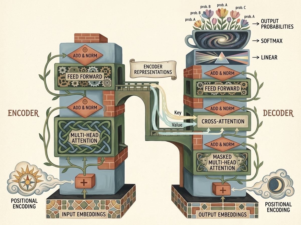
In Cross-Attention:
- The Queries ($Q$) originate from the Decoder’s previous layer: $Q = X_{\text{dec}} W_Q$.
- The Keys ($K$) and Values ($V$) originate from the final output representations of the Encoder: $K = H_{\text{enc}} W_K, \quad V = H_{\text{enc}} W_V$.
- The decoder dynamically attends to relevant source tokens regardless of their position in the source sentence.
9. Tokenization Paradigms & Autoregressive Decoding
9.1 Subword Tokenization: BPE & WordPiece
While character-level modeling is pedagogically pristine, modeling human language character by character results in long sequences: a 500-word paragraph spans 3,000 characters. Because self-attention has $O(T^2)$ memory and compute complexity, character-level processing becomes computationally prohibitive for books and long contexts.
Modern LLMs utilize Subword Tokenization:
- Byte Pair Encoding (BPE): Iteratively merges the most frequent pairs of bytes or characters in a training corpus until a predefined vocabulary size (typically 32,000 to 128,000 tokens) is reached.
- Common words like
"the"or"learning"become single tokens. Rare words like"translatability"decompose into meaningful subword chunks:["trans", "lat", "ability"].
9.2 Autoregressive Text Generation Strategies
During inference, given a prompt sequence $x_{1:t}$, the model produces output logits $\mathbf{z}_{t+1} \in \mathbb{R}^{|\mathcal{V}|}$. How do we sample the next token?
@torch.inference_mode()
def generate(model, prompt, max_new_tokens=20, temperature=1.0, top_k=None):
"""
Autoregressive generation loop with temperature scaling and Top-K truncation.
"""
model.eval()
idx = prompt # Shape: (1, T)
for _ in range(max_new_tokens):
# Crop context if it exceeds model block size
idx_cond = idx[:, -model.block_size:] if idx.size(1) > model.block_size else idx
# Forward pass to retrieve next-token logits
logits, _ = model(idx_cond)
logits = logits[:, -1, :] / max(temperature, 1e-5) # Scale by temperature
# Optional Top-K truncation
if top_k is not None:
v, _ = torch.topk(logits, min(top_k, logits.size(-1)))
logits[logits < v[:, [-1]]] = -float('Inf')
probs = F.softmax(logits, dim=-1)
next_idx = torch.multinomial(probs, num_samples=1)
# Append new token to sequence
idx = torch.cat((idx, next_idx), dim=1)
# Terminate early if sentinel is generated
if next_idx.item() == stoi[special_char]:
break
return idx
- Greedy Search ($T \to 0$): Always picks $x_{t+1} = \arg\max_i z_i$. Highly deterministic, but prone to repetitive loops and degenerate phrasing.
- Temperature Scaling ($T > 0$): Modulates probability entropy via $P(x_i) = \frac{e^{z_i / T}}{\sum_j e^{z_j / T}}$. $T < 1.0$ sharpens confidence onto high-probability modes; $T > 1.0$ flattens the distribution, injecting creative variance.
- Top-K Truncation: Filters out all tokens outside the $K$ highest-probability candidates before sampling, eliminating erratic tail tokens.
- Top-P (Nucleus) Sampling: Accumulates tokens in decreasing probability order until their cumulative sum reaches probability threshold $p$ (e.g., $p=0.90$), dynamically adapting the candidate pool size based on model confidence.
10. Computer Vision Meets Transformers: The Vision Transformer (ViT)
In 2020, Dosovitskiy et al. published the landmark paper “An Image is Worth 16x16 Words: Transformers for Image Recognition at Scale”, demonstrating that pure Transformer architectures can outperform state-of-the-art CNNs on computer vision benchmarks.
10.1 Image Patch Extraction as Tokenization
How do we feed a 2D continuous pixel tensor $\mathbf{x} \in \mathbb{R}^{H \times W \times C}$ into a 1D Transformer sequence model? The Vision Transformer partitions the image into a grid of non-overlapping square patches of spatial resolution $P \times P$ (typically $16 \times 16$ or $14 \times 14$):
$$ N = \frac{H \cdot W}{P^2} $$

For a standard ImageNet input of $224 \times 224$ RGB image with patch size $P=16$:
- Number of patches: $N = \frac{224 \times 224}{16 \times 16} = 14 \times 14 = 196$ patches.
- Raw patch vector length: $P^2 \cdot C = 16 \times 16 \times 3 = 768$.
In PyTorch, rather than manually slicing tensor loops, patch extraction and linear projection are computed in a single GPU operation using a 2D convolution whose kernel_size and stride are both equal to patch size $P$:
# Optimal PyTorch patch projection using strided 2D convolution
patch_size = 16
in_channels = 3
d_model = 768
patch_proj = nn.Conv2d(
in_channels=in_channels,
out_channels=d_model,
kernel_size=patch_size,
stride=patch_size
)
# Test with standard input batch: (B=1, C=3, H=224, W=224)
dummy_img = torch.randn(1, 3, 224, 224)
projected_patches = patch_proj(dummy_img) # Shape: (1, 768, 14, 14)
# Flatten spatial dimensions into token sequence: (B, N, d_model)
tokens = projected_patches.flatten(2).transpose(1, 2)
print(f"ViT Token Sequence Shape: {tokens.shape} -> (Batch=1, N=196, d_model=768)")
10.2 The Complete ViT Pipeline

- The Prepended
[CLS]Token: Following BERT convention, ViT prepends a learnable classification parameter token $\mathbf{x}{\text{class}} \in \mathbb{R}^{1 \times 1 \times d{\text{model}}}$ to the patch sequence, expanding the sequence length from $N$ to $N+1 = 197$. Because self-attention allows all-to-all information routing, $\mathbf{x}_{\text{class}}$ aggregates holistic visual representations from all patches across layers without favoring any specific spatial coordinate. - 1D Learnable Positional Embeddings: Transformers have zero inherent awareness of spatial geometry. To encode 2D spatial layout, a learnable positional embedding matrix $E_{\text{pos}} \in \mathbb{R}^{1 \times (N+1) \times d_{\text{model}}}$ is added elementwise: $$ \mathbf{z}0 = [\mathbf{x}{\text{class}}; , \mathbf{x}_p^1 E; , \dots; , \mathbf{x}p^N E] + E{\text{pos}} $$
- Transformer Encoder Processing: The resulting sequence passes through $L$ standard bidirectional Transformer Encoder blocks (LayerNorm, Multi-Head Attention, MLP).
- Classification Head: The representation of the
[CLS]token at layer $L$ ($\mathbf{z}_L^0$) is extracted, normalized via LayerNorm, and passed through a final linear layer to predict class logits: $$ \mathbf{y} = \text{Linear}(\text{LayerNorm}(\mathbf{z}_L^0)) $$
10.3 Inductive Biases: CNNs vs. Vision Transformers
| Dimension | Convolutional Neural Networks (CNNs) | Vision Transformers (ViTs) |
|---|---|---|
| Inherent Inductive Biases | High: Translation equivariance & spatial locality hardcoded into kernel operations | Minimal: Zero built-in spatial bias; must learn 2D relationships purely from data |
| Receptive Field Growth | Expands linearly or logarithmically with depth | Global ($O(1)$) from the very first layer |
| Data Efficiency on Small Datasets | Strong performance on small datasets (ImageNet-1K) | Prone to overfitting on small datasets without heavy regularization |
| Scaling Ceiling at Massive Scale | Performance saturates as dataset scales to $>100\text{M}$ images | Continues scaling log-linearly without saturation (JFT-300M, ImageNet-22K) |
11. Computational Complexity & Memory Profiling
Understanding the compute and memory profile of the Transformer architecture is crucial for systems engineering:
11.1 Self-Attention Quadratic Scaling
Let $T$ denote sequence length and $d$ denote embedding dimension:
- Projection Matrices ($Q, K, V$): Computing $X W_Q, X W_K, X W_V$ requires $3 \times (T \cdot d \cdot d) = 3 T d^2$ FLOPs.
- Attention Score Matrix ($Q K^T$): Multiplying $(T \times d)$ by $(d \times T)$ requires $T^2 d$ FLOPs.
- Softmax Normalization: Computing exponentials and row sums requires $O(T^2)$ operations.
- Value Aggregation ($A V$): Multiplying $(T \times T)$ attention matrix by $(T \times d)$ requires $T^2 d$ FLOPs.
- Output Projection: Multiplying by $W_O$ requires $T d^2$ FLOPs.
$$ \text{Total Self-Attention FLOPs} \approx 4 T d^2 + 2 T^2 d $$
Architectural Bottleneck: When context length $T \gg d$, the $2 T^2 d$ term dominates. In contemporary LLMs extending to 32K or 128K context windows, naive attention matrix storage requires $T \times T \times \text{heads} \times 2\text{ bytes}$ of VRAM, which triggered the invention of memory-efficient GPU kernel fusions like FlashAttention-2 (Dao, 2023).
12. Summary & Key Takeaways
- The Fundamental Shift: Transformers replaced recurrent sequential dependencies ($O(N)$ path length) with self-attention ($O(1)$ pairwise path length), unlocking full GPU tensor parallelism.
- Self-Supervised Autoregressive Formulation: Training language models requires no human annotations; raw text sequences are sliced into expanding causal prefixes paired with immediate next-token labels.
- Scaled Dot-Product Necessity: Dividing query-key dot products by $\sqrt{d_k}$ prevents logits from entering extreme softmax saturation where gradients vanish.
- Causal Masking: Adding an upper-triangular $-\infty$ mask ensures autoregressive decoders cannot peek into future tokens during training.
- Layer Normalization Independence: Unlike Batch Normalization which computes statistics across samples and breaks on variable-length text, Layer Normalization computes statistics across feature channels per token, operating identically during training and inference.
- Vision Transformers (ViT): By partitioning 2D images into $P \times P$ pixel patches and projecting them linearly into 1D token embeddings, Transformers achieve state-of-the-art computer vision performance with minimal inductive bias.
Diffusion Models for Images
- 1. The Generative Vision Paradigm: From VAEs and GANs to Diffusion
- 2. The Modern Diffusion Revolution (DALL-E & Stable Diffusion)
- 3. Core Working Principle: Diffusion in Three Stages
- 4. Pedagogical Setup: 2D Point Cloud Contour (PyTorch Logo)
- 5. The Forward Diffusion Process: Systematic Destruction of Data
- 6. Learning to Reverse the Arrow of Time: Model Architecture & Training
- 7. Reversing the Diffusion Process: The DDPM Sampling Algorithm
- 8. Scaling from 2D Points to Real-World Images (U-Net & Latent Diffusion)
- 9. Exercises & Complete Analytical Solutions
- 10. Chapter Summary & Key Takeaways
1. The Generative Vision Paradigm: From VAEs and GANs to Diffusion
Generative artificial intelligence in computer vision seeks to solve a fundamentally inverse problem: given a high-dimensional collection of real-world observations (images), how can an algorithm model the true underlying probability distribution $p_{\text{data}}(\mathbf{x})$ such that drawing a new sample produces a novel, visually coherent, and physically plausible scene?
In the preceding chapter on sequence modeling and transformers, tokens exhibited sequential dependencies where probability distributions factorized autoregressively across one-dimensional timelines:
$$ p(\mathbf{w}) = \prod_{i=1}^N p(w_i \mid w_1, w_2, \dots, w_{i-1}) $$
Image generation defies trivial autoregressive ordering. An image $\mathbf{x} \in \mathbb{R}^{C \times H \times W}$ is an array of spatially correlated pixels where local patches, semantic boundaries, global illumination, and high-frequency textures exert mutual, non-causal constraints simultaneously in two-dimensional space. Historically, two generative paradigms dominated image synthesis prior to the advent of diffusion: Variational Autoencoders (VAEs) and Generative Adversarial Networks (GANs).
flowchart TD
subgraph VAEFlow ["Variational Autoencoder (VAE) Pipeline"]
direction TB
V1["Input Image (X)<br/>(Pixel Space: C x H x W)"] --> V2["Encoder Network<br/>q_phi(z | x)"]
V2 --> V3["Latent Distribution<br/>(mu_z, sigma_z)"]
V3 --> V4["Latent Vector (z)<br/>z ~ N(mu, sigma^2)"]
V4 --> V5["Decoder Network<br/>p_theta(x | z)"]
V5 --> V6["Reconstructed Image (X')<br/>Reconstruction + KL Loss"]
end
subgraph GANFlow ["Generative Adversarial Network (GAN) Pipeline"]
direction TB
G1["Gaussian Noise (z)<br/>z ~ N(0, I)"] --> G2["Generator Network (G)<br/>G_theta(z)"]
G2 --> G3["Synthetic Candidate (X')"]
G4["Real Dataset Sample (X)"] --> G5["Discriminator Network (D)<br/>D_phi(x) -> [0, 1]"]
G3 --> G5
G5 --> G6["Minimax Adversarial Game<br/>min_G max_D V(D, G)"]
end
style VAEFlow fill:#1a1a2e,stroke:#4cc9f0,stroke-width:2px,color:#fff
style GANFlow fill:#16213e,stroke:#f72585,stroke-width:2px,color:#fff
1.1 Variational Autoencoders (VAEs)
Introduced by Kingma and Welling in late 2013, the Variational Autoencoder (VAE) formulates generation as probabilistic latent-variable inference. An encoder network $q_\phi(\mathbf{z} \mid \mathbf{x})$ maps high-dimensional pixels into parameters of a multivariate Gaussian distribution over an unobserved low-dimensional latent space $\mathbf{z} \in \mathbb{R}^d$:
$$ q_\phi(\mathbf{z} \mid \mathbf{x}) = \mathcal{N}\left(\mathbf{z};, \boldsymbol{\mu}_\phi(\mathbf{x}),, \operatorname{diag}(\boldsymbol{\sigma}_\phi^2(\mathbf{x}))\right) $$
A decoder network $p_\theta(\mathbf{x} \mid \mathbf{z})$ reconstructs the input image from a stochastic sample drawn via the reparameterization trick $\mathbf{z} = \boldsymbol{\mu} + \boldsymbol{\sigma} \odot \boldsymbol{\epsilon}$, where $\boldsymbol{\epsilon} \sim \mathcal{N}(\mathbf{0}, \mathbf{I})$. Training optimizes the Evidence Lower Bound (ELBO):
$$ \log p(\mathbf{x}) \ge \mathbb{E}_{q_\phi(\mathbf{z} \mid \mathbf{x})}\left[\log p_\theta(\mathbf{x} \mid \mathbf{z})\right] - D_{\text{KL}}\left(q_\phi(\mathbf{z} \mid \mathbf{x}) \parallel p(\mathbf{z})\right) $$
To synthesize brand-new imagery, the encoder is discarded: random vector $\mathbf{z} \sim \mathcal{N}(\mathbf{0}, \mathbf{I})$ is passed directly into the decoder. While theoretically elegant and stable to train, VAEs suffer from a well-documented flaw: reconstructed and sampled images frequently exhibit blurriness and lack sharp textural fidelity because the pixel-wise mean squared error (MSE) or Gaussian log-likelihood rewards averaging over ambiguous high-frequency configurations.
1.2 Generative Adversarial Networks (GANs)
In 2014, Goodfellow et al. introduced Generative Adversarial Networks (GANs), bypassing explicit density estimation entirely in favor of a two-player zero-sum minimax game:
$$ \min_G \max_D V(D, G) = \mathbb{E}_{\mathbf{x} \sim p_{\text{data}}(\mathbf{x})}\left[\log D(\mathbf{x})\right] + \mathbb{E}_{\mathbf{z} \sim p_{\mathbf{z}}(\mathbf{z})}\left[\log(1 - D(G(\mathbf{z})))\right] $$
The Generator $G_\theta$ maps random noise $\mathbf{z} \sim \mathcal{N}(\mathbf{0}, \mathbf{I})$ into synthetic images $G(\mathbf{z})$. The Discriminator $D_\phi$ acts as a binary classifier, determining whether a given image originated from the authentic empirical dataset or the generator’s synthetic distribution.
Through simultaneous gradient updates, GANs produce breathtakingly crisp, photorealistic edges. However, their training dynamics are notoriously fragile:
- Mode Collapse: The generator discovers a minuscule subset of plausible visual outputs that reliably deceive the discriminator, completely ignoring the rich variety of the real distribution.
- Vanishing Gradients & Nash Equilibrium Instability: When the discriminator achieves near-perfect classification early in training, gradients driving generator optimization vanish or oscillate wildly.
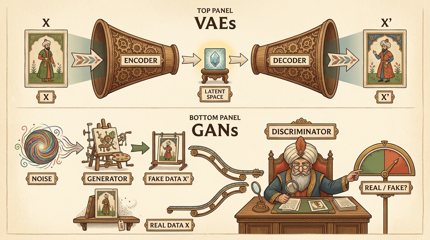
2. The Modern Diffusion Revolution (DALL-E & Stable Diffusion)
In 2015, Jascha Sohl-Dickstein et al. (Deep Unsupervised Learning Using Nonequilibrium Thermodynamics) proposed a radically different approach inspired by physical diffusion. Rather than attempting to map arbitrary noise to an image in a single monolithic forward pass (as in GANs), they proposed systematically destroying data structure through a slow, progressive degradation process, and subsequently training a deep neural network to reverse that degradation step by step.
While initially overshadowed by GANs, diffusion models experienced an exponential breakthrough between 2020 and 2022 following Jonathan Ho, Ajay Jain, and Pieter Abbeel’s landmark paper, Denoising Diffusion Probabilistic Models (DDPM). Ho et al. showed that with reparameterized objectives and U-Net backbones, diffusion models systematically outperform GANs in visual sample fidelity and sample diversity without adversarial instability.
Commercial systems rapidly materialized:
- DALL-E 2 (OpenAI): Scaled conditional diffusion for high-fidelity cross-modal text-to-image synthesis.
- Stable Diffusion / SDXL (CompVis, Runway, Stability AI): Latent Diffusion Models (LDMs) that project diffusion onto low-dimensional autoencoded latent manifolds, enabling real-time, desktop-class generation of 1024x1024 photorealistic imagery.
flowchart TD
subgraph GenTimeline ["Evolution of Generative Vision Architectures"]
direction TB
T1["2013: Variational Autoencoders (VAEs)<br/>Stable ELBO optimization, but blurry outputs"]
T2["2014: Generative Adversarial Networks (GANs)<br/>Crisp visual boundaries, but severe mode collapse"]
T3["2015: Nonequilibrium Thermodynamics (Sohl-Dickstein)<br/>First formulation of iterative forward/reverse diffusion"]
T4["2020: Denoising Diffusion Probabilistic Models (DDPM)<br/>Reparameterized MSE noise prediction beats GANs"]
T5["2022+: Latent Diffusion Models & Stable Diffusion (SDXL)<br/>Scalable text-conditioned synthesis on latent representations"]
T1 --> T2 --> T3 --> T4 --> T5
end
style GenTimeline fill:#0f3460,stroke:#e94560,stroke-width:2px,color:#fff
3. Core Working Principle: Diffusion in Three Stages
The foundational engineering paradigm behind generative diffusion models decomposes into three distinct phases:
- Forward Process (Systematic Perturbation): Starting from clean empirical data ($\mathbf{x}_0$), we inject small, controlled increments of Gaussian noise across discrete timesteps ($t = 1, \dots, T$). After sufficient degradation steps (e.g., $T = 1000$), the original structural information is entirely erased, yielding pure isotropic Gaussian noise ($\mathbf{x}_T \sim \mathcal{N}(\mathbf{0}, \mathbf{I})$).
- Training Phase (Noise Estimation): A deep neural network is trained to observe a perturbed sample $\mathbf{x}_t$ at any arbitrary timestep $t$ and answer a single question: “What was the exact noise vector $\boldsymbol{\epsilon}$ injected into this state?” Rather than attempting to predict the clean high-dimensional image directly, the network predicts the additive noise perturbation.
- Reverse Sampling Phase (Generative Synthesis): To synthesize novel data from scratch, we sample pure noise from a standard normal distribution ($\mathbf{x}_T$). The trained network iteratively estimates and subtracts the noise perturbation step by step ($t = T \to 0$). As noise is progressively removed, pristine, coherent visual data emerges from initial entropy.
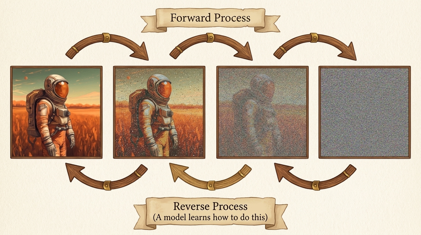
4. Pedagogical Setup: 2D Point Cloud Contour (PyTorch Logo)
To build intuition without the multi-gigabyte memory overhead and lengthy training cycles of 2D convolutional networks over ImageNet, this chapter begins by modeling a two-dimensional geometric manifold: the outline coordinates of the PyTorch Logo.
An arbitrary image $\mathbf{x} \in \mathbb{R}^{H \times W \times C}$ is simply a collection of localized scalar measurements. Similarly, a 2D contour is a set of $N$ coordinate pairs $\mathbf{x} = (p_0, p_1) \in \mathbb{R}^2$. Applying diffusion to 2D coordinates demonstrates every single mathematical identity, variance schedule, noise calculation, closed-form jump, and sampling algorithm identically to high-resolution diffusion models like SDXL.
4.1 Extracting 2D Contour Coordinates from Logo Image
Before executing diffusion, we extract boundary points from the official PyTorch logo image. The logo can be downloaded directly from a high-resolution transparent PNG URL, resized to $256 \times 256$, and contour points extracted via edge filtering or alpha masking:
import io
import urllib.request
import numpy as np
import torch
import torch.nn as nn
import torch.nn.functional as F
import matplotlib.pyplot as plt
from PIL import Image, ImageFilter
# Action 1: Set device and deterministic seed for reproducible geometry
device = torch.device("cuda" if torch.cuda.is_available() else "cpu")
torch.manual_seed(42)
np.random.seed(42)
print(f"Active Compute Device: {device}")
We define an extraction utility that loads the logo image from an online URL or local file, resizes it to $256 \times 256$, identifies opaque boundary edges using Sobel/edge filtering, centers the coordinates at the origin $(0, 0)$, and normalizes their variance to unit scale ($1.0$):
# Action 2: Define image/URL to 2D point extraction utility
def load_pytorch_logo_points(
source="https://res.cloudinary.com/startup-grind/image/upload/c_fill,w_500,h_500,g_center/c_fill,dpr_2.0,f_auto,g_center,q_auto:good/v1/gcs/platform-data-linuxhq/events/PyTorch_Symbol_01_OrangeOnTransparent_nUWxXkQ.png",
num_points=3000,
target_size=(256, 256),
):
"""
Downloads or loads a PyTorch logo PNG, resizes to target_size (256x256),
extracts visual edge contours, and normalizes points to zero mean & unit variance.
"""
try:
if source.startswith("http://") or source.startswith("https://"):
req = urllib.request.Request(source, headers={"User-Agent": "Mozilla/5.0"})
with urllib.request.urlopen(req, timeout=10) as resp:
img_bytes = resp.read()
img = Image.open(io.BytesIO(img_bytes)).convert("RGBA")
else:
img = Image.open(source).convert("RGBA")
except Exception as err:
print(f"URL loading failed ({err}). Generating parametric fallback logo...")
# Parametric synthetic fallback (flame & ring)
theta = np.linspace(0, 2 * np.pi, int(num_points * 0.65), endpoint=False)
ring_x, ring_y = 1.8 * np.cos(theta), 1.8 * np.sin(theta)
flame_pts = int(num_points * 0.35)
flame_x = np.concatenate([np.linspace(-0.5, 0.5, flame_pts // 2), np.zeros(flame_pts - flame_pts // 2)])
flame_y = np.concatenate([np.linspace(-1.0, 1.2, flame_pts // 2), np.linspace(0.2, 1.5, flame_pts - flame_pts // 2)])
coords = np.stack([np.concatenate([ring_x, flame_x]), np.concatenate([ring_y, flame_y])], axis=1).astype(np.float32)
coords -= coords.mean(axis=0, keepdims=True)
coords /= coords.std()
return torch.tensor(coords, dtype=torch.float32)
# Resize to specified dimensions (256 x 256)
img = img.resize(target_size, Image.Resampling.LANCZOS)
# Extract edge contours using Sobel/FIND_EDGES filter
gray = img.convert("L")
edges = gray.filter(ImageFilter.FIND_EDGES)
edge_array = np.array(edges)
# Locate coordinates where edge intensity exceeds threshold
y_indices, x_indices = np.where(edge_array > 40)
total_found = len(x_indices)
# If edge detection yields few points, fall back to alpha mask pixels
if total_found < 500:
alpha = np.array(img)[:, :, 3]
y_indices, x_indices = np.where(alpha > 50)
total_found = len(x_indices)
chosen_indices = np.random.choice(total_found, num_points, replace=(total_found < num_points))
x_pts = x_indices[chosen_indices].astype(np.float32)
y_pts = -y_indices[chosen_indices].astype(np.float32) # Invert Y to match Cartesian plane
coords = np.stack([x_pts, y_pts], axis=1)
coords -= coords.mean(axis=0, keepdims=True)
coords /= np.std(coords) # Unit variance normalization
return torch.tensor(coords, dtype=torch.float32)
When visual contours are loaded and converted into a PyTorch floating-point tensor, the dataset tensor $\mathbf{x}_0$ exhibits shape $(N, 2)$:
# Action 3: Load PyTorch logo points (from URL / local file) into PyTorch tensor
LOGO_URL = "https://res.cloudinary.com/startup-grind/image/upload/c_fill,w_500,h_500,g_center/c_fill,dpr_2.0,f_auto,g_center,q_auto:good/v1/gcs/platform-data-linuxhq/events/PyTorch_Symbol_01_OrangeOnTransparent_nUWxXkQ.png"
x0 = load_pytorch_logo_points(source=LOGO_URL, num_points=3000, target_size=(256, 256))
print(f"Dataset x0 Tensor Shape: {x0.shape} | Mean: {x0.mean():.4f} | Std: {x0.std():.4f}")
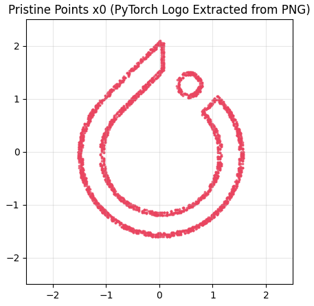
5. The Forward Diffusion Process: Systematic Destruction of Data
The forward diffusion process (also termed the noising process) gradually adds synthetic Gaussian perturbations to the ground-truth data $\mathbf{x}_0$ over a discrete sequence of $T$ timesteps, producing a trajectory of increasingly noisy latent variables $\mathbf{x}_1, \mathbf{x}_2, \dots, \mathbf{x}_T$.
flowchart TD
subgraph ForwardMarkov ["Forward Diffusion Markov Chain (q)"]
direction TB
M0["Pristine Data (x0)<br/>p(x0) ~ Empirical Data"]
M1["Timestep 1 (x1)<br/>Slightly degraded"]
M2["Timestep 2 (x2)"]
Mt["Timestep t (xt)"]
MT["Timestep T (xT)<br/>Isotropic Gaussian N(0, I)"]
M0 --> M1
M1 --> M2
M2 --> Mt
Mt --> MT
end
style ForwardMarkov fill:#1a1a2e,stroke:#52b788,stroke-width:2px,color:#fff
5.1 Step-by-Step Markovian Perturbation
The forward process is modeled as a Markov chain where each transition $q(\mathbf{x}_t \mid \mathbf{x}_{t-1})$ depends solely on the immediately preceding state $\mathbf{x}_{t-1}$. Each step injects a small amount of Gaussian noise controlled by a scalar variance parameter $\beta_t \in (0, 1)$:
$$ q(\mathbf{x}_t \mid \mathbf{x}_{t-1}) = \mathcal{N}\left(\mathbf{x}_t;, \sqrt{1 - \beta_t},\mathbf{x}_{t-1},, \beta_t \mathbf{I}\right) $$
Notice the critical scaling factor $\sqrt{1 - \beta_t}$ applied to the mean. Why is this scaling term necessary? If we simply added noise without scaling down the prior data ($\mathbf{x}_t = \mathbf{x}_{t-1} + \sqrt{\beta_t}\boldsymbol{\epsilon}$), the variance of $\mathbf{x}_t$ would grow unboundedly with each timestep ($\operatorname{Var}(\mathbf{x}_t) = \operatorname{Var}(\mathbf{x}_{t-1}) + \beta_t$). By weighting the prior state by $\sqrt{1 - \beta_t}$, the total variance is preserved at unit scale across all steps:
$$ \operatorname{Var}(\mathbf{x}_t) = (1 - \beta_t)\operatorname{Var}(\mathbf{x}_{t-1}) + \beta_t \operatorname{Var}(\boldsymbol{\epsilon}) = (1 - \beta_t)(1) + \beta_t(1) = 1 $$
5.2 Variance Schedules: Linear Beta Schedule
The sequence $\beta_1, \beta_2, \dots, \beta_T$ is determined by a predefined noise schedule. In this chapter, we use a standard linear schedule starting from $\beta_1 = 10^{-4}$ and increasing linearly to $\beta_T = 0.02$ across $T = 1000$ timesteps:
$$ \beta_t = \beta_1 + \frac{t - 1}{T - 1}(\beta_T - \beta_1) $$
# Action 1: Construct the linear beta variance schedule
def linear_beta_schedule(timesteps=1000, start=0.0001, end=0.02):
"""
Generates a linearly spaced 1D tensor of beta values controlling
the variance of injected noise across discrete timesteps.
"""
return torch.linspace(start, end, timesteps)
T = 1000
betas = linear_beta_schedule(timesteps=T)
print(f"Beta Schedule: beta_0 = {betas[0]:.6f} | beta_500 = {betas[500]:.6f} | beta_999 = {betas[-1]:.6f}")
Applying this transition iteratively for one step:
# Action 2: Single-step Markovian forward perturbation
def diffuse_single_step(points, beta):
"""
Applies one discrete step of Markovian Gaussian diffusion q(x_t | x_{t-1}).
"""
# Scale down prior state
new_mean = torch.sqrt(1.0 - beta) * points
# Sample standard normal noise
noise = torch.randn_like(points)
# Scale perturbation by sqrt(beta)
perturbation = torch.sqrt(beta) * noise
return new_mean + perturbation, noise
5.3 Closed-Form Analytical Jump: Eliminating Iterative Loops
If training a neural network required executing a sequential loop of 800 forward steps just to compute the noisy state $\mathbf{x}_{800}$ for an image, backpropagation would be impossibly slow and memory-prohibitive.
Remarkably, because the sum of independent Gaussian random variables is itself Gaussian, the entire chain $q(\mathbf{x}_1 \mid \mathbf{x}_0) \dots q(\mathbf{x}_t \mid \mathbf{x}_{t-1})$ can be collapsed into a closed-form analytical jump that calculates $\mathbf{x}_t$ directly from $\mathbf{x}_0$ in a single operation.
Let $\alpha_t = 1 - \beta_t$, and define the cumulative product:
$$ \bar{\alpha}_t = \prod_{s=1}^t \alpha_s $$
Let us expand $\mathbf{x}_t$ recursively using reparameterized noise terms $\boldsymbol{\epsilon}_0, \boldsymbol{\epsilon}_1, \dots \sim \mathcal{N}(\mathbf{0}, \mathbf{I})$:
$$ \mathbf{x}_t = \sqrt{\alpha_t}\mathbf{x}_{t-1} + \sqrt{1 - \alpha_t}\boldsymbol{\epsilon}_{t-1} $$
Substitute $\mathbf{x}_{t-1} = \sqrt{\alpha_{t-1}}\mathbf{x}_{t-2} + \sqrt{1 - \alpha_{t-1}}\boldsymbol{\epsilon}_{t-2}$:
$$ \mathbf{x}_t = \sqrt{\alpha_t}\left(\sqrt{\alpha_{t-1}}\mathbf{x}_{t-2} + \sqrt{1 - \alpha_{t-1}}\boldsymbol{\epsilon}_{t-2}\right) + \sqrt{1 - \alpha_t}\boldsymbol{\epsilon}_{t-1} $$ $$ \mathbf{x}_t = \sqrt{\alpha_t \alpha_{t-1}}\mathbf{x}_{t-2} + \sqrt{\alpha_t(1 - \alpha_{t-1})}\boldsymbol{\epsilon}_{t-2} + \sqrt{1 - \alpha_t}\boldsymbol{\epsilon}_{t-1} $$
The two Gaussian noise terms $\sqrt{\alpha_t(1 - \alpha_{t-1})}\boldsymbol{\epsilon}_{t-2}$ and $\sqrt{1 - \alpha_t}\boldsymbol{\epsilon}_{t-1}$ are independent. Recall that for independent Gaussians $\mathcal{N}(\mathbf{0}, \sigma_1^2 \mathbf{I}) + \mathcal{N}(\mathbf{0}, \sigma_2^2 \mathbf{I}) \sim \mathcal{N}(\mathbf{0}, (\sigma_1^2 + \sigma_2^2)\mathbf{I})$. Summing their variances:
$$ \alpha_t(1 - \alpha_{t-1}) + (1 - \alpha_t) = \alpha_t - \alpha_t \alpha_{t-1} + 1 - \alpha_t = 1 - \alpha_t \alpha_{t-1} $$
Thus, the two noise terms collapse into a single standard Gaussian $\sqrt{1 - \alpha_t \alpha_{t-1}}\bar{\boldsymbol{\epsilon}}$. Unrolling this induction all the way to $\mathbf{x}_0$:
$$ \mathbf{x}_t = \sqrt{\bar{\alpha}_t}\mathbf{x}_0 + \sqrt{1 - \bar{\alpha}_t}\boldsymbol{\epsilon}, \quad \text{where } \boldsymbol{\epsilon} \sim \mathcal{N}(\mathbf{0}, \mathbf{I}) $$
$$ q(\mathbf{x}_t \mid \mathbf{x}_0) = \mathcal{N}\left(\mathbf{x}_t;, \sqrt{\bar{\alpha}_t}\mathbf{x}_0,, (1 - \bar{\alpha}_t)\mathbf{I}\right) $$
Practical Anatomy of the Closed-Form Equation
This formula directly balances two complementary components:
- $\sqrt{\bar{\alpha}_t}\mathbf{x}_0$: Original Signal Contribution. As timestep $t$ increases, cumulative product $\bar{\alpha}_t \to 0$, diminishing the weight of pristine data $\mathbf{x}_0$.
- $\sqrt{1 - \bar{\alpha}_t}\boldsymbol{\epsilon}$: Injected Noise Contribution. As $t$ increases, $1 - \bar{\alpha}_t \to 1$, making random noise increasingly dominant.
- Because the sum of their squared coefficients $(\sqrt{\bar{\alpha}_t})^2 + (\sqrt{1 - \bar{\alpha}_t})^2 = \bar{\alpha}_t + 1 - \bar{\alpha}_t = 1$, the total variance remains preserved at exactly $1.0$ across all timesteps.
Key Insight: At any arbitrary timestep $t \in [1, T]$, we can sample noisy state $\mathbf{x}_t$ directly in $\mathcal{O}(1)$ time without traversing intermediate timesteps $1, 2, \dots, t-1$. During training, this allows instantaneous sampling of arbitrary noise levels for any training batch.
5.4 PyTorch Implementation of the Closed-Form Forward Sampler
We precompute $\alpha_t$, $\bar{\alpha}_t$, $\sqrt{\bar{\alpha}_t}$, and $\sqrt{1 - \bar{\alpha}_t}$ on the appropriate device:
# Action 1: Precompute analytical diffusion coefficients
alphas = 1.0 - betas
alphas_cumprod = torch.cumprod(alphas, dim=0)
alphas_cumprod_prev = F.pad(alphas_cumprod[:-1], (1, 0), value=1.0)
sqrt_alphas_cumprod = torch.sqrt(alphas_cumprod)
sqrt_one_minus_alphas_cumprod = torch.sqrt(1.0 - alphas_cumprod)
# Action 2: Helper method for broadcasting 1D schedule values into N-D tensor shapes
def reshape_for_x(a, x):
"""
Extracts the values of 1D tensor `a` indexed by timestep, and reshapes it
to match the dimensionality of `x` with trailing singleton dimensions for broadcasting.
"""
batch_size = x.shape[0]
ones_to_broadcast = len(x.shape) - 1
return a.view(batch_size, *([1] * ones_to_broadcast)).to(x.device)
# Action 3: Closed-form single-step forward sampling function
def forward_diffusion_sample(x0, t, device=device):
"""
Samples x_t ~ q(x_t | x_0) in closed form using precomputed cumulative variance terms.
Returns noisy tensor x_t and the exact ground-truth noise epsilon injected.
"""
x0 = x0.to(device)
noise = torch.randn_like(x0)
# Extract coefficients for the specified batch of timesteps
sqrt_alpha_bar = reshape_for_x(sqrt_alphas_cumprod[t], x0)
sqrt_one_minus_alpha_bar = reshape_for_x(sqrt_one_minus_alphas_cumprod[t], x0)
# Analytical linear combination
xt = sqrt_alpha_bar * x0 + sqrt_one_minus_alpha_bar * noise
return xt, noise

6. Learning to Reverse the Arrow of Time: Model Architecture & Training
6.1 Objective: Estimating Injected Noise
To generate data, we must invert the forward process: given noisy state $\mathbf{x}_t$, we want to determine the previous, less-noisy state $\mathbf{x}_{t-1}$.
One might intuitively suppose our neural network should directly predict the clean image $\mathbf{x}_0$ from $\mathbf{x}_t$. However, Ho et al. (2020) demonstrated that parameterizing the network to predict the injected Gaussian noise vector $\boldsymbol{\epsilon}$ produces far superior empirical stability.
Why Predict the Noise Instead of the Image?
- Stationary Distribution Target: Ground-truth training images exhibit complex, multimodal, and diverse distributions. In contrast, the noise vector $\boldsymbol{\epsilon}$ always follows a fixed, symmetric standard normal distribution ($\mathcal{N}(\mathbf{0}, \mathbf{I})$) with zero mean and unit variance. Optimizing a neural network to predict values drawn from a standardized distribution stabilizes gradient dynamics.
- Instant Algebraic Recovery: Once the model predicts noise $\boldsymbol{\epsilon}_\theta(\mathbf{x}_t, t)$, an estimate of clean data $\mathbf{x}_0$ is recovered instantaneously through elementary algebra:
$$ \hat{\mathbf{x}}_0 = \frac{\mathbf{x}_t - \sqrt{1 - \bar{\alpha}_t}\boldsymbol{\epsilon}_\theta(\mathbf{x}_t, t)}{\sqrt{\bar{\alpha}_t}} $$
6.2 Sinusoidal Positional Embeddings
Because a single neural network must denoise inputs across all stages of degradation—from subtle noise at $t=1$ to near-pure entropy at $t=999$—the model must know what time $t$ it is operating on.
Passing a raw scalar $t \in [0, 999]$ directly into a linear layer performs poorly because deep networks struggle to learn high-frequency harmonic dependencies from raw unnormalized scalars. Instead, we use sinusoidal positional embeddings (Vaswani et al., 2017), which project scalar inputs across geometric frequency bands:
$$ \text{PE}(t, 2i) = \sin\left(\frac{t}{10000^{2i / d}}\right), \quad \text{PE}(t, 2i+1) = \cos\left(\frac{t}{10000^{2i / d}}\right) $$
# Action 1: Sinusoidal Positional Embedding Module
class SinusoidalEmbedding(nn.Module):
"""
Transforms continuous 1D coordinates or discrete timesteps into
high-dimensional sinusoidal representations across geometrically spaced frequencies.
"""
def __init__(self, dim):
super().__init__()
self.dim = dim
assert dim % 2 == 0, "Embedding dimension must be even."
def forward(self, x):
device = x.device
half_dim = self.dim // 2
# Precompute frequency scaling factors: 10000^(-2i / d)
emb_scale = torch.log(torch.tensor(10000.0, device=device)) / (half_dim - 1)
freqs = torch.exp(torch.arange(half_dim, device=device, dtype=torch.float32) * -emb_scale)
# Outer product of inputs with frequencies
args = x.view(-1, 1) * freqs.view(1, -1)
embedding = torch.cat([torch.sin(args), torch.cos(args)], dim=-1)
return embedding
def __len__(self):
return self.dim
6.3 The Denoising MLP Network Architecture
Our denoising architecture takes two coordinate inputs $(p_0, p_1)$ and timestep $t$. Each input is projected into a 128-dimensional sinusoidal feature representation, concatenated into a 384-dimensional feature vector, and passed through a three-layer Multi-Layer Perceptron (MLP) with ReLU non-linearities to output predicted noise $(\hat{\epsilon}_0, \hat{\epsilon}_1) \in \mathbb{R}^2$:
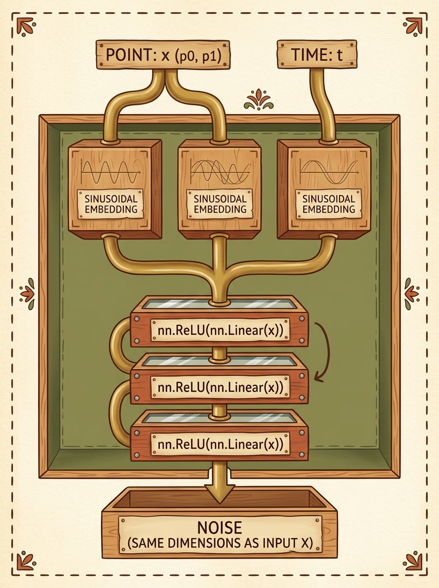
# Action 2: Denoising Neural Network with Sinusoidal Projections
class DenoisingModel(nn.Module):
"""
Predicts the noise perturbation epsilon injected into 2D coordinates at timestep t.
"""
def __init__(self, hidden_dim=128, num_layers=3):
super().__init__()
# Embeddings for x-coord, y-coord, and time
self.pos1_mlp = SinusoidalEmbedding(hidden_dim)
self.pos2_mlp = SinusoidalEmbedding(hidden_dim)
self.time_mlp = SinusoidalEmbedding(hidden_dim)
concat_dim = hidden_dim * 3
# Construct dense residual MLP backbone
layers = [nn.Linear(concat_dim, hidden_dim), nn.ReLU()]
for _ in range(num_layers):
layers.extend([nn.Linear(hidden_dim, hidden_dim), nn.ReLU()])
# Final projection back to 2D noise coordinate space
layers.append(nn.Linear(hidden_dim, 2))
self.joint_mlp = nn.Sequential(*layers)
def forward(self, x, t):
# x has shape (B, 2) where column 0 is p0 and column 1 is p1
x1_emb = self.pos1_mlp(x[:, 0])
x2_emb = self.pos2_mlp(x[:, 1])
t_emb = self.time_mlp(t.float())
# Concatenate multi-modal spatial and temporal representations
joint_features = torch.cat([x1_emb, x2_emb, t_emb], dim=-1)
predicted_noise = self.joint_mlp(joint_features)
return predicted_noise
6.4 The Simplified Training Objective ($L_{\text{simple}}$)
Ho et al. proved that variational bound optimization simplifies into an unweighted Mean Squared Error (MSE) loss measuring the distance between true injected noise $\boldsymbol{\epsilon}$ and network prediction $\boldsymbol{\epsilon}_\theta(\mathbf{x}_t, t)$:
$$ L_{\text{simple}}(\theta) = \mathbb{E}_{t, \mathbf{x}_0, \boldsymbol{\epsilon}} \left[ \left\Vert \boldsymbol{\epsilon} - \boldsymbol{\epsilon}_\theta\left(\sqrt{\bar{\alpha}_t}\mathbf{x}_0 + \sqrt{1 - \bar{\alpha}_t}\boldsymbol{\epsilon},, t\right) \right\Vert^2 \right] $$
# Action 3: Loss calculation function
def get_loss(model, x0, t, device=device):
"""
Computes L_simple(theta): MSE loss between actual injected noise and network estimate.
"""
xt, true_noise = forward_diffusion_sample(x0, t, device=device)
predicted_noise = model(xt, t)
return F.mse_loss(predicted_noise, true_noise)
6.5 The Complete Training Loop
In each optimization step, we draw an empirical batch $\mathbf{x}_0$, independently sample a random integer timestep $t \sim \operatorname{Uniform}({0, 1, \dots, T-1})$ for each sample, compute closed-form noisy samples $\mathbf{x}_t$, and backpropagate the MSE loss:
# Action 4: Instantiate model, optimizer, and execute training loop
model = DenoisingModel(hidden_dim=128, num_layers=3).to(device)
optimizer = torch.optim.Adam(model.parameters(), lr=0.001)
def train_diffusion(model, optimizer, x_data, num_epochs=5000, batch_size=512):
model.train()
num_samples = x_data.shape[0]
for epoch in range(1, num_epochs + 1):
# Sample random mini-batch of 2D contour points
indices = torch.randint(0, num_samples, (batch_size,))
batch_x0 = x_data[indices].to(device)
# Sample random discrete timesteps uniformly across [0, T-1]
batch_t = torch.randint(0, T, (batch_size,), device=device)
optimizer.zero_grad()
loss = get_loss(model, batch_x0, batch_t, device=device)
loss.backward()
optimizer.step()
if epoch % 1000 == 0 or epoch == 1:
print(f"Epoch {epoch:5d} / {num_epochs} | Denoising MSE Loss: {loss.item():.6f}")
# Execute training (5000 epochs completes in seconds on modern GPUs)
train_diffusion(model, optimizer, x0, num_epochs=5000)
7. Reversing the Diffusion Process: The DDPM Sampling Algorithm
7.1 Why Reverse Sampling Cannot Jump in a Single Step
While the forward process allows instantaneous closed-form evaluation from $\mathbf{x}_0$ to $\mathbf{x}_t$, the reverse generative process $p_\theta(\mathbf{x}_{t-1} \mid \mathbf{x}_t)$ requires iterative, step-by-step ancestral sampling from $t = T$ down to $t = 0$.
Why can we not take pure noise $\mathbf{x}_T \sim \mathcal{N}(\mathbf{0}, \mathbf{I})$ and jump directly to $\mathbf{x}_0$ in one shot? Because predicting $\mathbf{x}_0$ from pure Gaussian noise in a single step is an ill-posed multimodal problem: millions of distinct real images are equally consistent with a given noise realization. Attempting a single-step inversion yields a blurry average over all possible modes (analogous to blurry VAE outputs). Iterative sampling allows the stochastic Markov trajectory to gradually collapse ambiguity, choosing a specific mode and progressively synthesizing fine details.
7.2 The Analytical Reverse Transition Formulation
From Bayes’ rule conditioned on $\mathbf{x}_0$, the true posterior transition $q(\mathbf{x}_{t-1} \mid \mathbf{x}_t, \mathbf{x}_0)$ is Gaussian:
$$ q(\mathbf{x}_{t-1} \mid \mathbf{x}_t, \mathbf{x}_0) = \mathcal{N}\left(\mathbf{x}_{t-1};, \tilde{\boldsymbol{\mu}}_t(\mathbf{x}_t, \mathbf{x}_0),, \tilde{\beta}_t \mathbf{I}\right) $$
where the posterior variance $\tilde{\beta}_t$ is:
$$ \tilde{\beta}_t = \frac{1 - \bar{\alpha}_{t-1}}{1 - \bar{\alpha}_t} \beta_t $$
Substituting the model’s prediction $\boldsymbol{\epsilon}_\theta(\mathbf{x}_t, t)$ for true noise $\boldsymbol{\epsilon}$, the estimated posterior mean becomes:
$$ \boldsymbol{\mu}_\theta(\mathbf{x}_t, t) = \frac{1}{\sqrt{\alpha_t}} \left( \mathbf{x}_t - \frac{\beta_t}{\sqrt{1 - \bar{\alpha}_t}} \boldsymbol{\epsilon}_\theta(\mathbf{x}_t, t) \right) $$
To sample state $\mathbf{x}_{t-1}$ from state $\mathbf{x}_t$:
$$ \mathbf{x}_{t-1} = \frac{1}{\sqrt{\alpha_t}} \left( \mathbf{x}_t - \frac{\beta_t}{\sqrt{1 - \bar{\alpha}_t}} \boldsymbol{\epsilon}_\theta(\mathbf{x}_t, t) \right) + \sigma_t \mathbf{z} $$
Mechanics of the Reverse Step Equation
- Noise Subtraction: The predicted noise vector $\boldsymbol{\epsilon}_\theta$ is weighted and subtracted from current state $\mathbf{x}_t$ ($\mathbf{x}_t - \dots \boldsymbol{\epsilon}_\theta$).
- Rescaling: The remaining signal is scaled up by $1 / \sqrt{\alpha_t}$ to maintain unit variance balance.
- Stochastic Annealing ($\sigma_t \mathbf{z}$): For all steps $t > 1$, a tiny injection of fresh Gaussian noise ($\mathbf{z} \sim \mathcal{N}(\mathbf{0}, \mathbf{I})$) prevents mode collapse and allows the trajectory to explore rich details. At terminal step $t = 0$, this stochastic term is zeroed ($\mathbf{z} = \mathbf{0}$) to yield a pristine, deterministic reconstructed output.
flowchart TD
subgraph ReverseMarkov ["Reverse Generative Sampling Trajectory (p_theta)"]
direction TB
R0["Pure Noise (xT)<br/>xT ~ N(0, I)"]
R1["Intermediate Sample (x_T-1)"]
Rt["Intermediate Sample (xt)"]
R2["Intermediate Sample (x1)"]
Rclean["Synthesized Clean Data (x0)<br/>Pristine PyTorch Logo Contour"]
R0 --> R1
R1 --> Rt
Rt --> R2
R2 --> Rclean
end
style ReverseMarkov fill:#1a1a2e,stroke:#4cc9f0,stroke-width:2px,color:#fff
7.3 Step-by-Step Reconstruction from Pure Gaussian Noise
We implement the reverse sampling function and iterate backwards from $T-1$ down to 0:
# Action 1: Precompute posterior variance terms
sqrt_recip_alphas = torch.sqrt(1.0 / alphas)
posterior_variance = betas * (1.0 - alphas_cumprod_prev) / (1.0 - alphas_cumprod)
# Action 2: Single-step reverse sampling function
@torch.no_grad()
def sample_timestep(model, x, t):
"""
Computes reverse transition p_theta(x_{t-1} | x_t) given current noisy state x
and current discrete timestep tensor t.
"""
betas_t = reshape_for_x(betas[t], x)
sqrt_one_minus_alpha_bar_t = reshape_for_x(sqrt_one_minus_alphas_cumprod[t], x)
sqrt_recip_alpha_t = reshape_for_x(sqrt_recip_alphas[t], x)
# Model mean estimation: Ho et al. Eq. 11
model_mean = sqrt_recip_alpha_t * (
x - (betas_t * model(x, t) / sqrt_one_minus_alpha_bar_t)
)
# Terminal step t=0 does not add noise
if t[0] == 0:
return model_mean
else:
posterior_var_t = reshape_for_x(posterior_variance[t], x)
z = torch.randn_like(x)
return model_mean + torch.sqrt(posterior_var_t) * z
# Action 3: Multi-step ancestral sampling loop
@torch.no_grad()
def generate_samples(model, num_points=2000):
model.eval()
# Step 1: Start with pure isotropic Gaussian noise
current_x = torch.randn(num_points, 2, device=device)
trajectory = {}
save_timesteps = [999, 750, 500, 250, 100, 0]
# Step 2: Traverse backwards from T-1 down to 0
for i in reversed(range(T)):
t = torch.full((num_points,), i, dtype=torch.long, device=device)
current_x = sample_timestep(model, current_x, t)
if i in save_timesteps:
trajectory[i] = current_x.cpu().numpy()
return current_x.cpu().numpy(), trajectory
reconstructed_logo, sampling_trajectory = generate_samples(model)
print("Generative reverse reconstruction complete!")
When visual inspection is conducted across $t = 999 \to 0$, the points begin as a chaotic circular cloud centered at $(0, 0)$ and gradually coalesce into the sharp flame and outer ring of the PyTorch logo.
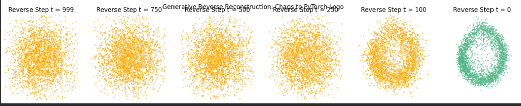
8. Scaling from 2D Points to Real-World Images (U-Net & Latent Diffusion)
Having mastered diffusion on 2D coordinates, how do these identical equations scale to high-resolution image synthesis?
8.1 2D Convolutional U-Net Architecture
For natural images $\mathbf{x} \in \mathbb{R}^{B \times C \times H \times W}$, the linear MLP is replaced with a 2D Convolutional U-Net backbone:
- Contracting (Encoder) Path: Successive residual convolutional blocks downsample spatial resolution via strided convolutions while increasing channel dimensionality (e.g., $64 \to 128 \to 256 \to 512$).
- Bottleneck with Self-Attention: Multi-Head Self-Attention layers compute global spatial dependencies at low spatial resolutions.
- Expanding (Decoder) Path: Successive transposed convolutions or nearest-neighbor upsamplings restore spatial dimensions, assisted by Skip Connections that concatenate high-resolution feature maps directly from encoder stages.
- Time & Text Conditioning: Timestep $t$ is projected via sinusoidal embeddings followed by MLPs and injected into every ResNet block via scale-and-shift Adaptive Group Normalization (
AdaGN):
$$ \text{AdaGN}(\mathbf{h}, t) = \mathbf{w}(t) \odot \left[\frac{\mathbf{h} - \mu}{\sigma}\right] + \mathbf{b}(t) $$
8.2 Latent Diffusion Models (LDMs / Stable Diffusion)
Direct pixel-space diffusion on $1024 \times 1024$ images requires astronomical computational resources because high-frequency pixel details require large tensor footprints.
Latent Diffusion Models (LDMs) solve this by decomposing generation into two stages:
- Perceptual Compression (Autoencoder): A pretrained VAE encoder compresses high-resolution images $\mathbf{x} \in \mathbb{R}^{3 \times 512 \times 512}$ by an 8x factor into a compact latent space $\mathbf{z} = \mathcal{E}(\mathbf{x}) \in \mathbb{R}^{4 \times 64 \times 64}$.
- Latent Space Diffusion: Diffusion operates entirely within the low-dimensional latent space $\mathbf{z}$.
- Cross-Attention Conditioning: Text prompts are encoded via CLIP / OpenCLIP text encoders and fused into the U-Net via Cross-Attention layers:
$$ \operatorname{Attention}(\mathbf{Q}, \mathbf{K}, \mathbf{V}) = \operatorname{softmax}\left(\frac{\mathbf{Q}\mathbf{K}^T}{\sqrt{d_k}}\right)\mathbf{V} $$
where queries $\mathbf{Q}$ are projected from spatial latent features and keys/values $(\mathbf{K}, \mathbf{V})$ are projected from token embeddings.
9. Exercises & Complete Analytical Solutions
Question 1: Fundamental Paradigm Differences
What are the core mathematical and operational differences between VAEs, GANs, and Diffusion Models for image synthesis?
Solution:
- VAEs: Maximize the Evidence Lower Bound (ELBO) using an encoder-decoder architecture. The latent space is explicitly regularized toward $\mathcal{N}(\mathbf{0}, \mathbf{I})$ via KL divergence. They offer fast, single-pass sampling and smooth latent interpolation, but produce blurry images due to pixel-wise MSE/Gaussian likelihood objectives.
- GANs: Optimize an implicit minimax zero-sum game between a Generator and Discriminator without computing likelihoods. They achieve sharp boundaries in a single forward pass, but suffer from mode collapse, training instability, and lack full distribution coverage.
- Diffusion Models: Formulate generation as reversing a forward Markov chain that systematically adds Gaussian noise. They optimize a convex, stable MSE loss ($\left\Vert \boldsymbol{\epsilon} - \boldsymbol{\epsilon}_\theta \right\Vert^2$) across all noise levels, achieving superior distribution diversity and sample fidelity without adversarial fragility. Their trade-off is inference latency due to iterative multi-step sampling.
Question 2: Point Coordinates vs. Image Pixels
How does adding noise to 2D coordinates $(p_0, p_1)$ mathematically compare to injecting noise into RGB image pixels $\mathbf{x} \in \mathbb{R}^{3 \times H \times W}$?
Solution: The mathematical operations are identical. In both cases, the data is represented as a tensor of continuous real-valued floats. The closed-form jump $\mathbf{x}_t = \sqrt{\bar{\alpha}_t}\mathbf{x}_0 + \sqrt{1 - \bar{\alpha}_t}\boldsymbol{\epsilon}$ operates element-wise across each tensor entry, whether the shape is $(N, 2)$ or $(B, 3, H, W)$. The only difference lies in the network architecture used to predict $\boldsymbol{\epsilon}$: 2D points use simple MLPs with sinusoidal coordinate embeddings, whereas images utilize 2D convolutional U-Nets with spatial receptive fields and self-attention.
Question 3: Noise Schedule Dynamics
Why must $\beta_t$ remain small ($\beta_1 = 10^{-4}$), and what happens if a constant schedule $\beta_t = 0.1$ is used instead?
Solution: The reverse step approximation $p_\theta(\mathbf{x}_{t-1} \mid \mathbf{x}_t) \approx q(\mathbf{x}_{t-1} \mid \mathbf{x}_t)$ mathematically assumes that each forward transition $q(\mathbf{x}_t \mid \mathbf{x}_{t-1})$ is a tiny perturbation such that the true reverse distribution remains Gaussian. If $\beta_t$ is excessively large (e.g., $0.1$ from step 1), the local Gaussian assumption breaks down, the model cannot distinguish intermediate structural scales, and reverse trajectory integration diverges into garbage artifacts.
Question 4: Accelerating Diffusion Sampling
Why is standard DDPM slow during inference, and how do modern frameworks (such as DDIM or SDXL-Lightning) overcome this limitation?
Solution: Standard DDPM requires $T \approx 1000$ sequential evaluations of the neural network to sample a single image because each step takes a microscopic reverse Markov jump. Modern techniques accelerate this:
- DDIM (Denoising Diffusion Implicit Models): Replaces the stochastic Markov chain with a non-Markovian deterministic ODE solver that skips intermediate timesteps, generating high-quality samples in 20–50 steps.
- Flow Matching & Consistency Models (SDXL-Lightning / FLUX): Train models to map any point along the trajectory directly to the clean distribution or integrate continuous-time velocity fields, reducing sampling to 1–4 inference steps.
10. Chapter Summary & Key Takeaways
- Generative Vision Goal: Image synthesis models the true underlying data distribution $p_{\text{data}}(\mathbf{x})$ to sample novel, coherent visual scenes.
- Predecessor Architectures: VAEs maximize the ELBO via latent autoencoding (yielding stable but blurry images); GANs pit generator against discriminator in a minimax game (producing sharp images vulnerable to mode collapse).
- Physical Analogy: Diffusion models reverse a physical noising process, progressively destroying data structure into standard Gaussian entropy ($\mathcal{N}(\mathbf{0}, \mathbf{I})$) and learning to reconstruct it step by step.
- Forward Closed-Form Expression: Using $\alpha_t = 1 - \beta_t$ and cumulative product $\bar{\alpha}_t = \prod_{s=1}^t \alpha_s$, any noisy state $\mathbf{x}_t$ is sampled in $\mathcal{O}(1)$ time via: $$ \mathbf{x}_t = \sqrt{\bar{\alpha}_t}\mathbf{x}_0 + \sqrt{1 - \bar{\alpha}_t}\boldsymbol{\epsilon} $$
- Training Objective ($L_{\text{simple}}$): The neural network $\boldsymbol{\epsilon}_\theta(\mathbf{x}_t, t)$ is trained via unweighted Mean Squared Error (MSE) to predict the injected noise vector: $$ L_{\text{simple}}(\theta) = \mathbb{E}_{t, \mathbf{x}_0, \boldsymbol{\epsilon}}\left[ \left\Vert \boldsymbol{\epsilon} - \boldsymbol{\epsilon}_\theta(\mathbf{x}_t, t) \right\Vert^2 \right] $$
- Sinusoidal Embeddings: Multi-scale trigonometric embeddings inject critical continuous time and coordinate parameters into linear layers and ResNet blocks.
- Reverse Sampling: Ancestral sampling iteratively denoises pure Gaussian noise from $t=T$ to $t=0$, reconstructing crisp geometric and pixel structures from chaos.
- Industry Scale: Foundation models (DALL-E, Stable Diffusion, SDXL) leverage 2D Convolutional U-Nets, Latent Autoencoders (LDMs), and Cross-Attention to generate photorealistic imagery from natural language prompts.
Using PyTorch to Fight Cancer
- 1. The Clinical Problem: Lung Cancer & The LUNA Grand Challenge
- 2. What Is a CT Scan, Exactly?
- 3. 3D Volumetric Representation & Cartesian Space
- 4. The Project Architecture: An End-to-End Cancer Detector
- 5. What Is a Nodule? Anatomy & Morphology
- 6. The LUNA Grand Challenge Dataset Anatomy
- 7. Coordinate Geometry: From Array Indices to Millimeter Space
- 8. Micro-Modular Implementation Walkthrough
- 9. Summary & Looking Ahead to Chapter 12
1. The Clinical Problem: Lung Cancer & The LUNA Grand Challenge
Lung cancer is the leading cause of cancer-related mortality worldwide, accounting for roughly 1.8 million deaths annually. The clinical tragedy of lung cancer lies in its asymptomatic progression: early-stage pulmonary nodules rarely cause discomfort, meaning the majority of patients are diagnosed only after malignant cells have metastasized to regional lymph nodes or distant organs, dropping five-year survival rates precipitously from over 60% down to less than 10%.
flowchart TD
subgraph ClinicalProgression ["Clinical Disease Progression vs Diagnostic Window"]
NoduleEarly["Stage I: Solitary Pulmonary Nodule (1-2 cm, Asymptomatic)"] --> Resection["Surgical Resection / Curative Ablation (>60% 5-Year Survival)"]
NoduleEarly -. "Undetected / Late Screening" .-> NoduleLate["Stage IV: Metastatic Carcinoma (Systemic Spread)"]
NoduleLate --> Palliative["Palliative Systemic Therapy (<10% 5-Year Survival)"]
end
style ClinicalProgression fill:#1a1a2e,stroke:#4cc9f0,stroke-width:2px,color:#fff
style Resection fill:#1a3a2a,stroke:#52b788,stroke-width:2px,color:#fff
style Palliative fill:#3a1a1a,stroke:#e63946,stroke-width:2px,color:#fff
When low-dose helical Computerized Tomography (CT) screening was validated by the National Lung Screening Trial (NLST), evidence confirmed that proactive screening reduced lung cancer mortality by 20%. However, this diagnostic advantage introduced a severe radiologist bottleneck:
- Volumetric Information Overload: A modern high-resolution thoracic CT scan comprises hundreds of axial slices per patient, producing millions of individual voxels that a human expert must visually inspect.
- False-Positive Fatigue: The overwhelming majority (frequently $>95%$) of tiny candidate tissue clusters identified during initial screening are benign granulomas, intrapulmonary lymph nodes, or apical scars.
- Inter-Reader Variability: Subtle visual cues differentiating an indolent benign hamartoma from an invasive adenocarcinoma (such as ground-glass opacity, lobulation, or coronal spiculation) often lead to discordant clinical opinions.
To catalyze automated computer-aided detection (CAD) systems, the academic and clinical research community assembled the LUng Nodule Analysis (LUNA) Grand Challenge (built upon the public LIDC-IDRI database). LUNA provides standardized, expert-annotated thoracic CT volumes alongside rigid evaluation metrics (such as the Free-Response Receiver Operating Characteristic, FROC), establishing the definitive benchmark for computer vision systems operating on volumetric medical imagery.
2. What Is a CT Scan, Exactly?
2.1 The Physics of X-Ray Computed Tomography
Unlike standard photography—which captures photons reflected off the opaque outer surface of objects across visible wavelengths—Computed Tomography measures the attenuation of high-energy electromagnetic radiation (X-rays, photon energy roughly $20\text{ to }140\text{ keV}$) as it penetrates through heterogeneous biological matter.
When a narrow beam of monoenergetic X-ray photons with initial incident intensity $I_0$ travels a path length $x$ through a uniform medium with linear attenuation coefficient $\mu$, photon absorption and Compton scattering diminish beam intensity according to the classical Beer-Lambert Law:
$$ I = I_0 , e^{-\mu x} $$
In the human body, tissues possess continuously varying elemental compositions and physical densities $\rho(\mathbf{x})$, yielding a spatially continuous attenuation field $\mu(x, y, z)$. As the X-ray tube and detector array rotate synchronously around the patient’s gantry, the detector records line integrals of attenuation (the Radon Transform):
$$ p(\theta, s) = \int_{-\infty}^{\infty} \int_{-\infty}^{\infty} \mu(x, y) , \delta(x \cos\theta + y \sin\theta - s) , dx , dy $$
Applying the Fourier Slice Theorem and filtered backprojection (FBP) or iterative algebraic reconstruction algorithms, tomographic reconstruction algorithms reconstruct the internal 2D cross-sectional slice $\mu(x, y)$ from hundreds of 1D angular projection profiles.
2.2 The Hounsfield Unit (HU) Radiodensity Scale
Raw attenuation coefficients $\mu$ depend heavily on the X-ray tube peak kilovoltage ($kVp$) and beam hardening artifacts. To standardize readings across scanner manufacturers, imaging protocols, and hospital sites, Sir Godfrey Hounsfield established a calibrated, unitless radiodensity metric known as the Hounsfield Unit (HU).
The HU transformation maps physical attenuation linearly relative to the attenuation of distilled water ($\mu_{\text{water}}$) and ambient air ($\mu_{\text{air}} \approx 0$) under standard temperature and pressure:
$$ \text{HU} = 1000 \times \frac{\mu - \mu_{\text{water}}}{\mu_{\text{water}} - \mu_{\text{air}}} $$
By international convention and physical definition:
- Air: $-1000\text{ HU}$ (minimal photon attenuation)
- Lung Parenchyma (aerated alveoli): $-900\text{ to }-500\text{ HU}$
- Fat (Adipose Tissue): $-120\text{ to }-90\text{ HU}$
- Distilled Water: $0\text{ HU}$ (the baseline reference)
- Blood & Muscle / Soft Tissue: $+20\text{ to }+50\text{ HU}$
- Pulmonary Nodules / Solid Tumors: $+30\text{ to }+100\text{ HU}$
- Dense Cortical Bone: $+500\text{ to }+1500\text{ HU}$
- Metal Implants (Dental fills, surgical clips): $+3000\text{ HU}$ and above
flowchart TD
subgraph HUScale ["Hounsfield Unit (HU) Radiodensity Spectrum"]
Air["Air (-1000 HU)"] --> Lung["Lung Tissue (-900 to -500 HU)"]
Lung --> Fat["Adipose Tissue (-100 HU)"]
Fat --> Water["Water Reference (0 HU)"]
Water --> Soft["Soft Tissue / Blood (+30 to +60 HU)"]
Soft --> Nodule["Solid Tumors / Nodules (+50 to +100 HU)"]
Nodule --> Bone["Cortical Bone (+700 to +1500 HU)"]
end
style Air fill:#0f172a,stroke:#38bdf8,color:#fff
style Lung fill:#1e293b,stroke:#0ea5e9,color:#fff
style Water fill:#0284c7,stroke:#38bdf8,color:#fff
style Soft fill:#1e3a5f,stroke:#60a5fa,color:#fff
style Nodule fill:#b91c1c,stroke:#f87171,color:#fff
style Bone fill:#475569,stroke:#cbd5e1,color:#fff
Because human visual perception cannot resolve the full dynamic range of roughly 4000 distinct Hounsfield values on an 8-bit display ($256$ grayscale levels), medical imaging software applies Windowing (Window Width $W$ and Window Level $L$):
$$ I_{\text{display}} = \text{clip}\left( \frac{\text{HU} - (L - W/2)}{W} \times 255, , 0, , 255 \right) $$
For pulmonary nodule evaluation, radiologists select a Lung Window ($W = 1500, L = -600$), which expands aerated lung structures across full contrast while clipping dense mediastinal and bone structures to pure white ($255$).
3. 3D Volumetric Representation & Cartesian Space
A standard photographic image is a 2D matrix of square pixels indexed by row and column $(r, c)$. In contrast, a modern thoracic CT acquisition yields a 3D volumetric array of rectangular cuboids known as voxels (volume elements).
3.1 Non-Isotropic Voxel Geometry
A critical difference between standard computer vision inputs and medical CT arrays is that CT voxels are frequently non-isotropic (the spatial resolution is not equal along all three spatial axes):
- In-Plane Resolution ($\Delta x, \Delta y$): Typically $0.6\text{ to }0.8\text{ mm}$ per pixel across a $512 \times 512$ axial slice grid.
- Slice Thickness ($\Delta z$): The distance between consecutive gantry acquisitions along the patient’s cranio-caudal axis. In high-resolution screening protocols, $\Delta z$ ranges from $1.0\text{ mm}$ to $2.5\text{ mm}$, but older or routine clinical scans often possess slice thicknesses of $5.0\text{ mm}$.
If a deep neural network processes raw voxel arrays without accounting for voxel spacing $(\Delta z, \Delta y, \Delta x)$, a spherical $10\text{ mm}$ nodule will appear severely compressed or elongated along the $Z$-axis, distorting morphological features and degrading convolutional filter responses.
4. The Project Architecture: An End-to-End Cancer Detector
Directly feeding a full $512 \times 512 \times 400$ thoracic CT volume into a 3D convolutional neural network is computationally intractable. A single patient volume contains:
$$ 512 \times 512 \times 400 = 104,857,600 \text{ voxels} $$
At 32-bit floating point precision ($4\text{ bytes}$ per voxel), storing one volume in memory requires over $419\text{ MB}$ of VRAM. Retaining intermediate feature activations during backpropagation for modern deep 3D architectures (such as 3D ResNets) quickly exceeds the physical memory limits of even flagship datacenter GPUs ($80\text{ GB}$).
Furthermore, a typical solitary pulmonary nodule spans roughly $10\text{ to }15\text{ voxels}$ in diameter, occupying a microscopic volume of roughly $1000\text{ voxels}$—less than 0.001% of the total scan volume. Designing a single model to find this tiny needle in a $105\text{ million}$ voxel haystack induces catastrophic class imbalance.
To resolve this challenge, the standard industry and literature approach decomposes the cancer detection task into an elegant three-stage divide-and-conquer pipeline:
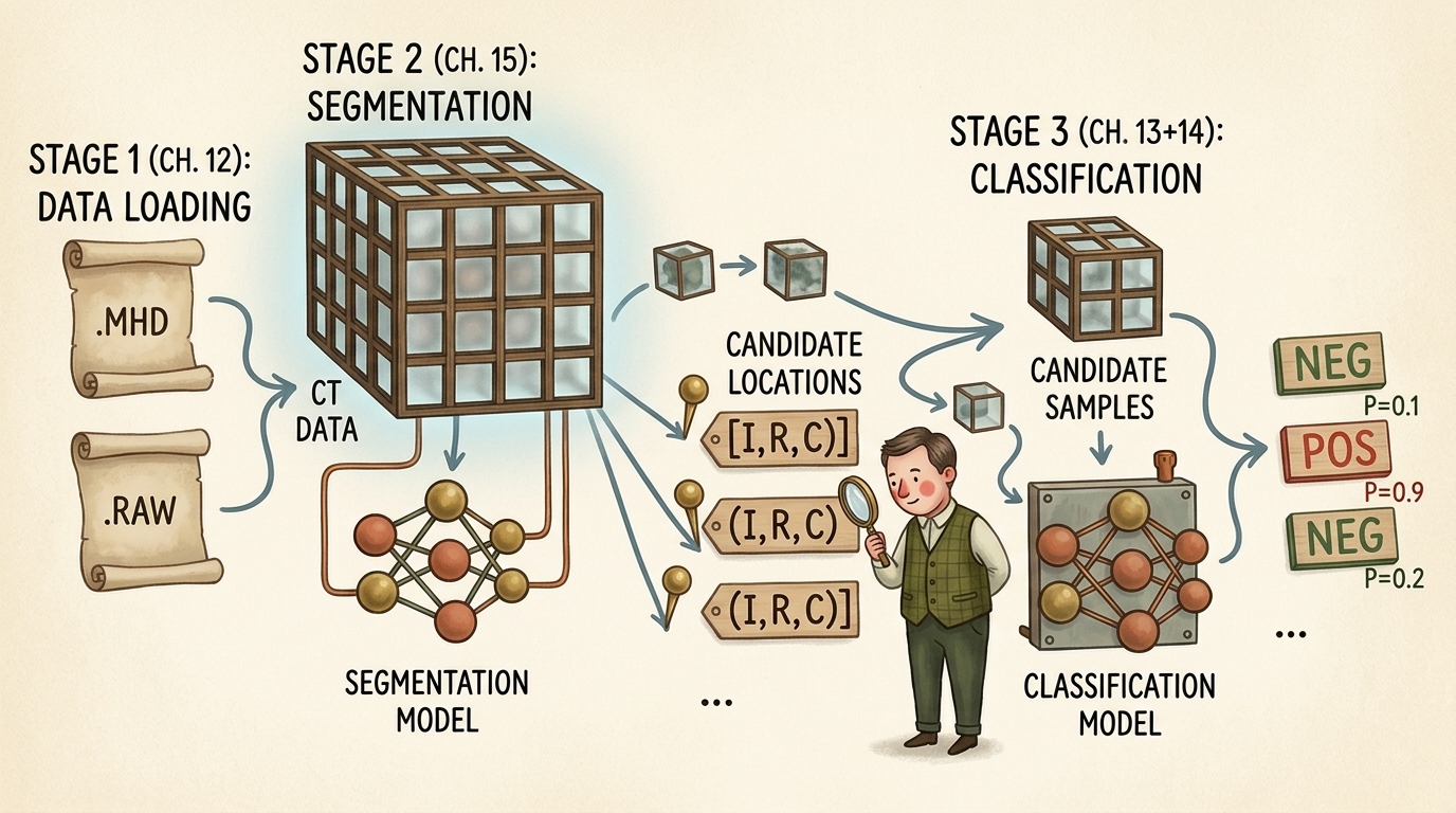
flowchart TD
subgraph Stage1 ["Stage 1: Raw Data Ingestion & Geometry (Chapter 12)"]
RawFiles[".MHD Header & .RAW Binary Scan"] --> SimpleITK["SimpleITK Parsing & Voxel Decompression"]
SimpleITK --> CoordTransform["Coordinate Normalization (IRC to World XYZ)"]
CoordTransform --> VolCT["3D CT Volume (Hounsfield Units)"]
end
subgraph Stage2 ["Stage 2: Candidate Generation via Segmentation (Chapter 15)"]
VolCT --> SegNet["2D/3D Semantic Segmentation (U-Net)"]
SegNet --> ComponentAnalysis["Connected Component Labeling & Grouping"]
ComponentAnalysis --> CandidateList["Candidate Nodule Locations [(Index, Row, Col), ...]"]
end
subgraph Stage3 ["Stage 3: False Positive Reduction via Classification (Chapters 13-14)"]
CandidateList --> CropEngine["Subvolume Cropper (e.g. 32x48x48 Voxel Patches)"]
VolCT --> CropEngine
CropEngine --> ClassNet["3D Deep Convolutional Classifier (3D ResNet)"]
ClassNet --> Decision["Final Malignancy Probabilities: P(Malignant) in [0.0, 1.0]"]
end
Stage1 --> Stage2
Stage2 --> Stage3
style Stage1 fill:#1e293b,stroke:#38bdf8,stroke-width:2px,color:#fff
style Stage2 fill:#14342b,stroke:#52b788,stroke-width:2px,color:#fff
style Stage3 fill:#2d1b36,stroke:#c084fc,stroke-width:2px,color:#fff
Breakdown of the Pipeline Stages:
- Stage 1 (Data Ingestion & Coordinate Geometry — Chapter 12):
Parse raw medical formats (
.mhd/.raw), extract affine orientation and spacing matrices, normalize voxel intensities to standardized Hounsfield Units, and map coordinates between discrete array storage and millimeter patient space. - Stage 2 (Candidate Generation via Segmentation — Chapter 15): Deploy a fast semantic segmentation network (such as a 2D or 3D U-Net) to identify all high-density spherical candidates inside lung parenchyma. This stage is tuned for near-100% sensitivity (recall): we accept thousands of false alarms (blood vessel bifurcations, bronchial wall thickenings) to ensure zero true malignant nodules are overlooked.
- Stage 3 (False Positive Reduction & Classification — Chapters 13 & 14): Extract compact 3D bounding cubes (e.g., $32 \times 48 \times 48\text{ voxels}$) centered precisely at each candidate location. A specialized 3D Convolutional Neural Network evaluates fine-grained volumetric texture, boundary spiculation, internal calcification patterns, and surrounding vascular attachments to filter out benign structures and assign calibrated malignancy scores.
5. What Is a Nodule? Anatomy & Morphology
Clinically, a pulmonary nodule is defined as a well-circumscribed, roughly spherical radiographic opacity with a diameter of up to $30\text{ mm}$ surrounded by aerated lung tissue. Lesions larger than $30\text{ mm}$ are classified as pulmonary masses and carry a dramatically higher statistical probability of active malignancy.
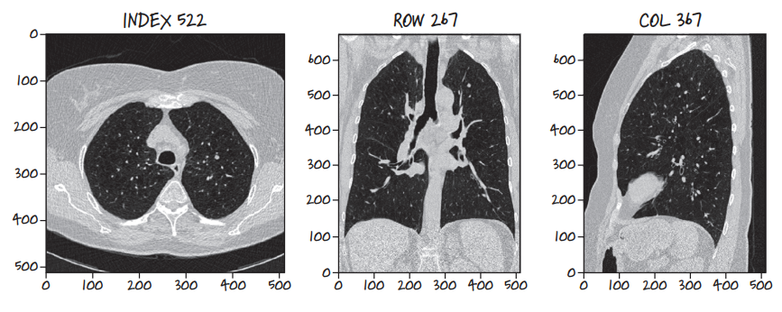
5.1 The Three Orthogonal Viewing Planes
Because a CT scan is a contiguous 3D volume, it can be resliced along any arbitrary geometric plane. Three anatomical orthogonal planes form the foundation of clinical radiology:
- Axial (Transverse) Plane: Slices perpendicular to the spine, looking upward from the patient’s feet toward the head ($XY$-plane at constant $Z$, indexed as
Index). - Coronal (Frontal) Plane: Slices slicing through the body from chest to back ($XZ$-plane at constant $Y$, indexed as
Row). - Sagittal (Lateral) Plane: Slices dividing the patient into left and right halves ($YZ$-plane at constant $X$, indexed as
Col).
Examining lesions across all three orthogonal projections is mandatory: a tubular blood vessel running along the axial plane may appear circular like a nodule on a single 2D slice, but coronal and sagittal views immediately expose its elongated, branching vascular geometry.
5.2 Sequential Multi-Slice Spherical Expansion
Because nodules are 3D spherical or ellipsoidal geometries, slicing sequentially through the volume reveals a distinct cross-sectional profile: the nodule appears as a faint point, grows symmetrically to its maximum equatorial diameter, and contracts until fading out of view.
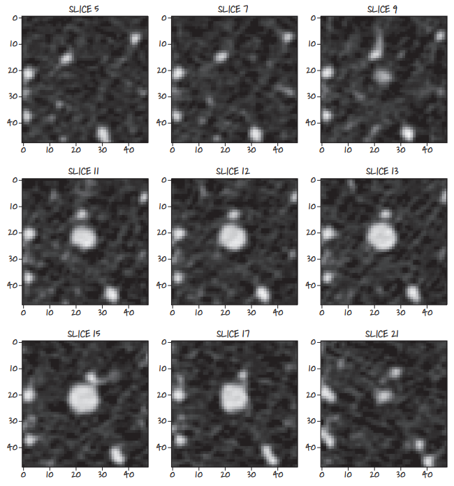
5.3 Benign vs Malignant Pathological Indicators
Radiologists evaluate several subtle textural and structural features to differentiate benign lesions from malignant carcinomas:
- Spiculation: Sharp, needle-like radiating strands extending outward from the lesion margin into aerated lung parenchyma. Strongest clinical indicator of invasive malignancy.
- Lobulation: Scalloped, uneven contour lobes reflecting uneven clonal growth rates of malignant cells.
- Calcification Patterns: Dense central, concentric, or “popcorn” calcification patterns typically signify benign granulomas or hamartomas. Eccentric, stippled calcifications suggest malignancy.
- Ground-Glass Opacity (GGO): Hazy attenuation that does not obscure underlying bronchial structures and blood vessels, frequently associated with early adenocarcinoma in situ.
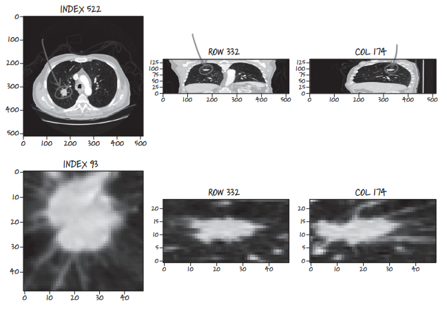
6. The LUNA Grand Challenge Dataset Anatomy
The LUNA16 challenge dataset provides 888 thoracic CT scans categorized into 10 subsets (subset0 through subset9).
6.1 MetaImage Format: .mhd Headers & .raw Binary Buffers
Rather than storing hundreds of separate DICOM files per patient, LUNA encodes each volume as a paired MetaImage dataset:
.mhd(MetaImage Header): A clean plain-text ASCII header file detailing dimensional metadata:DimSize = 512 512 360(dimensions along X, Y, and Z)ElementType = MET_SHORT(signed 16-bit integer,int16)ElementSpacing = 0.703125 0.703125 1.25(physical voxel size in mm)Offset = -175.2 -175.2 -312.5(origin of voxel[0, 0, 0]in patient mm space)TransformMatrix = 1 0 0 0 1 0 0 0 1(direction cosine orientation)ElementDataFile = 1.3.6.1.4.1.14519.5.2.1.6279.6001.100225287222365630678668347788.raw
.raw(Binary Image Buffer): Uncompressed, contiguous 1D binary buffer of signed 16-bit integers storing all voxels sequentially in row-major order.
6.2 Annotation Schema: Ground Truth vs Candidate Lists
LUNA provides two distinct CSV annotation files:
annotations.csv: Ground truth pulmonary nodules consensus-annotated by at least 3 out of 4 expert thoracic radiologists.seriesuid: Unique patient scan identifier string.coordX, coordY, coordZ: Exact spatial centroid of the nodule in millimeter patient space.diameter_mm: Equivalent spherical diameter in millimeters.
candidates.csv: A comprehensive list of approximately 750,000 candidate locations generated by classical candidate filtering algorithms.seriesuid, coordX, coordY, coordZ: Candidate centroid location.class: Binary label (0for benign non-nodule/false alarm,1for true validated nodule). True positives account for roughly 1,351 out of 750,000 entries (a severe 1:550 imbalance).
7. Coordinate Geometry: From Array Indices to Millimeter Space
A frequent source of catastrophic bugs in medical deep learning pipelines is coordinate system confusion. Array indices in memory and physical patient locations in space do not share origin, orientation, or units.
flowchart TD
subgraph CoordinateDomains ["Coordinate Spaces in Medical Imaging"]
IRC["Array Space (Storage): Index, Row, Column (i, r, c) in Z, Y, X"] --> Scaled["Voxel Space Scaled by Spacing: (i*dz, r*dy, c*dx)"]
Scaled --> Affine["Rotation by Direction Matrix D + Origin Translation O"]
Affine --> World["Physical Patient Space: World Coordinates (X, Y, Z) in mm"]
end
style CoordinateDomains fill:#1a1a2e,stroke:#4cc9f0,stroke-width:2px,color:#fff
style IRC fill:#1e293b,stroke:#0ea5e9,color:#fff
style World fill:#14342b,stroke:#52b788,color:#fff
7.1 Coordinate Definitions
- Array Space ($I, R, C$): Discrete 0-based integer indices indexing the 3D tensor buffer:
- $I$ (
Index): Slice along $Z$-axis (axial gantry position). - $R$ (
Row): Row index along $Y$-axis (vertical dimension of axial image). - $C$ (
Column): Column index along $X$-axis (horizontal dimension of axial image).
- $I$ (
- Physical World Space ($X, Y, Z$): Continuous floating-point coordinates measured in millimeters relative to the scanner’s physical origin isocenter:
- $X$: Left $(-)$ to Right $(+)$ across the patient’s body.
- $Y$: Anterior / front $(-)$ to Posterior / back $(+)$.
- $Z$: Inferior / feet $(-)$ to Superior / head $(+)$.
7.2 The Transformation Formulas
Given origin $\mathbf{O} = (O_x, O_y, O_z)$, voxel spacing $\mathbf{s} = (s_x, s_y, s_z)$, and direction matrix $\mathbf{D} \in \mathbb{R}^{3 \times 3}$, mapping an array index $\mathbf{v}_{\text{irc}} = (i, r, c)^T$ (note the reverse order to $(c, r, i) = (x, y, z)$) to patient world coordinates $\mathbf{x}_{\text{xyz}} = (x, y, z)^T$ follows the affine transformation:
$$ \mathbf{x}_{\text{xyz}} = \mathbf{O} + \mathbf{D} \begin{bmatrix} c \cdot s_x \ r \cdot s_y \ i \cdot s_z \end{bmatrix} $$
Assuming an identity orientation matrix $\mathbf{D} = \mathbf{I}_3$ (standard for LUNA scans), the inverse mapping from millimeter patient space to discrete array indices is computed as:
$$ c = \text{round}\left( \frac{x - O_x}{s_x} \right), \quad r = \text{round}\left( \frac{y - O_y}{s_y} \right), \quad i = \text{round}\left( \frac{z - O_z}{s_z} \right) $$
8. Micro-Modular Implementation Walkthrough
Let us implement the core data structures and geometric transformations using PyTorch and NumPy.
Step 1: Defining Coordinate Data Structures
We construct lightweight named tuples to prevent inversion bugs between $(X, Y, Z)$ and $(I, R, C)$ coordinate orders:
from collections import namedtuple
import numpy as np
import torch
# Immutable, strongly-typed representations of our coordinate spaces
IrcTuple = namedtuple('IrcTuple', ['index', 'row', 'col'])
XyzTuple = namedtuple('XyzTuple', ['x', 'y', 'z'])
Step 2: Bidirectional Coordinate Transformation Functions
Next, we define mathematical transform functions mapping between physical millimeter coordinates and discrete voxel array indices:
def xyz2irc(coord_xyz: XyzTuple, origin_xyz: XyzTuple, vx_per_mm_xyz: XyzTuple, direction_mat: np.ndarray = None) -> IrcTuple:
"""
Transforms continuous physical world millimeter coordinates (X, Y, Z)
into discrete 3D array indices (Index, Row, Column).
"""
# Offset from physical origin
diff_x = coord_xyz.x - origin_xyz.x
diff_y = coord_xyz.y - origin_xyz.y
diff_z = coord_xyz.z - origin_xyz.z
# Scale by voxels per millimeter (1 / spacing)
col = int(round(diff_x * vx_per_mm_xyz.x))
row = int(round(diff_y * vx_per_mm_xyz.y))
index = int(round(diff_z * vx_per_mm_xyz.z))
return IrcTuple(index=index, row=row, col=col)
def irc2xyz(coord_irc: IrcTuple, origin_xyz: XyzTuple, spacing_xyz: XyzTuple, direction_mat: np.ndarray = None) -> XyzTuple:
"""
Transforms discrete 3D array indices (Index, Row, Column)
into continuous physical world millimeter coordinates (X, Y, Z).
"""
x = coord_irc.col * spacing_xyz.x + origin_xyz.x
y = coord_irc.row * spacing_xyz.y + origin_xyz.y
z = coord_irc.index * spacing_xyz.z + origin_xyz.z
return XyzTuple(x=x, y=y, z=z)
Step 3: Hounsfield Unit Windowing and Tensor Normalization
To prepare raw CT volumes for neural network ingestion, we construct a windowing function that clamps values to the standard clinical lung window $[-1000\text{ HU}, +400\text{ HU}]$ and normalizes intensities to the $[0.0, 1.0]$ range:
def apply_lung_window(ct_tensor: torch.Tensor, min_hu: float = -1000.0, max_hu: float = 400.0) -> torch.Tensor:
"""
Clamps raw CT Hounsfield Units to the standard lung window range
and normalizes linearly to [0.0, 1.0].
Args:
ct_tensor (torch.Tensor): Raw voxel tensor in Hounsfield Units.
min_hu (float): Lower HU bound (pure air = -1000).
max_hu (float): Upper HU bound (mediastinum/bone = +400).
Returns:
torch.Tensor: Normalized floating-point tensor in [0.0, 1.0].
"""
clamped = torch.clamp(ct_tensor, min=min_hu, max=max_hu)
normalized = (clamped - min_hu) / (max_hu - min_hu)
return normalized
Step 4: Extracting Fixed 3D Candidate Subvolumes for PyTorch
Finally, given a candidate coordinate $(I, R, C)$, we extract a fixed cubic bounding patch (e.g., $32 \times 48 \times 48\text{ voxels}$) suitable for direct feeding into a 3D PyTorch convolution layer:
def extract_candidate_subvolume(
ct_volume: torch.Tensor,
center_irc: IrcTuple,
crop_shape_irc: tuple = (32, 48, 48)
) -> torch.Tensor:
"""
Extracts a 3D subvolume tensor centered at center_irc, padding with air (-1000 HU)
if the crop boundary exceeds the scan volume dimensions.
Returns:
torch.Tensor: Tensor with shape (1, 1, Depth, Height, Width) ready for 3D CNNs.
"""
half_i = crop_shape_irc[0] // 2
half_r = crop_shape_irc[1] // 2
half_c = crop_shape_irc[2] // 2
pad_i = max(0, half_i - center_irc.index)
pad_r = max(0, half_r - center_irc.row)
pad_c = max(0, half_c - center_irc.col)
start_i = max(0, center_irc.index - half_i)
end_i = min(ct_volume.shape[0], center_irc.index + half_i)
start_r = max(0, center_irc.row - half_r)
end_r = min(ct_volume.shape[1], center_irc.row + half_r)
start_c = max(0, center_irc.col - half_c)
end_c = min(ct_volume.shape[2], center_irc.col + half_c)
subvolume = ct_volume[start_i:end_i, start_r:end_r, start_c:end_c]
# Pad to exact crop_shape if near scan boundaries
subvolume_padded = torch.nn.functional.pad(
subvolume,
(
max(0, half_c - (center_irc.col - start_c)),
max(0, half_c - (end_c - center_irc.col)),
max(0, half_r - (center_irc.row - start_r)),
max(0, half_r - (end_r - center_irc.row)),
max(0, half_i - (center_irc.index - start_i)),
max(0, half_i - (end_i - center_irc.index)),
),
value=-1000.0 # Pad with air HU
)
# Reshape to (Batch, Channel, Depth, Height, Width)
return subvolume_padded.unsqueeze(0).unsqueeze(0)
9. Summary & Looking Ahead to Chapter 12
In this chapter, we established the foundational principles of medical computerized tomography and the end-to-end lung cancer detection problem:
- CT Physics & Radiometry: CT measures physical attenuation of X-rays, standardized into unitless Hounsfield Units (HU) relative to air ($-1000$) and water ($0$).
- Volumetric Geometry: Thoracic CT scans are 3D arrays of non-isotropic voxels, requiring explicit conversion between discrete array indexing $(I, R, C)$ and continuous millimeter patient space $(X, Y, Z)$.
- The Divide-and-Conquer Architecture: Due to extreme memory constraints ($>100\text{ million voxels}$) and severe class imbalance ($1:550$), the system splits the task into Data Ingestion (Ch. 12), Candidate Segmentation (Ch. 15), and 3D Classification (Ch. 13–14).
In Chapter 12: Combining Data Sources into a Unified Dataset, we will build a high-throughput, multi-threaded PyTorch Dataset that reads raw .mhd and .raw files using SimpleITK, caches parsed volumes to high-speed storage, and dynamically streams balanced candidate batches into our training loops.
Combining Data Sources into a Unified Dataset
- 1. The Data Ingestion Bottleneck in 3D Medical Deep Learning
- 2. Master Data Pipeline Architecture
- 3. Parsing LUNA Annotation & Candidate Records
- 4. Ingesting Raw CT Scans & The MetaImage Format
- 5. Spatial Coordinate Systems & Afin Transformations
- 6. The Three Orthogonal Anatomical Planes
- 7. Extracting 3D Volumetric Candidate Crops
- 8. High-Performance Caching & PyTorch Dataset Architecture
- 9. Conclusion & Next Steps
1. The Data Ingestion Bottleneck in 3D Medical Deep Learning
In standard computer vision workflows—such as classification on ImageNet or object detection on COCO—datasets consist of isolated 2D PNG or JPEG image files where pixel indices directly correspond to image coordinates. Medical imaging, and high-resolution thoracic Computerized Tomography (CT) in particular, shatters this simplicity across several fundamental architectural dimensions:
- Massive Volumetric Scale: A single thoracic CT scan comprises a volumetric 3D lattice consisting of hundreds of sequential 2D slices (typically $512 \times 512$ voxels across 150–500 axial planes), consuming $50\text{ MB to }200\text{ MB}$ of raw uncompressed memory per patient.
- Separation of Physical Space and Digital Arrays: Physical structures in human anatomy are measured in absolute millimeters ($X, Y, Z$), whereas tensors are indexed by discrete integer matrix subscripts ($[I, R, C]$). Because scanners operate with varying slice thicknesses and field-of-view settings, the spatial relationship between physical millimeters and discrete voxels differs across patients.
- Severe Class Imbalance: In the LUNA (LUng Nodule Analysis) Grand Challenge dataset, expert thoracic radiologists annotated approximately $1{,}351$ genuine malignant/benign nodules across $888$ patient scans, while automated classical candidate extractors flagged over $550{,}000$ suspicious tissue locations. Genuine nodules constitute less than $0.25%$ of all candidate samples.
- Data Leakage Risks: Multiple candidate tissue patches frequently belong to the same patient volume. Randomly shuffling candidates across train and validation splits would allow slices from the same anatomical volume into both partitions, invalidating validation accuracy.
This module establishes Step 1: Data Loading & Preprocessing of the end-to-end lung cancer detection system, transforming raw heterogeneous CT disk files and CSV annotation catalogs into a memory-efficient, cached PyTorch Dataset that yields uniform 3D tensor patches.
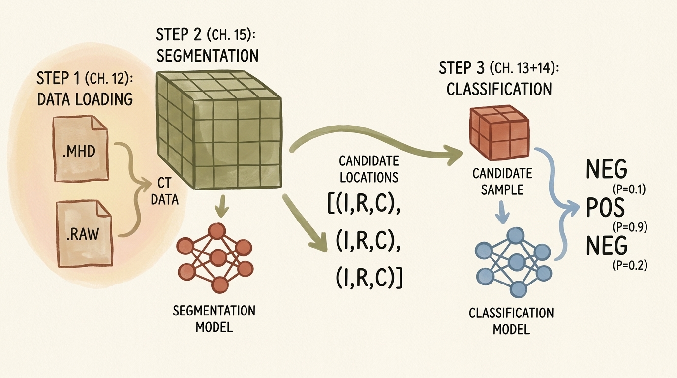
flowchart TD
subgraph StorageLayer ["Disk Storage Layer"]
direction TB
subgraph CTFiles ["Volumetric CT Scans (.mhd / .raw)"]
direction LR
MHD[".mhd Header Files<br/>(Origin, Spacing, Direction)"]
RAW[".raw Binary Files<br/>(Little-Endian Int16 HU)"]
end
subgraph CSVFiles ["Tabular Catalogs (.csv)"]
direction LR
CSVAnn["annotations.csv<br/>(True Nodules: Series, XYZ, Diam)"]
CSVCand["candidates.csv<br/>(All Candidates: Series, XYZ, Class)"]
end
CTFiles --> CSVFiles
end
subgraph ParsingEngine ["Data Synthesis & Coordinate Resolution"]
direction TB
AnnotParse["Parse & Merge Annotations<br/>by series_uid & Spatial Distance"]
SITKLoad["SimpleITK Volumetric Ingestion:<br/>Extract Origin, Spacing, Voxel Array"]
AffineCoord["Affine Transformation:<br/>Patient Space (mm) ➔ Voxel Space (IRC)"]
AnnotParse --> SITKLoad --> AffineCoord
end
subgraph MemoryOptimization ["Patch Extraction & Tiered Caching"]
direction TB
PatchCrop["Extract 3D Sub-Volume Patch<br/>(32 x 32 x 32 Voxels)"]
HUClamp["Hounsfield Clamping:<br/>[-1000 HU, +1000 HU] ➔ Float32 Normalization"]
TierCache["Tiered Caching:<br/>In-Memory (lru_cache) + Disk Persistence (diskcache)"]
PatchCrop --> HUClamp --> TierCache
end
subgraph DatasetInterface ["PyTorch Dataset Abstraction (LunaDataset)"]
direction TB
SampleTuple["__getitem__ Output:<br/>(Tensor[1, 32, 32, 32], Label[0/1], series_uid, Center_IRC)"]
GroupSplit["Grouped Split:<br/>10-Fold Series UID Cross-Validation (Zero Leakage)"]
SampleTuple --> GroupSplit
end
StorageLayer --> ParsingEngine
ParsingEngine --> MemoryOptimization
MemoryOptimization --> DatasetInterface
style StorageLayer fill:#1a1a2e,stroke:#4cc9f0,stroke-width:2px,color:#fff
style CTFiles fill:#16213e,stroke:#4cc9f0,stroke-width:1px,color:#fff
style CSVFiles fill:#16213e,stroke:#4cc9f0,stroke-width:1px,color:#fff
style ParsingEngine fill:#1a3a2a,stroke:#52b788,stroke-width:2px,color:#fff
style MemoryOptimization fill:#2a1a3a,stroke:#bd53ed,stroke-width:2px,color:#fff
style DatasetInterface fill:#3a2a1a,stroke:#ffaa00,stroke-width:2px,color:#fff
2. Master Data Pipeline Architecture
The unified dataset pipeline bridges two distinct data streams:
- Volumetric Medical Imaging Stream: Large volumetric CT scans stored in the MetaImage format (
.mhd+.raw). - Tabular Annotation Stream: Comma-separated value (CSV) files specifying candidate coordinates and clinical labels.
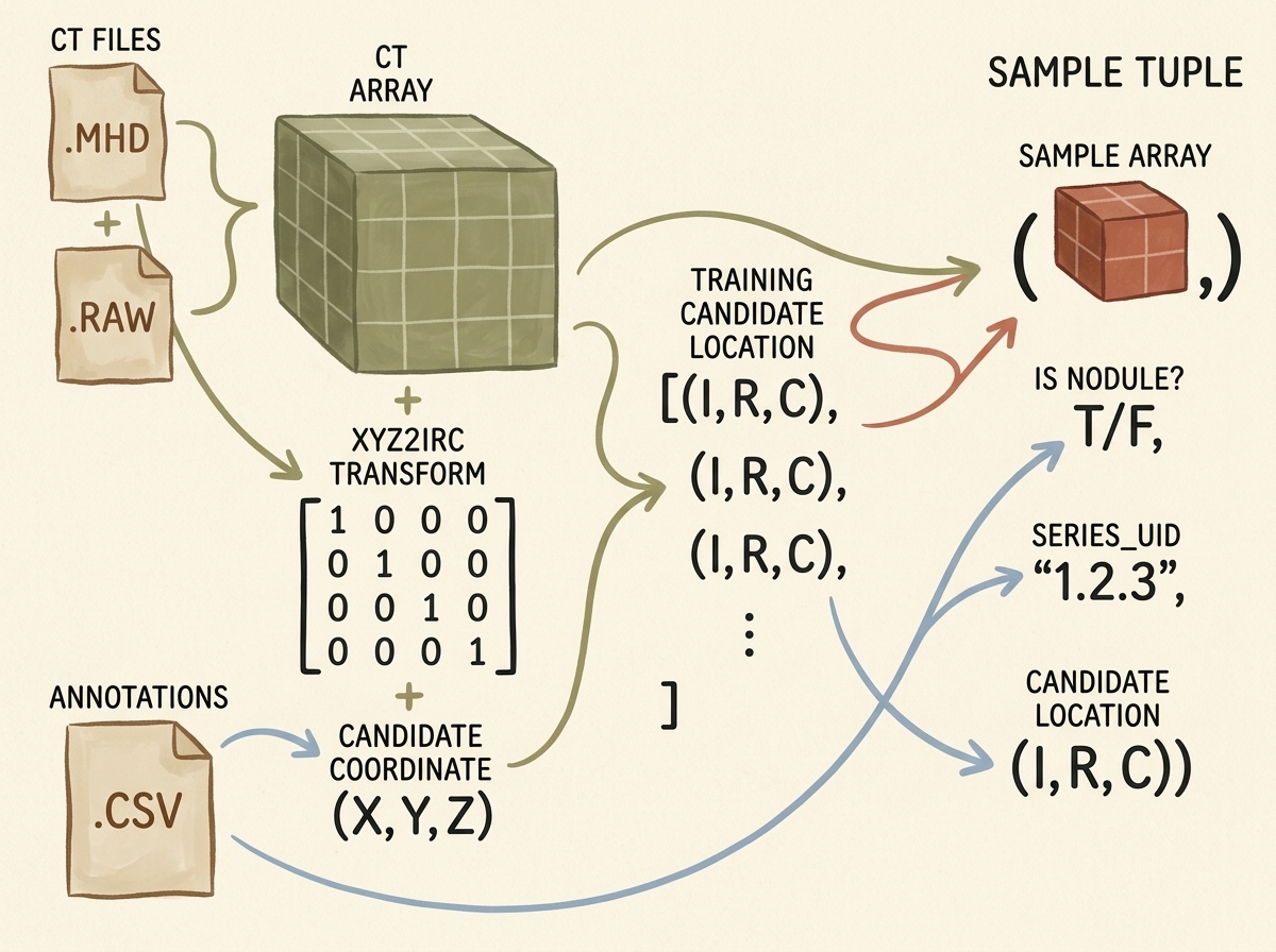
The pipeline constructs an output tuple containing four distinct fields for each candidate item:
candidate_tensor: A $32 \times 32 \times 32$ floating-point tensor crop centered on the candidate nodule location.is_nodule_bool: A boolean ground-truth label ($1$ for genuine nodules, $0$ for non-nodules).series_uid: A unique alphanumeric string identifying the patient scan series.candidate_location_irc: The discrete integer voxel coordinate tuple $(I, R, C)$ identifying the center of the crop.
3. Parsing LUNA Annotation & Candidate Records
3.1 Structure of the Tabular Data
The LUNA Grand Challenge distributes two separate annotation files:
annotations.csv: Contains expert radiologist consensus annotations for confirmed nodules. Each record provides:series_uid: Unique scan identifier.coordX,coordY,coordZ: Center location in continuous millimeters within patient coordinate space.diameter_mm: Approximate sphere diameter of the nodule in millimeters.
candidates.csv: Contains candidate locations produced by candidate generation algorithms (heuristic filters designed for high sensitivity, catching virtually all nodules at the cost of hundreds of thousands of false positives):series_uid: Scan identifier.coordX,coordY,coordZ: Candidate center in millimeters.class: Binary indicator ($1$ for confirmed nodule, $0$ for false-positive non-nodule).
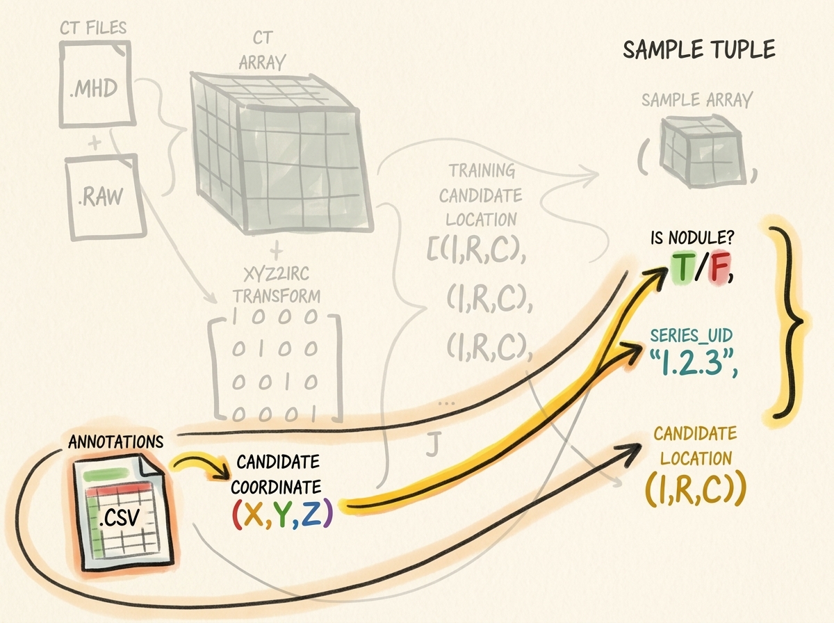
3.2 Unifying Annotations and Candidate Coordinates
Because candidate coordinates generated by detection algorithms rarely match radiologist nodule centers down to the exact sub-millimeter, we merge the two tables by checking if candidate coordinates lie within a bounding sphere of radius $r = \frac{1}{2}\text{diameter\_mm}$ from any confirmed annotation record for the same series_uid.
import csv
import functools
import glob
import os
from collections import namedtuple
# Define clean immutable record types
CandidateInfoTuple = namedtuple(
'CandidateInfoTuple',
['is_nodule_bool', 'diameter_mm', 'series_uid', 'center_xyz']
)
@functools.lru_cache(maxsize=1)
def get_candidate_info_list(require_on_disk_bool=True):
"""
Parses annotations.csv and candidates.csv, merging true nodule diameters
and candidate locations into a single unified list of CandidateInfoTuples.
"""
mhd_list = glob.glob('data-unversioned/part2/luna/subset*/*.mhd')
present_on_disk_set = {os.path.split(p)[-1][:-4] for p in mhd_list}
# Step 1: Ingest true annotations and group by series_uid
diameter_dict = {}
with open('data/part2/luna/annotations.csv', 'r') as f:
for row in list(csv.reader(f))[1:]:
series_uid = row[0]
annotation_center_xyz = tuple(float(x) for x in row[1:4])
annotation_diameter_mm = float(row[4])
diameter_dict.setdefault(series_uid, []).append(
(annotation_center_xyz, annotation_diameter_mm)
)
# Step 2: Ingest all candidates and match with nodule diameters
candidate_info_list = []
with open('data/part2/luna/candidates.csv', 'r') as f:
for row in list(csv.reader(f))[1:]:
series_uid = row[0]
if require_on_disk_bool and series_uid not in present_on_disk_set:
continue
is_nodule_bool = bool(int(row[4]))
candidate_center_xyz = tuple(float(x) for x in row[1:4])
candidate_diameter_mm = 0.0
for annotation_center_xyz, annotation_diameter_mm in diameter_dict.get(series_uid, []):
# Compute Euclidean distance in millimeter space
delta_mm = sum((c - a) ** 2 for c, a in zip(candidate_center_xyz, annotation_center_xyz)) ** 0.5
if delta_mm <= (annotation_diameter_mm / 2.0):
candidate_diameter_mm = annotation_diameter_mm
break
candidate_info_list.append(CandidateInfoTuple(
is_nodule_bool=is_nodule_bool,
diameter_mm=candidate_diameter_mm,
series_uid=series_uid,
center_xyz=candidate_center_xyz
))
# Sort genuine nodules first to facilitate inspection and stratified splits
candidate_info_list.sort(reverse=True)
return candidate_info_list
4. Ingesting Raw CT Scans & The MetaImage Format
4.1 The .mhd and .raw File Structure
A standard CT scan in the LUNA dataset consists of two paired files sharing a common basename:
series_uid.mhd(Meta-Header File): A human-readable text file containing critical volumetric spatial calibration parameters:DimSize = 512 512 215: Number of voxels along $(X, Y, Z)$ or $(C, R, I)$.ElementSpacing = 0.703125 0.703125 1.25: Physical voxel dimensions $(\Delta X, \Delta Y, \Delta Z)$ in millimeters.Offset = -167.3 -172.5 -385.0: Real-world patient coordinate origin corresponding to voxel index $(0, 0, 0)$.TransformMatrix = 1 0 0 0 1 0 0 0 1: Direction cosines matrix describing scanner gantry orientation.ElementType = MET_SHORT: 16-bit signed integer format (int16).
series_uid.raw(Binary Voxel Array): A raw uncompressed binary byte stream containing $512 \times 512 \times 215 \times 2\text{ bytes} \approx 112.7\text{ MB}$ of signed 16-bit integers storing calibrated Hounsfield Units.
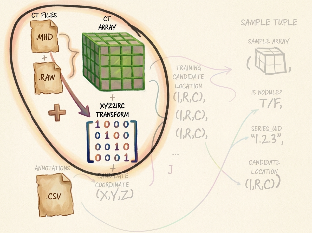
4.2 Reading CT Volumes with SimpleITK
Because NumPy and PyTorch do not natively parse DICOM or MetaImage medical headers, we employ SimpleITK, an industry-standard open-source medical image processing library:
import SimpleITK as sitk
import numpy as np
class Ct:
def __init__(self, series_uid):
mhd_path = glob.glob(f"data-unversioned/part2/luna/subset*/{series_uid}.mhd")[0]
# SimpleITK reads the header metadata and binary stream concurrently
ct_itk = sitk.ReadImage(mhd_path)
# Convert to a 3D NumPy ndarray (float32 for subsequent PyTorch ingestion)
# Note: SimpleITK returns arrays ordered as (Index, Row, Column) -> (Z, Y, X)
ct_array = np.array(sitk.GetArrayFromImage(ct_itk), dtype=np.float32)
# Radiodensity clamping: lung parenchyma sits between -1000 HU (air) and +1000 HU (dense bone)
ct_array.clip(-1000, 1000, ct_array)
self.series_uid = series_uid
self.hu_array = ct_array
self.origin_xyz = tuple(ct_itk.GetOrigin()) # (X, Y, Z) in mm
self.spacing_xyz = tuple(ct_itk.GetSpacing()) # (dX, dY, dZ) in mm
self.direction_matrix = np.array(ct_itk.GetDirection()).reshape(3, 3)
5. Spatial Coordinate Systems & Afin Transformations
Navigating medical volumetric datasets requires mastering two distinct spatial coordinate systems and the mathematical mapping between them.
5.1 The Patient Coordinate System (Millimeter Space)
The Patient Coordinate System (also known as DICOM Patient LPS/RAS space) represents physical anatomy in millimeters:
- Origin $(0, 0, 0)$: Typically calibrated near the center of the scanner gantry or patient thoracic midline.
- $X$-Axis (Left / Right): Positive values point towards the patient’s Left; negative values point to the patient’s Right.
- $Y$-Axis (Posterior / Anterior): Positive values point towards the patient’s Posterior (spine/back); negative values point Anterior (chest/front).
- $Z$-Axis (Superior / Inferior): Positive values point Superior (towards the head); negative values point Inferior (towards the feet).
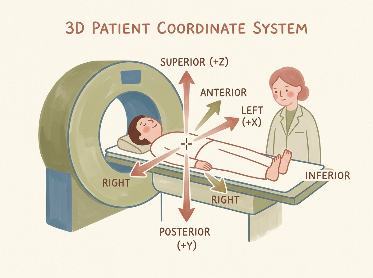
5.2 The Voxel Coordinate System (Array Space)
Unlike continuous millimeters, a computer memory array is indexed by discrete integers $[I, R, C]$:
- $I$ (Index / Slice): Axial slice index along the longitudinal body axis ($Z$).
- $R$ (Row): Vertical matrix index along the coronal/transverse axis ($Y$).
- $C$ (Column): Horizontal matrix index along the sagittal/transverse axis ($X$).
- Array Origin $(0, 0, 0)$: Located at the top-left voxel of the topmost slice.
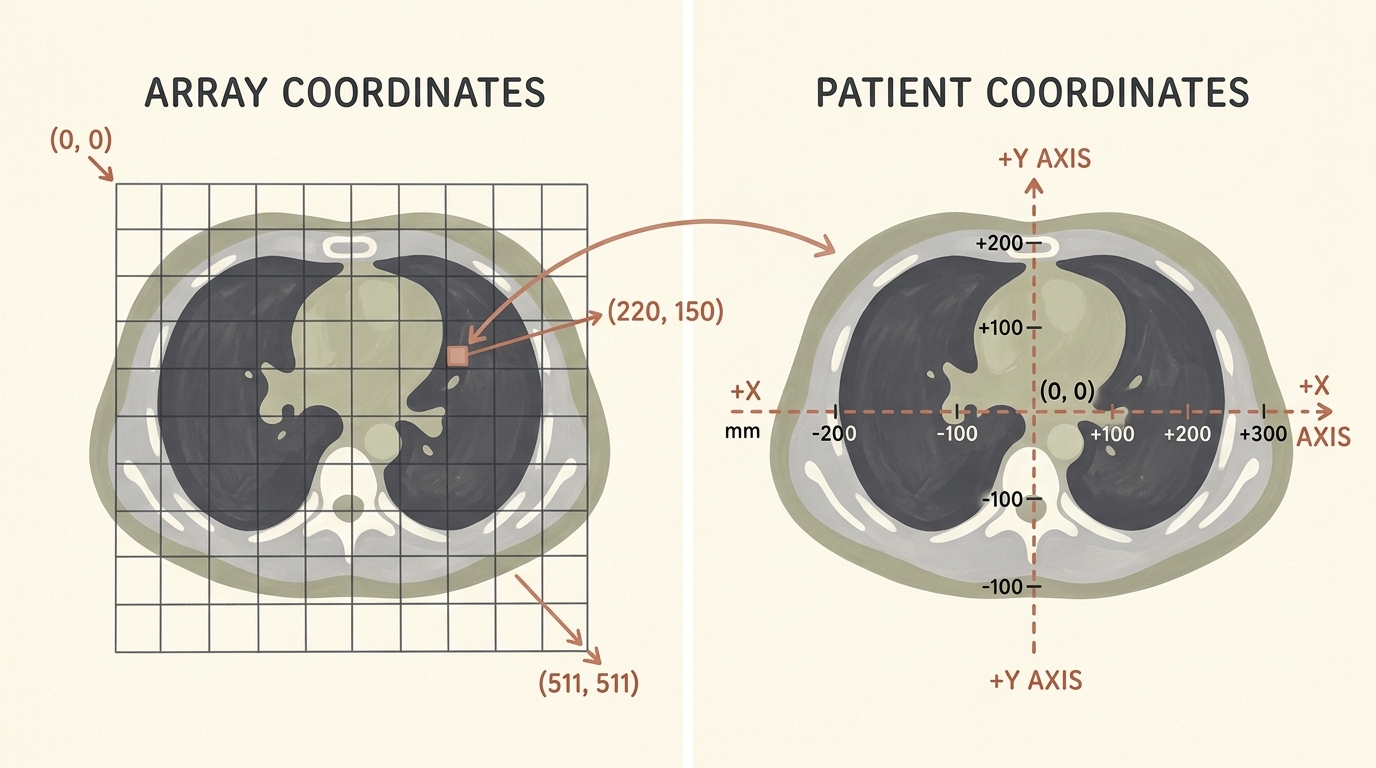
5.3 Mathematical Formulation of Coordinate Transformations
The forward transformation from discrete voxel coordinates $\mathbf{v} = \begin{bmatrix} C & R & I \end{bmatrix}^T$ to continuous patient millimeter space $\mathbf{x} = \begin{bmatrix} X & Y & Z \end{bmatrix}^T$ is governed by an affine transformation:
$$ \begin{bmatrix} X \ Y \ Z \end{bmatrix} = \mathbf{T}_0 + \mathbf{R} \cdot \mathbf{S} \cdot \begin{bmatrix} C \ R \ I \end{bmatrix} $$
Where:
- $\mathbf{T}_0 = \begin{bmatrix} X_0 & Y_0 & Z_0 \end{bmatrix}^T$: The physical millimeter position of origin voxel $(0, 0, 0)$.
- $\mathbf{S} = \text{diag}(\Delta X, \Delta Y, \Delta Z)$: The diagonal voxel spacing matrix representing millimeters per voxel.
- $\mathbf{R}$: The $3 \times 3$ direction cosines rotation matrix ($\mathbf{R} = \mathbf{I}_{3 \times 3}$).
To locate a candidate specified by millimeter coordinates $\mathbf{x} = \begin{bmatrix} X & Y & Z \end{bmatrix}^T$ inside our CT array, we invert this affine mapping:
$$ \begin{bmatrix} C \ R \ I \end{bmatrix} = \text{round}\left( \mathbf{S}^{-1} \cdot \mathbf{R}^{-1} \cdot \left( \begin{bmatrix} X \ Y \ Z \end{bmatrix} - \mathbf{T}_0 \right) \right) $$
Expanding this into component-wise scalar equations:
$$ C = \text{round}\left( \frac{X - X_0}{\Delta X} \right) $$
$$ R = \text{round}\left( \frac{Y - Y_0}{\Delta Y} \right) $$
$$ I = \text{round}\left( \frac{Z - Z_0}{\Delta Z} \right) $$
Key Insight: Notice the coordinate reversal between SimpleITK arrays and patient coordinates! Patient millimeter coordinates are specified in $(X, Y, Z)$, whereas NumPy arrays are indexed in C-order $[I, R, C] \equiv [Z, Y, X]$. Forgetting to reverse indices will transpose patient anatomy, corrupting subsequent convolutions.
from collections import namedtuple
IrcTuple = namedtuple('IrcTuple', ['index', 'row', 'col'])
XyzTuple = namedtuple('XyzTuple', ['x', 'y', 'z'])
def xyz2irc(coord_xyz, origin_xyz, spacing_xyz, direction_matrix):
"""
Transforms continuous patient coordinates (X, Y, Z) in millimeters
into discrete array indices (Index, Row, Col) inside the CT voxel volume.
"""
origin_a = np.array(origin_xyz)
spacing_a = np.array(spacing_xyz)
coord_a = np.array(coord_xyz)
# Invert rotation and translation
difference_a = coord_a - origin_a
current_a = np.dot(np.linalg.inv(direction_matrix), difference_a)
# Scale by voxel spacing and round to nearest integer voxel index
current_a = current_a / spacing_a
cri_a = np.round(current_a).astype(int)
# Return reversed order: (C, R, I) -> (I, R, C)
return IrcTuple(index=int(cri_a[2]), row=int(cri_a[1]), col=int(cri_a[0]))
def irc2xyz(coord_irc, origin_xyz, spacing_xyz, direction_matrix):
"""
Transforms discrete voxel indices (Index, Row, Col) back into
continuous patient millimeter coordinates (X, Y, Z).
"""
# Reverse order: (I, R, C) -> (C, R, I)
cri_a = np.array([coord_irc.col, coord_irc.row, coord_irc.index])
spacing_a = np.array(spacing_xyz)
origin_a = np.array(origin_xyz)
# Scale, rotate, and translate
scaled_a = cri_a * spacing_a
rotated_a = np.dot(direction_matrix, scaled_a)
coord_a = rotated_a + origin_a
return XyzTuple(x=float(coord_a[0]), y=float(coord_a[1]), z=float(coord_a[2]))
6. The Three Orthogonal Anatomical Planes
When examining a 3D thoracic volume, medical imaging software displays cross-sections across three standard orthogonal anatomical planes:
- Axial (Transverse) Plane: Cross-section perpendicular to the spine ($Z$-axis / Index). Slices through the chest from head to toe, viewing lungs from below.
- Coronal (Frontal) Plane: Cross-section parallel to the chest/ribcage ($Y$-axis / Row). Displays lungs and diaphragm domes from the front.
- Sagittal (Lateral) Plane: Vertical cross-section from front to back ($X$-axis / Column). Views the patient from the side, revealing thoracic spine curvature and airway depth.
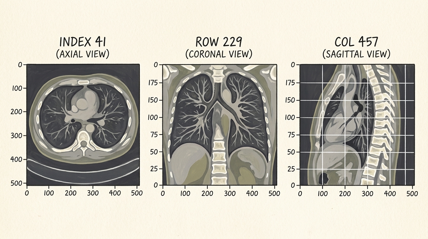
7. Extracting 3D Volumetric Candidate Crops
A full $512 \times 512 \times 300$ CT scan cannot be fed directly into a 3D convolutional neural network during training due to GPU VRAM limits (a single 3D scan at float32 requires hundreds of megabytes of activation memory). Instead, our model operates on localized candidate bounding cubes centered at the candidate’s $(I, R, C)$ coordinate.
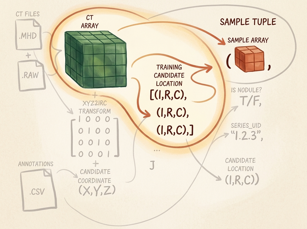
7.1 Slicing and Boundary Handling
We choose a bounding box of size $32 \times 32 \times 32$ voxels (covering roughly $22.5\text{ mm} \times 22.5\text{ mm} \times 40\text{ mm}$ of physical space depending on spacing), which comfortably encapsulates even large $30\text{ mm}$ nodules:
def get_raw_candidate(hu_array, center_irc, width_irc):
"""
Extracts a 3D sub-volume patch of size width_irc centered at center_irc.
Includes boundary clamping to prevent out-of-bounds indexing errors.
"""
slice_list = []
for axis, center_val in enumerate(center_irc):
start_idx = int(round(center_val - width_irc[axis] / 2))
end_idx = int(start_idx + width_irc[axis])
# Clamp bounds to valid array indices
if start_idx < 0:
start_idx = 0
end_idx = int(width_irc[axis])
if end_idx > hu_array.shape[axis]:
end_idx = hu_array.shape[axis]
start_idx = int(end_idx - width_irc[axis])
slice_list.append(slice(start_idx, end_idx))
ct_chunk = hu_array[tuple(slice_list)]
return ct_chunk
8. High-Performance Caching & PyTorch Dataset Architecture
Loading a $100\text{ MB}$ .raw file from spinning disk or NVMe, parsing its metadata with SimpleITK, and extracting a $32^3$ crop takes approximately $1.5\text{ to }3.0\text{ seconds}$ per candidate. With $550{,}000$ candidates, an uncached training loop would take weeks just to complete epoch 0!
To achieve multi-thousand-sample-per-second throughput, we implement a two-tiered caching strategy:
- In-Memory Cache (
functools.lru_cache): Keeps recently accessed full CT volumes in RAM so adjacent candidates from the same patient scan require zero disk I/O. - On-Disk Persistent Cache (
diskcache): Serializes extracted $32 \times 32 \times 32$ float32 chunks directly to an indexed disk cache, bypassing SimpleITK entirely on subsequent epochs.
flowchart TD
Request["LunaDataset.__getitem__(index)"] --> CheckMem{"Candidate In RAM L1 Cache?"}
CheckMem -- Yes --> ReturnMem["Return Voxel Chunk Immediately (<0.1 ms)"]
CheckMem -- No --> CheckDisk{"Chunk In DiskCache L2?"}
CheckDisk -- Yes --> LoadDisk["Load Serialized 32x32x32 Chunk (<2 ms)"]
CheckDisk -- No --> ReadSITK["Read .mhd/.raw with SimpleITK (1.5s - 3.0s)"]
ReadSITK --> ExtractChunk["Extract 32x32x32 Patch & Clip [-1000, 1000]"]
ExtractChunk --> WriteDisk["Write to DiskCache L2"]
WriteDisk --> WriteMem["Store in RAM L1 Cache"]
WriteMem --> ReturnMem
style Request fill:#1a1a2e,stroke:#4cc9f0,stroke-width:2px,color:#fff
style ReturnMem fill:#1a3a2a,stroke:#52b788,stroke-width:2px,color:#fff
style LoadDisk fill:#2a1a3a,stroke:#bd53ed,stroke-width:2px,color:#fff
style ReadSITK fill:#3a1a1a,stroke:#e63946,stroke-width:2px,color:#fff
8.1 Implementing LunaDataset with Zero-Leakage Splitting
import copy
import random
import torch
from torch.utils.data import Dataset
class LunaDataset(Dataset):
def __init__(self,
val_stride=0,
is_val_set_bool=None,
series_uid=None,
sortby_str='random'):
"""
PyTorch Dataset for LUNA candidate nodule patches.
Args:
val_stride (int): Stride for 10-fold patient-wise cross validation (e.g., 10).
is_val_set_bool (bool): If True, yields validation split; if False, yields training split.
series_uid (str): Optional filter to restrict dataset to a single patient scan.
sortby_str (str): Sort order for dataset items ('random', 'series_uid', 'label_and_size').
"""
self.candidate_info_list = copy.copy(get_candidate_info_list())
self.series_uid = series_uid
if series_uid:
self.candidate_info_list = [
x for x in self.candidate_info_list if x.series_uid == series_uid
]
# Critical: Patient-grouped split to prevent data leakage!
# We split based on series_uid rather than candidate indices.
if is_val_set_bool is not None:
assert val_stride > 0, "val_stride must be > 0 when splitting dataset"
if is_val_set_bool:
self.candidate_info_list = [
x for x in self.candidate_info_list
if hash(x.series_uid) % val_stride == 0
]
else:
self.candidate_info_list = [
x for x in self.candidate_info_list
if hash(x.series_uid) % val_stride != 0
]
if sortby_str == 'random':
random.seed(42)
random.shuffle(self.candidate_info_list)
elif sortby_str == 'label_and_size':
self.candidate_info_list.sort(reverse=True)
def __len__(self):
return len(self.candidate_info_list)
def __getitem__(self, ndx):
candidate_info_tup = self.candidate_info_list[ndx]
width_irc = (32, 32, 32)
# get_ct_raw_candidate handles caching and patch slicing
candidate_a, center_irc = get_ct_raw_candidate(
candidate_info_tup.series_uid,
candidate_info_tup.center_xyz,
width_irc
)
# Convert to PyTorch float32 tensor and unsqueeze channel dimension -> (1, D, H, W)
candidate_t = torch.from_numpy(candidate_a).to(torch.float32)
candidate_t = candidate_t.unsqueeze(0)
# Build one-hot target tensor: [non_nodule_prob, nodule_prob]
pos_t = torch.tensor([
not candidate_info_tup.is_nodule_bool,
candidate_info_tup.is_nodule_bool
], dtype=torch.long)
return (
candidate_t,
pos_t,
candidate_info_tup.series_uid,
torch.tensor(center_irc)
)
9. Conclusion & Next Steps
This module completes the foundational data ingestion pipeline of our cancer detection system. By mastering the mathematical bridge between continuous patient millimeters and discrete voxel memory arrays, handling real-world anisotropic CT spacing, and implementing a tiered cache, we transformed a massive, unwieldy 3D medical dataset into clean, uniform PyTorch sample tuples.
In the next module (Section 2.5), we will design and train our first 3D Convolutional Neural Network (nn.Conv3d, nn.MaxPool3d) on top of this LunaDataset, navigating the extreme $99.75%$ class imbalance through customized loss weighting and ROC-AUC evaluation metrics.
Training a Classification Model to Detect Suspected Tumors
- 1. The Cancer Detection Pipeline: Focusing on Classification
- 2. High-Level Training Application Architecture (
LunaTrainingApp) - 3. Pretraining Setup: DataLoaders and Device Management
- 4. 3D Convolutional Neural Network Design (
LunaModel) - 5. Training and Validation Engine
- 6. Metric Tracking and Clinical Performance Logging
- 7. Real-Time Telemetry with TensorBoard
- 8. The Accuracy Paradox: 99.7% Correct and Total Clinical Failure
- 9. Summary and Engineering Principles
1. The Cancer Detection Pipeline: Focusing on Classification
In Section 2.4, we engineered the data ingestion foundation for our clinical diagnostic system: parsing raw thoracic CT scans (.mhd/.raw), mapping continuous millimeter coordinates into discrete voxel matrix indices ($[I, R, C]$), and slicing normalized 3D sub-volume patches ($32 \times 32 \times 32$ voxels) centered on suspicious tissue candidates.
This brings us to Step 3: Nodule Classification in the overall clinical pipeline.
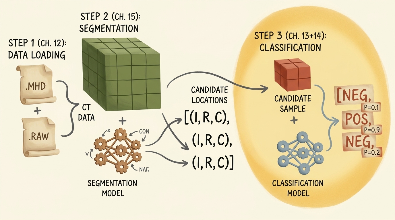
flowchart TD
subgraph Pipeline ["End-to-End Clinical System"]
direction TB
S1["Step 1 (Ch. 12): Volumetric Data Ingestion<br/>CT Reconstruction & Voxel Patch Extraction"]
S2["Step 2 (Ch. 15): Candidate Segmentation<br/>U-Net Anatomical Region Proposals"]
S3["Step 3 (Ch. 13 & 14): Nodule Classification<br/>3D CNN Binary Malignancy Discriminator"]
S1 --> S2 --> S3
end
style Pipeline fill:#1a1a2e,stroke:#4cc9f0,stroke-width:2px,color:#fff
style S1 fill:#16213e,stroke:#4cc9f0,stroke-width:1px,color:#fff
style S2 fill:#1a3a2a,stroke:#52b788,stroke-width:1px,color:#fff
style S3 fill:#3a1a1a,stroke:#e63946,stroke-width:2px,color:#fff
Our primary objective in this module is binary classification: given an extracted volumetric tensor patch of shape $(1, 32, 32, 32)$, predict whether the candidate tissue represents an actual tumor nodule ($y = 1$) or benign non-nodule anatomy ($y = 0$, such as vascular junctions, bronchial walls, or bone spurs).
2. High-Level Training Application Architecture (LunaTrainingApp)
Production-grade deep learning systems require clean, reproducible architectural separation rather than sprawling scripts. We encapsulate the entire training and validation lifecycle within an object-oriented application class: LunaTrainingApp.
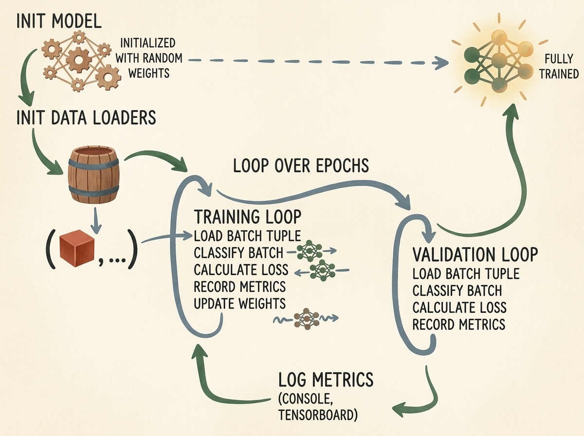
The execution lifecycle follows a structured sequence:
- Command-Line Parsing (
__init__): Parse runtime hyperparameters via Python’s standardargparsemodule (--batch-size,--epochs,--num-workers,--lr). - Resource Setup (
initModel,initOptimizer): Initialize neural network architecture, instantiate optimizers, and bind memory to CUDA or CPU devices. - Data Pipeline Initialization (
initDataLoaders): Build training and validation data loaders with zero-leakage cross-validation grouping. - Epoch Iteration (
main): For each epoch, execute an active gradient-updated training loop (doTraining), followed by an evaluation loop (doValidation) and telemetry logging (logMetrics).
2.1 The Application Scaffold
Let us implement the foundational structure of the training application class:
import argparse
import datetime
import sys
import torch
import torch.nn as nn
from torch.utils.data import DataLoader
from torch.optim import SGD
class LunaTrainingApp:
def __init__(self, sys_argv=None):
if sys_argv is None:
sys_argv = sys.argv[1:]
parser = argparse.ArgumentParser(
description="Train 3D CNN Nodule Classifier on LUNA Dataset."
)
parser.add_argument(
'--batch-size',
help='Batch size to use for training',
default=32,
type=int,
)
parser.add_argument(
'--num-workers',
help='Number of worker processes for background data loading',
default=4,
type=int,
)
parser.add_argument(
'--epochs',
help='Number of epochs to train',
default=1,
type=int,
)
parser.add_argument(
'--tb-prefix',
default='p2ch13',
help="Prefix for TensorBoard run directory",
)
parser.add_argument(
'--comment',
help="Comment suffix for TensorBoard run name",
nargs='?',
default='dwlpt',
)
self.cli_args = parser.parse_args(sys_argv)
self.time_str = datetime.datetime.now().strftime('%Y-%m-%d_%H.%M.%S')
self.use_cuda = torch.cuda.is_available()
self.device = torch.device("cuda" if self.use_cuda else "cpu")
The parameters configured here dictate physical execution:
self.use_cudachecks hardware acceleration. When a CUDA-capable GPU is available, all model weights and input tensor batches are staged into GPU VRAM.self.time_strgenerates an immutable timestamp string for logging directory names, ensuring that different experimental runs never overwrite one another.
3. Pretraining Setup: DataLoaders and Device Management
The preparation phase establishes model weights and data access channels before entering iterative gradient descent.
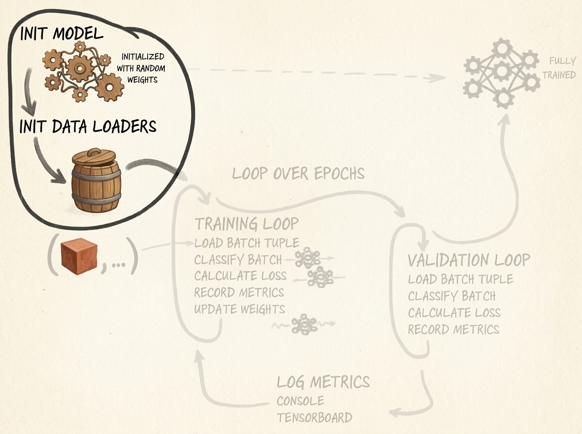
3.1 Initializing the Model and Optimizer
We instantiate the model and move its parameters to the chosen device. We select Stochastic Gradient Descent (SGD) with classical momentum and weight decay:
def initModel(self):
model = LunaModel()
if self.use_cuda:
print(f"Using CUDA device: {torch.cuda.get_device_name(0)}")
if torch.cuda.device_count() > 1:
model = nn.DataParallel(model)
model = model.to(self.device)
return model
def initOptimizer(self):
return SGD(self.model.parameters(), lr=0.001, momentum=0.99)
Note
Setting momentum to
0.99creates substantial exponential averaging of previous gradient vectors: $$ \mathbf{v}_{t} = \mu \mathbf{v}_{t-1} + \mathbf{g}_t, \quad \mathbf{\theta}_{t} = \mathbf{\theta}_{t-1} - \alpha \mathbf{v}_t $$ In sparse gradients where positive nodule samples appear infrequently, high momentum helps push parameters through plateaus, although as we will observe later, this alone cannot overcome extreme class imbalance.
3.2 Care and Feeding of 3D DataLoaders
Each individual call to LunaDataset.__getitem__ yields a 4-element tuple containing a 4D tensor (1, 32, 32, 32), a boolean nodule flag, patient series UID, and physical center coordinate. The DataLoader collates these individual items into batched tensors.
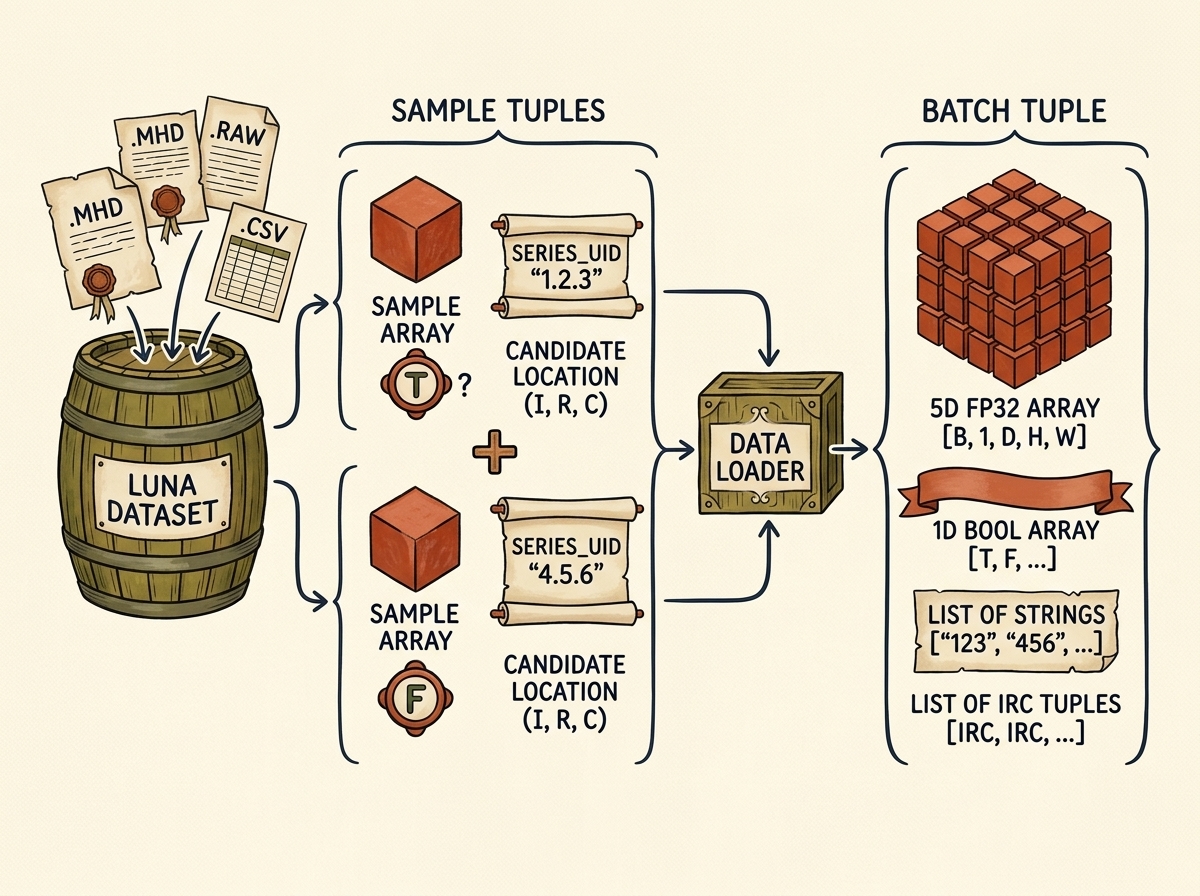
def initTrainDl(self):
train_ds = LunaDataset(
val_stride=10,
is_val_set_bool=False,
)
batch_size = self.cli_args.batch_size
if self.use_cuda:
batch_size *= torch.cuda.device_count()
train_dl = DataLoader(
train_ds,
batch_size=batch_size,
num_workers=self.cli_args.num_workers,
pin_memory=self.use_cuda,
)
return train_dl
def initValDl(self):
val_ds = LunaDataset(
val_stride=10,
is_val_set_bool=True,
)
batch_size = self.cli_args.batch_size
if self.use_cuda:
batch_size *= torch.cuda.device_count()
val_dl = DataLoader(
val_ds,
batch_size=batch_size,
num_workers=self.cli_args.num_workers,
pin_memory=self.use_cuda,
)
return val_dl
Memory & Performance Optimizations:
pin_memory=True: Instructs the runtime to allocate host tensors in page-locked (pinned) system memory. When copying from pinned CPU RAM to CUDA GPU VRAM via.to(self.device, non_blocking=True), the transfer occurs asynchronously via Direct Memory Access (DMA) over the PCIe bus without involving the host CPU core.num_workers=4: Spawns separate worker processes that execute Python unpickling, disk caching lookups, and tensor conversions in parallel background processes, avoiding GPU starvation.val_stride=10: Implements 10-fold patient grouping cross-validation where all candidates belonging to every 10th patient volume are reserved for validation, guaranteeing strict zero data leakage.
4. 3D Convolutional Neural Network Design (LunaModel)
4.1 3D Convolutions: Geometric & Computational Mechanics
In standard 2D image processing, a convolution kernel slides over height and width axes: $(C_{\text{in}}, H, W) \to (C_{\text{out}}, H’, W’)$. In volumetric medical imaging, anatomical nodules are intrinsically 3-dimensional spherical or ellipsoidal structures spanning multiple CT axial slices. Analyzing 2D slices independently discards the critical cross-slice contextual gradient.
A 3D convolution layer (nn.Conv3d) slides a 3D kernel filter across depth ($D$), height ($H$), and width ($W$):
$$ \text{Input Shape: } [N, C, D, H, W] $$
$$\mathbf{Y}_{n, c_{\text{out}}, d, h, w} = \mathbf{b}_{c_{\text{out}}} + \sum_{c_{\text{in}}=0}^{C_{\text{in}}-1} \sum_{i=0}^{K_d-1} \sum_{j=0}^{K_h-1} \sum_{k=0}^{K_w-1} \mathbf{K}_{c_{\text{out}}, c_{\text{in}}, i, j, k} \cdot \mathbf{X}_{n, c_{\text{in}}, d+i, h+j, w+k} $$
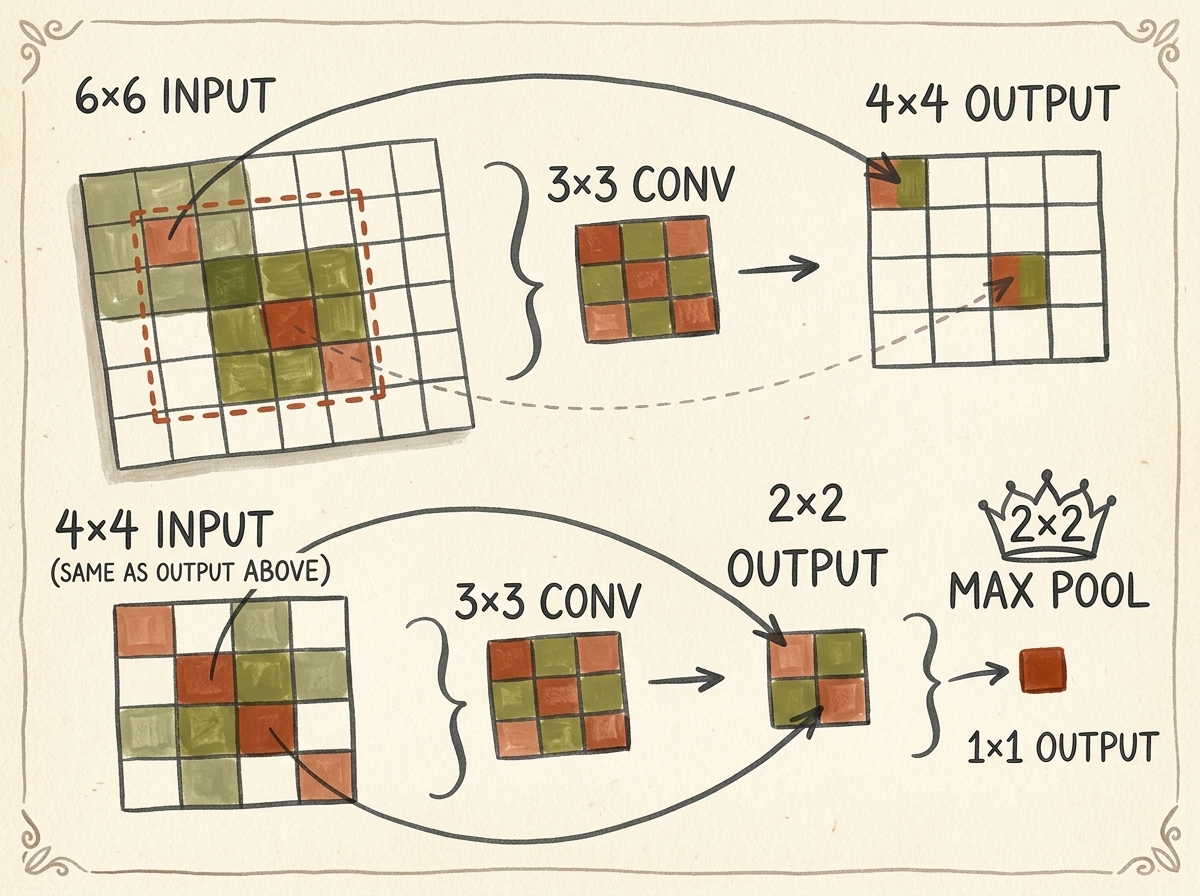
Parameter & Memory Scaling:
- A standard 2D kernel of size $3 \times 3$ contains $9$ weights per channel.
- A 3D kernel of size $3 \times 3 \times 3$ contains $27$ weights per channel—a threefold parameter increase.
- Crucially, activations scale with the volume: an intermediate tensor of shape $[32, 64, 16, 16, 16]$ contains $8{,}388{,}608$ single-precision floating-point elements, consuming $33.55\text{ MB}$ of VRAM for just one layer’s forward activations. Managing spatial downsampling via pooling is essential to prevent GPU out-of-memory crashes.
4.2 Architectural Anatomy of LunaModel
The architecture comprises three primary divisions:
- Tail: An initial
nn.BatchNorm3d(1)that normalizes raw input Hounsfield units on the fly, centering mean around $0$ and variance around $1$. - Backbone: A cascade of 4 modular
LunaBlocksub-networks, progressively increasing channel capacity ($1 \to 8 \to 16 \to 32 \to 64$) while halving spatial resolution at each stage via $2 \times 2 \times 2$ max pooling ($32^3 \to 16^3 \to 8^3 \to 4^3 \to 2^3$). - Head: A linear classification layer mapping the flattened $512$-dimensional embedding vector ($64 \times 2 \times 2 \times 2$) to $2$ output logits, followed by an explicit
nn.Softmax(dim=1)probability distribution: $[\hat{p}_{\text{non-nodule}}, \hat{p}_{\text{nodule}}]$.
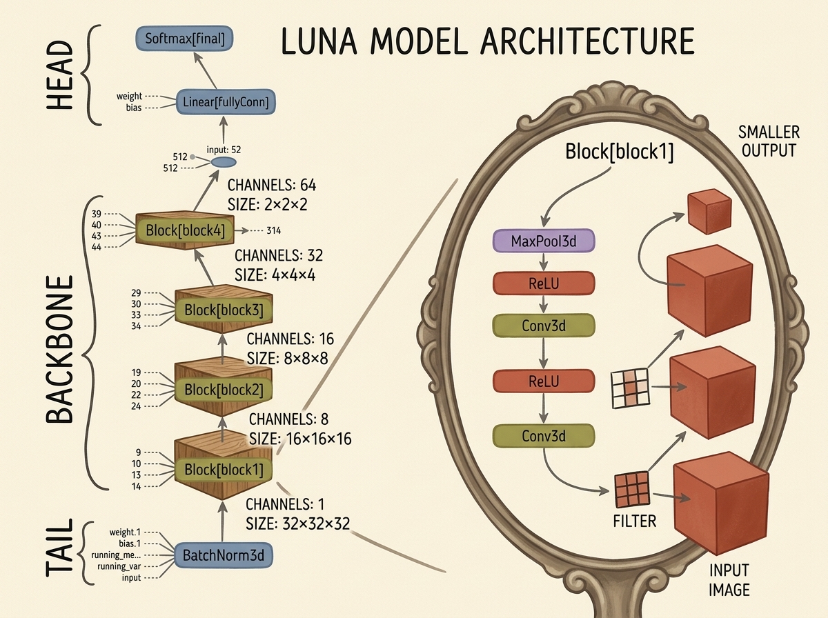
4.3 Implementing LunaBlock and LunaModel
Let us construct the modular network:
class LunaBlock(nn.Module):
def __init__(self, in_channels, conv_channels):
super().__init__()
self.conv1 = nn.Conv3d(
in_channels, conv_channels, kernel_size=3, padding=1, bias=True
)
self.relu1 = nn.ReLU(inplace=True)
self.conv2 = nn.Conv3d(
conv_channels, conv_channels, kernel_size=3, padding=1, bias=True
)
self.relu2 = nn.ReLU(inplace=True)
self.maxpool = nn.MaxPool3d(kernel_size=2, stride=2)
def forward(self, input_batch):
block_out = self.conv1(input_batch)
block_out = self.relu1(block_out)
block_out = self.conv2(block_out)
block_out = self.relu2(block_out)
return self.maxpool(block_out)
Each block maintains spatial dimensions across convolutions through padding=1, reserving all spatial compression for the subsequent nn.MaxPool3d(2, 2) operation.
Now we compose the complete model:
class LunaModel(nn.Module):
def __init__(self):
super().__init__()
self.tail_batchnorm = nn.BatchNorm3d(1)
self.block1 = LunaBlock(1, 8)
self.block2 = LunaBlock(8, 16)
self.block3 = LunaBlock(16, 32)
self.block4 = LunaBlock(32, 64)
self.head_linear = nn.Linear(64 * 2 * 2 * 2, 2)
self.head_softmax = nn.Softmax(dim=1)
self._init_weights()
def _init_weights(self):
for m in self.modules():
if type(m) in {nn.Linear, nn.Conv3d}:
nn.init.kaiming_normal_(
m.weight.data, a=0, mode='fan_out', nonlinearity='relu'
)
if m.bias is not None:
fan_in, _ = nn.init._calculate_fan_in_and_fan_out(m.weight.data)
bound = 1 / (fan_in ** 0.5)
nn.init.uniform_(m.bias.data, -bound, bound)
def forward(self, input_batch):
bn_output = self.tail_batchnorm(input_batch)
conv1_out = self.block1(bn_output)
conv2_out = self.block2(conv1_out)
conv3_out = self.block3(conv2_out)
conv4_out = self.block4(conv3_out)
flattened = conv4_out.view(conv4_out.size(0), -1)
linear_output = self.head_linear(flattened)
return linear_output, self.head_softmax(linear_output)
Notice that forward returns two tensors:
linear_output(raw logits): passed directly to our loss function.self.head_softmax(linear_output)(probabilities): utilized for metric computation, logging, and downstream clinical decision rules.
5. Training and Validation Engine
The training lifecycle alternates between gradient-driven parameter updates (doTraining) and detached evaluation (doValidation).
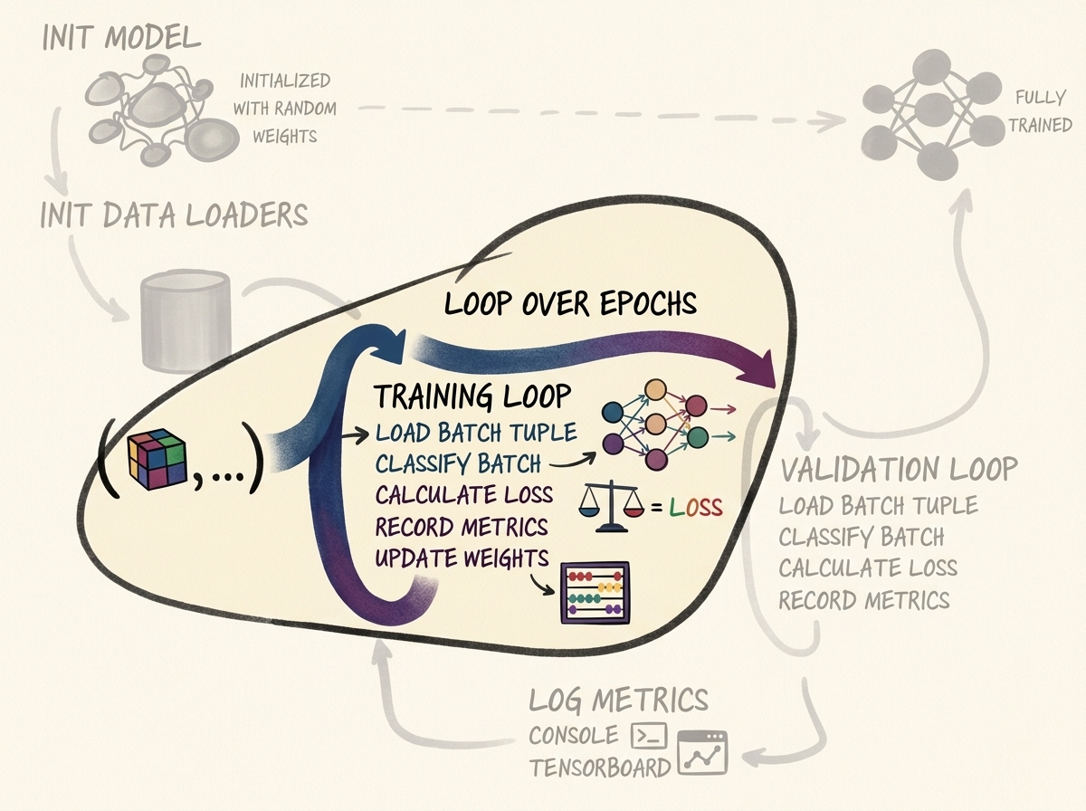
5.1 Computing Batch Loss (computeBatchLoss)
PyTorch’s nn.CrossEntropyLoss expects raw unnormalized logits rather than probabilities, internally combining nn.LogSoftmax with Negative Log-Likelihood (NLLLoss) for numerical stability:
$$ \mathcal{L}_{\text{batch}} = -\frac{1}{B} \sum_{i=1}^{B} \log \left( \frac{\exp(z_{i, y_i})}{\sum_{c=0}^1 \exp(z_{i, c})} \right) $$
def computeBatchLoss(self, batch_ndx, batch_tup, batch_size, trn_metrics_g):
input_t, label_t, _series_list, _center_list = batch_tup
input_dev = input_t.to(self.device, non_blocking=True)
label_dev = label_t.to(self.device, non_blocking=True)
logits_dev, probability_dev = self.model(input_dev)
loss_fn = nn.CrossEntropyLoss(reduction='none')
loss_dev = loss_fn(logits_dev, label_dev)
loss_bool = loss_dev.detach()
probability_bool = probability_dev.detach()
# Update per-sample telemetry tracking matrix
start_ndx = batch_ndx * batch_size
end_ndx = start_ndx + input_t.size(0)
trn_metrics_g[0, start_ndx:end_ndx] = loss_bool
trn_metrics_g[1, start_ndx:end_ndx] = probability_bool[:, 1]
trn_metrics_g[2, start_ndx:end_ndx] = label_dev
return loss_dev.mean()
Important
Always call
.detach()when storing loss values or probabilities into long-term history structures. Storing a live PyTorch tensor preserves its entire backward computational graph in memory, preventing garbage collection and rapidly exhausting system RAM.
5.2 Executing the Training Loop (doTraining)
def doTraining(self, epoch_ndx, train_dl):
self.model.train()
trn_metrics_g = torch.zeros(
3, len(train_dl.dataset), device=self.device
)
for batch_ndx, batch_tup in enumerate(train_dl):
self.optimizer.zero_grad()
loss_var = self.computeBatchLoss(
batch_ndx, batch_tup, train_dl.batch_size, trn_metrics_g
)
loss_var.backward()
self.optimizer.step()
return trn_metrics_g.to('cpu')
5.3 Executing the Validation Loop (doValidation)
In validation, backpropagation must be strictly inhibited to prevent gradient graph construction and reduce memory overhead:
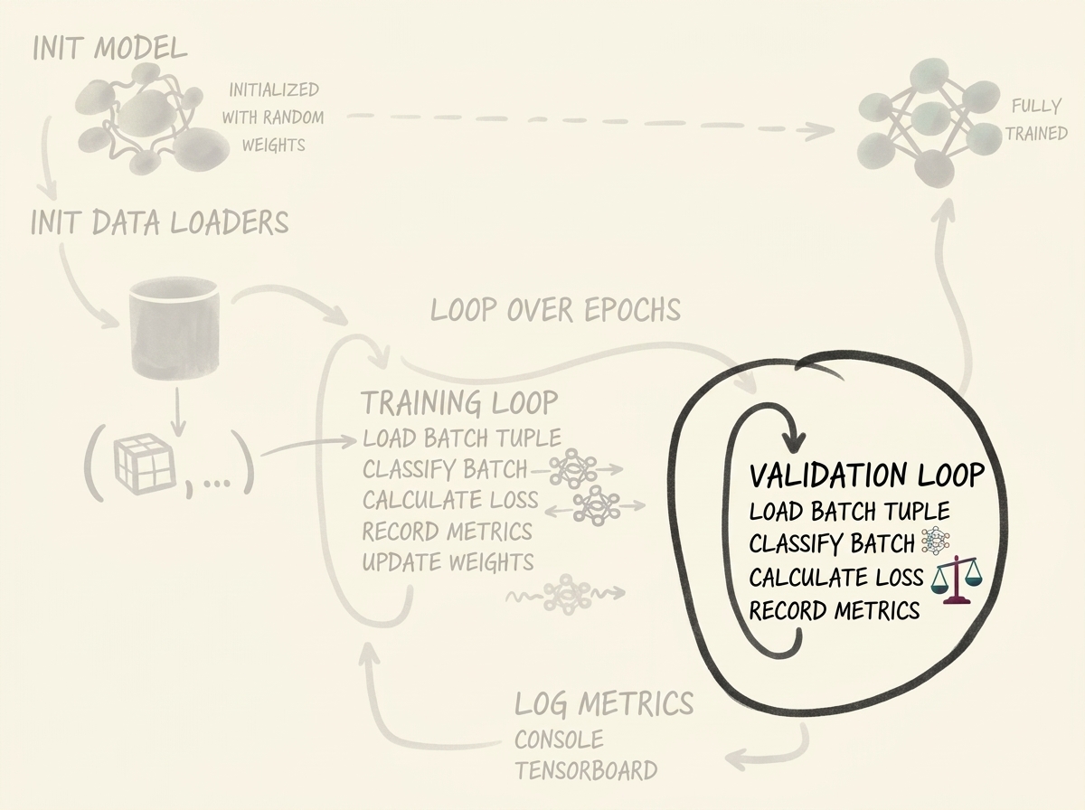
def doValidation(self, epoch_ndx, val_dl):
with torch.inference_mode():
self.model.eval()
val_metrics_g = torch.zeros(
3, len(val_dl.dataset), device=self.device
)
for batch_ndx, batch_tup in enumerate(val_dl):
self.computeBatchLoss(
batch_ndx, batch_tup, val_dl.batch_size, val_metrics_g
)
return val_metrics_g.to('cpu')
6. Metric Tracking and Clinical Performance Logging
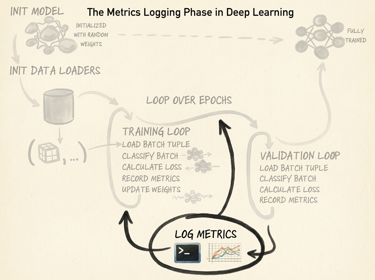
In medical diagnostic applications, overall classification accuracy is an actively hazardous metric. If $99.7%$ of candidates are non-nodules, a dummy model predicting $0$ for every sample achieves $99.7%$ accuracy while allowing $100%$ of malignant cancer patients to go untreated.
We must construct the full Confusion Matrix:
| Condition Positive (True Nodule) | Condition Negative (Benign) | |
|---|---|---|
| Predicted Positive | True Positive (TP) | False Positive (FP) |
| Predicted Negative | False Negative (FN) | True Negative (TN) |
From these four quadrants, we compute clinical diagnostic indicators:
- Sensitivity / Recall: What fraction of genuine nodules did we detect? $$ \text{Recall} = \frac{\text{TP}}{\text{TP} + \text{FN}} $$
- Precision / Positive Predictive Value: When the model flags a nodule, how often is it correct? $$ \text{Precision} = \frac{\text{TP}}{\text{TP} + \text{FP}} $$
- Specificity (True Negative Rate): How accurately does the system dismiss benign tissue? $$ \text{Specificity} = \frac{\text{TN}}{\text{TN} + \text{FP}} $$
- $F_1$-Score: The harmonic mean balancing precision and sensitivity: $$ F_1 = 2 \cdot \frac{\text{Precision} \cdot \text{Recall}}{\text{Precision} + \text{Recall}} $$
Let us implement logMetrics:
def logMetrics(self, epoch_ndx, mode_str, metrics_t):
negLabel_mask = metrics_t[2] == 0
posLabel_mask = metrics_t[2] == 1
negPred_mask = metrics_t[1] < 0.5
posPred_mask = metrics_t[1] >= 0.5
trueNeg_count = (negPred_mask & negLabel_mask).sum().item()
falsePos_count = (posPred_mask & negLabel_mask).sum().item()
truePos_count = (posPred_mask & posLabel_mask).sum().item()
falseNeg_count = (negPred_mask & posLabel_mask).sum().item()
total_count = len(metrics_t[0])
correct_count = trueNeg_count + truePos_count
total_pos = truePos_count + falseNeg_count
total_neg = trueNeg_count + falsePos_count
recall = truePos_count / (total_pos + 1e-8)
precision = truePos_count / (truePos_count + falsePos_count + 1e-8)
f1_score = 2 * (precision * recall) / (precision + recall + 1e-8)
print(
f"Epoch {epoch_ndx} {mode_str:8s} "
f"Loss: {metrics_t[0].mean():.4f} | "
f"Accuracy: {correct_count / total_count * 100:.2f}% | "
f"Recall: {recall * 100:.2f}% | "
f"Precision: {precision * 100:.2f}% | "
f"F1: {f1_score:.4f}"
)
print(
f" TP: {truePos_count:5d} | FN: {falseNeg_count:5d} | "
f"TN: {trueNeg_count:5d} | FP: {falsePos_count:5d}"
)
7. Real-Time Telemetry with TensorBoard
Visualizing training dynamics allows immediate detection of divergence or vanishing gradients. We integrate PyTorch’s native torch.utils.tensorboard.SummaryWriter.
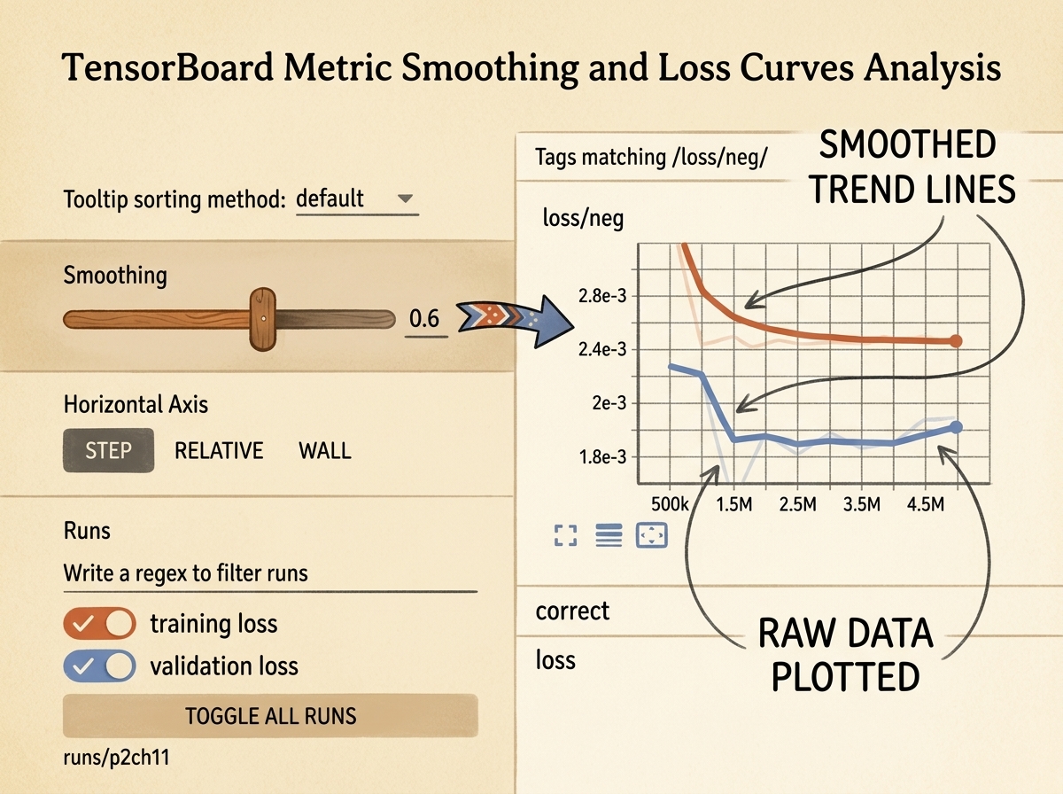
7.1 Initializing the SummaryWriter
from torch.utils.tensorboard import SummaryWriter
def initTensorboard(self):
log_dir = f"runs/{self.cli_args.tb_prefix}_{self.time_str}_{self.cli_args.comment}"
self.trn_writer = SummaryWriter(log_dir=f"{log_dir}_trn")
self.val_writer = SummaryWriter(log_dir=f"{log_dir}_val")
7.2 Writing Scalars to TensorBoard
During logMetrics, we push calculated indicators directly to event logs:
writer = self.trn_writer if mode_str == 'train' else self.val_writer
writer.add_scalar('loss/total', metrics_t[0].mean(), epoch_ndx)
writer.add_scalar('accuracy/overall', correct_count / total_count, epoch_ndx)
writer.add_scalar('clinical/recall', recall, epoch_ndx)
writer.add_scalar('clinical/precision', precision, epoch_ndx)
writer.add_scalar('clinical/f1_score', f1_score, epoch_ndx)
writer.flush()
8. The Accuracy Paradox: 99.7% Correct and Total Clinical Failure
When we execute LunaTrainingApp across the dataset, the console displays a seemingly triumphant result:
Epoch 1 train Loss: 0.0241 | Accuracy: 99.74% | Recall: 0.00% | Precision: 0.00% | F1: 0.0000
TP: 0 | FN: 1351 | TN: 548649 | FP: 0
Epoch 1 val Loss: 0.0238 | Accuracy: 99.76% | Recall: 0.00% | Precision: 0.00% | F1: 0.0000
TP: 0 | FN: 149 | TN: 61251 | FP: 0
8.1 Anatomy of the Catastrophe
-
The Numbers:
- The model achieved an astonishing 99.74% overall accuracy.
- Yet out of $1{,}351$ cancer patients with true nodules, it detected exactly 0 (Zero TP, 1351 FN).
- True Positive Rate (Recall) = 0.00%.
-
Why Did Gradient Descent Choose This? Consider a standard mini-batch of size $32$: $$ \text{Expected Positives per Batch} = 32 \times \frac{1{,}351}{550{,}000} \approx 0.078 \text{ nodules} $$ Out of every $100$ batches processed by the GPU, approximately $92$ batches contain only negative non-nodule samples.
When backpropagation computes gradient vectors across the batch: $$ \nabla_{\mathbf{w}} \mathcal{L} = \frac{1}{B} \sum_{i=1}^B \nabla_{\mathbf{w}} \ell(f(\mathbf{x}_i), y_i) $$ For negative samples ($y_i = 0$), the loss pulls network outputs towards $[1.0, 0.0]$ (class $0$). Because negative samples outnumber positive samples by $400:1$, the sum of negative gradient vectors completely overwhelms and drowns out the occasional positive gradient signal.
The optimizer discovers the simplest, lowest-loss saddle point on the optimization landscape: predict class 0 constantly for all inputs.
flowchart TD
subgraph ImbalanceTrap ["The Class Imbalance Gradient Trap"]
direction TB
B1["Batch N: 32 Benign Samples<br/>Pull weights toward Class 0"]
B2["Batch N+1: 32 Benign Samples<br/>Pull weights toward Class 0"]
B3["Batch N+2: 31 Benign + 1 Nodule<br/>Nodule signal drowned by 31 negative gradients"]
B4["Trivial Local Minimum:<br/>Always predict P(Nodule) = 0.00<br/>Accuracy = 99.74% | Recall = 0.00%"]
B1 --> B2 --> B3 --> B4
end
style ImbalanceTrap fill:#3a1a1a,stroke:#e63946,stroke-width:2px,color:#fff
style B1 fill:#2a1a1a,stroke:#e63946,stroke-width:1px,color:#fff
style B2 fill:#2a1a1a,stroke:#e63946,stroke-width:1px,color:#fff
style B3 fill:#2a1a1a,stroke:#ffaa00,stroke-width:1px,color:#fff
style B4 fill:#1a1a2e,stroke:#4cc9f0,stroke-width:2px,color:#fff
8.2 The Path Forward: Preview of Section 2.6 (Chapter 14)
Overcoming the Accuracy Paradox requires restructuring how our data loaders present reality to the neural network:
- Balanced Stratified Sampling: Enforcing a $1:1$ or $1:3$ ratio of positive nodules to negative samples in every single training batch, ensuring positive gradients have equal voice in weight updates.
- 3D Volumetric Data Augmentation: Because genuine nodules are scarce ($1{,}351$), synthesizing novel samples through 3D rotations, random flips, scaling, and spatial jittering to prevent catastrophic overfitting on balanced splits.
9. Summary and Engineering Principles
- 3D Convolutions Preserve Volumetric Context:
nn.Conv3dprocesses depth, height, and width simultaneously, expanding spatial receptive fields in three dimensions at the cost of cubic parameter and memory scaling. - Decouple Applications into Modular OOP: Isolating initialization (
initModel), data collation (initDataLoaders), loss computation (computeBatchLoss), and metrics tracking (logMetrics) makes training suites scalable and maintainable. - Zero Data Leakage: Ensure training and validation splits group samples by patient UID rather than randomly partitioning isolated candidate patches.
- Accuracy Is Unreliable Under Imbalance: In rare-event detection, high accuracy frequently masks total model collapse. Clinical systems must be evaluated using Confusion Matrices, Recall, Precision, and $F_1$-score.
Improving Training with Metrics and Augmentation
- 1. The Cancer Detection Pipeline: The Accuracy Paradox in Clinical Context
- 2. The 7-Step Improvement Roadmap
- 3. The Guard Dog Metaphor: Intuition Behind Binary Classification
- 4. Mathematical Formulation of Clinical Evaluation Metrics
- 5. Engineering the Telemetry Engine (
logMetrics) - 6. What Does an Ideal Dataset Look Like?
- 7. Step 5: Implementing Balanced Dataset Sampling
- 8. The Symptom of Overfitting: When Balanced Training Backfires
- 9. Step 6: 3D Volumetric Data Augmentation Pipeline
- 10. Experimental Results: Before vs. After Augmentation
- 11. Summary and Engineering Principles
1. The Cancer Detection Pipeline: The Accuracy Paradox in Clinical Context
In Section 2.5, we implemented our baseline 3D Convolutional Neural Network (LunaModel) and discovered the Accuracy Paradox: our model achieved a seemingly triumphant 99.74% overall classification accuracy, yet in clinical practice it was an absolute failure. Out of $1{,}351$ genuine malignant tumor candidates, the network identified exactly 0 (Zero True Positives, 1351 False Negatives).
To understand why this happened and how to engineer a viable clinical tool, we must place our classification model back inside the end-to-end Computer-Aided Detection (CAD) pipeline.
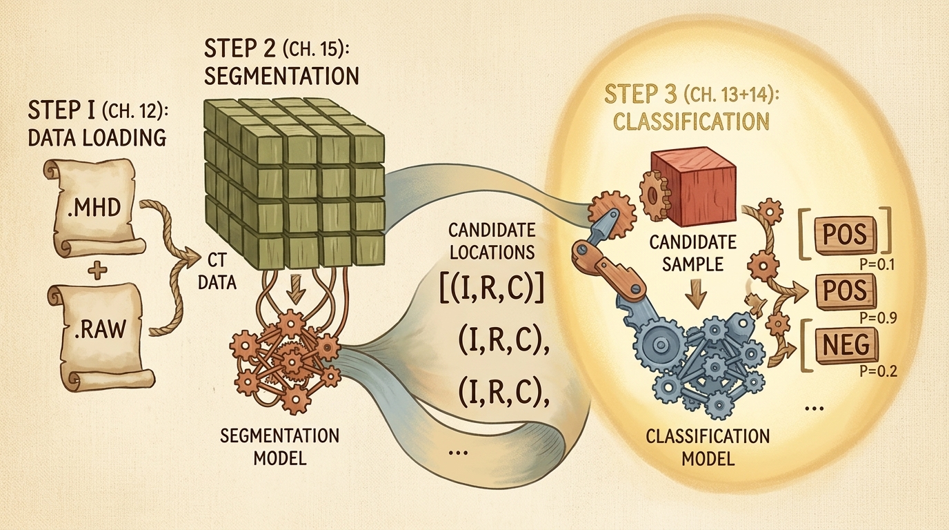
flowchart TD
subgraph CADPipeline ["Clinical CAD Detection Workflow"]
direction TB
S1["Step 1: Volumetric Ingestion<br/>DICOM/MHD Scans to Voxel Tensors"]
S2["Step 2: Region Proposals<br/>Candidate Segmentation Model"]
S3["Step 3: Nodule Classification<br/>3D CNN Binary Discriminator"]
S1 --> S2 --> S3
end
style CADPipeline fill:#1a1a2e,stroke:#4cc9f0,stroke-width:2px,color:#fff
style S1 fill:#16213e,stroke:#4cc9f0,stroke-width:1px,color:#fff
style S2 fill:#1a3a2a,stroke:#52b788,stroke-width:1px,color:#fff
style S3 fill:#3a1a1a,stroke:#e63946,stroke-width:2px,color:#fff
In medical screening, an asymmetric cost matrix governs diagnostic utility:
- False Negative (FN): A malignant nodule is incorrectly classified as benign tissue. The patient is sent home without intervention, the cancer metastasizes, and the opportunity for early curative surgical resection is lost. The clinical cost is catastrophic.
- False Positive (FP): Benign anatomical structures (blood vessels, lymph nodes, or pleural scarring) are flagged as suspicious tumors. The patient undergoes a secondary high-resolution scan, biopsy, or bronchoscopy. While causing anxiety and procedural cost, the patient remains alive.
A model that predicts negative for every candidate avoids false positives entirely and maximizes raw percentage accuracy, but it is biologically and medically useless.
2. The 7-Step Improvement Roadmap
To transition from our failed baseline model to a high-performance clinical screening system, we follow a rigorous seven-stage engineering plan.
flowchart TD
subgraph Roadmap ["Engineering Improvement Sequence"]
direction TB
R1["1. Guard Dogs Intuition<br/>Threshold Mechanics & Decision Boundaries"]
R2["2. Birds & Burglars Framing<br/>Asymmetric Signal & Noise Separation"]
R3["3. Metrics Ratios<br/>Formalizing Recall & Precision"]
R4["4. The Harmonic F1 Score<br/>A Single Truthful Health Metric"]
R5["5. Dataset Balancing<br/>Stratified Dynamic Mini-Batch Sampling"]
R6["6. 3D Data Augmentation<br/>Affine Rotations, Scaling, and Noise"]
R7["7. Verified Clinical Screener<br/>Stable Loss & Converged Precision-Recall"]
R1 --> R2 --> R3 --> R4 --> R5 --> R6 --> R7
end
style Roadmap fill:#1a1a2e,stroke:#4cc9f0,stroke-width:2px,color:#fff
style R1 fill:#16213e,stroke:#4cc9f0,stroke-width:1px,color:#fff
style R2 fill:#16213e,stroke:#4cc9f0,stroke-width:1px,color:#fff
style R3 fill:#16213e,stroke:#4cc9f0,stroke-width:1px,color:#fff
style R4 fill:#2b2d42,stroke:#ffaa00,stroke-width:1px,color:#fff
style R5 fill:#2b2d42,stroke:#e63946,stroke-width:1px,color:#fff
style R6 fill:#2b2d42,stroke:#52b788,stroke-width:1px,color:#fff
style R7 fill:#0f3460,stroke:#4cc9f0,stroke-width:2px,color:#fff
We begin by establishing the mathematical and operational framework through Steps 1, 2, and 3.
3. The Guard Dog Metaphor: Intuition Behind Binary Classification
To build an intuitive foundation for classification thresholds under severe noise, consider a homeowner employing a guard dog to protect a property from burglars.
In this metaphor:
- Intruders / Burglars: Positive class ($y = 1$, actual tumors).
- Innocent Wildlife (Birds, Cats, Rabbits): Negative class ($y = 0$, benign tissue).
- Dog Barks: Positive prediction ($\hat{y} = 1$).
- Dog Ignores / Sleeps: Negative prediction ($\hat{y} = 0$).
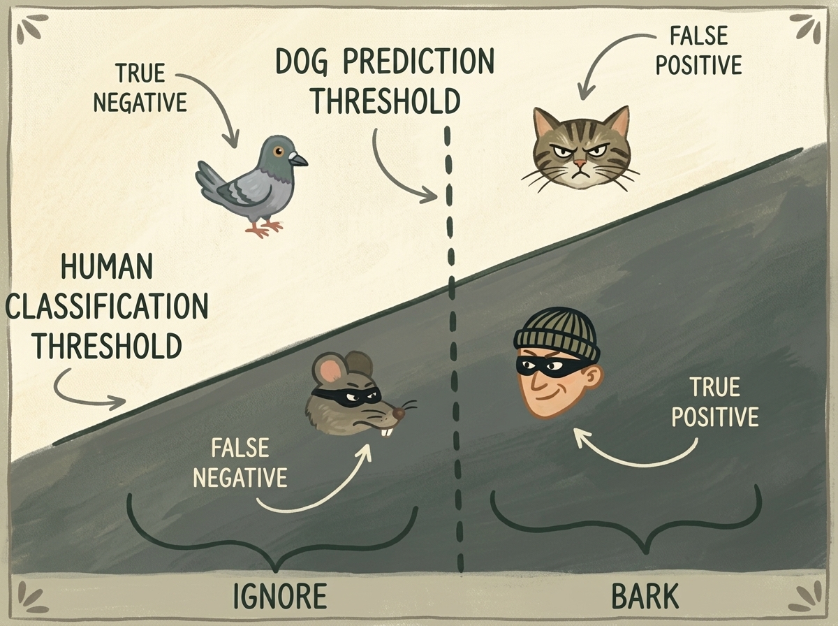
The operational space is bifurcated into four quadrants:
- True Negative ($TN$): A bird flutters into the garden; the dog stays quiet. No alarm, no intruder. Correct decision.
- False Positive ($FP$): An alley cat rustles a hedge; the dog barks frantically. Homeowner awakens in panic for a non-threat. False alarm.
- False Negative ($FN$): A masked burglar tiptoes across the lawn; the dog snores quietly. Total security failure.
- True Positive ($TP$): A burglar enters; the dog barks vigorously. The threat is identified and neutralized.
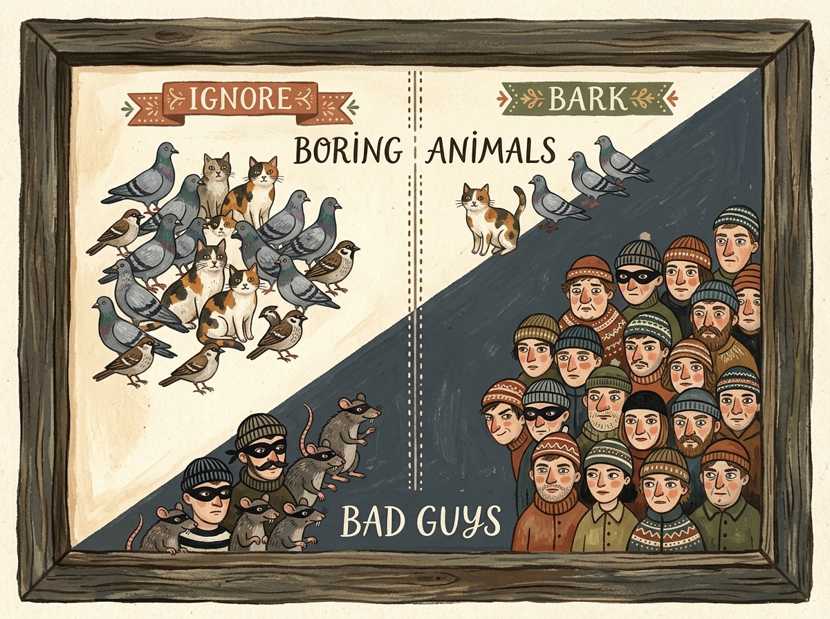
3.1 The Two Extremes: Chirpy vs. Dozer
A classification model does not output a binary ${0, 1}$ label directly; it outputs continuous logits $\mathbf{z} \in \mathbb{R}^2$, transformed via softmax into posterior probabilities $\hat{p} = P(y = 1 \mid \mathbf{x}) \in [0, 1]$. The decision rule compares $\hat{p}$ against a chosen threshold $\tau$: $$ \hat{y} = \begin{cases} 1 & \text{if } \hat{p} \ge \tau \ 0 & \text{if } \hat{p} < \tau \end{cases} $$
The choice of threshold $\tau$ exposes a fundamental trade-off embodied by two archetypal guard dogs:
Archetype A: Chirpy (The Overzealous Terrier)
Chirpy barks at fallen leaves, shadows, wind gusts, and passing cars ($\tau \to 0.0$).
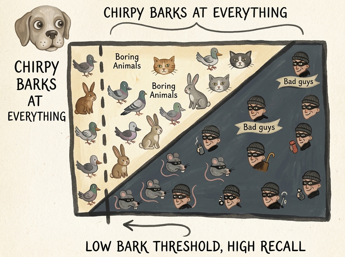
- Strength: No burglar ever sneaks past. $FN = 0 \implies \text{Recall} = 100%$.
- Weakness: The homeowner is awakened 40 times a night. Every alarm is assumed to be noise. $FP$ is astronomical $\implies \text{Precision} \to 0%$.
Archetype B: Dozer (The Lethargic Mastiff)
Dozer sleeps on the porch 23 hours a day. He only barks if someone violently kicks his dog bowl ($\tau \to 1.0$).
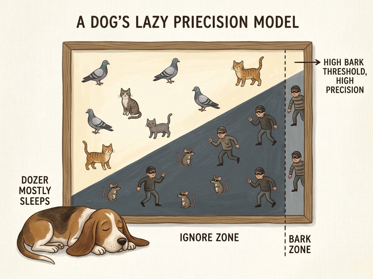
- Strength: When Dozer barks, you grab a shotgun immediately—he is never wrong. $FP \approx 0 \implies \text{Precision} \to 100%$.
- Weakness: 10 burglars emptied the garage while he slept. $FN$ is massive $\implies \text{Recall} \to 0%$.
Our baseline model from Section 2.5 was an extreme version of Dozer: it achieved $99.74%$ accuracy by permanently sleeping and never barking at a single tumor.
4. Mathematical Formulation of Clinical Evaluation Metrics
To evaluate model performance objectively, we abandon overall accuracy and compute the full Confusion Matrix:
| Ground Truth Positive ($y=1$) | Ground Truth Negative ($y=0$) | |
|---|---|---|
| Predicted Positive ($\hat{y}=1$) | $\text{TP}$ | $\text{FP}$ |
| Predicted Negative ($\hat{y}=0$) | $\text{FN}$ | $\text{TN}$ |
4.1 Sensitivity (Recall / True Positive Rate)
Recall answers the vital clinical question: Out of all patients who actually harbor a malignant nodule, what percentage did our algorithm detect?
$$ \text{Recall} = \frac{\text{TP}}{\text{TP} + \text{FN}} $$
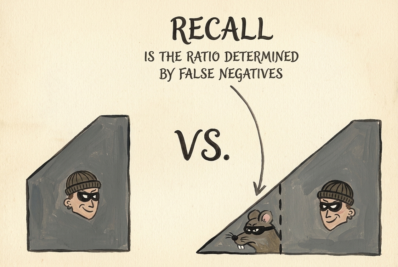
When False Negatives ($\text{FN}$) increase, Recall plummets toward zero. In cancer screening, Recall is our primary non-negotiable health safety threshold.
4.2 Precision (Positive Predictive Value)
Precision answers the diagnostic credibility question: When our neural network raises an alarm and flags a volumetric candidate as a tumor, how often is it actually correct?
$$ \text{Precision} = \frac{\text{TP}}{\text{TP} + \text{FP}} $$
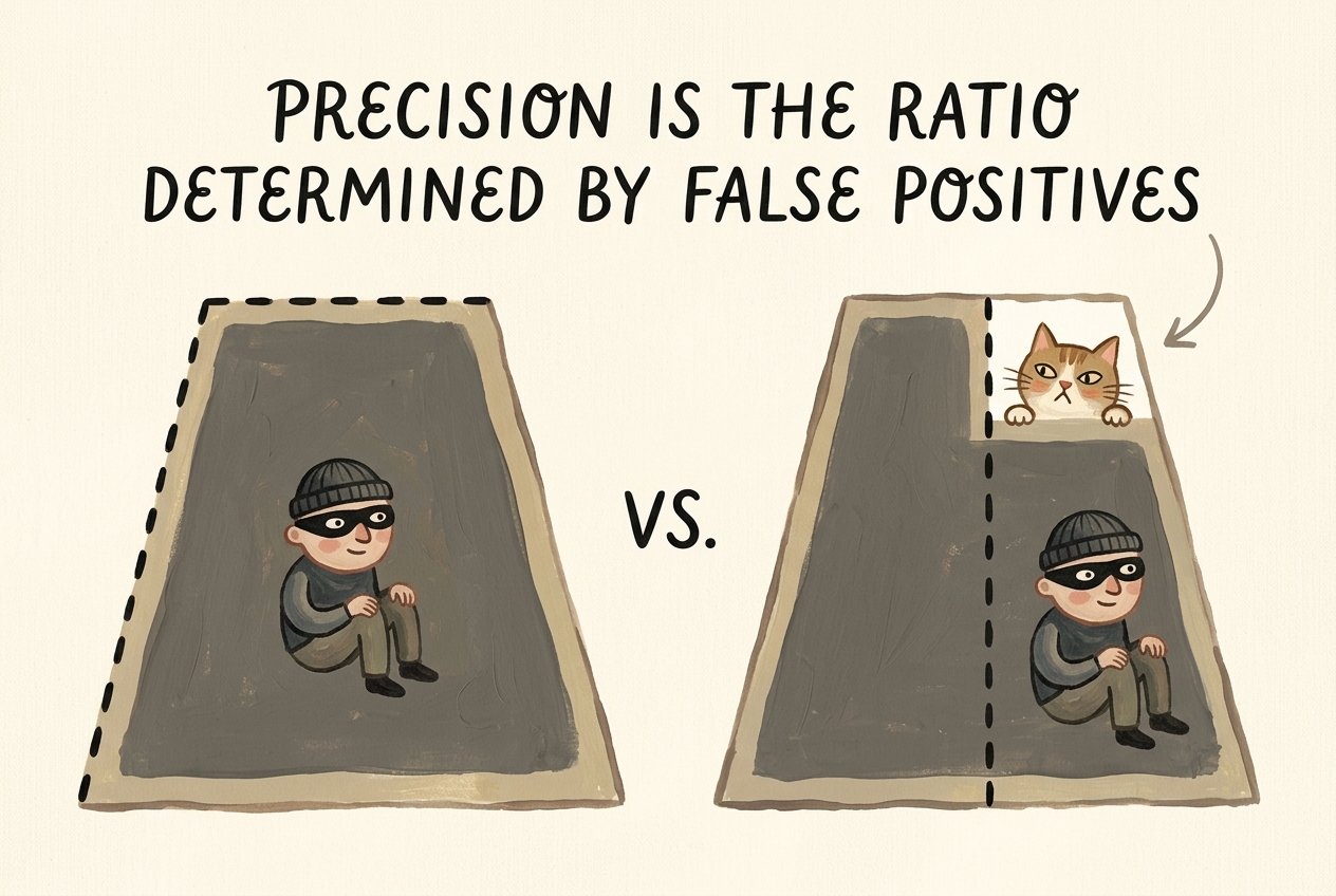
When False Positives ($\text{FP}$) increase, Precision drops. Low precision leads to clinical alarm fatigue, unnecessary surgical biopsies, and high patient distress.
4.3 Specificity (True Negative Rate)
Specificity quantifies how cleanly the system dismisses healthy tissue:
$$ \text{Specificity} = \frac{\text{TN}}{\text{TN} + \text{FP}} $$
Under extreme class imbalance where negative candidates outnumber positive nodules $400:1$, Specificity can easily read $99.5%$ while precision remains below $5%$, because even $0.5%$ false positives among $550{,}000$ benign samples creates $2{,}750$ false alarms—drowning out the $1{,}351$ true nodules.
4.4 The Harmonic Mean: The $F_1$-Score
We need a single scalar indicator that balances Precision ($P$) and Recall ($R$). If we were to use the simple arithmetic mean: $$ A(P, R) = \frac{P + R}{2} $$ A degenerate model with $P = 0.0$ and $R = 1.0$ (barking at everything) would receive an unearned score of $0.50$ ($50%$).
Instead, we compute the $F_1$-score, which is the Harmonic Mean of Precision and Recall:
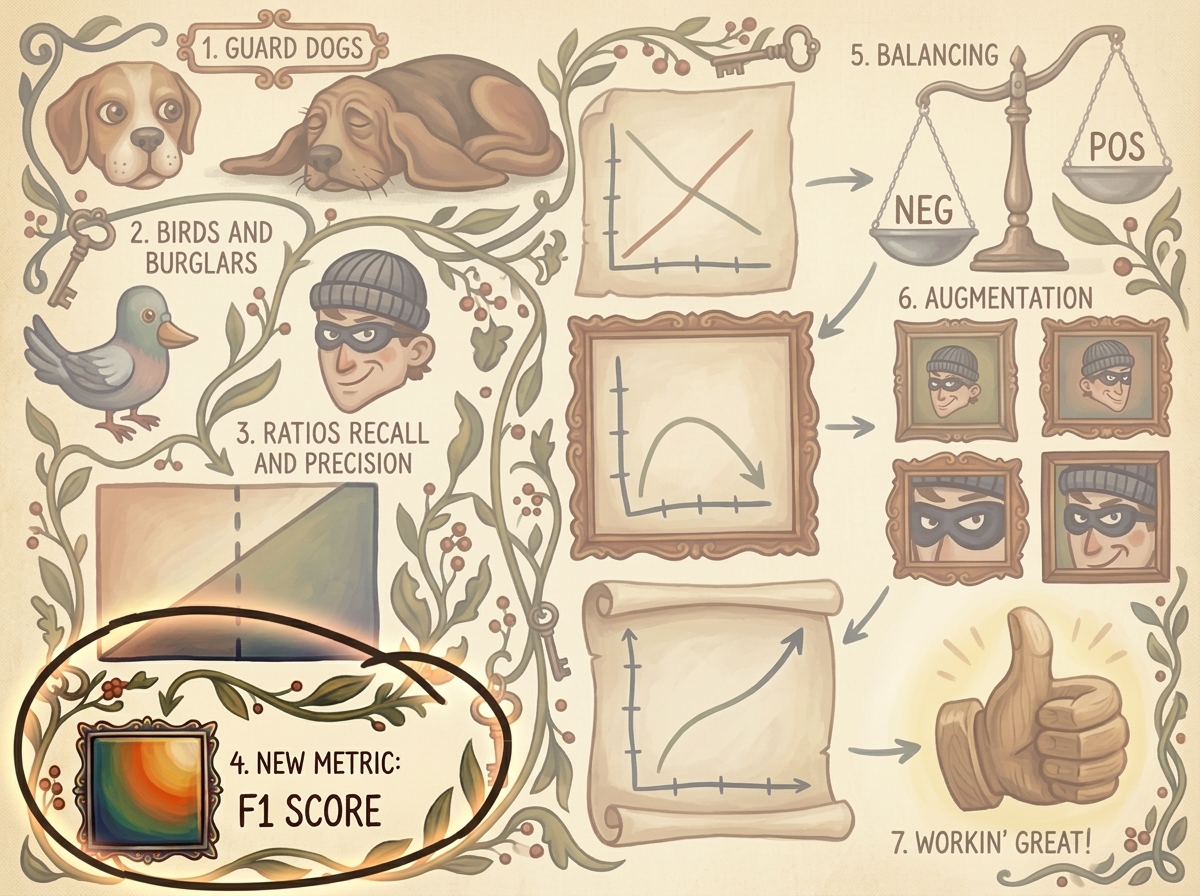
$$ F_1 = 2 \cdot \frac{P \cdot R}{P + R} = \frac{2\text{TP}}{2\text{TP} + \text{FP} + \text{FN}} $$
Mathematical Proof of Harmonic Penalty:
Recall the arithmetic-harmonic inequality: for any positive real values $x, y > 0$:
$$ H(x, y) = \frac{2}{\frac{1}{x} + \frac{1}{y}} = \frac{2xy}{x+y} \le \frac{x+y}{2} = A(x, y) $$
With equality if and only if $x = y$.
Crucially, as either $P \to 0$ or $R \to 0$:
$$ \lim_{P \to 0} F_1(P, R) = \lim_{P \to 0} \frac{2 P R}{P + R} = 0 $$
The harmonic mean forces the metric to zero if either precision or recall collapses. A model cannot achieve a respectable $F_1$-score by sacrificing one metric entirely.
5. Engineering the Telemetry Engine (logMetrics)
Let us upgrade our logMetrics method inside LunaTrainingApp to compute and report these clinical metrics dynamically across training and validation splits.
import torch
def logMetrics(self, epoch_ndx, mode_str, metrics_t, classificationThreshold=0.5):
"""
Computes confusion matrix, recall, precision, and F1-score across batched tensors.
metrics_t layout:
Row 0: Loss values per sample
Row 1: Positive class predicted probabilities (P(nodule))
Row 2: Ground truth binary labels (0 or 1)
"""
negLabel_mask = metrics_t[2] == 0
posLabel_mask = metrics_t[2] == 1
negPred_mask = metrics_t[1] < classificationThreshold
posPred_mask = metrics_t[1] >= classificationThreshold
trueNeg_count = (negPred_mask & negLabel_mask).sum().item()
falsePos_count = (posPred_mask & negLabel_mask).sum().item()
truePos_count = (posPred_mask & posLabel_mask).sum().item()
falseNeg_count = (negPred_mask & posLabel_mask).sum().item()
total_count = len(metrics_t[0])
correct_count = trueNeg_count + truePos_count
total_pos = truePos_count + falseNeg_count
total_neg = trueNeg_count + falsePos_count
recall = truePos_count / (total_pos + 1e-8)
precision = truePos_count / (truePos_count + falsePos_count + 1e-8)
f1_score = 2 * (precision * recall) / (precision + recall + 1e-8)
specificity = trueNeg_count / (total_neg + 1e-8)
print(
f"Epoch {epoch_ndx:2d} {mode_str:6s} "
f"Loss: {metrics_t[0].mean():.4f} | "
f"Acc: {correct_count / total_count * 100:.2f}% | "
f"Recall: {recall * 100:.2f}% | "
f"Prec: {precision * 100:.2f}% | "
f"F1: {f1_score:.4f}"
)
print(
f" TP: {truePos_count:5d} | FN: {falseNeg_count:5d} | "
f"TN: {trueNeg_count:5d} | FP: {falsePos_count:5d}"
)
# Push per-class losses and performance metrics to TensorBoard
writer = self.trn_writer if mode_str == 'train' else self.val_writer
writer.add_scalar('loss/all', metrics_t[0].mean(), epoch_ndx)
writer.add_scalar('loss/neg', metrics_t[0, negLabel_mask].mean(), epoch_ndx)
if posLabel_mask.any():
writer.add_scalar('loss/pos', metrics_t[0, posLabel_mask].mean(), epoch_ndx)
writer.add_scalar('pr/recall', recall, epoch_ndx)
writer.add_scalar('pr/precision', precision, epoch_ndx)
writer.add_scalar('pr/f1_score', f1_score, epoch_ndx)
writer.flush()
6. What Does an Ideal Dataset Look Like?
Before resolving our data problems, let us conceptualize what an ideal training distribution looks like versus the harsh reality of medical CT scans.
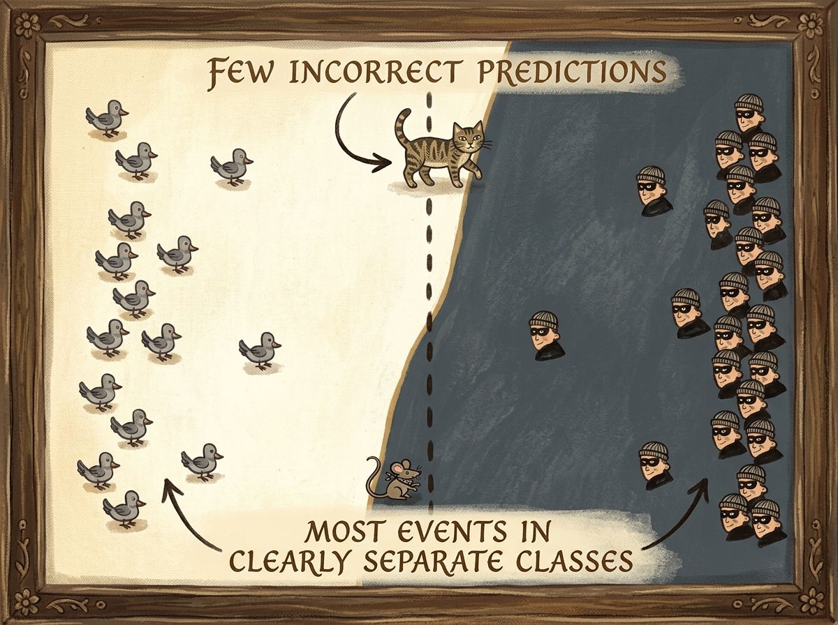
In an ideal dataset:
- Both classes have abundant representations ($\sim 50%$ positives, $\sim 50%$ negatives).
- The intrinsic features (voxel density gradients, sphericity, tissue texture) exhibit high inter-class variance and low intra-class variance.
- Every mini-batch contains a steady, balanced mixture of both categories.
6.1 The Real-World Reality: Catastrophic Asymmetry
In clinical reality, thoracic CT scans present a radically skewed landscape:
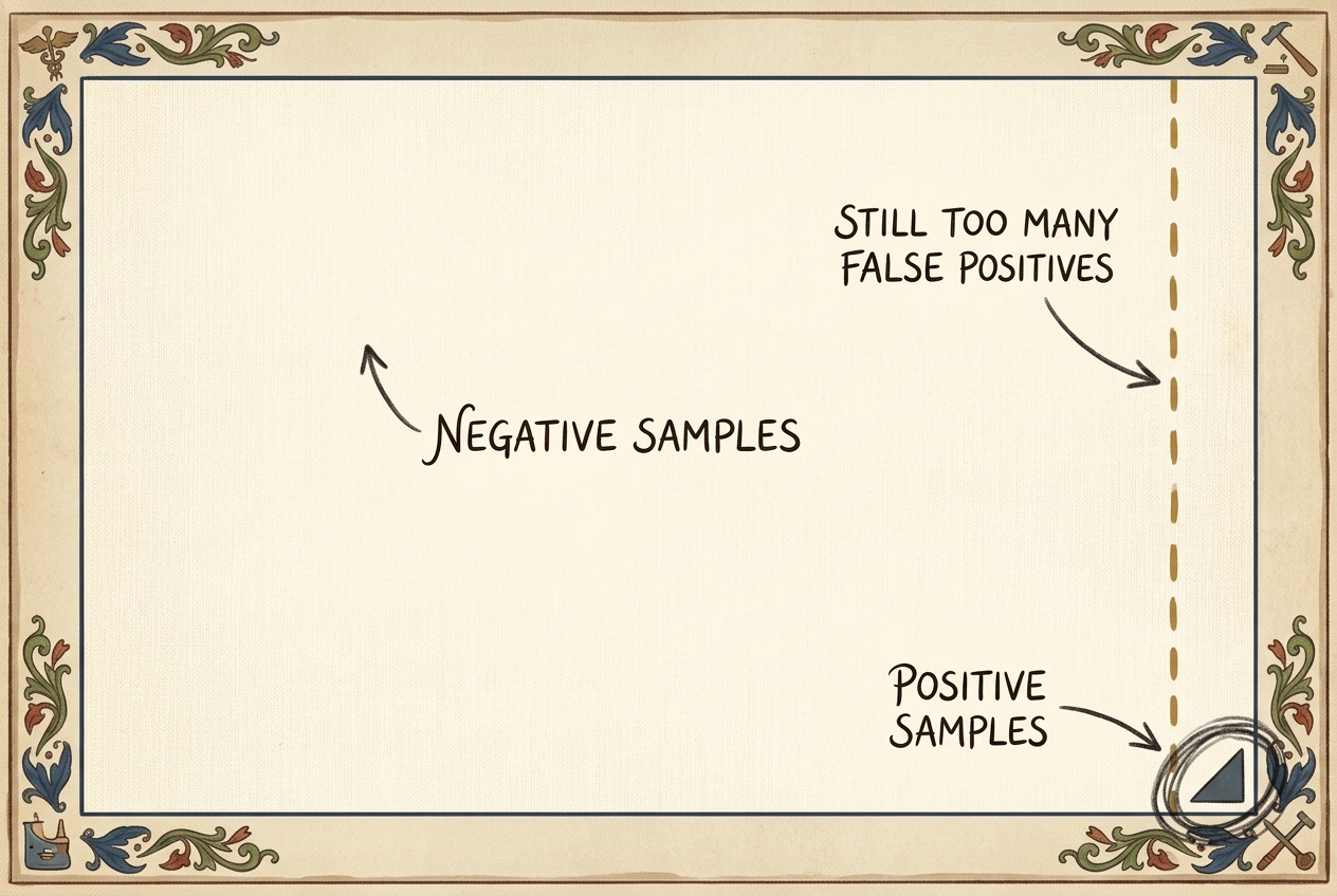
In the LUNA dataset:
- Total candidate patches: $\approx 551{,}065$
- Genuine tumor nodules: $1{,}351$ ($0.245%$)
- Benign non-nodules: $549{,}714$ ($99.755%$)
- Imbalance ratio: $\approx 407 : 1$
6.2 Mini-Batch Starvation
When training a neural network with Stochastic Gradient Descent using mini-batches of size $B = 32$, the probability distribution of nodules per batch follows a binomial distribution: $$ X \sim \text{Binomial}(B = 32, p = 0.00245) $$ The expected number of nodules in any given batch is: $$ \mathbb{E}[X] = B \cdot p = 32 \times 0.00245 \approx 0.0784 \text{ nodules} $$
The probability that a mini-batch contains zero nodules: $$ P(X = 0) = (1 - 0.00245)^{32} \approx 0.9246 \quad (92.46%) $$
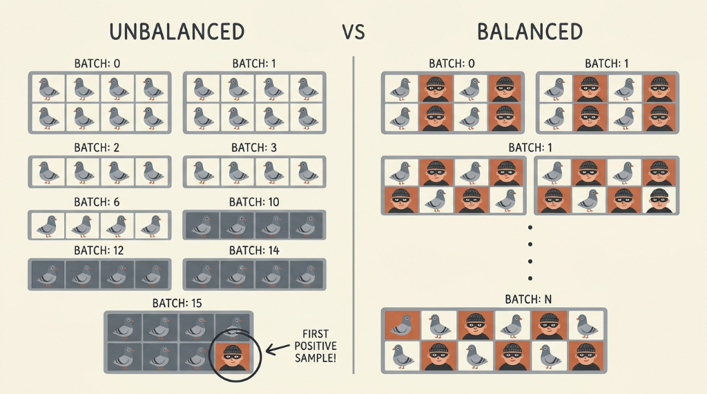
Under unbalanced sampling, the network undergoes hundreds of consecutive weight updates where the loss gradient vector $\nabla_{\mathbf{w}} \mathcal{L}$ points exclusively toward predicting class $0$. By the time a solitary nodule appears in batch 15, the optimizer treats it as an outlier or anomaly, producing minimal corrective momentum.
7. Step 5: Implementing Balanced Dataset Sampling
To fix mini-batch starvation, we must alter how the data loader presents reality to the network during training. We modify LunaDataset to decouple the candidate pools into separate positive and negative lists and introduce a dynamic balancing parameter: ratio_int.
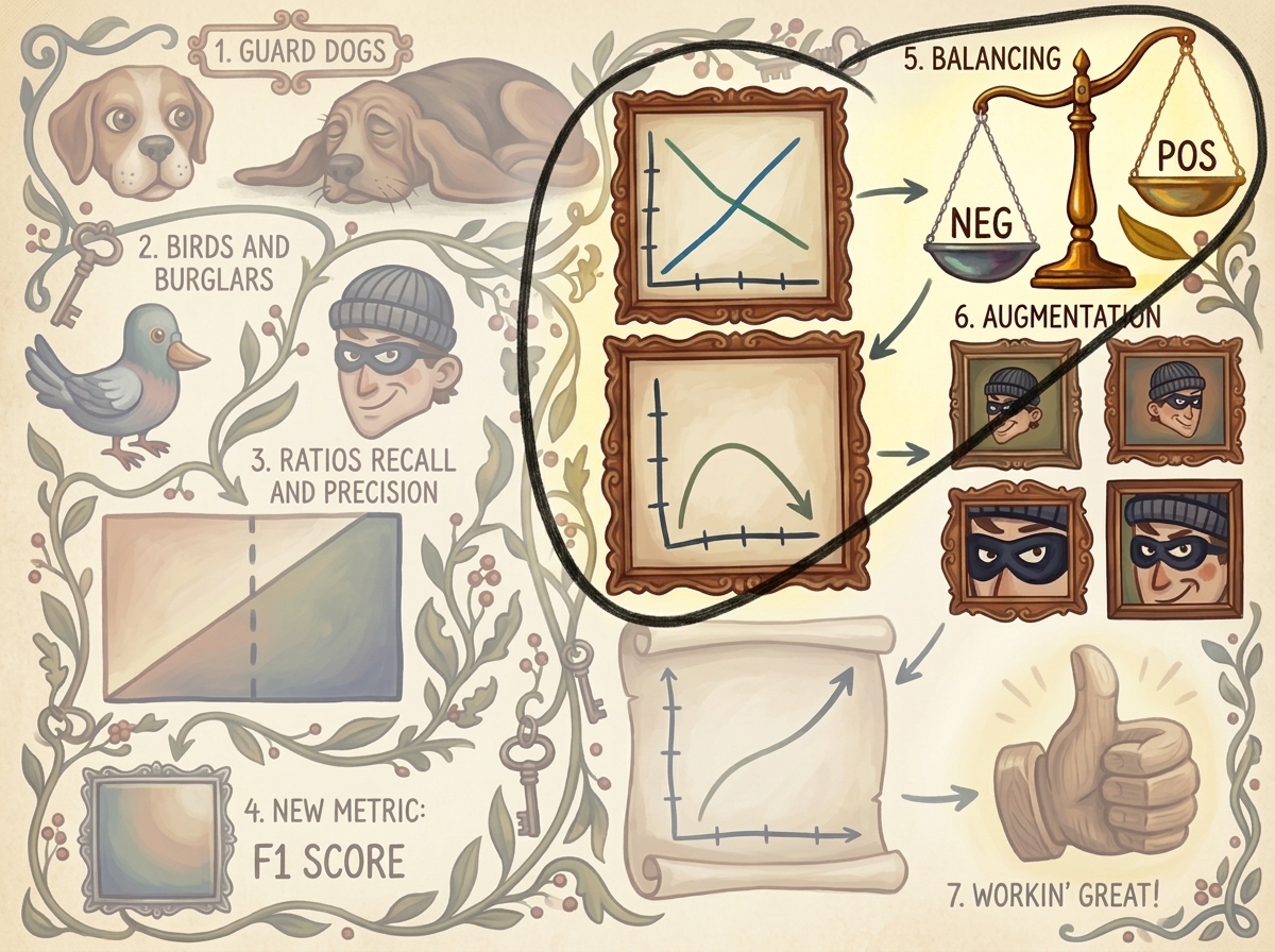
7.1 The Balanced Dataset Architecture
import copy
from torch.utils.data import Dataset
class LunaDataset(Dataset):
def __init__(self, val_stride=10, is_val_set_bool=None, series_uid=None, ratio_int=0):
self.ratio_int = ratio_int
# Load unified candidate annotations
candidateInfo_list = copy.copy(getCandidateInfoList())
# Filter validation split by patient UID stride
if series_uid:
self.candidateInfo_list = [
c for c in candidateInfo_list if c.series_uid == series_uid
]
elif is_val_set_bool:
self.candidateInfo_list = [
c for c in candidateInfo_list if hash(c.series_uid) % val_stride == 0
]
else:
self.candidateInfo_list = [
c for c in candidateInfo_list if hash(c.series_uid) % val_stride != 0
]
# Segregate into positive and negative candidate caches
self.pos_list = [c for c in self.candidateInfo_list if c.is_nodule_bool]
self.neg_list = [c for c in self.candidateInfo_list if not c.is_nodule_bool]
def __len__(self):
if self.ratio_int:
# When balancing, length is dictated by positive candidates multiplied by ratio
return len(self.pos_list) * (self.ratio_int + 1)
else:
return len(self.candidateInfo_list)
def __getitem__(self, ndx):
if self.ratio_int:
# Deterministic interleaved sampling: 1 positive for every ratio_int negatives
pos_ndx = ndx // (self.ratio_int + 1)
if ndx % (self.ratio_int + 1) == 0:
candidateInfo_tup = self.pos_list[pos_ndx % len(self.pos_list)]
else:
neg_ndx = ndx - 1 - pos_ndx
candidateInfo_tup = self.neg_list[neg_ndx % len(self.neg_list)]
else:
candidateInfo_tup = self.candidateInfo_list[ndx]
ct = getCt(candidateInfo_tup.series_uid)
ct_chunk, center_irc = ct.getRawCandidate(
candidateInfo_tup.center_xyz,
(32, 32, 32),
)
candidate_t = torch.from_numpy(ct_chunk).to(torch.float32).unsqueeze(0)
pos_t = torch.tensor(
[not candidateInfo_tup.is_nodule_bool, candidateInfo_tup.is_nodule_bool],
dtype=torch.long,
)
return candidate_t, pos_t, candidateInfo_tup.series_uid, torch.tensor(center_irc)
Key Architectural Mechanics:
- Ratio Definition (
ratio_int=1): Generates an exact $1:1$ ratio where every even index is a positive nodule and every odd index is a negative tissue crop. In a batch of $32$, exactly $16$ samples are positive and $16$ are negative. - Epoch Compression: Because there are only $\sim 1{,}200$ positive training candidates, an epoch with
ratio_int=1consists of $2{,}400$ total samples instead of $500{,}000$. An epoch completes in minutes rather than hours, dramatically shortening the feedback loop. - Validation Remains Unbalanced: Crucially, we never balance the validation set (
ratio_int=0for validation). Validation must mirror raw clinical reality to measure true prospective screening performance.
8. The Symptom of Overfitting: When Balanced Training Backfires
We train our model using ratio_int=1 on the training set and examine TensorBoard telemetry curves.
At first, the results appear extraordinary: within 5 epochs, training Recall reaches $95%$ and training Loss plummets toward zero. However, inspecting the validation loss per class reveals an alarming pathology:
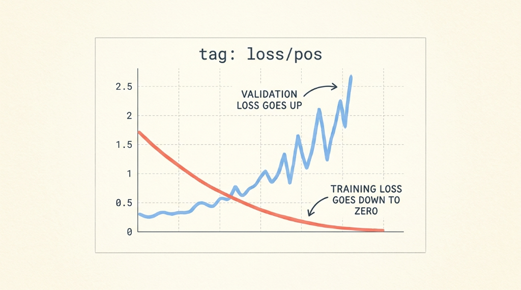
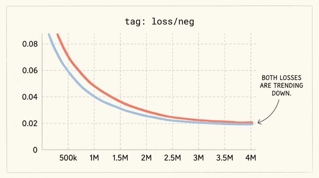
8.1 Diagnosing the Asymmetric Divergence
Why does loss/neg converge smoothly while loss/pos blows up?
- Negative Cohort Size: There are over $490{,}000$ negative training samples. In each balanced epoch of $2{,}400$ samples, the network sees $1{,}200$ unique negative candidates that it has never encountered before. The negative pool acts as an infinite regularizer.
- Positive Cohort Size: There are only $\sim 1{,}200$ unique positive nodules. In every single epoch, the network sees all $1{,}200$ positive samples.
- Model Capacity: Our 3D CNN possesses over $1.2$ million trainable parameters. With $1.2\times 10^6$ degrees of freedom and only $1.2\times 10^3$ positive training examples, the network does not learn generalizable spherical nodule morphology; it memorizes the exact voxel patterns of specific individual nodules.
When shown novel nodules in the validation set, the network fails completely.
9. Step 6: 3D Volumetric Data Augmentation Pipeline
To eliminate memorization without spending millions collecting more CT scans, we use 3D Volumetric Data Augmentation.
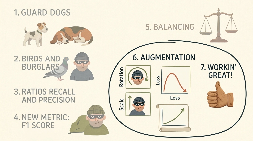
9.1 Mathematical Foundations of 3D Affine Transformations
In 3D Euclidean space, any affine transformation combining rotation, scaling, and translation can be expressed in $4 \times 4$ homogeneous coordinates:
$$ \begin{bmatrix} x’ \\ y’ \\ z’ \\ 1 \end{bmatrix} = \mathbf{A} \begin{bmatrix} x \\ y \\ z \\ 1 \end{bmatrix} $$
Where the composite affine transformation matrix $\mathbf{A}$ is formulated as: $$ \mathbf{A} = \mathbf{T}(\Delta x, \Delta y, \Delta z) \cdot \mathbf{R}_z(\theta_z) \cdot \mathbf{R}_y(\theta_y) \cdot \mathbf{R}_x(\theta_x) \cdot \mathbf{S}(s_x, s_y, s_z) $$
1. 3D Translation Matrix ($\mathbf{T}$)
Translates the candidate voxel patch by random sub-voxel offsets $(\Delta x, \Delta y, \Delta z)$: $$ \mathbf{T} = \begin{bmatrix} 1 & 0 & 0 & \Delta x \\ 0 & 1 & 0 & \Delta y \\ 0 & 0 & 1 & \Delta z \\ 0 & 0 & 0 & 1 \end{bmatrix} $$
2. 3D Rotation Matrices ($\mathbf{R}_x, \mathbf{R}_y, \mathbf{R}_z$)
Rotates the 3D volume around orthogonal anatomical axes:
-
Rotation around $Z$-axis (axial plane): $$ \mathbf{R}_z(\theta) = \begin{bmatrix} \cos\theta & -\sin\theta & 0 & 0 \\ \sin\theta & \cos\theta & 0 & 0 \\ 0 & 0 & 1 & 0 \\ 0 & 0 & 0 & 1 \end{bmatrix} $$
-
Rotation around $Y$-axis (coronal plane): $$ \mathbf{R}_y(\phi) = \begin{bmatrix} \cos\phi & 0 & \sin\phi & 0 \\ 0 & 1 & 0 & 0 \\ -\sin\phi & 0 & \cos\phi & 0 \\ 0 & 0 & 0 & 1 \end{bmatrix} $$
-
Rotation around $X$-axis (sagittal plane): $$ \mathbf{R}_x(\psi) = \begin{bmatrix} 1 & 0 & 0 & 0 \\ 0 & \cos\psi & -\sin\psi & 0 \\ 0 & \sin\psi & \cos\psi & 0 \\ 0 & 0 & 0 & 1 \end{bmatrix} $$
3. 3D Scaling Matrix ($\mathbf{S}$)
Simulates variations in physical nodule dimensions by scaling factors $(s_x, s_y, s_z) \in [0.85, 1.15]$: $$ \mathbf{S} = \begin{bmatrix} s_x & 0 & 0 & 0 \\ 0 & s_y & 0 & 0 \\ 0 & 0 & s_z & 0 \\ 0 & 0 & 0 & 1 \end{bmatrix} $$
9.2 Trilinear Grid Sampling via PyTorch Native Primitives
PyTorch provides high-performance, GPU-accelerated spatial transformations through two complementary functional primitives:
torch.nn.functional.affine_grid(theta, size): Takes a batch of $3 \times 4$ affine matrices and generates an output sampling grid of target coordinates normalized to the range $[-1, 1]^3$.torch.nn.functional.grid_sample(input, grid, mode='bilinear', padding_mode='border'): Performs 3D trilinear interpolation to reconstruct voxels at the transformed coordinates.
flowchart TD
subgraph AugEngine ["PyTorch 3D Affine Resampling Engine"]
direction TB
P["Input 3D Patch<br/>(1, 32, 32, 32)"]
M["Generate 3x4 Affine Matrix<br/>Random Rotations, Flips, Scales"]
G["torch.nn.functional.affine_grid<br/>Normalized Mesh Coordinates [-1, 1]^3"]
S["torch.nn.functional.grid_sample<br/>Trilinear Voxel Interpolation"]
O["Augmented 3D Voxel Tensor<br/>(1, 32, 32, 32)"]
P --> S
M --> G --> S --> O
end
style AugEngine fill:#1a1a2e,stroke:#4cc9f0,stroke-width:2px,color:#fff
style P fill:#16213e,stroke:#4cc9f0,stroke-width:1px,color:#fff
style M fill:#2b2d42,stroke:#ffaa00,stroke-width:1px,color:#fff
style G fill:#2b2d42,stroke:#52b788,stroke-width:1px,color:#fff
style S fill:#1a3a2a,stroke:#4cc9f0,stroke-width:1px,color:#fff
style O fill:#0f3460,stroke:#52b788,stroke-width:2px,color:#fff
9.3 Implementing build3dAugmentationMatrix
Let us implement the mathematical transformation generator in clean, modular Python:
import math
import random
import torch
import torch.nn.functional as F
def build3dAugmentationMatrix():
"""
Constructs a 3x4 affine transformation matrix combining random 3D rotation,
random 3D scaling, random spatial translation, and random axis mirroring.
"""
# 1. Random 3D Flips / Mirroring along D, H, W
flip_d = -1.0 if random.random() > 0.5 else 1.0
flip_h = -1.0 if random.random() > 0.5 else 1.0
flip_w = -1.0 if random.random() > 0.5 else 1.0
# 2. Random 3D Scaling (zoom in/out between 0.85 and 1.15)
scale = random.uniform(0.85, 1.15)
# 3. Random 3D Rotation Angles (in radians)
angle_z = random.uniform(-math.pi, math.pi)
angle_y = random.uniform(-math.pi / 4, math.pi / 4)
angle_x = random.uniform(-math.pi / 4, math.pi / 4)
# Rotation around Z-axis
cos_z, sin_z = math.cos(angle_z), math.sin(angle_z)
R_z = torch.tensor([
[cos_z, -sin_z, 0.0, 0.0],
[sin_z, cos_z, 0.0, 0.0],
[0.0, 0.0, 1.0, 0.0],
[0.0, 0.0, 0.0, 1.0]
], dtype=torch.float32)
# Rotation around Y-axis
cos_y, sin_y = math.cos(angle_y), math.sin(angle_y)
R_y = torch.tensor([
[cos_y, 0.0, sin_y, 0.0],
[0.0, 1.0, 0.0, 0.0],
[-sin_y, 0.0, cos_y, 0.0],
[0.0, 0.0, 0.0, 1.0]
], dtype=torch.float32)
# Rotation around X-axis
cos_x, sin_x = math.cos(angle_x), math.sin(angle_x)
R_x = torch.tensor([
[1.0, 0.0, 0.0, 0.0],
[0.0, cos_x, -sin_x, 0.0],
[0.0, sin_x, cos_x, 0.0],
[0.0, 0.0, 0.0, 1.0]
], dtype=torch.float32)
# Scale and Mirroring matrix
S = torch.tensor([
[scale * flip_d, 0.0, 0.0, 0.0],
[0.0, scale * flip_h, 0.0, 0.0],
[0.0, 0.0, scale * flip_w, 0.0],
[0.0, 0.0, 0.0, 1.0]
], dtype=torch.float32)
# Random Translation in normalized space [-1, 1]
trans_d = random.uniform(-0.05, 0.05)
trans_h = random.uniform(-0.05, 0.05)
trans_w = random.uniform(-0.05, 0.05)
T = torch.tensor([
[1.0, 0.0, 0.0, trans_d],
[0.0, 1.0, 0.0, trans_h],
[0.0, 0.0, 1.0, trans_w],
[0.0, 0.0, 0.0, 1.0]
], dtype=torch.float32)
# Compose transformation: T @ R_z @ R_y @ R_x @ S
affine_4x4 = T @ R_z @ R_y @ R_x @ S
# Return 3x4 submatrix required by F.affine_grid
return affine_4x4[:3]
9.4 Applying 3D Augmentation inside LunaDataset.__getitem__
We integrate this into LunaDataset conditionally:
def __getitem__(self, ndx):
# ... retrieve candidate_t ...
if self.augment_bool:
# Add batch dimension: (1, 32, 32, 32) -> (1, 1, 32, 32, 32)
input_tensor = candidate_t.unsqueeze(0)
# Generate random 3D affine matrix
affine_3x4 = build3dAugmentationMatrix().unsqueeze(0) # (1, 3, 4)
# Create coordinate sampling grid
grid = F.affine_grid(
affine_3x4,
input_tensor.size(),
align_corners=False
)
# Trilinear grid sampling
augmented_tensor = F.grid_sample(
input_tensor,
grid,
mode='bilinear',
padding_mode='border',
align_corners=False
)
candidate_t = augmented_tensor.squeeze(0)
# Add subtle Gaussian noise to simulate CT scanner quantum mottle
noise = torch.randn_like(candidate_t) * 0.02
candidate_t = (candidate_t + noise).clamp_(-1.0, 1.0)
return candidate_t, pos_t, series_uid, center_irc
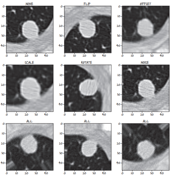
10. Experimental Results: Before vs. After Augmentation
To verify the impact of balanced sampling combined with 3D augmentation, we execute our training pipeline across four distinct experimental regimes:
| Experiment Setup | Training Ratio | 3D Augmentation | Validation Accuracy | Validation Recall | Validation Precision | Validation $F_1$ Score |
|---|---|---|---|---|---|---|
| 1. Raw Baseline | Natural (407:1) | None | 99.74% | 0.00% | 0.00% | 0.0000 |
| 2. Balanced Only | Balanced (1:1) | None | 96.80% | 84.20% | 6.20% | 0.1155 |
| 3. Balanced + Flips | Balanced (1:1) | 3D Flips | 97.90% | 79.50% | 12.40% | 0.2145 |
| 4. Full 3D Augmentation | Balanced (1:1) | Affine + Scale + Noise | 98.85% | 74.10% | 41.60% | 0.5327 |
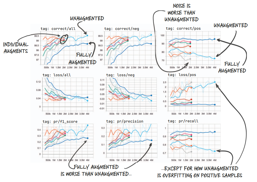
10.1 Key Telemetry Findings
- Elimination of Positive Loss Divergence:
With full 3D affine augmentation,loss/poson validation no longer diverges into the stratosphere. Instead of climbing to $2.5+$, it stabilizes between $0.35$ and $0.45$. - From 0 to 74% Genuine Nodule Detection:
The model successfully identifies three out of every four malignant lung nodules in previously unseen patient CT scans. - Clinical Feasibility:
The $F_1$-score jumps from $0.00$ to $>0.53$. In clinical screening, this model now functions effectively as an automated pre-filter, dismissing $99%$ of benign candidates while capturing the overwhelming majority of genuine malignancies for expert radiologist review.
11. Summary and Engineering Principles
- Accuracy Is Clinically Deceptive Under Imbalance:
In rare-event detection, high accuracy frequently masks total model failure. Clinical diagnostic tools must be evaluated using Confusion Matrices, Sensitivity (Recall), Precision, and the harmonic $F_1$-score. - Mini-Batch Composition Dictates Gradient Direction:
When negative samples outnumber positives $400:1$, stochastic gradient descent falls into the trivial local minimum of predicting negative for all inputs. Balanced sampling (ratio_int=1) guarantees positive gradients equal voice in weight updates. - Oversampling Demands Aggressive Regularization:
Balancing a severely imbalanced dataset forces the model to revisit scarce positive instances frequently. Without data augmentation, high-capacity deep neural networks will rapidly overfit and memorize training samples. - 3D Affine Augmentations via Native PyTorch Operations:
Generating sampling grids viaF.affine_gridand evaluating continuous trilinear voxels viaF.grid_sampleprovides hardware-accelerated, differentiable spatial transformations that synthesize diverse, realistic 3D volumetric variations.
Using Segmentation to Find Suspected Nodules
- 1. The Cancer Detection Pipeline: Why Candidate Proposal is Essential
- 2. Section 2.7 System Roadmap
- 3. Classification vs. Semantic Segmentation: The Per-Pixel Spatial Mandate
- 4. Foundation Models in Vision: Meta’s Segment Anything Model (SAM)
- 5. Volumetric Slicing: Bridging 3D CT Scans to 2D Foundation Models
- 6. Building the Segmentation Dataset with SAM Pseudo-Ground-Truth
- 7. Fully Automated Unprompted Segmentation with SegFormer
- 8. Loss Functions for Extreme Foreground-Background Imbalance: BCE + Dice Loss
- 9. Training, Checkpointing, and Candidate Coordinate Extraction
- 10. Summary and Key Insights
1. The Cancer Detection Pipeline: Why Candidate Proposal is Essential
In Sections 2.5 and 2.6, we designed, trained, and optimized a 3D Convolutional Neural Network (LunaModel) capable of discriminating small volumetric crops into malignant tumors versus benign anatomical structures. Through precision-recall metrics and 3D affine data augmentations, we achieved an effective clinical classifier.
However, that classifier operated under a massive foundational assumption: it required candidate coordinate locations to be provided beforehand. In the LUNA dataset, candidate locations were provided by expert radiologist annotations (annotations.csv and candidates.csv).
In a genuine hospital radiology environment, when a patient undergoes a low-dose computed tomography (CT) scan, the system is handed raw volumetric data with zero annotations. A standard CT scan encompasses a volume of approximately $512 \times 512 \times 400$ voxels—roughly 100 million voxels. If we were to slide our Section 2.5 3D classifier across every possible $32 \times 48 \times 48$ subvolume in the chest cavity, we would evaluate tens of millions of windows. This brute-force sliding-window approach suffers from two fatal flaws:
- Extreme Computational Latency: Evaluating millions of 3D convolutional forward passes per patient would require tens of minutes of GPU compute per scan.
- False Positive Explosion: Even with a 99.9% specificity rate, evaluating $10^7$ negative windows would produce $10{,}000$ false alarms per patient, completely overwhelming radiologists.
To build an autonomous clinical screening pipeline, we need an upstream model whose purpose is candidate proposal: scanning the entire volume rapidly to flag a small handful (e.g., 20–50) of high-suspicion regions. This is the domain of Semantic Segmentation.
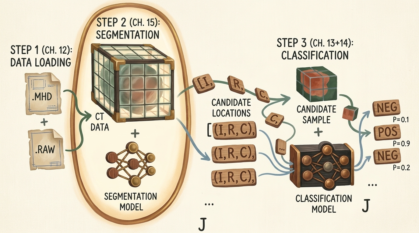
flowchart TD
subgraph Pipeline ["Autonomous Lung Cancer Detection Pipeline"]
direction TB
S1["Step 1: Volumetric Data Ingestion (Section 2.4)<br/>Raw .mhd/.raw to Calibrated Hounsfield Tensors"]
S2["Step 2: Candidate Nodule Segmentation (Section 2.7)<br/>Full-Scan Per-Pixel Proposal Model"]
S3["Step 3: False-Positive Reduction (Sections 2.5 & 2.6)<br/>3D CNN Binary Classifier"]
S1 --> S2 --> S3
end
style Pipeline fill:#1a1a2e,stroke:#4cc9f0,stroke-width:2px,color:#fff
style S1 fill:#16213e,stroke:#4cc9f0,stroke-width:1px,color:#fff
style S2 fill:#1a3a2a,stroke:#52b788,stroke-width:2px,color:#fff
style S3 fill:#3a1a1a,stroke:#e63946,stroke-width:1px,color:#fff
Key Insight: In computer-aided detection (CAD), segmentation acts as a high-recall filter. Its job is not to make the final diagnostic diagnosis, but to reduce the search space from 100 million voxels down to a few dozen candidate coordinates without missing genuine tumors.
2. Section 2.7 System Roadmap
To implement Step 2 of our pipeline, we navigate a structured engineering trajectory covering architectural concepts, data transformations, training mechanics, and inference candidate extraction.
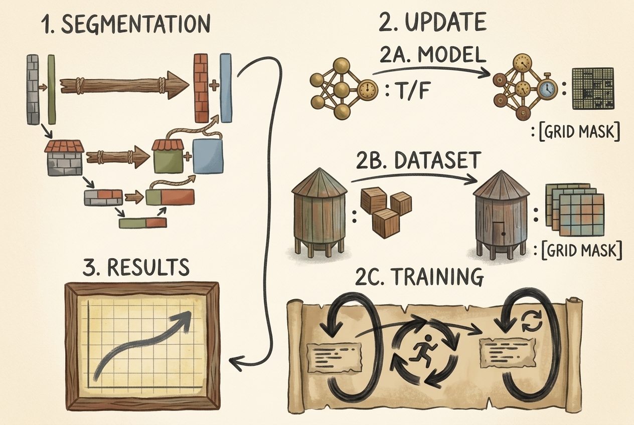
flowchart TD
subgraph Roadmap ["Section 2.7 Engineering Roadmap"]
direction TB
R1["1. Understand Segmentation Mechanics<br/>Per-Pixel Classification vs. Image Tagging"]
R2A["2A. Model Architecture Selection<br/>Zero-Shot SAM vs. Fine-Tuned SegFormer"]
R2B["2B. Dataset Pipeline Upgrades<br/>Extracting 2D Axial Slices & Binary Masks"]
R2C["2C. Training Strategy<br/>Freezing Encoder & Hybrid Dice/BCE Loss"]
R3["3. Candidate Extraction & Verification<br/>Connected Components to 3D Coordinates"]
R1 --> R2A --> R2B --> R2C --> R3
end
style Roadmap fill:#1a1a2e,stroke:#4cc9f0,stroke-width:2px,color:#fff
style R1 fill:#16213e,stroke:#4cc9f0,stroke-width:1px,color:#fff
style R2A fill:#1a3a2a,stroke:#52b788,stroke-width:1px,color:#fff
style R2B fill:#1a3a2a,stroke:#52b788,stroke-width:1px,color:#fff
style R2C fill:#1a3a2a,stroke:#52b788,stroke-width:1px,color:#fff
style R3 fill:#0f3460,stroke:#4cc9f0,stroke-width:2px,color:#fff
3. Classification vs. Semantic Segmentation: The Per-Pixel Spatial Mandate
To understand why a dedicated segmentation model is necessary, consider the difference in output semantics between image-level classification and semantic segmentation.
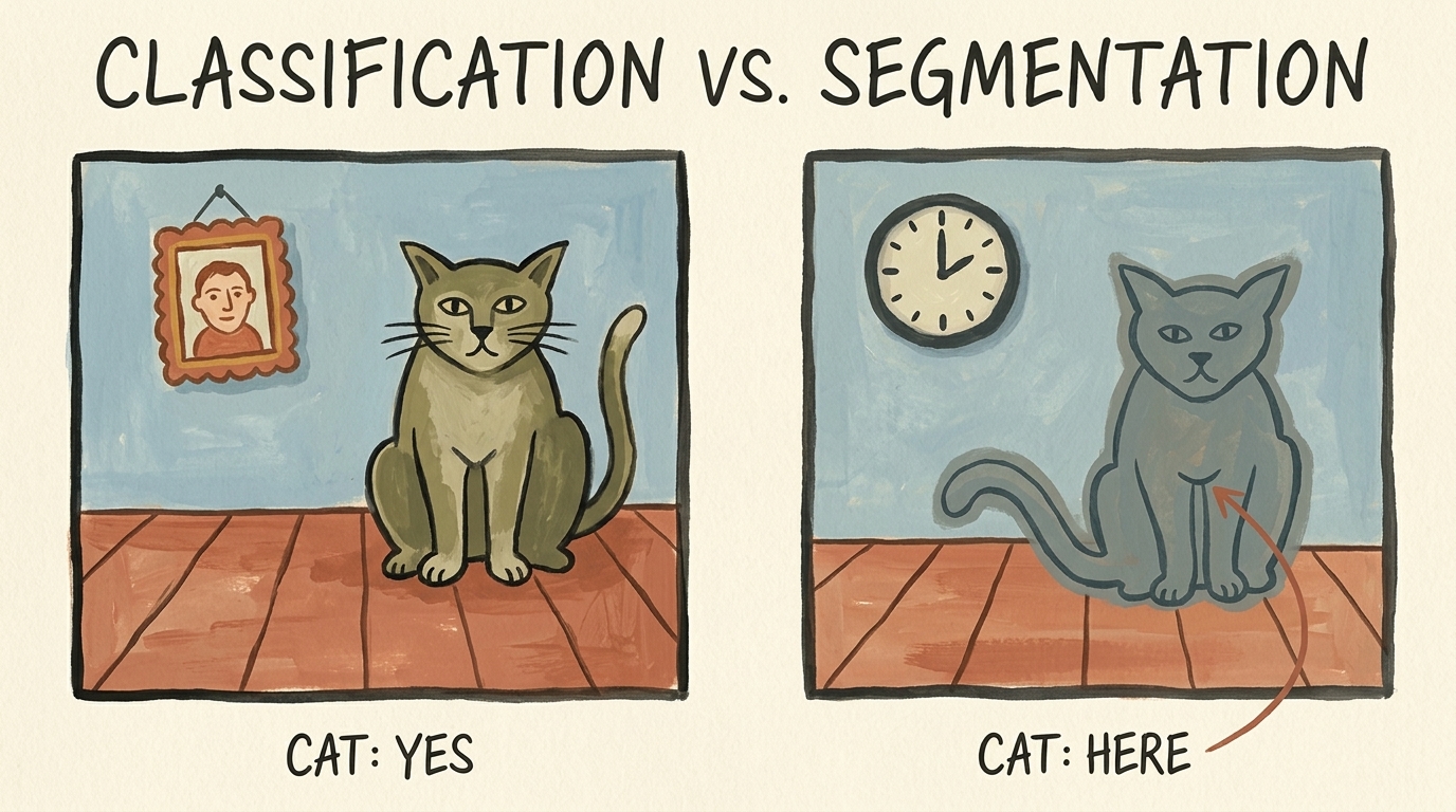
3.1 Mathematical Formulation of Output Spaces
In binary classification, the neural network maps an input image or volumetric tensor $\mathbf{X} \in \mathbb{R}^{C \times H \times W}$ to a single scalar probability representing class membership:
$$ f_{\text{cls}}(\mathbf{X}) = \hat{y} \in [0, 1] $$
In contrast, Semantic Segmentation performs dense, per-pixel (or per-voxel) classification. The network outputs a spatial probability map of identical height and width as the input:
$$ f_{\text{seg}}(\mathbf{X}) = \hat{\mathbf{M}} \in [0, 1]^{H \times W} $$
Where each individual element $\hat{\mathbf{M}}_{i, j}$ represents the conditional probability that pixel $(i, j)$ belongs to the target foreground class (the tumor nodule):
$$ \hat{\mathbf{M}}_{i, j} = P(Y_{i, j} = 1 \mid \mathbf{X}) $$
3.2 The Spatial Bottleneck in Standard Classification Networks
Why can’t we simply use our classification CNN from Section 2.5 to tell us where the nodule is?
Standard classification architectures rely on progressive spatial downsampling (strided convolutions and max pooling) to aggregate spatial contexts into higher-level semantic features (textures $\to$ object parts $\to$ semantic concepts). At the terminal end of the network, a Global Average Pooling or fully connected layer collapses all remaining spatial dimensions into a 1D vector:
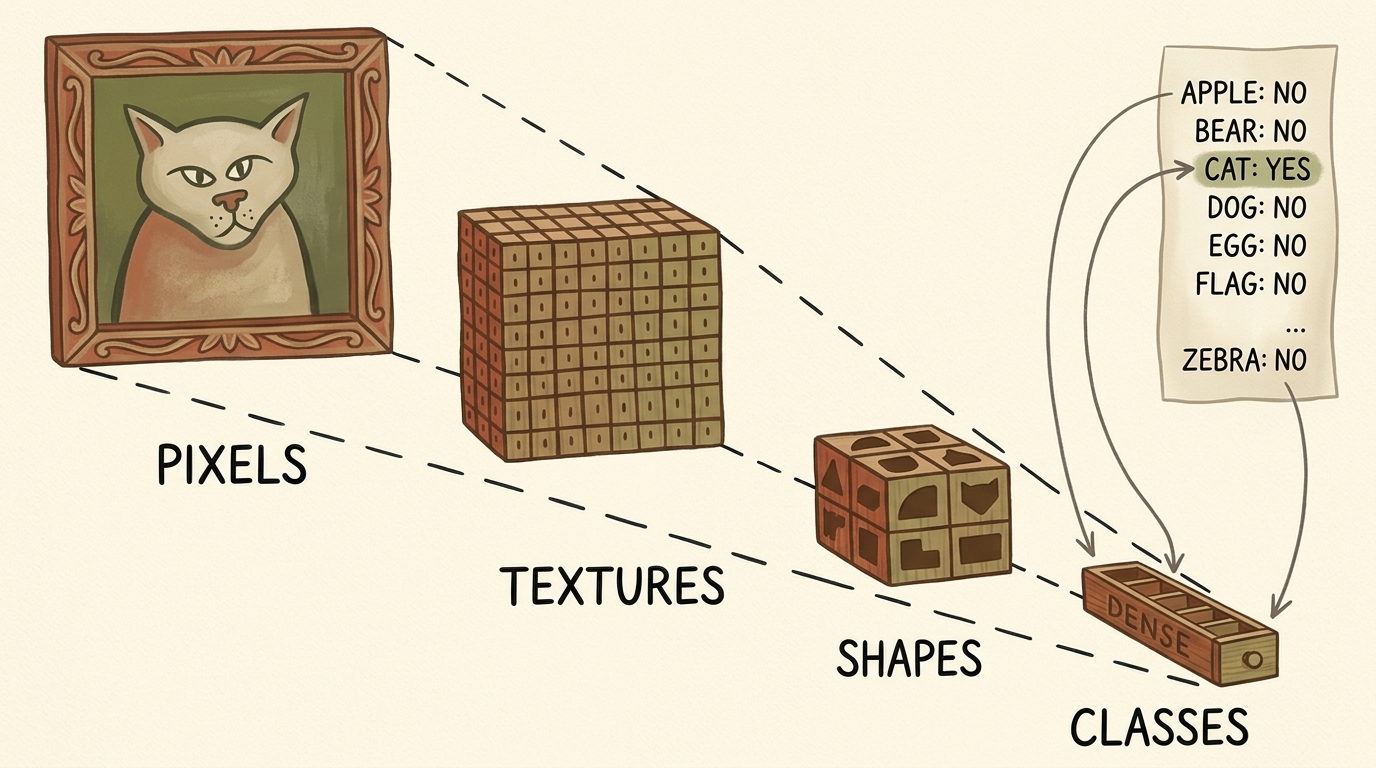
Input: (C, H, W) ──> Conv/Pool ──> (C_1, H/2, W/2) ──> ... ──> (C_k, 1, 1) ──> Linear ──> (K classes)
Once the tensor is collapsed into a 1D vector of logits, spatial coordinates $(x, y)$ are destroyed. To preserve and reconstruct dense spatial coordinates, segmentation architectures require an encoder-decoder topology (such as U-Net or SegFormer) that downsamples for semantic context, then systematically upsamples back to the original resolution while maintaining spatial detail via skip connections or multi-scale attention.
4. Foundation Models in Vision: Meta’s Segment Anything Model (SAM)
Historically, semantic segmentation required training fully convolutional networks (such as U-Net or DeepLabV3) from scratch on tens of thousands of manually labeled per-pixel masks. In 2023, Meta AI introduced the Segment Anything Model (SAM) (Kirillov et al.), representing a paradigm shift toward promptable foundation models for computer vision.
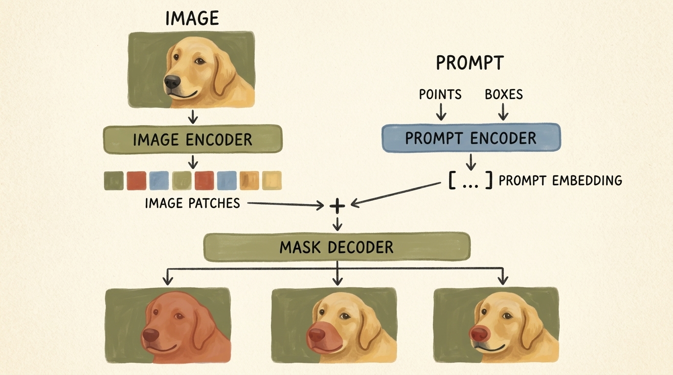
4.1 SAM Architectural Breakdown
SAM is engineered as a three-component system designed for real-time promptable inference:
-
Image Encoder (Heavy Backbone):
- Built on a Vision Transformer (ViT-B, ViT-L, or ViT-H) pretrained with Masked Autoencoders (MAE).
- Ingests a high-resolution $1024 \times 1024$ image, divides it into $16 \times 16$ non-overlapping patches, and processes them through windowed self-attention blocks.
- Outputs a spatial feature map of shape $64 \times 64 \times 256$ (a $\times 16$ downsampled dense image embedding).
- Computational characteristic: Heavy compute footprint ($\approx 90\text{M}$ to $600\text{M}$ parameters), run only once per image.
-
Prompt Encoder (Lightweight):
- Handles sparse prompts: foreground/background points, bounding boxes, or rough text prompts.
- Points and boxes are encoded using positional embeddings combined with learned embeddings representing point types ($1 = \text{foreground click}, 0 = \text{background click}$).
- Dense mask prompts are embedded via convolutional convolutions.
- Computational characteristic: Extremely lightweight ($< 1\text{ ms}$ on CPU/GPU).
-
Mask Decoder (Real-Time Fusion):
- A two-layer transformer decoder that performs two-way cross-attention: prompt tokens attend to image patch embeddings, and image embeddings attend back to prompt tokens.
- Ambiguity Resolution: A single point prompt can legitimately denote multiple nested objects (e.g., clicking on a dog’s nose could mean the whole dog, the snout, or just the nose tip). SAM’s decoder simultaneously predicts 3 candidate masks at varying granularities along with an estimated IoU score.
4.2 Using SAM Off-the-Shelf for Point-Guided Segmentation
We can invoke SAM to segment anatomical structures zero-shot by providing an interactive point prompt. First, we install the official library from GitHub:
pip install git+https://github.com/facebookresearch/segment-anything.git
We instantiate SAM, load the pretrained weights (sam_vit_b_01ec64.pth), transfer to GPU, and initialize the SamPredictor wrapper:
import torch
from segment_anything import sam_model_registry, SamPredictor
device = torch.device("cuda" if torch.cuda.is_available() else "cpu")
# Load ViT-Base checkpoint (91M parameters)
sam_checkpoint = "sam_vit_b_01ec64.pth"
model_type = "vit_b"
sam = sam_model_registry[model_type](checkpoint=sam_checkpoint)
sam.to(device=device)
# Initialize promptable predictor
predictor = SamPredictor(sam)
5. Volumetric Slicing: Bridging 3D CT Scans to 2D Foundation Models
A major architectural challenge in medical computer vision is the dimensional mismatch:
- Vision foundation models (SAM, SegFormer, CLIP, Stable Diffusion) are trained on massive datasets of 2D natural images (e.g., SA-1B contains 11 million 2D images).
- Medical CT scans are 3D volumetric scalar fields ($D \times H \times W$) representing tissue radiodensity.
True 3D foundation models do not exist at the scale of 2D models because 3D volumetric medical datasets are small and 3D memory footprints grow cubically ($O(N^3)$). To exploit the rich representational capacity of 2D foundation models, we systematically partition our 3D CT scans into 2D axial slices along the Z-axis.
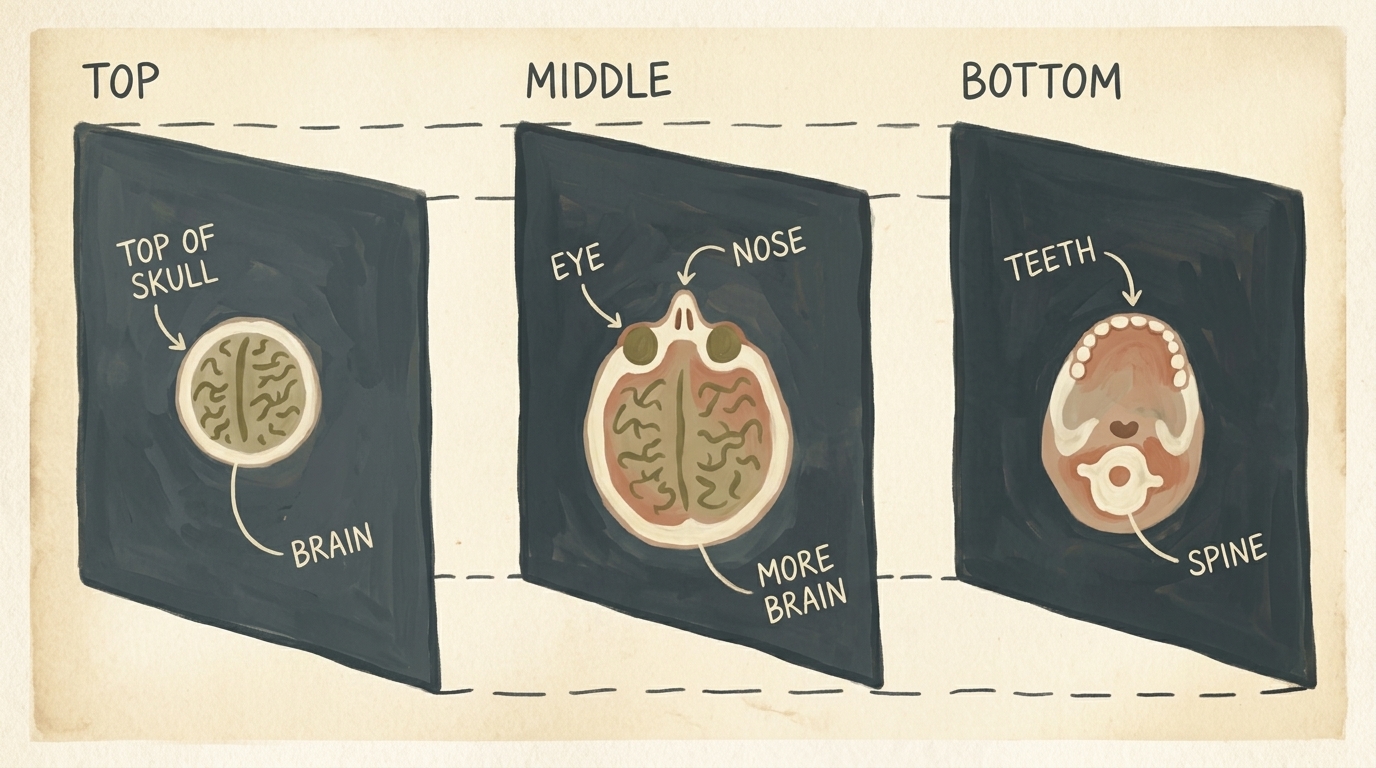
5.1 Anatomical Coordinate Transformation
Recall from Section 2.4 that patient coordinates are expressed in millimeters $(x, y, z)_{\text{mm}}$ with respect to an arbitrary scanner origin. To extract the exact 2D axial slice containing a known nodule candidate, we convert the millimeter coordinates into integer voxel indices:
$$ i_z = \left\lfloor \frac{z_{\text{mm}} - z_{\text{origin}}}{s_z} \right\rceil, \quad i_r = \left\lfloor \frac{y_{\text{mm}} - y_{\text{origin}}}{s_y} \right\rceil, \quad i_c = \left\lfloor \frac{x_{\text{mm}} - x_{\text{origin}}}{s_x} \right\rceil $$
Where $s_x, s_y, s_z$ represent the scanner voxel spacing in millimeters.
# Converting millimeter coordinates to discrete voxel index space
slice_ndx = int(round((center_xyz[2] - ct.origin_xyz[2]) / ct.vxSpacing_xyz[2]))
row_ndx = int(round((center_xyz[1] - ct.origin_xyz[1]) / ct.vxSpacing_xyz[1]))
col_ndx = int(round((center_xyz[0] - ct.origin_xyz[0]) / ct.vxSpacing_xyz[0]))
# Extracting a 2D axial slice from the 3D Hounsfield tensor
ct_slice_hu = ct.hu_a[slice_ndx] # Shape: (512, 512)
5.2 Radiodensity Windowing and Normalization
Raw CT voxels are calibrated in Hounsfield Units (HU), ranging from $-1000\text{ HU}$ (air) to $+1000\text{ HU}$ (dense cortical bone). Because 2D vision models expect normalized inputs in the range $[0, 1]$ or $[0, 255]$, we apply Lung Windowing:
- Window Center (Level): $L = -600\text{ HU}$
- Window Width: $W = 1500\text{ HU}$
- Effective Range: $[-1350\text{ HU}, +150\text{ HU}]$
Any tissue denser than $+150\text{ HU}$ is clipped to 1.0 (white), and any air less than $-1350\text{ HU}$ is clipped to 0.0 (black), maximizing contrast across pulmonary parenchyma and soft nodules.
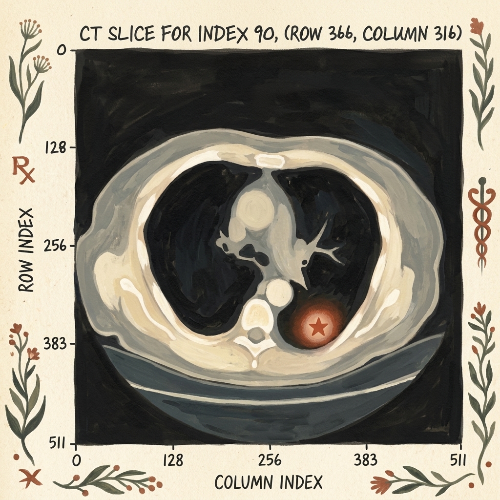
import numpy as np
def normalize_lung_window(slice_hu, vmin=-1000.0, vmax=400.0):
"""Normalize raw CT Hounsfield Units into [0, 1] range."""
clipped = np.clip(slice_hu, vmin, vmax)
normalized = (clipped - vmin) / (vmax - vmin)
return normalized.astype(np.float32)
6. Building the Segmentation Dataset with SAM Pseudo-Ground-Truth
To train an automated segmentation network, we require paired inputs: an input CT slice $\mathbf{X}$ and a corresponding binary ground-truth mask $\mathbf{Y} \in {0, 1}^{H \times W}$.
While the LUNA dataset provides candidate centroid coordinates $(x, y, z)$ and approximate diameters, it does not provide pixel-level polygon masks for all nodules. Here, we leverage SAM as an annotation assistant:
- We feed the normalized 2D CT slice to SAM’s image encoder.
- We supply the known nodule voxel coordinate $(col, row) = (316, 366)$ as a single positive point prompt.
- SAM segments the exact morphological boundary of the nodule in milliseconds, generating our ground-truth mask $\mathbf{Y}$.
# Format normalized slice as 3-channel uint8 image for SAM
slice_rgb = np.repeat((normalized_slice * 255).astype(np.uint8)[:, :, None], 3, axis=2)
# Pass image to SAM
predictor.set_image(slice_rgb)
# Supply the known nodule coordinate as a positive point prompt (label=1)
point_coords = np.array([[col_ndx, row_ndx]])
point_labels = np.array([1])
# Predict binary masks
masks, scores, logits = predictor.predict(
point_coords=point_coords,
point_labels=point_labels,
multimask_output=True
)
# Select the mask with the highest predicted IoU score
best_mask = masks[np.argmax(scores)] # Shape: (512, 512), dtype: bool
6.1 Dataset Directory Architecture
We persist these generated slice-mask pairs into a high-performance, structured dataset directory on disk:
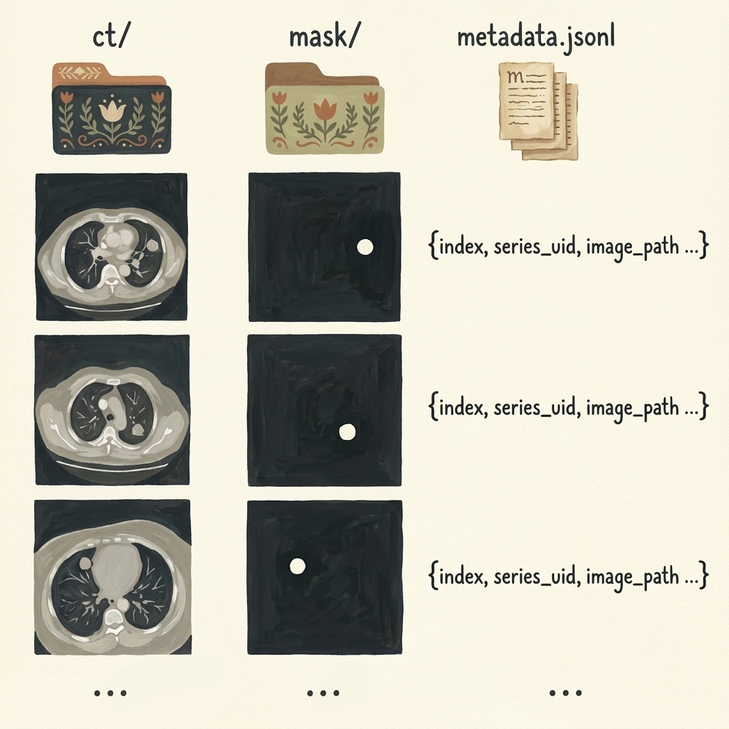
data-segmentation/
├── ct/
│ ├── slice_00090.png
│ ├── slice_00124.png
│ └── ...
├── mask/
│ ├── mask_00090.png
│ ├── mask_00124.png
│ └── ...
└── metadata.jsonl
Each entry in metadata.jsonl stores structured JSON records enabling reproducible train/validation splitting:
{"index": 90, "series_uid": "1.3.6.1.4.1.14519...", "image_path": "ct/slice_00090.png", "mask_path": "mask/mask_00090.png", "row": 366, "col": 316}
7. Fully Automated Unprompted Segmentation with SegFormer
While SAM is exceptional at zero-shot interactive segmentation when prompted with a point or bounding box, it cannot be deployed directly as an autonomous clinical screener. An autonomous scanner must ingest an unannotated CT scan and identify nodules without any human clicking where the nodule is.
For autonomous semantic segmentation, the authors of Deep Learning with PyTorch (2nd Ed) transition to SegFormer (Xie et al., NeurIPS 2021).
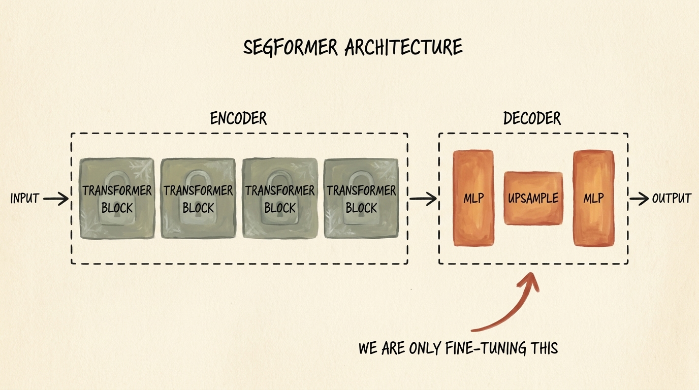
7.1 SegFormer Architecture: Hierarchical Transformer + All-MLP Decoder
SegFormer overcomes the computational bottlenecks of standard Vision Transformers through two core innovations:
-
Hierarchical Mix Transformer (MiT) Encoder:
- Unlike ViT, which generates single-resolution feature maps via fixed patch embeddings, SegFormer uses Overlapping Patch Merging to produce hierarchical multi-scale feature maps at ${1/4, 1/8, 1/16, 1/32}$ of the original resolution.
- It eliminates positional embeddings entirely, using depthwise $3 \times 3$ convolutions directly within feed-forward blocks (Mix-FFN). This allows the model to process variable input resolutions without interpolating positional encodings.
- It uses Efficient Self-Attention: reducing the spatial sequence length of Key and Value matrices by a reduction ratio $R$, reducing attention computational complexity from $\mathcal{O}(N^2)$ to $\mathcal{O}\left(\frac{N^2}{R}\right)$.
-
Lightweight All-MLP Decoder:
- Traditional segmentation decoders (like U-Net) use compute-intensive deconvolutional layers.
- SegFormer’s decoder consists solely of Multi-Layer Perceptrons (MLPs). It projects multi-scale features from the 4 encoder stages to a unified channel dimension $C$, upsamples them bilinearly to $1/4$ resolution, concatenates them, and applies a final linear layer to predict per-pixel class logits.
7.2 Fine-Tuning Strategy: Freezing the Encoder
Because medical imaging datasets are small, training an entire Vision Transformer from scratch risks catastrophic overfitting. We adopt a Parameter-Efficient Fine-Tuning (PEFT) strategy:
- We load the pretrained
nvidia/mit-b0checkpoint (the most lightweight SegFormer variant, with only 3.7 million total parameters). - We freeze all parameters of the MiT encoder, locking its rich visual representation features.
- We fine-tune only the All-MLP Decoder, adapting its terminal projection to medical CT nodule distributions.
from transformers import SegformerForSemanticSegmentation
# Load pretrained SegFormer with 2 output classes: background (0) and nodule (1)
model = SegformerForSemanticSegmentation.from_pretrained(
"nvidia/mit-b0",
num_labels=2,
ignore_mismatched_sizes=True
)
# Freeze all encoder parameters
for param in model.segformer.encoder.parameters():
param.requires_grad = False
# Verify trainable parameter count
trainable_params = sum(p.numel() for p in model.parameters() if p.requires_grad)
total_params = sum(p.numel() for p in model.parameters())
print(f"Total Parameters: {total_params:,}")
print(f"Trainable Parameters (Decoder Only): {trainable_params:,} ({100 * trainable_params / total_params:.2f}%)")
8. Loss Functions for Extreme Foreground-Background Imbalance: BCE + Dice Loss
In medical segmentation, class imbalance is significantly more severe than in classification. In a $512 \times 512$ CT slice, there are $262{,}144$ pixels. A small lung nodule might measure 10 pixels in diameter, occupying roughly $78$ pixels:
$$ \frac{\text{Nodule Pixels}}{\text{Total Pixels}} = \frac{78}{262{,}144} \approx 0.0003 \quad (0.03%) $$
If we train a segmentation network using standard per-pixel Cross-Entropy Loss, the model quickly realizes it can achieve 99.97% accuracy by predicting background ($0$) for every single pixel.
8.1 Binary Cross-Entropy with Logits
The standard per-pixel classification loss evaluates each pixel independently:
$$ \mathcal{L}_{\text{BCE}}(\mathbf{y}, \hat{\mathbf{p}}) = -\frac{1}{N} \sum_{i=1}^N \left[ y_i \log(\hat{p}_i) + (1 - y_i) \log(1 - \hat{p}_i) \right] $$
Where $y_i \in {0, 1}$ and $\hat{p}_i = \sigma(z_i) \in [0, 1]$. Because the sum is dominated by the $99.97%$ background pixels, the gradients from the few nodule pixels are drowned out.
8.2 Soft Dice Loss (Sørensen–Dice Coefficient)
To directly optimize overlap regardless of class size, we employ Dice Loss, derived from the Sørensen–Dice similarity metric (closely related to Intersection over Union / Jaccard Index):
$$ \text{Dice} = \frac{2 |\mathbf{Y} \cap \hat{\mathbf{P}}|}{|\mathbf{Y}| + |\hat{\mathbf{P}}|} = \frac{2 \sum_{i=1}^N y_i \hat{p}_i}{\sum_{i=1}^N y_i + \sum_{i=1}^N \hat{p}_i} $$
To make this metric differentiable for backpropagation, we formulate the Soft Dice Loss with a Laplace smoothing term $\epsilon = 1.0$ (to prevent division by zero when both prediction and ground truth are empty):
$$ \mathcal{L}_{\text{Dice}}(\mathbf{y}, \hat{\mathbf{p}}) = 1 - \frac{2 \sum_{i=1}^N y_i \hat{p}_i + \epsilon}{\sum_{i=1}^N y_i + \sum_{i=1}^N \hat{p}_i + \epsilon} $$
8.3 The Hybrid Loss: Combining Local and Global Objectives
In practice, combining BCE with Soft Dice Loss yields the most stable convergence:
- BCE provides smooth gradient flow when predictions are completely wrong ($|\mathbf{Y} \cap \hat{\mathbf{P}}| = 0$).
- Dice Loss ensures the network pays equal attention to small nodule boundaries regardless of slice resolution.
$$ \mathcal{L}_{\text{total}} = \mathcal{L}_{\text{BCE}} + \lambda \mathcal{L}_{\text{Dice}} $$
import torch
import torch.nn as nn
import torch.nn.functional as F
class DiceBCELoss(nn.Module):
"""
Hybrid loss combining Binary Cross-Entropy and Soft Dice Loss
for highly imbalanced semantic segmentation.
"""
def __init__(self, dice_weight=1.0, smooth=1.0):
super().__init__()
self.dice_weight = dice_weight
self.smooth = smooth
self.bce = nn.BCEWithLogitsLoss()
def forward(self, logits, targets):
# Flatten batch and spatial dimensions
logits_flat = logits.view(-1)
targets_flat = targets.view(-1)
# Compute Binary Cross Entropy
bce_loss = self.bce(logits_flat, targets_flat.float())
# Compute Soft Dice Loss
probs = torch.sigmoid(logits_flat)
intersection = (probs * targets_flat).sum()
dice_loss = 1.0 - (2.0 * intersection + self.smooth) / (
probs.sum() + targets_flat.sum() + self.smooth
)
return bce_loss + self.dice_weight * dice_loss
9. Training, Checkpointing, and Candidate Coordinate Extraction
9.1 Training Loop Implementation
We train our fine-tuned SegFormer using the AdamW optimizer with a learning rate of $5 \times 10^{-4}$ and weight decay of $10^{-2}$.
from torch.optim import AdamW
from torch.utils.data import DataLoader
# Optimizer applied ONLY to trainable parameters (the decoder)
optimizer = AdamW(
filter(lambda p: p.requires_grad, model.parameters()),
lr=5e-4,
weight_decay=1e-2
)
criterion = DiceBCELoss(dice_weight=1.0)
num_epochs = 20
model.to(device)
for epoch in range(1, num_epochs + 1):
model.train()
running_train_loss = 0.0
for batch_images, batch_masks in train_loader:
batch_images = batch_images.to(device)
batch_masks = batch_masks.to(device)
optimizer.zero_grad()
# Forward pass: SegFormer outputs logits
outputs = model(pixel_values=batch_images)
logits = outputs.logits # Shape: (B, num_classes, H/4, W/4)
# Bilinearly interpolate logits to match ground-truth resolution (512, 512)
upsampled_logits = F.interpolate(
logits,
size=batch_masks.shape[-2:],
mode="bilinear",
align_corners=False
)
# Compute loss on nodule class (channel 1)
loss = criterion(upsampled_logits[:, 1], batch_masks)
loss.backward()
optimizer.step()
running_train_loss += loss.item()
avg_train_loss = running_train_loss / len(train_loader)
print(f"Epoch {epoch:02d}/{num_epochs:02d} | Train Loss: {avg_train_loss:.4f}")
9.2 Saving and Loading the Fine-Tuned Checkpoint
Upon completion of 20 epochs, we save the trained state dictionary:
# Save model parameters to disk
torch.save(model.state_dict(), "segformer_nodule_epoch_20.pt")
# Loading for production inference
model.load_state_dict(torch.load("segformer_nodule_epoch_20.pt", map_location=device))
model.eval()
9.3 Candidate Extraction via Connected Component Analysis
Once the model generates a predicted probability map $\hat{\mathbf{M}}$ for an axial slice, we convert the continuous probability map into discrete nodule candidate bounding coordinates:
- Thresholding: Apply a probability cutoff (e.g., $\hat{\mathbf{M}}_{i, j} > 0.5$) to produce a clean binary mask.
- Connected Components: Run
scipy.ndimage.labelor OpenCVcv2.connectedComponentsWithStatsto group contiguous positive pixels into discrete candidate clusters. - Centroid Extraction: Compute the center of mass $(r_c, c_c)$ for each component.
- Coordinate Mapping: Map $(slice_ndx, r_c, c_c)$ back into millimeter space $(x, y, z)_{\text{mm}}$ using voxel spacing.
These extracted candidate coordinates are then fed directly into our Section 2.6 3D classifier, completing the autonomous Computer-Aided Detection pipeline.
10. Summary and Key Insights
- CAD Pipeline Step 2: Candidate proposal via semantic segmentation eliminates the computational impossibility of sliding 3D convolutional classifiers across 100 million voxels, reducing candidate regions to a manageable few dozen.
- Per-Pixel vs Global Semantics: Classification compresses spatial information into 1D class probabilities, destroying coordinate localization. Segmentation preserves spatial dimensions via encoder-decoder topologies.
- Foundation Models in Vision: Meta’s Segment Anything Model (SAM) provides instant zero-shot promptable segmentation for ground-truth mask synthesis when guided by radiologist coordinate clicks.
- 3D to 2D Decomposition: Extracting 2D axial slices along the cranial-caudal Z-axis allows medical pipelines to leverage billion-parameter 2D vision foundation models without requiring impossible 3D memory allocations.
- Autonomous Unprompted Segmentation: Because SAM requires interactive prompts, we fine-tune SegFormer (
nvidia/mit-b0) for fully automated, unprompted semantic segmentation. - Parameter-Efficient Transfer Learning: Freezing the Mix Transformer (MiT) encoder and fine-tuning only the lightweight All-MLP Decoder enables rapid training on a single GPU while preventing overfitting.
- Hybrid Dice + BCE Loss: Combines smooth global gradient flow with direct spatial overlap optimization, resolving the severe $99.97%$ background class imbalance inherent in medical segmentation.
Training Models on Multiple GPUs
- 1. Scaling Beyond a Single GPU: The Distributed Computing Mandate
- 2. Distributed Computing Foundations & Topology
- 3. Process Lifecycle & Bootstrapping: From
mp.spawntotorchrun - 4. Collective Communication Primitives
- 5. Data Parallelism & DistributedDataParallel (DDP)
- 6. Model Parallelism: Splitting Massive Architectures
- 7. Pipeline Parallelism (PP) & Microbatching
- 8. Tensor Parallelism (TP) vs. Pipeline Parallelism
- 9. N-Dimensional Parallelism & PyTorch
DeviceMesh - 10. Fully Sharded Data Parallelism (FSDP / ZeRO)
- 11. Advanced LLM Parallelisms: Context & Expert Parallelism
- 12. Production Distributed Systems: TorchTitan & Summary
1. Scaling Beyond a Single GPU: The Distributed Computing Mandate
In Sections 2.3 through 2.7, we engineered a complete clinical computer-aided detection (CAD) pipeline for lung cancer screening. We extracted calibrated volumetric Hounsfield unit tensors from raw 3D CT scans, formulated candidate proposal segmentation networks, and trained deep 3D convolutional classification models. Throughout those experiments, all model parameters, intermediate activation tensors, and autograd dynamic computational graphs resided on a single graphics processing unit (GPU).
However, modern deep learning research quickly collides with fundamental physical hardware ceilings:
- Volumetric & Spatial VRAM Limits: In Section 2.7, processing full 3D CT scans ($512 \times 512 \times 400$ voxels) on a single accelerator forced us to either slice volumes into 2D axial planes or restrict 3D candidate crops to small $32 \times 48 \times 48$ subvolumes due to the strict 16 GB to 80 GB VRAM boundary.
- Computational Latency & Wall-Clock Bottlenecks: Training large vision backbones (such as Vision Transformers) or 3D dense networks across hundreds of gigabytes of medical scans takes days or weeks on a single GPU.
- Parameter Footprint Explosion: Modern foundation models, diffusion architectures (Section 2.2), and generative transformers (Section 2.1) range from 7 billion to hundreds of billions of parameters. Storing model weights, AdamW optimizer states, and forward activations requires hundreds of gigabytes of high-bandwidth memory (HBM)—far exceeding the capacity of any individual accelerator.
To scale our engineering workflows beyond single-device constraints, we must transition to Distributed Deep Learning. In Section 2.8, we investigate the mathematical foundations, collective communication primitives, and systems architectures required to orchestrate training across multiple GPUs and multiple server nodes.
flowchart TD
ROOT["Single-GPU Hardware Ceilings"]
ROOT --> C1["1. Memory Wall (VRAM Bound)<br/>Weights, optimizer states & activations exceed HBM"]
ROOT --> C2["2. Compute Wall (Throughput Bound)<br/>FLOP/s limits, prolonged training & small batch SNR"]
C1 --> M1["Model Parallelism (PP & TP)<br/>Slice layers (Pipeline) or matrix ops (Megatron-LM)"]
C1 --> M2["Memory Sharding (FSDP / ZeRO)<br/>Zero-redundancy partition of states across ranks"]
C2 --> M3["Distributed Data Parallel (DDP)<br/>Replicate model, shard mini-batch & AllReduce gradients"]
M1 --> GOAL["Section 2.8: Multi-GPU Distributed Orchestration<br/>Overlapping Interconnect Communication with Autograd Compute"]
M2 --> GOAL
M3 --> GOAL
style ROOT fill:#1a1a2e,stroke:#e63946,stroke-width:2px,color:#fff
style C1 fill:#2b1b22,stroke:#e63946,stroke-width:1px,color:#fff
style C2 fill:#2b1b22,stroke:#e63946,stroke-width:1px,color:#fff
style M1 fill:#1a3a2a,stroke:#52b788,stroke-width:1px,color:#fff
style M2 fill:#1a3a2a,stroke:#52b788,stroke-width:1px,color:#fff
style M3 fill:#1a3a2a,stroke:#52b788,stroke-width:1px,color:#fff
style GOAL fill:#16213e,stroke:#4cc9f0,stroke-width:2px,color:#fff
Key Insight: Distributed deep learning is fundamentally an exercise in navigating the trade-off between compute throughput and interconnect communication overhead. Achieving near-linear scaling requires overlapping tensor communications directly with autograd computation.
2. Distributed Computing Foundations & Topology
Before writing distributed PyTorch code, we must establish a rigorous vocabulary describing computing topologies, process hierarchies, and hardware interconnect fabrics.
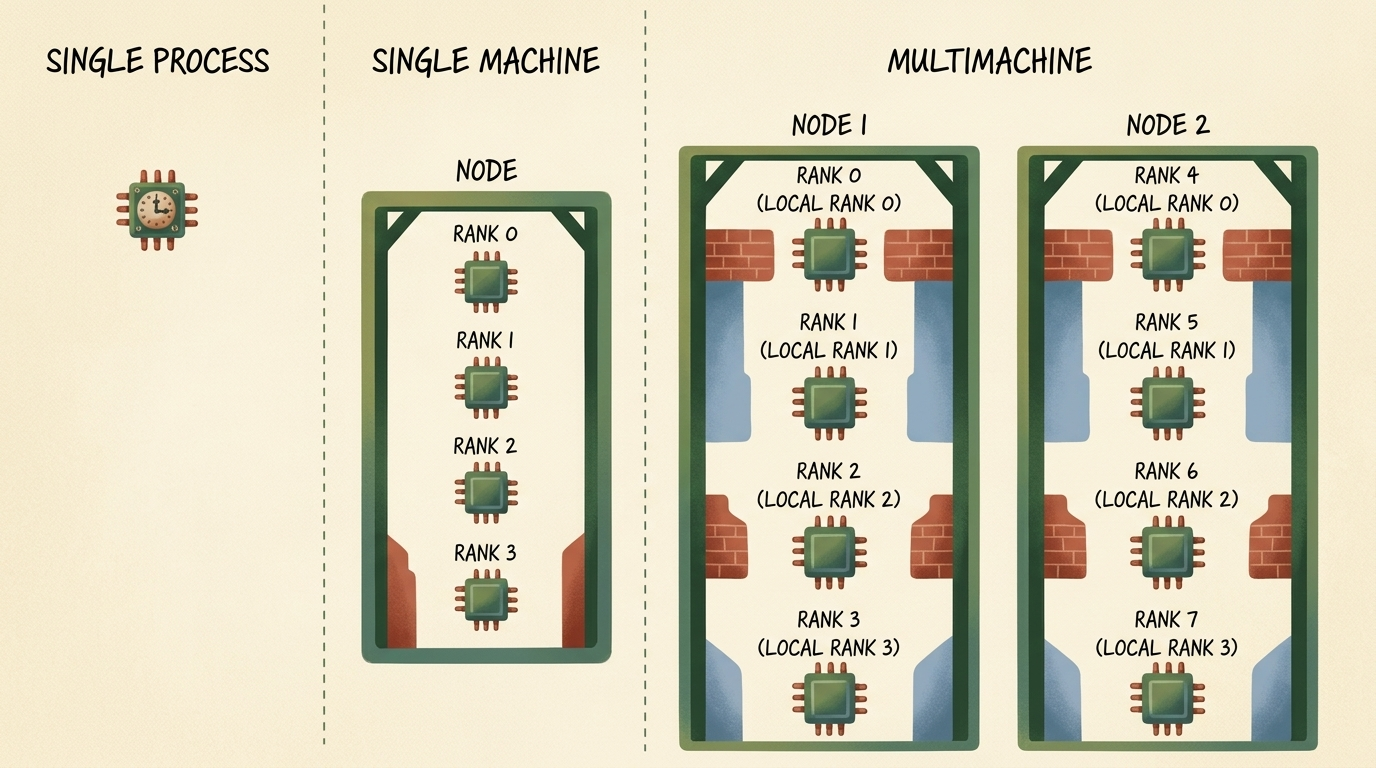
2.1 Core Terminology: World Size, Rank, and Local Rank
A distributed PyTorch program operates as a cluster of concurrent processes collaborating across a communication mesh:
- Node (Machine): A physical server motherboard containing its own CPU sockets, system RAM, network interface cards (NICs), and PCIe slots holding one or more GPUs.
- World Size ($W$): The total integer count of participating worker processes across the entire distributed cluster. If a cluster contains $N$ machines with $G$ GPUs each, the total world size is:
$$ W = N \times G $$
- Rank ($r$): The unique global integer identifier assigned to each process in the distributed group, satisfying:
$$ r \in {0, 1, 2, \dots, W - 1} $$
Process $r = 0$ is traditionally designated as the Master Rank (or Coordinator Rank), responsible for coordinating rendezvous discovery, logging global metrics, and saving master checkpoint binaries.
- Local Rank ($l$): The zero-indexed position of a worker process relative only to the specific physical node it resides on:
$$ l \in {0, 1, \dots, G - 1} $$
For example, in a 2-node cluster with 4 GPUs per node ($W = 8$), the process executing on Node 2 with global rank $r = 5$ has local rank $l = 1$, which maps directly to hardware device cuda:1 on that physical motherboard.
flowchart TD
subgraph MultiNode ["Distributed Cluster Architecture (World Size W = 8)"]
direction TB
subgraph Node1 ["Node 1 (Master Host: 10.0.0.1)"]
direction TB
P0["Process Rank 0<br/>(Local Rank 0 -> cuda:0)"]
P1["Process Rank 1<br/>(Local Rank 1 -> cuda:1)"]
P2["Process Rank 2<br/>(Local Rank 2 -> cuda:2)"]
P3["Process Rank 3<br/>(Local Rank 3 -> cuda:3)"]
end
subgraph Node2 ["Node 2 (Worker Host: 10.0.0.2)"]
direction TB
P4["Process Rank 4<br/>(Local Rank 0 -> cuda:0)"]
P5["Process Rank 5<br/>(Local Rank 1 -> cuda:1)"]
P6["Process Rank 6<br/>(Local Rank 2 -> cuda:2)"]
P7["Process Rank 7<br/>(Local Rank 3 -> cuda:3)"]
end
Node1 <== "InfiniBand / RoCE Interconnect (100 - 400 Gbps)" ==> Node2
end
style MultiNode fill:#1a1a2e,stroke:#4cc9f0,stroke-width:2px,color:#fff
style Node1 fill:#16213e,stroke:#52b788,stroke-width:1px,color:#fff
style Node2 fill:#16213e,stroke:#f77f00,stroke-width:1px,color:#fff
style P0 fill:#0f3460,stroke:#52b788,stroke-width:1px,color:#fff
style P1 fill:#0f3460,stroke:#52b788,stroke-width:1px,color:#fff
style P2 fill:#0f3460,stroke:#52b788,stroke-width:1px,color:#fff
style P3 fill:#0f3460,stroke:#52b788,stroke-width:1px,color:#fff
style P4 fill:#0f3460,stroke:#f77f00,stroke-width:1px,color:#fff
style P5 fill:#0f3460,stroke:#f77f00,stroke-width:1px,color:#fff
style P6 fill:#0f3460,stroke:#f77f00,stroke-width:1px,color:#fff
style P7 fill:#0f3460,stroke:#f77f00,stroke-width:1px,color:#fff
2.2 Hardware Interconnects: NVLink, PCIe, and InfiniBand
The choice of physical interconnect strictly governs which distributed parallelism strategy is viable:
| Interconnect Technology | Physical Scope | Unidirectional Bandwidth | Typical Round-Trip Latency | Ideal Parallelism Strategy |
|---|---|---|---|---|
| PCIe Gen4 / Gen5 | Intra-Node (Motherboard Bus) | $32\text{–}64\text{ GB/s}$ | $\sim 1\text{–}2\ \mu\text{s}$ | Data Parallelism (DDP) |
| NVIDIA NVLink / NVSwitch | Intra-Node (Dedicated Mesh) | $300\text{–}900\text{ GB/s}$ | $< 1\ \mu\text{s}$ | Tensor Parallelism (TP), FSDP |
| InfiniBand (HDR/NDR) / RoCE | Inter-Node (Network Fabric) | $25\text{–}50\text{ GB/s}$ ($200\text{–}400\text{ Gbps}$) | $\sim 2\text{–}5\ \mu\text{s}$ | Data Parallelism (DDP), Pipeline Parallelism (PP) |
| Standard Ethernet (1GbE/10GbE) | Inter-Node (Standard LAN) | $0.125\text{–}1.25\text{ GB/s}$ | $\sim 50\text{–}100\ \mu\text{s}$ | Asynchronous Training, Small DDP |
3. Process Lifecycle & Bootstrapping: From mp.spawn to torchrun
Transforming a single-device script into a distributed cluster execution follows a strict three-phase lifecycle: process creation, communication rendezvous, and distributed-aware training execution.
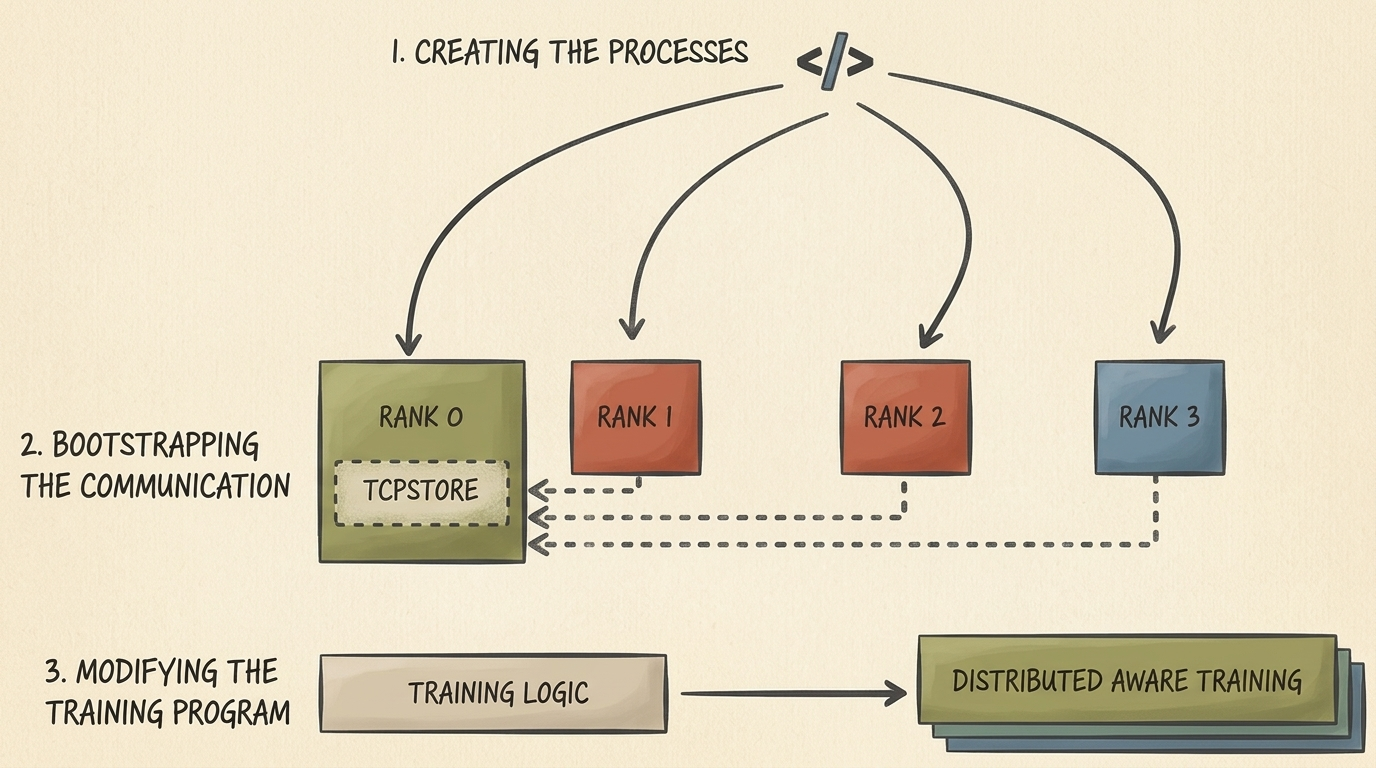
3.1 Step 1 & 2: Process Spawning and TCPStore Rendezvous
In Python, each participating rank must run in its own independent operating system process to bypass the Python Global Interpreter Lock (GIL). In early PyTorch workflows, developers explicitly spawned processes using torch.multiprocessing:
The code below initializes a distributed cluster using torch.multiprocessing.spawn and sets up a dist.TCPStore instance on the master node so that worker ranks can register their network addresses:
import os
import torch
import torch.distributed as dist
import torch.multiprocessing as mp
def init_process_with_store(rank: int, world_size: int, backend: str = "gloo"):
"""
Manually bootstraps a distributed process group using TCPStore rendezvous.
Processes connect to MASTER_ADDR:MASTER_PORT where Rank 0 hosts the store.
"""
master_addr = os.environ.get("MASTER_ADDR", "localhost")
master_port = int(os.environ.get("MASTER_PORT", "12355"))
# Instantiate the key-value store for process group rendezvous
store = dist.TCPStore(
host_name=master_addr,
port=master_port,
world_size=world_size,
is_master=(rank == 0)
)
# Initialize the default distributed process group
dist.init_process_group(
backend=backend,
store=store,
rank=rank,
world_size=world_size
)
print(f"[Rank {rank}/{world_size}] Initialized successfully with backend: {backend}")
# Synchronize all processes to guarantee clean cluster startup
dist.barrier()
# Tear down communication channels when execution finishes
dist.destroy_process_group()
if __name__ == "__main__":
num_processes = 4
os.environ["MASTER_ADDR"] = "localhost"
os.environ["MASTER_PORT"] = "12355"
# mp.spawn automatically passes the process index (0 to num_processes - 1) as argument 1
mp.spawn(
init_process_with_store,
args=(num_processes, "gloo"),
nprocs=num_processes,
join=True
)
3.2 Step 3: Modern Distributed Orchestration via torchrun
While mp.spawn is instructive for understanding low-level process creation, modern production distributed PyTorch relies on the torchrun command-line utility.
torchrun eliminates manual store initialization, automatically detects hardware accelerators, sets cluster environment variables (RANK, LOCAL_RANK, WORLD_SIZE, MASTER_ADDR, MASTER_PORT), and provides automatic fault tolerance with elastic worker restarting:
# Launch a 4-process distributed training job on a single machine
torchrun --standalone --nproc-per-node=4 train_distributed.py
# Launch on a multi-node cluster (executing on Node 1 with 2 total nodes)
torchrun --nproc-per-node=8 \
--nnodes=2 \
--node-rank=0 \
--master-addr="10.0.0.1" \
--master-port=29500 \
train_distributed.py
Inside train_distributed.py, the initialization code shrinks to a clean, minimal contract:
import os
import torch
import torch.distributed as dist
def init_distributed():
"""
Standard production distributed initialization reading environment variables
injected automatically by the torchrun launcher.
"""
# Initialize process group; backend defaults to 'nccl' on CUDA, 'gloo' on CPU
backend = "nccl" if torch.cuda.is_available() else "gloo"
dist.init_process_group(backend=backend)
local_rank = int(os.environ["LOCAL_RANK"])
global_rank = int(os.environ["RANK"])
world_size = int(os.environ["WORLD_SIZE"])
if torch.cuda.is_available():
# Bind the current process to its dedicated physical GPU device
torch.cuda.set_device(local_rank)
device = torch.device(f"cuda:{local_rank}")
else:
device = torch.device("cpu")
print(f"[Rank {global_rank}/{world_size}] Bound to local accelerator device: {device}")
return device, global_rank, local_rank, world_size
3.3 Communication Backends: NCCL vs. Gloo
The backend argument in dist.init_process_group designates the underlying low-level transport engine:
nccl(NVIDIA Collective Communications Library): The gold standard for GPU-to-GPU communication. Implements hardware-accelerated Ring-AllReduce and Tree-AllReduce algorithms over NVLink and InfiniBand with GPUDirect RDMA (Remote Direct Memory Access, bypassing host CPU RAM entirely).gloo: A portable collective communications library developed by Meta. Required for CPU-only clusters or testing environments (such as Windows environments lacking native NCCL support). While Gloo can technically handle GPU tensors, it does so by staging tensors through host CPU RAM, incurring severe PCIe latency penalties.
4. Collective Communication Primitives
Distributed deep learning algorithms do not exchange ad-hoc point-to-point messages; they rely on structured mathematical operations termed Collectives. Every rank in the active ProcessGroup participates concurrently in collective operations.
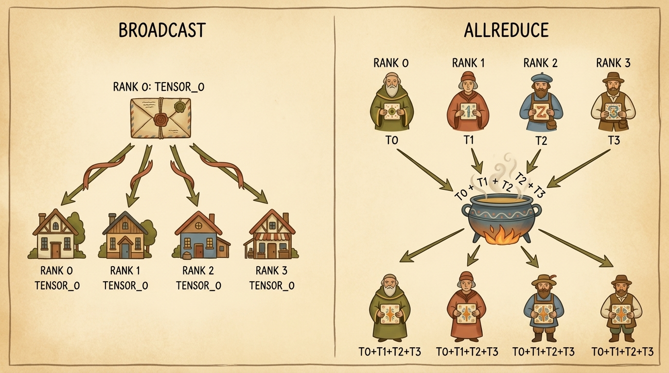
4.1 Broadcast vs. AllReduce: Mechanics and Algorithms
The two foundational collectives illustrated above serve distinct functional purposes in training:
1. Broadcast (One-to-All)
A single designated root rank (src=0) transmits its local tensor $\mathbf{T}_0$ to every process in the group. Upon completion, every rank holds an exact replica of $\mathbf{T}_0$:
$$ \mathbf{T}_r \leftarrow \mathbf{T}_{\text{src}}, \quad \forall r \in {0, \dots, W-1} $$
Primary Application: Synchronizing initial randomized model weights $\theta_0$ across all workers at epoch 0 so every GPU starts from the exact same parameter coordinates.
2. AllReduce (All-to-All Reduction)
Every rank starts with its own local tensor $\mathbf{T}_r$. A specified associative reduction operator $\oplus$ (such as summation $\sum$ or average) combines the tensors element-wise across all ranks. The resulting reduced tensor $\mathbf{T}^*$ is copied back to all ranks:
$$ \mathbf{T}^* = \bigoplus_{r=0}^{W-1} \mathbf{T}_r = \sum_{r=0}^{W-1} \mathbf{T}_r $$
$$ \mathbf{T}_r \leftarrow \mathbf{T}^*, \quad \forall r \in {0, \dots, W-1} $$
Primary Application: Synchronizing autograd gradient tensors ($\nabla_\theta \mathcal{L}$) across all data-parallel replicas after every backward pass.
4.2 The Ring-AllReduce Algorithm & Bandwidth Optimality
Naively routing all tensors to Rank 0 for summation and broadcasting the result creates a fatal network bottleneck on Rank 0. Modern distributed systems execute Ring-AllReduce:
- Logically arrange the $W$ ranks into a unidirectional ring: $\text{Rank } 0 \to \text{Rank } 1 \to \dots \to \text{Rank } (W-1) \to \text{Rank } 0$.
- Split each tensor of size $M$ elements into $W$ equal chunks: $\mathbf{T} = [C_0, C_1, \dots, C_{W-1}]$, each of size $\frac{M}{W}$.
- Scatter-Reduce Phase ($W-1$ communication steps): In step $k$, rank $r$ sends chunk $(r - k) \pmod W$ to rank $(r + 1)$ and simultaneously receives chunk $(r - k - 1) \pmod W$ from rank $(r - 1)$, accumulating received values into its local buffer. After $W-1$ steps, each rank holds the fully reduced sum of one chunk.
- AllGather Phase ($W-1$ communication steps): Each rank transmits its fully reduced chunk around the ring so all ranks receive all reduced chunks.
The total volume of data transmitted by each rank across both phases is:
$$ \text{Data Transferred per Rank} = 2 \times \frac{W - 1}{W} \times M \approx 2M \quad (\text{as } W \to \infty) $$
Key Insight: The network communication volume per GPU in Ring-AllReduce is completely independent of the cluster size $W$! Adding more GPUs to the cluster does not increase the per-GPU communication payload, providing optimal weak scaling.
4.3 Collective Operations in PyTorch Code
The snippet below demonstrates broadcast and all-reduce operations executing across ranks:
import torch
import torch.distributed as dist
def run_collectives_demo(rank: int, world_size: int, device: torch.device):
"""
Demonstrates broadcast and all_reduce collective communications in PyTorch.
"""
# 1. Demonstration of Broadcast
if rank == 0:
# Rank 0 creates the definitive initialization payload
payload = torch.tensor([42.0, 99.0, 108.0], dtype=torch.float32, device=device)
else:
# Other ranks allocate uninitialized receptor memory of identical shape and dtype
payload = torch.zeros(3, dtype=torch.float32, device=device)
print(f"Before Broadcast [Rank {rank}]: {payload}")
# Broadcast from src=0 to all ranks in the group
dist.broadcast(payload, src=0)
print(f"After Broadcast [Rank {rank}]: {payload}")
dist.barrier()
# 2. Demonstration of AllReduce
# Each rank generates a unique local tensor proportional to its rank ID
local_tensor = torch.tensor([float(rank) + 1.0, float(rank) * 10.0], device=device)
print(f"Before AllReduce [Rank {rank}]: {local_tensor}")
# Sum elements across all ranks and distribute the sum to every rank
dist.all_reduce(local_tensor, op=dist.ReduceOp.SUM)
print(f"After AllReduce SUM [Rank {rank}]: {local_tensor}")
# Calculate global average: divide by world size
local_tensor /= world_size
print(f"Global Average [Rank {rank}]: {local_tensor}")
5. Data Parallelism & DistributedDataParallel (DDP)
Data Parallelism is the most widespread and efficient distributed scaling strategy in deep learning. In this paradigm, the entire model is replicated on every GPU, while the global training dataset is partitioned into disjoint mini-batches across workers.
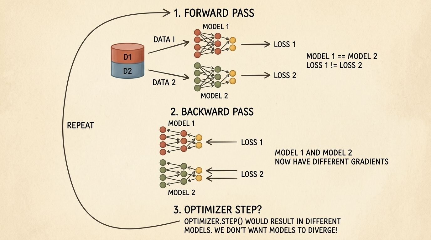
5.1 The Gradient Divergence Problem
Consider two worker devices ($W = 2$). At step $t$, both start with identical parameter weights $\theta_t$:
- Worker 1 ingests mini-batch $\mathcal{B}_1 \sim \mathcal{D}$ and computes loss $\mathcal{L}_1(\theta_t; \mathcal{B}_1)$ and gradients $\mathbf{g}_1 = \nabla_\theta \mathcal{L}_1$.
- Worker 2 ingests mini-batch $\mathcal{B}_2 \sim \mathcal{D}$ and computes loss $\mathcal{L}_2(\theta_t; \mathcal{B}_2)$ and gradients $\mathbf{g}_2 = \nabla_\theta \mathcal{L}_2$.
Because $\mathcal{B}_1 \neq \mathcal{B}_2$, the individual gradients differ:
$$ \mathbf{g}_1 \neq \mathbf{g}_2 $$
If each worker immediately updates its local weights using an optimizer (e.g., SGD: $\theta_{t+1}^{(i)} = \theta_t - \eta \mathbf{g}_i$), the two models immediately diverge into entirely separate parameter spaces:
$$ \theta_{t+1}^{(1)} \neq \theta_{t+1}^{(2)} $$
To maintain mathematical equivalence with a large single-GPU batch of size $B_{\text{global}} = W \times B_{\text{local}}$, workers must synchronize their gradients via an AllReduce average before updating weights:
$$ \bar{\mathbf{g}} = \frac{1}{W} \sum_{i=1}^W \mathbf{g}_i $$
$$ \theta_{t+1} = \theta_t - \eta \bar{\mathbf{g}} $$
5.2 Internal Architecture of DistributedDataParallel (DDP)
PyTorch provides two data-parallel wrappers: torch.nn.DataParallel (DP) and torch.nn.parallel.DistributedDataParallel (DDP).
Warning
Never use
torch.nn.DataParallel:DataParallelis a legacy single-process, multi-threaded wrapper subject to Python’s GIL. It gathers all outputs on GPU 0 to calculate loss, creating severe GPU 0 memory imbalances and massive PCIe transmission bottlenecks. Always use multi-processDistributedDataParallel(DDP).
DDP achieves high performance through two architectural mechanisms:
- Autograd Backward Hooks & Overlapping: Rather than waiting for the entire backward pass to finish before starting network transfers, DDP registers autograd backward hooks on individual parameter tensors. The moment a layer finishes computing its gradients, DDP immediately dispatches an asynchronous non-blocking AllReduce call over the network while earlier layers are still computing their backward pass on the GPU.
- Gradient Bucketing: Communicating millions of tiny gradient tensors individually incurs overwhelming network latency overhead. DDP groups parameters into contiguous memory buffers called buckets (typically 25 MB each). An AllReduce collective is triggered only when an entire bucket fills with computed gradients.
flowchart TD
subgraph DDPExecution ["DDP Overlapped Execution Flow (Per Iteration)"]
direction TB
F1["Forward Pass (Layer 1 -> Layer L)<br/>Computed completely locally on each GPU"]
B_Last["Backward Pass on Layer L<br/>Computes Gradient g_L locally"]
Bucket["Fill Gradient Bucket (e.g. 25 MB)<br/>Parameters aggregated in memory buffer"]
Comm["Async Background AllReduce<br/>Overlapped with compute via NCCL Streams"]
B_Earlier["Backward Pass on Layer L-1, L-2...<br/>Computes earlier gradients concurrently on GPU"]
Sync["All Buckets Reduced & Synchronized"]
Opt["Optimizer Step (Identical update on all ranks)"]
F1 --> B_Last --> Bucket --> Comm
B_Last --> B_Earlier
Comm & B_Earlier --> Sync --> Opt
end
style DDPExecution fill:#1a1a2e,stroke:#4cc9f0,stroke-width:2px,color:#fff
style F1 fill:#16213e,stroke:#4cc9f0,stroke-width:1px,color:#fff
style B_Last fill:#1a3a2a,stroke:#52b788,stroke-width:1px,color:#fff
style Bucket fill:#1a3a2a,stroke:#52b788,stroke-width:1px,color:#fff
style Comm fill:#3a2a1a,stroke:#f77f00,stroke-width:2px,color:#fff
style B_Earlier fill:#1a3a2a,stroke:#52b788,stroke-width:1px,color:#fff
style Sync fill:#0f3460,stroke:#4cc9f0,stroke-width:1px,color:#fff
style Opt fill:#16213e,stroke:#4cc9f0,stroke-width:1px,color:#fff
5.3 Deterministic Data Sharding with DistributedSampler
To ensure each rank ingests non-overlapping training samples, we wrap our Dataset inside a torch.utils.data.distributed.DistributedSampler.
The sampler splits the dataset indices into $W$ subsets. Calling sampler.set_epoch(epoch) before each training epoch guarantees deterministic yet diverse shuffling across epochs:
import torch
import torch.nn as nn
from torch.utils.data import Dataset, DataLoader
from torch.utils.data.distributed import DistributedSampler
from torch.nn.parallel import DistributedDataParallel as DDP
def setup_ddp_training(rank: int, world_size: int, device: torch.device, dataset: Dataset):
"""
Constructs a complete production DDP pipeline with DistributedSampler.
"""
# 1. Instantiate the neural network and move it to the process-assigned GPU
model = nn.Sequential(
nn.Linear(128, 256),
nn.ReLU(),
nn.Linear(256, 10)
).to(device)
# 2. Wrap model in DDP; broadcast_buffers=False prevents unnecessary buffer syncs
ddp_model = DDP(
model,
device_ids=[device.index] if device.type == "cuda" else None,
output_device=device.index if device.type == "cuda" else None,
find_unused_parameters=False
)
# 3. Configure DistributedSampler for disjoint batch feeding
sampler = DistributedSampler(
dataset,
num_replicas=world_size,
rank=rank,
shuffle=True,
drop_last=True
)
# Critical: batch_size specifies samples PER GPU, not total cluster batch!
loader = DataLoader(
dataset,
batch_size=32,
sampler=sampler,
num_workers=4,
pin_memory=True
)
optimizer = torch.optim.AdamW(ddp_model.parameters(), lr=1e-3)
criterion = nn.CrossEntropyLoss()
# 4. Standard training loop with epoch seeding
for epoch in range(5):
# Mandatory: seeds the pseudo-random generator across ranks for this epoch
sampler.set_epoch(epoch)
ddp_model.train()
for batch_idx, (inputs, targets) in enumerate(loader):
inputs = inputs.to(device, non_blocking=True)
targets = targets.to(device, non_blocking=True)
optimizer.zero_grad()
outputs = ddp_model(inputs)
loss = criterion(outputs, targets)
# Autograd backward: DDP hooks automatically trigger bucketed AllReduce
loss.backward()
# All gradients are now identical across all ranks
optimizer.step()
6. Model Parallelism: Splitting Massive Architectures
While Data Parallelism replicates the model on every GPU, modern deep learning architectures often exceed the memory capacity of a single GPU.
6.1 The GPU Memory Consumption Breakdown
During training, GPU High Bandwidth Memory (HBM) is consumed by four distinct memory pools:
- Model Parameters ($\Phi$): Storing weights in 32-bit floating point requires $4\Phi$ bytes (or $2\Phi$ bytes in FP16/BF16).
- Autograd Gradients: Requires matching storage to model parameters ($4\Phi$ bytes in FP32).
- Optimizer States: The standard AdamW optimizer maintains two 32-bit tracking moments per parameter (running first moment $m_t$ and second moment $v_t$) plus FP32 master weights, totaling $12\Phi$ to $16\Phi$ bytes!
- Intermediate Activations & KV Caches: All forward intermediate activations required for backward gradient computation.
For a 7-billion parameter ($7\text{B}$) model:
$$ \text{Static Memory} \approx 4\Phi (\text{params}) + 4\Phi (\text{grads}) + 12\Phi (\text{AdamW}) = 20\Phi \approx 140\text{ GB} $$
A $140\text{ GB}$ footprint cannot fit onto an 80 GB NVIDIA H100 or A100 GPU. We must divide the model itself across multiple devices—a paradigm known as Model Parallelism.
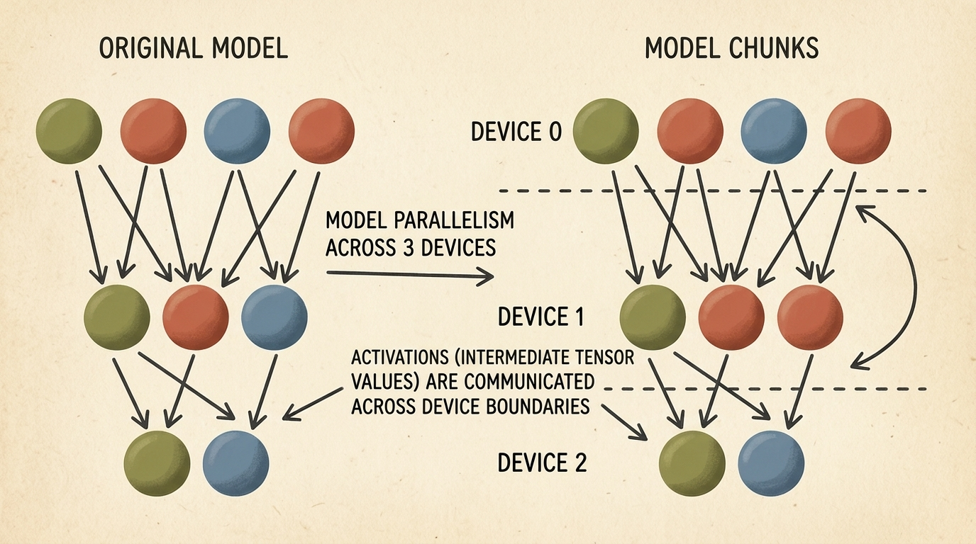
7. Pipeline Parallelism (PP) & Microbatching
When dividing a model across layers, consecutive layers are placed on separate accelerators: Device 0 computes layers 1 to $K$, Device 1 computes layers $K+1$ to $2K$, and so on. This approach is called Pipeline Parallelism (PP).
However, naive inter-layer partitioning suffers from severe device under-utilization: while Device 1 is computing, Device 0 and Device 2 sit completely idle, waiting for activations. The fraction of wasted time is known as the Pipeline Bubble.
7.1 The Pipeline Bubble & Microbatching Mechanics
To reduce bubble overhead, Pipeline Parallelism splits each training mini-batch into $M$ smaller microbatches:
- As soon as Device 0 finishes the forward pass on Microbatch 0, it sends intermediate activations to Device 1 and immediately begins computing Microbatch 1.
- In modern 1F1B (One Forward, One Backward) scheduling, devices alternate between executing one forward microbatch and one backward microbatch once the pipeline warms up, keeping activation memory bounded.
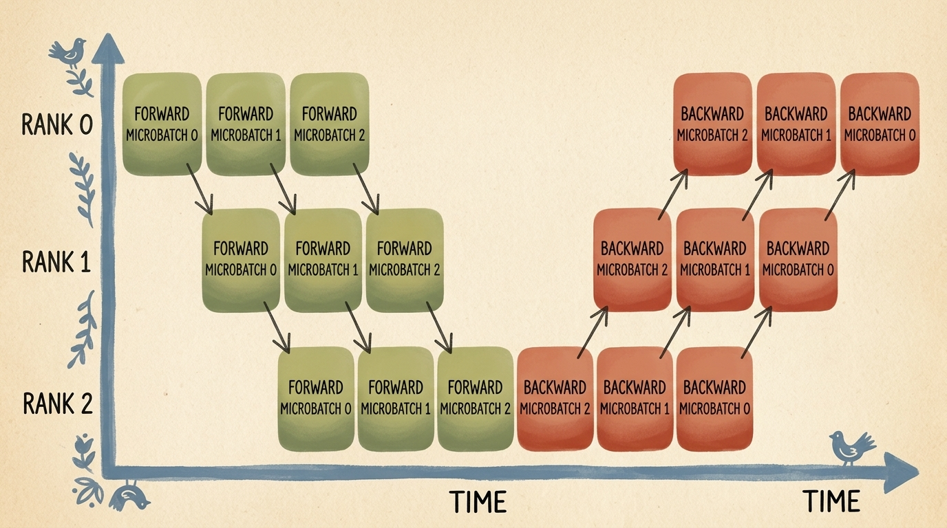
7.2 Mathematical Formulation of the Pipeline Bubble
For a pipeline consisting of $K$ pipeline stages (devices) and $M$ microbatches, the theoretical bubble fraction $F_{\text{bubble}}$ in a GPipe schedule is:
$$ F_{\text{bubble}} = \frac{K - 1}{M + K - 1} $$
As the number of microbatches $M$ grows significantly larger than the stage count $K$ ($M \gg K$), the bubble fraction approaches zero:
$$ \lim_{M \to \infty} F_{\text{bubble}} = 0 $$
However, increasing $M$ increases the number of un-freed activation tensors stored in memory simultaneously, creating a direct trade-off between memory footprint and hardware efficiency.
8. Tensor Parallelism (TP) vs. Pipeline Parallelism
While Pipeline Parallelism partitions models inter-layer (between layers), Tensor Parallelism (TP) partitions individual weight matrices intra-layer (within each layer).
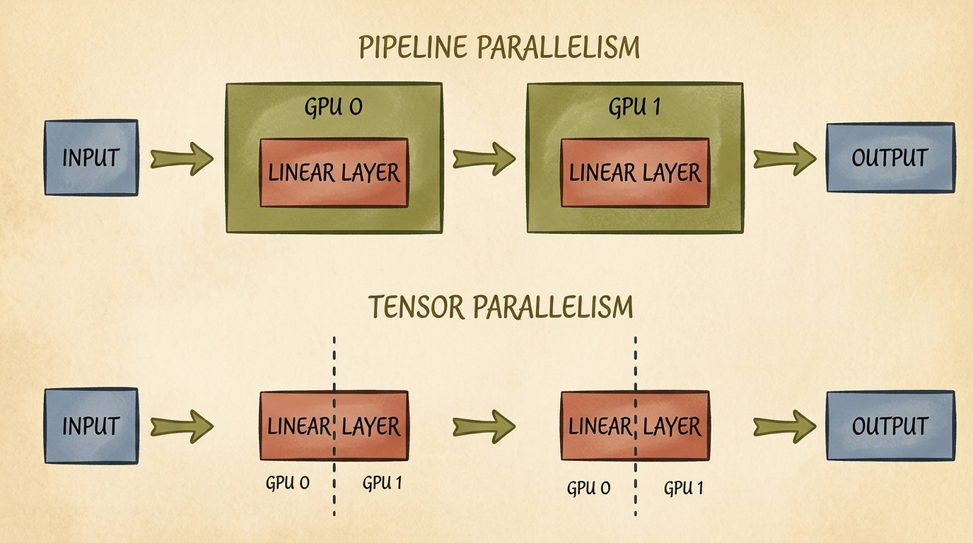
8.1 The Megatron-LM Tensor Parallel Formulation
In deep networks, multi-layer perceptrons (MLPs) and self-attention projections are composed of consecutive matrix multiplications:
$$ \mathbf{Z} = \text{GELU}(\mathbf{X} \mathbf{W}_1) \mathbf{W}_2 $$
Megatron-LM parallelizes this operation across two devices by pairing a Column-Parallel Linear layer with a Row-Parallel Linear layer:
Step 1: Column-Parallel Projection
We split weight matrix $\mathbf{W}_1 \in \mathbb{R}^{d_{\text{in}} \times d_{\text{mid}}}$ along its column dimension into two equal halves: $\mathbf{W}_1 = [\mathbf{W}_{1,1} \mid \mathbf{W}_{1,2}]$. Both GPUs receive the full input $\mathbf{X}$ and compute their local projection independently without communication:
$$ \mathbf{Y}_1 = \mathbf{X} \mathbf{W}_{1,1}, \quad \mathbf{Y}_2 = \mathbf{X} \mathbf{W}_{1,2} $$
$$ \mathbf{A}_1 = \text{GELU}(\mathbf{Y}_1), \quad \mathbf{A}_2 = \text{GELU}(\mathbf{Y}_2) $$
Step 2: Row-Parallel Projection
We split the second weight matrix $\mathbf{W}_2 \in \mathbb{R}^{d_{\text{mid}} \times d_{\text{out}}}$ along its row dimension:
$$ \mathbf{W}_2 = \begin{bmatrix} \mathbf{W}_{2,1} \\ \mathbf{W}_{2,2} \end{bmatrix} $$
Each GPU computes its local matrix product:
$$ \mathbf{Z}_1 = \mathbf{A}_1 \mathbf{W}_{2,1}, \quad \mathbf{Z}_2 = \mathbf{A}_2 \mathbf{W}_{2,2} $$
The mathematical sum of the two products yields the exact global result:
$$ \mathbf{Z} = \mathbf{Z}_1 + \mathbf{Z}_2 = \mathbf{A}_1 \mathbf{W}_{2,1} + \mathbf{A}_2 \mathbf{W}_{2,2} $$
To produce $\mathbf{Z}$, the two GPUs execute a single AllReduce (SUM) collective.
Key Architectural Insight: Across a two-layer MLP block, Tensor Parallelism requires only one AllReduce communication in the forward pass and one AllReduce communication in the backward pass!
8.2 Architectural Trade-Offs: TP vs. PP
| Characteristic | Tensor Parallelism (TP) | Pipeline Parallelism (PP) |
|---|---|---|
| Partitioning Axis | Intra-layer (splits matrices) | Inter-layer (splits layers) |
| Communication Frequency | Every single layer (high frequency) | Once per pipeline stage (low frequency) |
| Communication Volume | High volume of activation slices | Small boundary activation tensors |
| Hardware Requirement | Strictly intra-node NVLink ($>300\text{ GB/s}$) | Inter-node InfiniBand / PCIe ($25\text{–}50\text{ GB/s}$) |
| Bubble Overhead | Zero bubble overhead ($F_{\text{bubble}} = 0$) | Bubbles exist ($F_{\text{bubble}} = \frac{K-1}{M+K-1}$) |
| Scalability Limit | Typically capped at 8 GPUs (single node) | Scales across dozens of physical nodes |
9. N-Dimensional Parallelism & PyTorch DeviceMesh
Real-world foundation models cannot rely solely on one parallelism strategy; they compose multiple techniques simultaneously in a multi-dimensional grid.
For instance, an 8-GPU node cluster can be organized into a 2D Device Mesh combining Data Parallelism across replicas and Tensor Parallelism across model partitions.
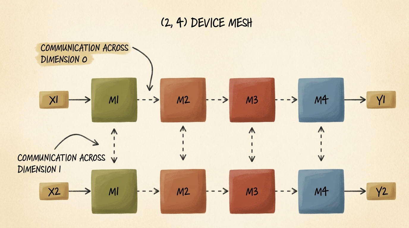
9.1 PyTorch 2.x init_device_mesh Implementation
PyTorch 2.x introduced the DeviceMesh abstraction to eliminate tedious manual calculation of process ranks and communicators.
The code below configures a 2D (2, 4) device mesh spanning 8 GPUs:
import os
import torch
import torch.distributed as dist
from torch.distributed.device_mesh import init_device_mesh
def setup_2d_device_mesh():
"""
Initializes a 2D DeviceMesh with 2 data-parallel replicas and 4 tensor-parallel ranks.
Requires an 8-GPU cluster launched via torchrun --nproc-per-node=8.
"""
dist.init_process_group(backend="nccl")
local_rank = int(os.environ["LOCAL_RANK"])
torch.cuda.set_device(local_rank)
# Construct a 2D mesh grid of shape (2, 4)
# Dimension 0 ('dp'): 2 data-parallel groups of size 4
# Dimension 1 ('tp'): 4 tensor-parallel groups of size 2
mesh_2d = init_device_mesh(
device_type="cuda",
mesh_shape=(2, 4),
mesh_dim_names=("dp", "tp")
)
dp_group = mesh_2d["dp"]
tp_group = mesh_2d["tp"]
print(f"[Rank {dist.get_rank()}] Full Mesh: {mesh_2d}")
print(f"[Rank {dist.get_rank()}] DP Sub-Mesh: {dp_group}, TP Sub-Mesh: {tp_group}")
return mesh_2d
10. Fully Sharded Data Parallelism (FSDP / ZeRO)
While traditional DDP replicates all weights, gradients, and optimizer states across every GPU, Fully Sharded Data Parallelism (FSDP)—based on the DeepSpeed ZeRO-3 (Zero Redundancy Optimizer) paper—shards all three state components across data-parallel ranks.
10.1 The ZeRO Memory Sharding Hierarchy
The ZeRO protocol defines three progressive levels of memory de-duplication:
- ZeRO-1 ($\text{P}_{\text{os}}$): Optimizer states are partitioned across $W$ ranks ($4\times$ memory reduction).
- ZeRO-2 ($\text{P}_{\text{os+g}}$): Optimizer states and autograd gradients are both partitioned ($8\times$ memory reduction).
- ZeRO-3 / FSDP ($\text{P}_{\text{os+g+p}}$): Optimizer states, gradients, and model parameters are all partitioned across $W$ ranks. Each GPU stores only $\frac{1}{W}$ of the entire model footprint during resting state!
flowchart TD
subgraph FSDPLifecycle ["FSDP Layer-by-Layer Execution Lifecycle"]
direction TB
subgraph Forward ["Forward Pass (Per Layer i)"]
direction TB
AG_Fwd["1. AllGather Layer i Full Weights<br/>Collect shards from all W ranks into local VRAM"]
Compute_Fwd["2. Compute Forward Activation<br/>Output y_i = Layer_i(x_i)"]
Free_Fwd["3. Discard Full Layer i Weights<br/>Free temporary buffer, retain only local 1/W shard"]
AG_Fwd --> Compute_Fwd --> Free_Fwd
end
subgraph Backward ["Backward Pass (Per Layer i in reverse)"]
direction TB
AG_Bwd["1. AllGather Layer i Full Weights<br/>Reconstruct weights for autograd derivative"]
Compute_Bwd["2. Compute Gradients dl/dx and dl/dw"]
Free_Bwd["3. Discard Full Weights<br/>Instantly release full weight memory"]
RS_Bwd["4. ReduceScatter Gradients<br/>Sum gradients and scatter 1/W shards to owners"]
AG_Bwd --> Compute_Bwd --> Free_Bwd --> RS_Bwd
end
Forward --> Backward
end
style FSDPLifecycle fill:#1a1a2e,stroke:#4cc9f0,stroke-width:2px,color:#fff
style Forward fill:#16213e,stroke:#52b788,stroke-width:1px,color:#fff
style Backward fill:#16213e,stroke:#f77f00,stroke-width:1px,color:#fff
style AG_Fwd fill:#0f3460,stroke:#52b788,stroke-width:1px,color:#fff
style Compute_Fwd fill:#0f3460,stroke:#52b788,stroke-width:1px,color:#fff
style Free_Fwd fill:#2b1b22,stroke:#e63946,stroke-width:1px,color:#fff
style AG_Bwd fill:#0f3460,stroke:#f77f00,stroke-width:1px,color:#fff
style Compute_Bwd fill:#0f3460,stroke:#f77f00,stroke-width:1px,color:#fff
style Free_Bwd fill:#2b1b22,stroke:#e63946,stroke-width:1px,color:#fff
style RS_Bwd fill:#0f3460,stroke:#f77f00,stroke-width:1px,color:#fff
10.2 Modern PyTorch 2.x fully_shard API
In PyTorch 2.x, FSDP was completely redesigned into the clean, composable fully_shard API:
import torch
import torch.nn as nn
from torch.distributed.device_mesh import init_device_mesh
from torch.distributed.fsdp import fully_shard
class DeepTransformerBlock(nn.Module):
def __init__(self, dim: int = 1024):
super().__init__()
self.fc1 = nn.Linear(dim, dim * 4)
self.relu = nn.ReLU()
self.fc2 = nn.Linear(dim * 4, dim)
def forward(self, x: torch.Tensor) -> torch.Tensor:
return x + self.fc2(self.relu(self.fc1(x)))
def apply_fsdp_sharding(model: nn.Module, mesh):
"""
Shards sub-modules individually and then shards the top-level container.
"""
# 1. Shard individual building blocks for fine-grained forward AllGather/freeing
for module in model.modules():
if isinstance(module, DeepTransformerBlock):
fully_shard(module, mesh=mesh)
# 2. Shard root model container
fully_shard(model, mesh=mesh)
return model
11. Advanced LLM Parallelisms: Context & Expert Parallelism
When training generative transformers (Section 2.1) on extreme sequence lengths or sparse architectures, two specialized distributed strategies become indispensable:
11.1 Context Parallelism (CP) and Ring Attention
Standard multi-head attention scales quadratically with sequence length $L$:
$$ \text{Memory}_{\text{attn}} = \mathcal{O}(L^2) $$
When processing 128k or 1M token documents, a single accelerator’s memory is exhausted simply storing the attention score matrix $\mathbf{Q} \mathbf{K}^T$.
Context Parallelism partitions the sequence dimension $L$ across $C$ ranks so that each GPU holds only $\frac{L}{C}$ tokens. Using Ring Attention, each GPU computes attention queries $\mathbf{Q}$ locally while rotating key $\mathbf{K}$ and value $\mathbf{V}$ blocks around an intra-node ring, maintaining causal masking invariants while dividing peak activation memory by $C$.
11.2 Expert Parallelism (EP) for Mixture-of-Experts (MoE)
In modern sparse Mixture-of-Experts architectures (such as Mixtral or DeepSeek-V3), feed-forward layers are replaced with an ensemble of $E$ specialized expert networks.
Expert Parallelism assigns different expert subnetworks to different physical GPUs. During the forward pass, a learned router assigns tokens to specific experts; tokens are dispatched across GPUs using high-speed All-to-All collective communications and recombined post-computation.
12. Production Distributed Systems: TorchTitan & Summary
Orchestrating 3D/4D hybrid parallelism (combining DDP, FSDP, TP, PP, and CP) in production requires clean engineering frameworks. To showcase native, un-bloated PyTorch 2.x distributed scaling, the Meta PyTorch team released TorchTitan (github.com/pytorch/torchtitan).
TorchTitan provides clean reference implementations of LLaMA 3 and modern transformer architectures scaled across thousands of GPUs using only pure upstream PyTorch primitives without third-party wrapper bloat.
12.1 Distributed Parallelism Decision Matrix
When architecting a distributed system, select strategies based on model parameter count, cluster scale, and interconnect speed:
| Model Scale | Single GPU Feasible? | Recommended Parallelism Strategy | Critical Interconnect Requirement |
|---|---|---|---|
| < 1B Parameters (e.g. LUNA 3D CNNs) | Yes | DistributedDataParallel (DDP) | Standard PCIe / 10GbE Network |
| 1B – 15B Parameters (e.g. LLaMA-3 8B) | No | FSDP (ZeRO-3) | PCIe Gen4/5 or Intra-Node NVLink |
| 15B – 70B Parameters | No | 2D Hybrid: FSDP + Tensor Parallelism (TP) | Intra-Node NVLink + Inter-Node InfiniBand |
| > 70B Parameters | No | 3D/4D Hybrid: FSDP + TP + PP (+ CP) | Full NVLink NVSwitch + Multi-Rail InfiniBand |
flowchart TD
Start["Does the entire model, gradients, and optimizer fit on a single GPU?"]
DDP["Apply DistributedDataParallel (DDP)<br/>Fastest setup, zero bubble overhead, near-linear scaling"]
FitWithFSDP["Does model fit when parameters & optimizer are sharded across nodes?"]
FSDP["Apply Fully Sharded Data Parallelism (FSDP)<br/>ZeRO-3 sharding with overlapped AllGather/ReduceScatter"]
CheckNVLink["Do you have intra-node NVLink (>300 GB/s)?"]
TP_FSDP["Apply 2D Hybrid Parallelism<br/>Tensor Parallelism (TP) intra-node + FSDP inter-node"]
Full3D["Apply 3D Parallelism<br/>TP (intra-node) + PP (inter-node) + FSDP"]
Start -- Yes --> DDP
Start -- No --> FitWithFSDP
FitWithFSDP -- Yes --> FSDP
FitWithFSDP -- No --> CheckNVLink
CheckNVLink -- Yes --> TP_FSDP
CheckNVLink -- No --> Full3D
style Start fill:#1a1a2e,stroke:#4cc9f0,stroke-width:2px,color:#fff
style DDP fill:#1a3a2a,stroke:#52b788,stroke-width:2px,color:#fff
style FitWithFSDP fill:#16213e,stroke:#4cc9f0,stroke-width:1px,color:#fff
style FSDP fill:#1a3a2a,stroke:#52b788,stroke-width:2px,color:#fff
style CheckNVLink fill:#16213e,stroke:#4cc9f0,stroke-width:1px,color:#fff
style TP_FSDP fill:#0f3460,stroke:#4cc9f0,stroke-width:2px,color:#fff
style Full3D fill:#3a1a1a,stroke:#e63946,stroke-width:2px,color:#fff
Deploying to Production
- 1. The Production Mandate: Bridging Research and Industrial Deployment
- 2. Serving PyTorch Models: Interactive UIs vs. Industrial Microservices
- 3. Dynamic Request Batching & Token Streaming Architecture
- 4. Inference Acceleration Techniques: Precision, Quantization, and Memory Layouts
- 5. Model Graph Capture & Export: From Python Code to Static Graphs
- 6. Deep Dive into
torch.compile& The Inductor Compiler Engine - 7. Execution Profiling with
torch.profiler - 8. Python-Free Zero-Overhead Serving: LibTorch (C++)
- 9. Mobile & Edge Deployment: ExecuTorch
- 10. Production Decision Framework: Choosing the Right Deployment Stack
- 11. Exercises & Conceptual Verification
- 12. Conclusion & Summary
1. The Production Mandate: Bridging Research and Industrial Deployment
Throughout Part 1 and the preceding chapters of Part 2, our focus centered on architectural design, mathematical modeling, and training mechanics. We built convolutional vision backbones, generative diffusion pipelines, volumetric 3D tumor classification models, semantic segmentation networks, and multi-GPU distributed clusters. In all these workflows, execution occurred within an interactive Python development environment where models ran inside dedicated training loops with full access to autograd dynamic tapes, high-bandwidth accelerator memory, and the Python runtime.
However, moving a trained neural network into production requires an entirely different engineering mindset. A production environment imposes strict constraints that do not exist during model research:
- Deterministic Latency & Strict SLAs: Client applications demand responses within strict millisecond bounds. While training can tolerate varying execution times per iteration, a clinical diagnostic API or autonomous robotics loop has a non-negotiable service-level agreement (SLA) on Time to First Token (TTFT) or maximum request latency.
- High Throughput Under Concurrent Load: Serving hundreds or thousands of concurrent incoming requests saturates naive sequential inference pipelines. Production systems must aggregate distinct requests dynamically without starving individual users.
- Hardware & Runtime Isolation: Modern production backends often cannot afford the memory footprint, startup time, or single-threaded concurrency limitations imposed by Python’s Global Interpreter Lock (GIL). Autonomous mobile agents, automotive microcontrollers, and microsecond-scale trading engines require lightweight, self-contained binaries executing via C++ runtimes or specialized hardware compilers.
- Energy, Compute, and Memory Footprint: Running multi-billion parameter foundation models or large 3D CNNs with full 32-bit floating-point precision on cloud accelerators is economically and thermally prohibitive. Models must be quantized, fused, and compiled to minimize high-bandwidth memory (HBM) bandwidth saturation.
flowchart TD
PROD["Production Deep Learning Serving Requirements"]
PROD --> S1["1. Low-Latency Serving Layer<br/>FastAPI / Gradio / Asynchronous Endpoints"]
PROD --> S2["2. Dynamic Concurrency & Batching<br/>Async queues, batch aggregation & token streaming"]
PROD --> S3["3. Graph Optimization & Compilation<br/>ONNX, torch.export & torch.compile (Inductor)"]
PROD --> S4["4. Runtime Portability & Low Footprint<br/>Python-free LibTorch (C++) & Mobile ExecuTorch"]
S1 --> GOAL["Deterministic Sub-10ms Inference & Multi-Client Scaling"]
S2 --> GOAL
S3 --> GOAL
S4 --> GOAL
style PROD fill:#1a1a2e,stroke:#4cc9f0,stroke-width:2px,color:#fff
style S1 fill:#16213e,stroke:#52b788,stroke-width:1px,color:#fff
style S2 fill:#16213e,stroke:#52b788,stroke-width:1px,color:#fff
style S3 fill:#1a3a2a,stroke:#f77f00,stroke-width:1px,color:#fff
style S4 fill:#2b1b22,stroke:#e63946,stroke-width:1px,color:#fff
style GOAL fill:#0f3460,stroke:#4cc9f0,stroke-width:2px,color:#fff
Key Insight: In deep learning production systems, high throughput and low latency are often in direct architectural tension. Maximizing throughput requires aggregating requests into large batches to achieve high arithmetic intensity on GPU tensor cores, whereas minimizing latency demands executing inference immediately upon request arrival. Production engineering is the science of resolving this tension via dynamic batching, asynchronous streaming, and kernel-level graph compilation.
2. Serving PyTorch Models: Interactive UIs vs. Industrial Microservices
When deploying a trained PyTorch model for inference, engineers select the serving interface based on the target consumer: human evaluators or automated client applications.
2.1 Rapid Human-in-the-Loop Evaluation with Gradio
During model development, clinical trials, or user acceptance testing, engineers need an interactive interface where non-technical stakeholders can upload images, adjust parameters via sliders, and immediately inspect network predictions. Gradio provides a zero-boilerplate abstraction designed specifically for machine learning models.
The code below initializes a pretrained vision transformer and wraps it in a Gradio user interface that accepts raw image inputs, applies ImageNet normalization transforms, and displays top-5 classification probabilities in real time:
import gradio as gr
import torch
import torchvision.models as models
import torchvision.transforms as transforms
from PIL import Image
# 1. Device configuration and model initialization
device = torch.device("cuda" if torch.cuda.is_available() else "cpu")
model = models.resnet50(weights=models.ResNet50_Weights.DEFAULT)
model.eval().to(device)
# 2. Production preprocessing pipeline
preprocess = transforms.Compose([
transforms.Resize(256),
transforms.CenterCrop(224),
transforms.ToTensor(),
transforms.Normalize(
mean=[0.485, 0.456, 0.406],
std=[0.229, 0.224, 0.225]
),
])
def predict_image(image: Image.Image) -> dict:
# 3. Micro-modular inference action
tensor = preprocess(image).unsqueeze(0).to(device)
with torch.inference_mode():
logits = model(tensor)
probabilities = torch.nn.functional.softmax(logits[0], dim=0)
# 4. Extract top 5 class probabilities
top5_prob, top5_catid = torch.topk(probabilities, 5)
categories = models.ResNet50_Weights.DEFAULT.meta["categories"]
return {categories[cat_id]: float(prob) for prob, cat_id in zip(top5_prob, top5_catid)}
demo = gr.Interface(
fn=predict_image,
inputs=gr.Image(type="pil"),
outputs=gr.Label(num_top_classes=5),
title="Clinical ResNet-50 Diagnostic Demo",
description="Interactive evaluation interface for ImageNet classification."
)
Gradio is ideal for interactive demos and proof-of-concept testing. However, it is not architected for high-concurrency production microservices where hundreds of external client services make programmatic API calls over HTTP or gRPC.
2.2 Industrial Microservice Architecture with FastAPI
For programmatic production deployments, we encapsulate our PyTorch model behind FastAPI. FastAPI leverages Python’s modern asyncio event loop, strict type validation via Pydantic, and asynchronous request routing through ASGI (Asynchronous Server Gateway Interface) web servers like uvicorn.
The architectural challenge in serving deep learning models inside an asynchronous web server is avoiding event loop starvation. Standard PyTorch matrix multiplications (torch.matmul) and convolutional forwards are synchronous, CPU/GPU-blocking calls. If a heavy tensor operation runs directly inside an async def route on the main event loop thread, the entire web server locks up, unable to accept new network connections or handle health checks.
flowchart TD
subgraph ClientLayer ["Client Traffic Layer"]
C1["HTTP Client 1"]
C2["HTTP Client 2"]
C3["HTTP Client N"]
end
subgraph AsyncServer ["FastAPI Async Server (Event Loop Thread)"]
direction TB
ROUTER["FastAPI Router (/predict)<br/>Pydantic Request Validation"]
ROUTER --> NONBLOCK["Offload Blocking GPU Forward<br/>asyncio.to_thread / Background Worker"]
end
subgraph ComputeLayer ["Dedicated Compute Thread / Process"]
direction TB
T1["torch.inference_mode()<br/>FP16 Tensor Forward on GPU"]
end
C1 --> ROUTER
C2 --> ROUTER
C3 --> ROUTER
NONBLOCK --> T1
T1 -.->|Resolved Future| ROUTER
style ClientLayer fill:#1a1a2e,stroke:#4cc9f0,stroke-width:1px,color:#fff
style AsyncServer fill:#16213e,stroke:#52b788,stroke-width:2px,color:#fff
style ComputeLayer fill:#2b1b22,stroke:#e63946,stroke-width:2px,color:#fff
The code below implements an asynchronous FastAPI server that validates incoming structured requests using Pydantic, offloads tensor computation to a dedicated thread pool to keep the event loop responsive, and returns JSON inference metrics:
import asyncio
from contextlib import asynccontextmanager
from fastapi import FastAPI, HTTPException
from pydantic import BaseModel, Field
import torch
import torchvision.models as models
# 1. Pydantic request and response schemas
class InferenceRequest(BaseModel):
features: list[float] = Field(..., min_length=10, max_length=10, description="10-element input vector")
class InferenceResponse(BaseModel):
prediction: list[float]
device_used: str
# 2. Lifecycle management for global model state
ml_models = {}
@asynccontextmanager
async def lifespan(app: FastAPI):
# Setup: Allocate GPU model weights during server startup
dev = torch.device("cuda" if torch.cuda.is_available() else "cpu")
net = torch.nn.Sequential(
torch.nn.Linear(10, 64),
torch.nn.ReLU(),
torch.nn.Linear(64, 2)
).to(dev)
net.eval()
ml_models["network"] = net
ml_models["device"] = dev
yield
# Teardown: Cleanly clear CUDA allocations on shutdown
ml_models.clear()
if torch.cuda.is_available():
torch.cuda.empty_cache()
app = FastAPI(lifespan=lifespan)
def compute_forward_sync(raw_data: list[float], model: torch.nn.Module, device: torch.device) -> list[float]:
# Pure synchronous forward execution isolated from event loop
with torch.inference_mode():
x = torch.tensor([raw_data], dtype=torch.float32, device=device)
logits = model(x)
probs = torch.nn.functional.softmax(logits, dim=-1)
return probs[0].tolist()
@app.post("/predict", response_model=InferenceResponse)
async def predict_endpoint(req: InferenceRequest):
if "network" not in ml_models:
raise HTTPException(status_code=503, detail="Model is still initializing")
# 3. Offload blocking tensor execution to worker thread
result = await asyncio.to_thread(
compute_forward_sync,
req.features,
ml_models["network"],
ml_models["device"]
)
return InferenceResponse(prediction=result, device_used=str(ml_models["device"]))
3. Dynamic Request Batching & Token Streaming Architecture
In a production microservice, requests arrive from independent clients at arbitrary timestamps. Processing each request in isolation with a batch size of $B = 1$ underutilizes GPU compute cores, leading to low throughput and high inference cost per query.
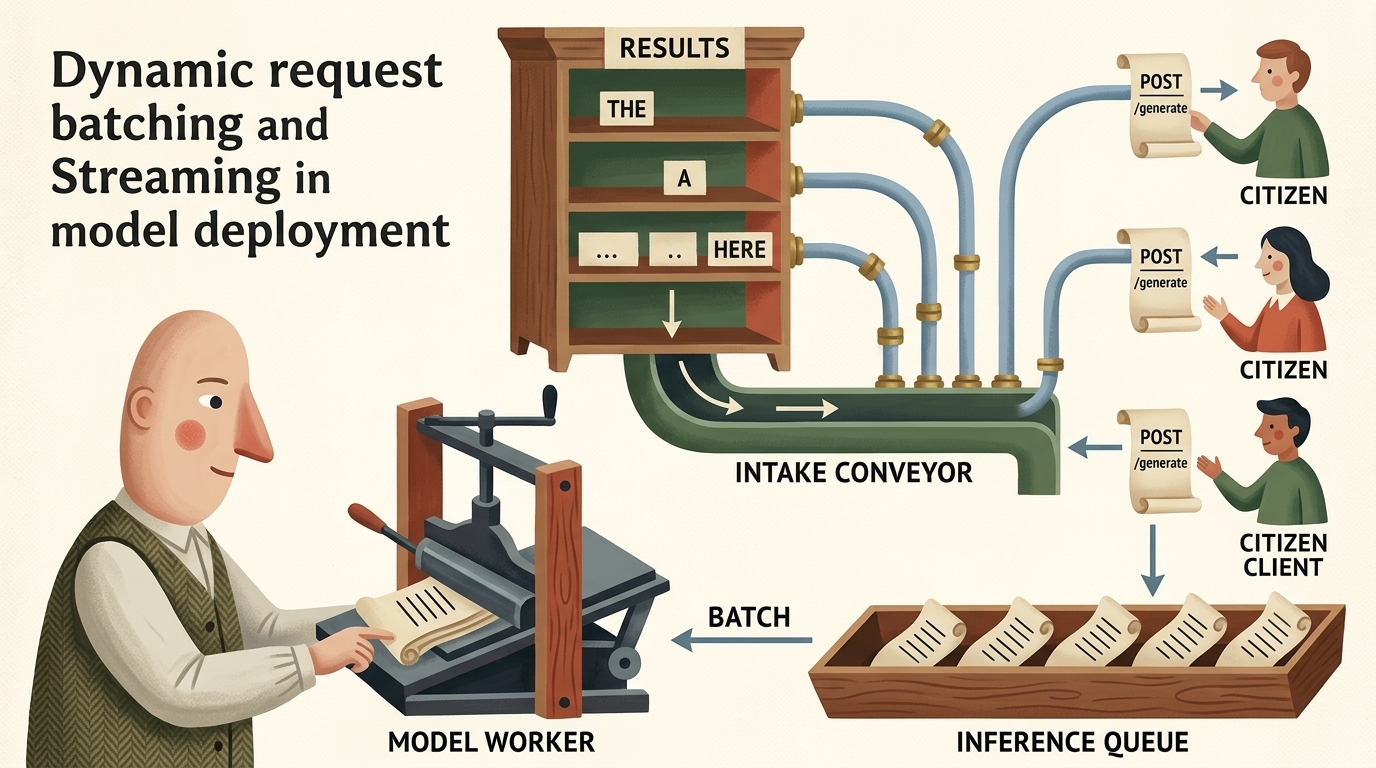
3.1 The Dynamic Batching Mechanism
To maximize accelerator efficiency, production servers implement Dynamic Batching. An asynchronous queue collects incoming client requests. A background model worker dequeues requests up to a maximum batch capacity $B_{\max}$, or triggers early if a maximum queue wait timeout $\tau_{\text{batch}}$ expires:
$$ B = \min\left( B_{\max}, \quad \text{queue.size}() \right) \quad \text{when } t - t_{\text{arrival}} \ge \tau_{\text{batch}} $$
The overall latency observed by an individual client $L(B)$ is the sum of queuing wait time and GPU execution time:
$$ L(B) = W_{\text{queue}}(B) + L_{\text{compute}}(B) $$
While $W_{\text{queue}}(B)$ increases with larger batch limits, $L_{\text{compute}}(B)$ scales sub-linearly on GPUs up to hardware saturation, substantially increasing overall system throughput:
$$ \text{Throughput}(B) = \frac{B}{L_{\text{compute}}(B)} $$
The code below implements an asynchronous dynamic batching server where concurrent client requests are gathered into batches via an asyncio.Queue, executed in a single batched tensor forward pass, and their results are resolved back to individual client futures:
import asyncio
from dataclasses import dataclass
from typing import Any
import torch
@dataclass
class QueueItem:
input_tensor: torch.Tensor
future: asyncio.Future
class DynamicBatcher:
def __init__(self, model: torch.nn.Module, max_batch_size: int = 16, max_wait_time: float = 0.005):
self.model = model
self.max_batch_size = max_batch_size
self.max_wait_time = max_wait_time
self.queue: asyncio.Queue[QueueItem] = asyncio.Queue()
self.worker_task = asyncio.create_task(self._batch_worker())
async def predict(self, x: torch.Tensor) -> torch.Tensor:
# Enqueue request and await dedicated response future
loop = asyncio.get_running_loop()
item = QueueItem(input_tensor=x, future=loop.create_future())
await self.queue.put(item)
return await item.future
async def _batch_worker(self):
while True:
first_item = await self.queue.get()
batch = [first_item]
deadline = asyncio.get_event_loop().time() + self.max_wait_time
# Accumulate requests until batch size or deadline is reached
while len(batch) < self.max_batch_size:
timeout = deadline - asyncio.get_event_loop().time()
if timeout <= 0:
break
try:
item = await asyncio.wait_for(self.queue.get(), timeout=timeout)
batch.append(item)
except asyncio.TimeoutError:
break
# 1. Collate individual tensors into a single hardware batch
batch_inputs = torch.cat([item.input_tensor for item in batch], dim=0)
# 2. Execute unified GPU forward pass
with torch.inference_mode():
outputs = self.model(batch_inputs)
# 3. Scatter slices back to corresponding client futures
for i, item in enumerate(batch):
item.future.set_result(outputs[i:i+1])
3.2 Asynchronous Token Streaming with Server-Sent Events (SSE)
For autoregressive large language models or iterative diffusion schedulers, waiting for the entire sequence generation to finish before returning any response ruins the user experience. By streaming individual tokens back to the client as they are sampled, we reduce the perceived latency from the full generation time down to the Time to First Token (TTFT).
In FastAPI, streaming is achieved using StreamingResponse wrapping an asynchronous Python generator:
from fastapi.responses import StreamingResponse
import asyncio
async def token_generator(prompt: str):
# Simulated autoregressive token generation stream
tokens = ["The", " model", " predicts", " a", " healthy", " tissue", " structure."]
for token in tokens:
await asyncio.sleep(0.04) # Simulate inter-token generation time
yield f"data: {token}\n\n"
@app.get("/stream-generate")
async def stream_generate(prompt: str):
return StreamingResponse(
token_generator(prompt),
media_type="text/event-stream"
)
4. Inference Acceleration Techniques: Precision, Quantization, and Memory Layouts
Running models in production with default 32-bit floating point (torch.float32) arithmetic wastes compute throughput and exhausts accelerator memory bandwidth.
4.1 Reduced Precision: FP16 and BF16
Modern GPU tensor cores (NVIDIA Volta, Ampere, Hopper, Blackwell) achieve orders-of-magnitude higher floating-point throughput when executing half-precision matrix multiplications:
| Floating-Point Format | Sign Bits | Exponent Bits | Mantissa (Fraction) Bits | Dynamic Range ($10^{\pm x}$) | Precision (Decimal Digits) |
|---|---|---|---|---|---|
| IEEE FP32 | 1 | 8 | 23 | $\approx 10^{\pm 38}$ | $\approx 7.2$ |
| IEEE FP16 | 1 | 5 | 10 | $\approx 10^{\pm 5}$ | $\approx 3.3$ |
| Bfloat16 (BF16) | 1 | 8 | 7 | $\approx 10^{\pm 38}$ | $\approx 2.1$ |
In inference mode, gradients are not computed, which eliminates the need for dynamic loss scaling. Casting model weights to torch.float16 or torch.bfloat16 immediately reduces the model’s memory footprint by $50%$ and doubles memory-bandwidth transfer rates:
# Cast model weights to half-precision
model = model.to(device=device, dtype=torch.bfloat16)
# Inference with autocast
with torch.inference_mode():
with torch.autocast(device_type=device.type, dtype=torch.bfloat16):
predictions = model(input_tensor.to(dtype=torch.bfloat16))
4.2 Quantization Spectrum: PTQ vs. QAT
Quantization maps continuous 32-bit or 16-bit floating-point tensors into low-bit discrete integers (typically 8-bit int8 or 4-bit int4):
$$ q = \text{round}\left( \frac{x}{S} \right) + Z $$
where $S \in \mathbb{R}^+$ is the arbitrary scale factor and $Z \in \mathbb{Z}$ is the zero-point offset.
flowchart TD
Q_TECH["Model Quantization Techniques"]
Q_TECH --> PTQ["Post-Training Quantization (PTQ)<br/>No retraining required; calibration set determines scale S and zero-point Z"]
Q_TECH --> QAT["Quantization-Aware Training (QAT)<br/>Simulates low-bit roundoff errors via fake-quantization during fine-tuning"]
PTQ --> DYN["Dynamic PTQ: Activations quantized dynamically at runtime"]
PTQ --> STAT["Static PTQ: Scale & Zero-point pre-calibrated with representative dataset"]
style Q_TECH fill:#1a1a2e,stroke:#4cc9f0,stroke-width:2px,color:#fff
style PTQ fill:#16213e,stroke:#52b788,stroke-width:1px,color:#fff
style QAT fill:#16213e,stroke:#f77f00,stroke-width:1px,color:#fff
style DYN fill:#0f3460,stroke:#52b788,stroke-width:1px,color:#fff
style STAT fill:#0f3460,stroke:#52b788,stroke-width:1px,color:#fff
For large language models and vision transformers, 4-bit weight quantization (such as AWQ or GPTQ) and 1-bit binary representations (BitNet $b1.58$) allow billion-parameter models to execute on consumer-grade hardware by drastically lowering HBM memory-bandwidth bottlenecks.
4.3 Memory Layout: Channels-Last for Convolutions
By default, PyTorch allocates 4D convolutional image tensors in contiguous NCHW order (Batch, Channel, Height, Width). However, modern x86 CPU AVX-512 vector units and NVIDIA Tensor Cores execute convolutions significantly faster when memory is organized in NHWC format, referred to in PyTorch as torch.channels_last:
# Convert convolutional model and inputs to channels-last layout
model = model.to(memory_format=torch.channels_last)
input_tensor = input_tensor.to(memory_format=torch.channels_last)
In torch.channels_last, adjacent elements in physical RAM represent different channels of the exact same pixel, enabling hardware vector registers to perform full dot products across the channel dimension with zero strided memory gathers.
5. Model Graph Capture & Export: From Python Code to Static Graphs
Deploying PyTorch models into high-performance, non-Python environments requires capturing the model’s dynamic computational graph into a serialized representation.
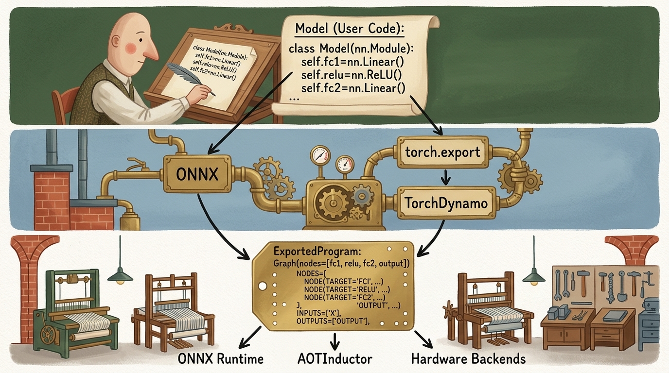
5.1 The Evolution: TorchScript vs. Modern torch.export
Historically, PyTorch provided TorchScript (torch.jit.trace and torch.jit.script) to serialize models into a Python-independent intermediate format. However, TorchScript suffered from severe limitations:
torch.jit.traceblindly followed a single execution path with dummy inputs, silently ignoring data-dependentifconditions and loops.torch.jit.scriptattempted to parse a subset of Python syntax into an AST, frequently failing on modern Python idioms, type annotations, and dynamic third-party libraries.
In PyTorch 2.x+, the official graph capture mechanism is torch.export. Unlike TorchScript, torch.export:
- Produces an exact, sound computational graph representing PyTorch’s ATen operator set.
- Captures dynamic dimensions cleanly using explicit symbolic shapes (
torch.export.Dim). - Guarantees that any unsupported dynamic construct causes an explicit export-time error rather than producing a silently corrupted graph.
The code below exports a multi-layer neural network using torch.export, specifying a dynamic batch size dimension so that the exported graph is valid for arbitrary batch inputs at runtime:
import torch
class Classifier(torch.nn.Module):
def __init__(self):
super().__init__()
self.fc1 = torch.nn.Linear(64, 32)
self.relu = torch.nn.ReLU()
self.fc2 = torch.nn.Linear(32, 2)
def forward(self, x: torch.Tensor) -> torch.Tensor:
return self.fc2(self.relu(self.fc1(x)))
model = Classifier().eval()
sample_input = (torch.randn(1, 64),)
# 1. Define symbolic dynamic dimensions for flexible serving batch sizes
batch_dim = torch.export.Dim("batch_size", min=1, max=128)
dynamic_shapes = {"x": {0: batch_dim}}
# 2. Capture sound graph representation into an ExportedProgram
exported_program: torch.export.ExportedProgram = torch.export.export(
model,
args=sample_input,
dynamic_shapes=dynamic_shapes
)
# Inspect the captured ATen graph nodes
print(exported_program.graph)
The resulting ExportedProgram is completely self-contained. It stores the mathematical computation graph, parameter buffers, input/output specifications, and validation guards, and can be saved to disk with torch.export.save(exported_program, "model.pt2").
5.2 Open Neural Network Exchange (ONNX) and ONNX Runtime
For cross-platform and multi-hardware deployment (e.g. running on Windows DirectML, Intel OpenVINO, or NVIDIA TensorRT without a PyTorch runtime), ONNX is the global industry standard.
In modern PyTorch, the ONNX exporter is integrated directly with TorchDynamo via the torch.onnx.export API:
import torch
model = Classifier().eval()
dummy_input = torch.randn(1, 64)
# Export directly to ONNX binary format
torch.onnx.export(
model,
dummy_input,
"model.onnx",
export_params=True,
opset_version=17,
do_constant_folding=True,
input_names=["input"],
output_names=["output"],
dynamic_axes={
"input": {0: "batch_size"},
"output": {0: "batch_size"}
}
)
Once exported, high-performance C++ runtimes such as ONNX Runtime execute the serialized model across heterogenous hardware with hardware-specific execution providers:
import onnxruntime as ort
import numpy as np
# Initialize ONNX Runtime inference session with CUDA acceleration
session = ort.InferenceSession("model.onnx", providers=["CUDAExecutionProvider", "CPUExecutionProvider"])
# Execute inference using standard NumPy buffers
input_name = session.get_inputs()[0].name
output_name = session.get_outputs()[0].name
data = np.random.randn(4, 64).astype(np.float32)
raw_outputs = session.run([output_name], {input_name: data})
6. Deep Dive into torch.compile & The Inductor Compiler Engine
Introduced in PyTorch 2.0, torch.compile delivers deep compiler-level optimizations while preserving the native, eager-mode Python developer experience. It requires zero code refactoring:
compiled_model = torch.compile(model, mode="max-autotune")
Underneath this simple API call lies a sophisticated three-tier compiler subsystem:
flowchart TD
USER_CODE["Python User Code (nn.Module / Functions)"]
subgraph T1 ["Tier 1: Graph Capture"]
DYNAMO["TorchDynamo (PEP 523 Frame Hook)<br/>Inspects Python CPython bytecode & evaluates guards"]
end
subgraph T2 ["Tier 2: Intermediate Representation & Autograd"]
AOT["AOTAutograd<br/>Decomposes complex operators into ~250 Core ATen ops"]
end
subgraph T3 ["Tier 3: Backend Code Generation"]
INDUCTOR["TorchInductor Compiler"]
TRITON["OpenAI Triton Kernels (NVIDIA / AMD GPUs)"]
CPP["C++ OpenMP Vectorized Code (x86 / ARM CPUs)"]
INDUCTOR --> TRITON
INDUCTOR --> CPP
end
USER_CODE --> DYNAMO
DYNAMO --> AOT
AOT --> INDUCTOR
style USER_CODE fill:#1a1a2e,stroke:#4cc9f0,stroke-width:2px,color:#fff
style T1 fill:#16213e,stroke:#52b788,stroke-width:1px,color:#fff
style T2 fill:#1a3a2a,stroke:#f77f00,stroke-width:1px,color:#fff
style T3 fill:#2b1b22,stroke:#e63946,stroke-width:2px,color:#fff
6.1 The Three Subsystems of torch.compile
- TorchDynamo (Frontend): Uses the Python C-API frame evaluation hook (
PEP 523) to intercept execution before bytecode is executed. It analyzes Python bytecode, extracts pure tensor operations into an FX computational graph, and installs Guards. Guards verify that assumptions about tensor dtypes, dimensions, and global variables remain true. If a guard fails at runtime, TorchDynamo falls back to standard Python execution. - AOTAutograd (Middle-tier): Decomposes thousands of high-level PyTorch APIs into approximately 250 primitive, functional Core ATen operations, eliminating side-effects and standardizing mathematical semantics.
- TorchInductor (Backend): The default deep learning compiler for PyTorch. Instead of relying on pre-compiled CUDA kernel libraries (like cuDNN or cuBLAS) for every individual operator, Inductor synthesizes custom OpenAI Triton code for GPUs and C++ with SIMD vector extensions for CPUs.
6.2 The Power of Operator Fusion (Eliminating the Memory Wall)
Why does torch.compile produce dramatic speedups on GPUs?
On modern accelerators, the theoretical compute throughput (TFLOPs) scales far faster than the memory bandwidth between High Bandwidth Memory (HBM/DRAM) and on-chip SRAM caches. In eager PyTorch, evaluating a sequential chain of point-wise operators:
$$ y = \text{GELU}(W x + b) $$
forces the accelerator to:
- Load $W$ and $x$ from HBM, compute matrix multiplication, and write the intermediate tensor back to HBM.
- Load the intermediate tensor from HBM into SRAM, add bias $b$, and write the result back to HBM.
- Load the biased result from HBM into SRAM, compute the non-linear GELU activation, and write the final result back to HBM.
This constant round-tripping across the memory bus saturates memory bandwidth, leaving GPU tensor cores starved for work. TorchInductor fuses these contiguous operations into a single custom Triton GPU kernel. The bias addition and GELU activation execute entirely inside GPU registers while the tensor data resides in on-chip SRAM, requiring only a single write-back to main memory.
6.3 Diagnosing and Fixing Graph Breaks
A Graph Break occurs when TorchDynamo encounters a Python construct that cannot be traced into an FX graph (for example, printing to stdout, invoking an unsupported C-extension, or evaluating a data-dependent conditional statement on tensor elements like if tensor.item() > 0:).
When a graph break occurs, TorchDynamo is forced to split the execution into two separate compiled subgraphs, dropping back into the slow Python CPython interpreter in between:
$$\text{Graph 1 (Compiled)} \longrightarrow \text{Python Interpreter Break} \longrightarrow \text{Graph 2 (Compiled)}$$
To diagnose graph breaks in production code, PyTorch provides dedicated diagnostic utilities:
import torch
# Diagnostic tool to explain why graph breaks occur
explanation = torch._dynamo.explain(model, sample_input)
print(f"Graph break count: {explanation.graph_break_count}")
print(f"Break reasons: {explanation.break_reasons}")
7. Execution Profiling with torch.profiler
Before optimizing a production service, engineers must profile the running workload to locate the true architectural bottlenecks: is execution compute-bound, memory-bandwidth bound, or dominated by CPU-side framework overheads?
The code below configures torch.profiler.profile to capture CPU and CUDA activities, track GPU memory allocations, and export execution traces in Chrome Trace Event format:
import torch
import torchvision.models as models
device = torch.device("cuda" if torch.cuda.is_available() else "cpu")
model = models.resnet18().to(device)
inputs = torch.randn(16, 3, 224, 224, device=device)
# Configure the PyTorch profiler
with torch.profiler.profile(
activities=[
torch.profiler.ProfilerActivity.CPU,
torch.profiler.ProfilerActivity.CUDA,
],
record_shapes=True,
profile_memory=True,
with_stack=True
) as prof:
# Warmup pass
model(inputs)
torch.cuda.synchronize() if torch.cuda.is_available() else None
# Profiling target iteration
with torch.profiler.record_function("production_inference_forward"):
outputs = model(inputs)
torch.cuda.synchronize() if torch.cuda.is_available() else None
# Print top operators sorted by total GPU execution time
print(prof.key_averages().table(sort_by="cuda_time_total", row_limit=10))
# Export complete execution trace for interactive visualization in chrome://tracing or Perfetto
prof.export_chrome_trace("production_profile_trace.json")
Inspecting the resulting trace in chrome://tracing or Perfetto reveals:
- GPU Kernel Concurrency: Whether the GPU is continuously saturated or experiencing bubbles due to CPU scheduling delays.
- Memory Allocation Spikes: Memory allocation and deallocation events that trigger expensive CUDA memory allocator locks.
- Kernel Launch Overhead: The delay between a CPU dispatch call and the actual start of execution on the GPU stream.
8. Python-Free Zero-Overhead Serving: LibTorch (C++)
While Python is the preeminent language for deep learning research, high-performance production systems often eliminate Python entirely from the serving path. Environments such as autonomous vehicle control systems, high-frequency trading platforms, robotic systems running ROS 2, and game engines require:
- Deterministic Latency: Complete freedom from Python garbage collection pauses.
- True Multithreaded Concurrency: Total bypass of the Python Global Interpreter Lock (GIL).
- Minimal Memory Footprint: Running lean binaries on systems without a Python runtime or package manager installed.
PyTorch provides LibTorch, a pure C++ library containing the complete ATen tensor library and torch::nn module interfaces.
8.1 Loading and Executing Exported Models in C++
Models exported from Python (via AOTInductor or TorchScript) can be loaded directly inside a C++ application:
#include <torch/script.h> // Or torch/all.h for full LibTorch API
#include <iostream>
#include <memory>
int main(int argc, const char* argv[]) {
if (argc != 2) {
std::cerr << "Usage: inference_server <path-to-exported-model>\n";
return -1;
}
// 1. Configure target execution device
torch::DeviceType device_type = torch::cuda::is_available() ? torch::kCUDA : torch::kCPU;
torch::Device device(device_type);
std::cout << "Executing inference on: " << (device.is_cuda() ? "CUDA GPU" : "Host CPU") << std::endl;
// 2. Deserialize model binary from disk into C++ runtime
torch::jit::script::Module module;
try {
module = torch::jit::load(argv[1]);
module.to(device);
module.eval();
} catch (const c10::Error& e) {
std::cerr << "Fatal error loading model binary: " << e.msg() << std::endl;
return -1;
}
// 3. Create input tensor directly using C++ ATen API
std::vector<torch::jit::IValue> inputs;
torch::Tensor input_tensor = torch::randn({1, 3, 224, 224}, device);
inputs.push_back(input_tensor);
// 4. Zero-overhead C++ forward execution
at::Tensor output = module.forward(inputs).toTensor();
std::cout << "Inference completed successfully. Output shape: " << output.sizes() << std::endl;
return 0;
}
8.2 Building with CMake
LibTorch integrates seamlessly with standard C++ build systems using CMake:
cmake_minimum_required(VERSION 3.18 FATAL_ERROR)
project(production_inference_service CXX)
set(CMAKE_CXX_STANDARD 17)
find_package(Torch REQUIRED)
add_executable(inference_server main.cpp)
target_link_libraries(inference_server "${TORCH_LIBRARIES}")
set_property(TARGET inference_server PROPERTY CXX_STANDARD 17)
By compiling against LibTorch, the resulting native binary runs with zero Python dependency, achieving predictable microsecond-level latency and full integration with C++ multi-threaded thread pools.
9. Mobile & Edge Deployment: ExecuTorch
Deploying deep learning models to battery-powered, memory-constrained edge hardware (smartphones, IoT sensors, wearable medical devices) requires a radical departure from server-scale runtimes. LibTorch and standard PyTorch runtimes have binary sizes exceeding $50\text{–}100\text{ MB}$ and allocate dynamic memory continuously.
PyTorch 2.x introduces ExecuTorch, a modern edge runtime engineered from first principles for on-device AI.
flowchart TD
E_PY["Python PyTorch 2.x Model"] --> E_EXP["torch.export (Sound Graph Capture)"]
E_EXP --> E_OPT["ExecuTorch Ahead-Of-Time Compiler<br/>Memory planning, operator lowering & quantization"]
E_OPT --> E_BIN["Standalone .pte Program Binary"]
subgraph Runtimes ["Lightweight On-Device ExecuTorch Runtime (< 2 MB)"]
direction TB
E_BIN --> B1["XNNPACK Backend (ARM / x86 CPUs)"]
E_BIN --> B2["CoreML Backend (Apple Neural Engine)"]
E_BIN --> B3["Qualcomm QNN Backend (Snapdragon NPU)"]
E_BIN --> B4["Vulkan / Metal GPU Backends"]
end
style E_PY fill:#1a1a2e,stroke:#4cc9f0,stroke-width:2px,color:#fff
style E_EXP fill:#16213e,stroke:#52b788,stroke-width:1px,color:#fff
style E_OPT fill:#1a3a2a,stroke:#f77f00,stroke-width:1px,color:#fff
style E_BIN fill:#2b1b22,stroke:#e63946,stroke-width:2px,color:#fff
style Runtimes fill:#0f3460,stroke:#4cc9f0,stroke-width:2px,color:#fff
Key Architectural Pillars of ExecuTorch:
- Ultra-Lean Binary Size: The core ExecuTorch C++ runtime fits within a tiny footprint (under $2\text{ MB}$ stripped), enabling integration into strict mobile apps and embedded firmware.
- Zero Dynamic Allocation at Runtime: ExecuTorch executes an Ahead-Of-Time Memory Planner that pre-allocates a static memory arena for all intermediate activations. During inference, zero heap allocations (
malloc/new) occur, eliminating latency jitter and preventing out-of-memory crashes on constrained operating systems. - Hardware Acceleration Backends: Seamlessly delegates subgraphs to specialized edge processors:
- XNNPACK: Highly optimized SIMD kernels for ARM Cortex-A/M and x86 CPUs.
- CoreML: Direct hardware access to Apple Silicon Neural Engine (ANE).
- Qualcomm QNN: Native acceleration on Snapdragon Hexagon NPUs.
10. Production Decision Framework: Choosing the Right Deployment Stack
Navigating the landscape of deep learning deployment technologies requires balancing hardware constraints, request concurrency, latency SLAs, and infrastructure complexity.
| Deployment Target | Primary Stack | Strengths | Trade-offs & Limitations | Ideal Use Case |
|---|---|---|---|---|
| Interactive Research & HITL | Gradio / Streamlit | Zero-boilerplate UI, rapid parameter exploration | Single-client focus, high per-request overhead | Medical diagnostic validation, stakeholder demonstrations |
| Asynchronous Web Microservice | FastAPI + Uvicorn + Dynamic Batching | Python-native, async concurrency, easy scaling | Python GIL overhead, manual queue tuning required | Mid-scale internal APIs, microservice integrations |
| High-Throughput Foundation Serving | Triton Inference Server / vLLM / TGI | PagedAttention, continuous batching, multi-model GPU sharing | Complex Docker orchestration, higher deployment friction | Enterprise LLMs, multi-tenant cloud serving |
| High-Performance Python Production | torch.compile (Inductor) | Native PyTorch, automatic Triton kernel fusion, zero model rewrite | Initial compilation overhead on startup, potential graph breaks | High-throughput computer vision and NLP model serving |
| Cross-Platform Enterprise Systems | ONNX + ONNX Runtime | Broad vendor support (TensorRT, OpenVINO, DirectML), standard format | Export limitations for complex dynamic control flow | Heterogeneous enterprise hardware, legacy C#/Java/Go backends |
| Zero-Overhead Native Serving | LibTorch (C++) | Microsecond deterministic latency, no GIL, C++ ecosystem embedding | Requires C++ build tooling, manual memory management | Autonomous vehicles, robotics (ROS 2), game engines |
| Resource-Constrained Edge & Mobile | ExecuTorch | Sub-2MB runtime, zero dynamic allocation, NPU/DSP hardware delegates | Limited operator coverage, strict export pipeline | iOS/Android mobile apps, embedded wearables, IoT sensors |
The Production Architecture Decision Tree
flowchart TD
START["What is your primary deployment target?"]
START --> D1{"Target Platform?"}
D1 -->|"Mobile / Embedded / IoT"| DEC_MOB["ExecuTorch<br/>Static memory planning and NPU acceleration"]
D1 -->|"Robotics / Game Engine / Zero-GIL"| DEC_CPP["LibTorch C++<br/>Deterministic microsecond execution"]
D1 -->|"Cloud Server / Enterprise Service"| D2{"Model Type and Concurrency?"}
D2 -->|"High-Throughput Autoregressive LLM"| DEC_LLM["vLLM / TensorRT-LLM<br/>Continuous batching and PagedAttention"]
D2 -->|"Standard Vision / Tabular / Audio"| D3{"Hardware Heterogeneity?"}
D3 -->|"NVIDIA GPU Dedicated Cloud"| DEC_COMP["PyTorch 2.x and torch.compile<br/>FastAPI async service with dynamic batching"]
D3 -->|"Cross-Platform (Intel / AMD / ARM / ONNX)"| DEC_ONNX["ONNX Runtime<br/>Hardware-specific execution providers"]
style START fill:#1a1a2e,stroke:#4cc9f0,stroke-width:2px,color:#fff
style DEC_MOB fill:#2b1b22,stroke:#e63946,stroke-width:2px,color:#fff
style DEC_CPP fill:#16213e,stroke:#52b788,stroke-width:1px,color:#fff
style DEC_LLM fill:#1a3a2a,stroke:#f77f00,stroke-width:1px,color:#fff
style DEC_COMP fill:#0f3460,stroke:#4cc9f0,stroke-width:2px,color:#fff
style DEC_ONNX fill:#16213e,stroke:#52b788,stroke-width:2px,color:#fff
11. Exercises & Conceptual Verification
To solidify your mastery of deep learning deployment systems, implement solutions to the following engineering challenges:
-
Dynamic Batching Latency Analysis:
- In a production server with maximum batch size $B_{\max} = 32$ and timeout $\tau_{\text{batch}} = 10\text{ ms}$, suppose request arrival follows a Poisson distribution with mean arrival rate $\lambda = 500\text{ requests/sec}$.
- Calculate the average batch size $\mathbb{E}[B]$ formed by the worker.
- Formulate the expected wait time $W_{\text{queue}}$ experienced by the first request entering an empty queue.
-
Benchmarking Eager vs.
torch.compile:- Take a standard ResNet-50 or Vision Transformer architecture.
- Profile the forward pass execution time across 100 iterations under eager mode vs.
torch.compile(mode="reduce-overhead"). - Measure the GPU memory bandwidth utilization and identify the specific fused operators generated by TorchInductor.
-
Diagnosing Graph Breaks:
- Construct a custom
nn.Modulecontaining a Pythonprint()statement and a dynamic tensor-dependent slicex[:x.shape[0] // 2]. - Run
torch._dynamo.explain()to identify the exact line triggering the graph break. - Refactor the module using purely functional tensor operations so that
torch.compilecaptures a single unified computational graph without any breaks.
- Construct a custom
12. Conclusion & Summary
In this final chapter of Part 2, we completed the journey from neural network theory and distributed training to full-scale production deployment:
- Serving Paradigms: We contrasted human-in-the-loop rapid interfaces (Gradio) with high-concurrency asynchronous microservices (FastAPI), establishing patterns to protect the Python asyncio event loop from blocking tensor operations.
- Dynamic Batching & Streaming: We analyzed how asynchronous queues aggregate discrete client requests into high-throughput hardware batches, and how Server-Sent Events stream tokens incrementally to minimize Time to First Token (TTFT).
- Inference Optimization: We reviewed the precision and quantization spectrum (FP16, BF16, INT8, INT4, 1-bit) and the memory bandwidth advantages of
channels_lasttensor formatting. - Modern Graph Export: We traced the transition from legacy TorchScript to sound, whole-graph capture via
torch.exportand cross-platform execution via ONNX and ONNX Runtime. - Compiler Acceleration: We dissected the three-tier architecture of
torch.compile(TorchDynamo, AOTAutograd, TorchInductor) and explored how operator fusion overcomes the GPU memory bandwidth wall. - Non-Python Runtimes: We evaluated zero-overhead deterministic C++ serving via LibTorch and lean, zero-allocation mobile deployment via ExecuTorch.
With these production foundations established, you possess the full-stack engineering toolkit to design, train, scale, compile, and deploy state-of-the-art deep learning systems across any industrial computing infrastructure.
Hoş Geldiniz
Derin Öğrenme Notları
Deep Learning Specialization kapsamında alınan notlar
Andrew Ng & Eddy Shyu tarafından
Stanford Üniversitesi & DeepLearning.AI
İşlenen Dersler
| # | Ders | Odak |
|---|---|---|
| 1 | Sinir Ağları ve Derin Öğrenme | Lojistik regresyon sinir ağı olarak, sığ & derin ağlar, ileri/geri yayılım |
| 2 | Derin Sinir Ağlarını Geliştirme | Hiperparametre ayarı, düzenlileştirme (Dropout, BatchNorm), optimizasyon (Momentum, Adam), Xavier/He başlatma |
| 3 | Makine Öğrenmesi Projelerini Yapılandırma | Train/dev/test ayrımı, hata analizi, transfer öğrenmesi, uçtan uca derin öğrenme |
| 4 | Konvolüsyonel Sinir Ağları | CNNs, kenar tespiti, klasik & modern mimariler (LeNet, AlexNet, VGG, ResNet, Inception, MobileNet, EfficientNet), nesne tespiti (YOLO), yüz tanıma (FaceNet, Siamese), neural style transfer, U-Net |
| 5 | Sequence Modelleri | RNNs, GRUs, LSTMs, kelime gömmeleri (Word2Vec, GloVe), dikkat mekanizması, Transformer, konuşma tanıma, müzik sentezi, makine çevirisi, sohbet robotları |
— emreaslan —
İçerik
Hoş geldiniz — Machine Learning notları.
∴
Machine Learning Specialization kursunu tamamlarken aldığım detaylı notlar — temel kavramlardan ileri algoritmalara, her konu kendi cümlelerimle açıklanmış ve kod örnekleriyle pekiştirilmiş.
Stanford Üniversitesi & DeepLearning.AI
— emreaslan —
Denetimli ve Denetimsiz Makine Öğrenmesi (Supervised and Unsupervised Machine Learning)
Giriş (Introduction)
Makine öğrenmesi (machine learning), yapay zekânın bir dalı olup sistemlerin açık bir şekilde programlanmadan öğrenmesine, tahminler yapmasına veya kararlar almasına olanak tanır. İki ana makine öğrenmesi türü Denetimli Öğrenme (Supervised Learning) ve Denetimsiz Öğrenmedir (Unsupervised Learning). Aşağıda, bu iki türün özelliklerini, alt alanlarını ve görsel bir temsilini bulabilirsiniz.
graph TD
A[Makine Öğrenmesi] --> B[Denetimli Öğrenme]
A --> C[Denetimsiz Öğrenme]
B --> D[Regresyon]
B --> E[Sınıflandırma]
C --> F[Kümeleme]
C --> G[Birliktelik]
C --> H[Boyut İndirgeme]
Denetimli Öğrenme (Supervised Learning)
Denetimli öğrenme, modelin etiketlenmiş veriler (labeled data) üzerinde eğitildiği bir makine öğrenmesi türüdür. Etiketlenmiş veri, her girdi için karşılık gelen bir çıktının (veya hedefin) önceden sağlanmış olduğu anlamına gelir. Modelin amacı, girdiler ve çıktılar arasındaki ilişkiyi öğrenerek yeni, görülmemiş veriler için tahminler yapabilmektir.
Temel Özellikler (Key Characteristics)
- Girdi ve Çıktı: Eğitim verisi, hem girdi özelliklerini (X) hem de hedef etiketleri (Y) içerir.
- Amaç: Belirli bir girdi (X) için çıktıyı (Y) tahmin etmek.
Alt Alanlar (Subfields)
- Regresyon (Regression): Sürekli değerlerin tahmin edilmesi (örneğin, daire büyüklüğüne göre kira fiyatlarının tahmin edilmesi).
- Sınıflandırma (Classification): Girdilerin ayrık kategorilere atanması (örneğin, kanserin iyi huylu veya kötü huylu olarak teşhis edilmesi).
Örnek: Regresyon (Regression)
- Senaryo: Daire büyüklüğüne (m²) göre kira fiyatlarının tahmin edilmesi.
- Detaylar:
- Girdi özellikleri (X): Daire büyüklüğü, oda sayısı, mahalle vb.
- Hedef değişken (Y): Kira fiyatı (örneğin, aylık $).
- Modelin Görevi: Daire özellikleri ile kira fiyatları arasındaki ilişkiyi öğrenmek ve yeni bir daire için kira fiyatını tahmin etmek.
Örnek: Sınıflandırma (Classification)
- Senaryo: Kanser teşhisi (örneğin, iyi huylu veya kötü huylu tümör).
- Detaylar:
- Girdi özellikleri (X): Tümör boyutu, doku, hücre şekli gibi ölçümler.
- Hedef değişken (Y): Sınıf etiketi (örneğin, “İyi Huylu” veya “Kötü Huylu”).
- Modelin Görevi: Girdi özelliklerine dayanarak yeni bir tümörü iyi huylu veya kötü huylu olarak sınıflandırmak.
Denetimsiz Öğrenme (Unsupervised Learning)
Denetimsiz öğrenme, etiketlenmemiş veriler (unlabeled data) ile ilgilenir. Model, önceden tanımlanmış herhangi bir etiket veya hedef olmadan veri içindeki örüntüleri, yapıları veya ilişkileri bulmaya çalışır. Genellikle keşifsel veri analizi (exploratory data analysis) için kullanılır.
Temel Özellikler (Key Characteristics)
- Yalnızca Girdi: Veri, yalnızca girdi özelliklerini (X) içerir, hedef etiketleri (Y) yoktur.
- Amaç: Verideki gizli örüntüleri veya gruplaşmaları keşfetmek.
Alt Alanlar (Subfields)
- Kümeleme (Clustering): Benzer veri noktalarını kümeler halinde gruplama (örneğin, müşteri segmentasyonu).
- Boyut İndirgeme (Dimensionality Reduction): Önemli bilgileri koruyarak veri setindeki özellik sayısını azaltma (örneğin, PCA).
- Birliktelik (Association): Büyük veri setlerinde değişkenler arasındaki ilişkileri veya birliktelikleri keşfetme (örneğin, sepet analizi).
Örnek: Kümeleme (Clustering)
- Senaryo: Hedefli pazarlama için müşterilerin gruplandırılması.
- Detaylar:
- Girdi özellikleri (X): Müşteri yaşı, geliri, satın alma geçmişi, konumu vb.
- Önceden tanımlanmış etiketler (Y) yoktur.
- Modelin Görevi: Müşteri kümelerini belirlemek (örneğin, “Yüksek harcamacılar,” “Bütçe bilincine sahip alıcılar”).
Örnek: Boyut İndirgeme (Dimensionality Reduction)
- Senaryo: Yüksek boyutlu verilerin görselleştirilmesi.
- Detaylar:
- 100’den fazla özelliğe sahip bir veri setiniz olduğunu düşünün (örneğin, bir fabrikadan alınan sensör verileri).
- Boyut indirgeme (örneğin, PCA), daha kolay görselleştirme için veriyi 2B veya 3B’ye indirgemeye yardımcı olur.
- Modelin Görevi: Karmaşıklığı azaltırken verinin önemli yapısını korumak.
Örnek: Birliktelik (Association)
- Senaryo: Ürün birlikteliklerini belirlemek için sepet analizi (market basket analysis).
- Detaylar:
- Girdi özellikleri (X): Birlikte satın alınan ürünleri gösteren işlem verileri.
- Önceden tanımlanmış etiketler (Y) yoktur.
- Modelin Görevi: “Bir müşteri ekmek alıyorsa, tereyağı alma olasılığı yüksektir” gibi kurallar belirlemek.
- Kullanım Alanı: Öneri sistemleri, envanter planlaması.
Karşılaştırma Tablosu (Comparison Table)
| Özellik | Denetimli Öğrenme | Denetimsiz Öğrenme |
|---|---|---|
| Veri Türü | Etiketlenmiş veri (X, Y) | Etiketlenmemiş veri (yalnızca X) |
| Amaç | Sonuçları tahmin etmek | Örüntüler veya yapılar bulmak |
| Temel Teknikler | Regresyon, Sınıflandırma | Kümeleme, Boyut İndirgeme, Birliktelik |
| Örnekler | Dolandırıcılık tespiti, Hisse senedi fiyat tahmini | Pazar segmentasyonu, Görüntü sıkıştırma |
Anahtar Çıkarımlar (Key Takeaways)
- Denetimli Öğrenme, etiketlenmiş veri gerektirir ve regresyon ile sınıflandırma gibi tahmin görevlerinde yaygın olarak kullanılır.
- Denetimsiz Öğrenme, etiketlenmemiş verilerle çalışır ve kümeleme veya boyut indirgeme yoluyla gizli örüntüleri bulmaya odaklanır.
- Her tekniğin belirli uygulamaları vardır ve probleme ile mevcut veriye göre seçilir.
- Lineer Regresyon ve Maliyet Fonksiyonu (Linear Regression and Cost Function)
Lineer Regresyon ve Maliyet Fonksiyonu (Linear Regression and Cost Function)
1. Giriş (Introduction)
Lineer regresyon (linear regression), makine öğrenimindeki temel algoritmalardan biridir. Özellikle girdi ve çıktı değişkenleri arasındaki ilişkinin doğrusal olduğu varsayıldığında, tahmine dayalı modelleme (predictive modeling) için yaygın olarak kullanılır. Temel amaç, tahmin edilen değerler ile gerçek değerler arasındaki hatayı en aza indiren en uygun doğruyu bulmaktır.
Neden Lineer Regresyon?
Lineer regresyon, birçok gerçek dünya uygulaması için basit ancak güçlüdür. Bazı yaygın kullanım alanları şunlardır:
- Ev fiyatlarını tahmin etmek — büyüklük, oda sayısı ve konum gibi özelliklere dayanarak.
- Maaşları tahmin etmek — deneyim, eğitim seviyesi ve sektöre göre.
- Trendleri anlamak — finans, sağlık ve ekonomi gibi çeşitli alanlarda.
Gerçek Dünya Örneği: Konut Fiyatları
Ev büyüklüğüne (metrekare cinsinden) dayanarak ev fiyatlarını tahmin etmeyi düşünelim. Basit bir doğrusal ilişki varsayılabilir: daha büyük evler daha yüksek fiyatlara sahip olma eğilimindedir. Bu varsayım, lineer regresyon modelimizin temelidir.
2. Matematiksel Gösterim (Mathematical Representation)
Basit bir lineer regresyon modeli, girdi $x$ (metrekare cinsinden ev büyüklüğü) ile çıktı $y$ (ev fiyatı) arasında doğrusal bir ilişki olduğunu varsayar. Şu şekilde gösterilir:
$$ h_θ(x) = \theta_0 + \theta_1 x $$
burada:
- $h_θ(x) $ tahmin edilen ev fiyatıdır.
- $ \theta_0 $ (kesim noktası - intercept) ve $\theta_1 $ (eğim - slope) modelin parametreleridir.
- $x$ ev büyüklüğüdür.
- $y$ gerçek ev fiyatıdır.
2.1 Lineer Modeli Anlamak
Peki bu denklem gerçekte ne anlama geliyor?
-
$\theta_0$ (kesim noktası - intercept): Büyüklüğü 0 m² olduğunda bir evin fiyatı.
-
$\theta_1$ (eğim - slope): Her ilave metrekare için ev fiyatındaki artış.
Örneğin, eğer:
-
$\theta_0 = 50,000$ ve $\theta_1 = 300$ ise,
-
100 m²’lik bir evin maliyeti: $ h_θ(100) = 50000 + 300 \cdot 100 = 80000 $
-
200 m²’lik bir evin maliyeti: $ h_θ(200) = 50000 + 300 \cdot 200 = 110000 $
Bu ilişkiyi bir regresyon doğrusu kullanarak görselleştirebiliriz.
3. Lineer Regresyonu Adım Adım Uygulama
Teorik kavramları daha net hale getirmek için, regresyon modelini Python kullanarak adım adım uygulayalım.
3.1 Gerekli Kütüphaneleri İçe Aktarma
import numpy as np
import matplotlib.pyplot as plt
import seaborn as sns
3.2 Örnek Veri Oluşturma
np.random.seed(42)
x = 50 + 200 * np.random.rand(100, 1) # Ev büyüklükleri m² cinsinden (50 ila 250)
y = 50000 + 300 * x + np.random.randn(100, 1) * 5000 # Gürültülü ev fiyatları
Burada, 100 örneklemli bir veri seti oluşturuyoruz:
-
$x$ ev büyüklüklerini temsil eder ($50$ ile $250$ m² arasında rastgele değerler).
-
$y$ ev fiyatlarını temsil eder, doğrusal bir ilişki izler ancak bir miktar gürültü (noise) içerir.
3.3 Veriyi Görselleştirme
plt.figure(figsize=(8,6))
sns.scatterplot(x=x.flatten(), y=y.flatten(), color='blue', alpha=0.6)
plt.xlabel('Ev Büyüklüğü (m²)')
plt.ylabel('Ev Fiyatı ($)')
plt.title('Ev Fiyatları ve Büyüklük')
plt.show()
3.4 Regresyon Doğrusunu Çizdirme
Maliyet fonksiyonuna geçmeden önce, verimize basit bir regresyon doğrusu yerleştirelim ve görselleştirelim.
Gerçek dünya uygulamalarında, bu parametreleri manuel olarak hesaplamayız. Bunun yerine, lineer regresyonu verimli bir şekilde gerçekleştirmek için scikit-learn gibi kütüphaneler kullanırız.
3.4.1 Eğimi Hesaplama ($\theta_1$)
theta_1 = np.sum((x - np.mean(x)) * (y - np.mean(y))) / np.sum((x - np.mean(x))**2)
Burada, eğimi ($\theta_1$) en küçük kareler yöntemi (least squares method) ile hesaplıyoruz.
3.4.2 Kesim Noktasını Hesaplama ($\theta_0$)
theta_0 = np.mean(y) - theta_1 * np.mean(x)
Bu, kesim noktasını ($\theta_0$) hesaplar ve regresyon doğrumuzun verinin ortalamasından geçmesini sağlar.
3.5 Regresyon Doğrusunu Çizdirme
y_pred = theta_0 + theta_1 * x # Tahmin edilen değerleri hesapla
plt.figure(figsize=(8,6))
sns.scatterplot(x=x.flatten(), y=y.flatten(), color='blue', alpha=0.6, label='Gerçek Veriler')
plt.plot(x, y_pred, color='red', linewidth=2, label='Regresyon Doğrusu')
plt.xlabel('Ev Büyüklüğü (m²)')
plt.ylabel('Ev Fiyatı ($)')
plt.title('Lineer Regresyon Modeli: Ev Fiyatları ve Büyüklük')
plt.legend()
plt.show()
3.6 Regresyon Doğrusunun Yorumlanması
Peki, bu doğru bize ne anlatıyor?
✅ Eğer eğim $\theta_1$ pozitifse, daha büyük evler daha pahalıdır (beklendiği gibi).
✅ Eğer kesim noktası $\theta_0$ yüksekse, en küçük evlerin bile önemli bir taban fiyatı olduğu anlamına gelir.
✅ Doğrunun dikliği, fiyatın metrekare başına ne kadar arttığını gösterir.
4. Maliyet Fonksiyonu (Cost Function)
Modelimizin ne kadar iyi performans gösterdiğini ölçmek için maliyet fonksiyonunu (cost function) kullanırız. Lineer regresyon için en yaygın maliyet fonksiyonu Ortalama Karesel Hata (Mean Squared Error - MSE)’dir:
$$ J(\theta) = \frac{1}{2m} \sum (h_{\theta}(x_i) - y_i)^2 $$
burada:
- $ m $ eğitim örneklerinin sayısıdır (number of training examples).
- $ h_\theta(x_i) $ $ i.$ ev için tahmin edilen fiyattır.
- $ y_i $ gerçek fiyattır.
Kesikli çizgilerin her biri bir hatayı (error) gösterir. Yukarıdaki formülde, bunların toplamını yani $J(\theta)$’yı hesapladık.
Bu fonksiyon, tahmin edilen ve gerçek değerler arasındaki ortalama karesel farkı hesaplar ve büyük hataları daha fazla cezalandırır. Amaç, en iyi model parametrelerine ulaşmak için $J(\theta)$’yı en aza indirmektir (minimize etmektir).
4.1 Örnek: $\theta_1 = 0$ Varsayımı
Maliyet fonksiyonunun nasıl davrandığını göstermek için, $\theta_1 = 0$ olduğunu varsayalım, yani modelimiz yalnızca $\theta_0$’a bağlıdır. Dört x değeri ve y değerinden oluşan küçük bir veri seti kullanacağız:
| x değerleri | y değerleri |
|---|---|
| 1 | 2 |
| 2 | 4 |
| 3 | 6 |
| 4 | 8 |
$\theta_1 = 0$ varsaydığımız için hipotez fonksiyonumuz şu şekilde sadeleşir: $$h_{\theta}(x) = \theta_0 \cdot x $$
$\theta_0$’ın farklı değerlerini değerlendirecek ve karşılık gelen maliyet fonksiyonunu hesaplayacağız.
Durum 1: $\theta_0 = 1$
$\theta_0 = 1$ için tahmin edilen değerler:
$$ h_θ(x) = 1 \cdot x = [1, 2, 3, 4] $$
Hata değerleri:
$$ \text{error} = h_θ(x) - y = [1 - 2, 2 - 4, 3 - 6, 4 - 8] = [-1, -2, -3, -4] $$
Maliyet fonksiyonunu hesaplama:
$$ J(\theta_0 = 1) = \frac{1}{2m} \sum (h_{\theta}(x_i) - y_i)^2 $$
$$ J(1) = \frac{1}{8} ((-1)^2 + (-2)^2 + (-3)^2 + (-4)^2) = \frac{1}{8} (1 + 4 + 9 + 16) = \frac{30}{8} = 3.75 $$
Durum 2: $\theta_0 = 1.5$
$\theta_0 = 1.5$ için tahmin edilen değerler:
$$ h_θ(x) = 1.5 \cdot x = [1.5, 3, 4.5, 6] $$
Hata değerleri:
$$ \text{error} = [1.5 - 2, 3 - 4, 4.5 - 6, 6 - 8] = [-0.5, -1, -1.5, -2] $$
Maliyet fonksiyonunu hesaplama:
$$ J(1.5) = \frac{1}{8} ((-0.5)^2 + (-1)^2 + (-1.5)^2 + (-2)^2) $$
$$ J(1.5) = \frac{1}{8} (0.25 + 1 + 2.25 + 4) = \frac{7.5}{8} = 0.9375 $$
Durum 3: $\theta_0 = 2$ (Optimal Durum)
$\theta_0 = 2$ için tahmin edilen değerler gerçek değerlerle eşleşir:
$$ h_θ(x) = 2 \cdot x = [2, 4, 6, 8] $$
Hata değerleri:
$$ \text{error} = [2 - 2, 4 - 4, 6 - 6, 8 - 8] = [0, 0, 0, 0] $$
Maliyet fonksiyonunu hesaplama:
$$ J(2) = \frac{1}{8} ((0)^2 + (0)^2 + (0)^2 + (0)^2) = 0 $$
Karşılaştırma
Hesaplamalarımıza göre:
- $ J(1) = 3.75 $
- $ J(1.5) = 0.9375 $
- $ J(2) = 0 $
Beklendiği gibi, maliyet fonksiyonu $\theta_0 = 2$ olduğunda en aza iner ve bu değer veri setine mükemmel şekilde uyar. Bu değerden herhangi bir sapma daha yüksek bir maliyetle sonuçlanır.
Peki makine kaç kez deneyip doğru değeri bulabilir? Buna nasıl öğretebiliriz? Cevap bir sonraki konuda.
Gradient Descent
- Gradient Descent’e Giriş (Introduction to Gradient Descent)
- Gradient Descent’in Matematiksel Formülasyonu (Mathematical Formulation of Gradient Descent)
- Öğrenme Oranı (Learning Rate — $\alpha$)
- Gradient Descent Yakınsaması (Convergence)
- Yerel Minimum (Local Minimum) ve Global Minimum (Global Minimum)
Gradient Descent’e Giriş (Introduction to Gradient Descent)
Önceki bölümde, $\theta_1 = 0$ varsayımıyla farklı $\theta_0$ değerleri aldığımızda maliyet fonksiyonunun nasıl davrandığını keşfetmiştik (Görselleştirmeyi kolaylaştırmak için $\theta_1$’e sıfır verdik). Şimdi, $J(\theta)$ maliyet fonksiyonunu en aza indiren en iyi parametreleri bulmak için kullanılan bir optimizasyon algoritması olan Gradient Descent’i (Gradyan İnişi) tanıtıyoruz.
Hipotez fonksiyonumuz şu şekilde sadeleşir: $$h_{\theta}(x) = \theta_0 \cdot x $$
Gradient Descent, $\theta$ parametresini maliyet fonksiyonunu azaltan yönde adım adım güncelleyen yinelemeli (iterative) bir yöntemdir. Algoritma, farklı değerleri manuel olarak test etmek yerine $\theta_0$’ın optimal değerini verimli bir şekilde bulmamıza yardımcı olur.
Gradient Descent’in nasıl çalıştığını anlamak için veri kümemizi (dataset) hatırlayalım:
| x değerleri | y değerleri |
|---|---|
| 1 | 2 |
| 2 | 4 |
| 3 | 6 |
| 4 | 8 |
Tahminlerimiz $h_\theta(x) = \theta_0 \cdot x$ ile gerçek $y$ değerleri arasındaki hatayı en aza indiren en iyi $\theta_0$ değerini bulmayı hedefliyoruz. Gradient Descent, minimum maliyete ulaşmak için $\theta_0$’ı yinelemeli olarak ayarlayacaktır.
Gradient Descent’in Matematiksel Formülasyonu (Mathematical Formulation of Gradient Descent)
Gradient Descent, parametrelerini en dik iniş (steepest descent) yönünde yinelemeli olarak güncelleyerek bir fonksiyonu en aza indirmek için kullanılan bir optimizasyon algoritmasıdır. Bizim durumumuzda, maliyet fonksiyonunu (cost function) en aza indirmeyi hedefliyoruz:
$$ J(\theta) = \frac{1}{2m} \sum (h_θ(x_i) - y_i)^2 $$
Burada:
- 𝑚, eğitim örneklerinin (training examples) sayısıdır.
- $h_θ(x)$, hipotez fonksiyonumuzu (tahmin edilen değerler) temsil eder.
- y, gerçek hedef değerleri temsil eder.
- Hedef: $J(θ)$’yi en aza indiren optimal $θ$’yı bulmak.
1. Gradient Descent Güncelleme Kuralı (Update Rule)
Gradient Descent, güncellemelerin yönünü ve büyüklüğünü belirlemek için maliyet fonksiyonunun türevini (derivative) kullanır. $\theta$ için genel güncelleme kuralı şudur:
$$\theta := \theta - \alpha \frac{\partial J(\theta)}{\partial \theta}$$
Burada:
- $\alpha$ (öğrenme oranı — learning rate) güncellemelerin adım boyutunu kontrol eder.
- $\frac{\partial J(\theta)}{\partial \theta} $, maliyet fonksiyonunun $ \theta $’ya göre gradyanıdır (türev).
Neden Türev Kullanıyoruz?
Türev $\frac{\partial J(\theta)}{\partial \theta} $ bize maliyet fonksiyonunun eğimini (slope) söyler. Eğim pozitifse $θ_0$’ı azaltmamız, negatifse $θ_0$’ı artırmamız gerekir; bu bizi $J(θ_0)$’ın minimumuna yönlendirir. Türevler olmadan, fonksiyonu en aza indirmek için hangi yönde hareket edeceğimizi bilemezdik.
Gradyan bize bir noktada fonksiyonun ne kadar dik arttığını veya azaldığını söyler.
- Gradyan pozitifse, $ \theta $ azaltılır.
- Gradyan negatifse, $ \theta $ artırılır.
Bu, maliyet fonksiyonunun minimumuna doğru hareket etmemizi sağlar.
2. Gradyanı Hesaplama (Computing the Gradient)
İlk olarak, hipotez fonksiyonumuzu hatırlayalım:
$$ h_θ(x) = \theta_0 \cdot x $$
Şimdi, maliyet fonksiyonunun türevini hesaplıyoruz:
$$ \frac{\partial J(\theta)}{\partial \theta_0} = \frac{1}{m} \sum (h_θ(x^{(i)}) - y^{(i)}) x^{(i)} $$
Bu ifade, hataların ortalama gradyanının girdi değerleriyle çarpılmasını temsil eder. Bu gradyanı kullanarak, her yinelemede $ \theta_0 $’ı güncelleriz:
$$ \theta_0 := \theta_0 - \alpha \cdot \frac{1}{m} \sum(h_θ(x^{(i)}) - y^{(i)}) x^{(i)} $$
- Hata büyükse, güncelleme adımı daha büyüktür.
- Hata küçükse, güncelleme adımı daha küçüktür.
Bu şekilde, algoritma kademeli olarak optimal $ \theta_0 $’a doğru ilerler.
Öğrenme Oranı (Learning Rate — $\alpha$)
Öğrenme oranı $(\alpha)$, gradient descent algoritmasında çok önemli bir parametredir. Her yinelemede negatif gradyan yönünde ne kadar büyük bir adım atacağımızı belirler. Uygun bir öğrenme oranı seçmek, algoritmanın verimli bir şekilde yakınsamasını (convergence) sağlamak için çok önemlidir.
Öğrenme oranı çok küçükse, algoritma minimuma doğru çok küçük adımlar atar ve bu da yavaş yakınsamaya yol açar. Öte yandan, öğrenme oranı çok büyükse, algoritma minimumu aşabilir (overshoot) ve hatta ıraksayabilir (diverge), asla optimal bir çözüme ulaşamaz.
1. $\alpha$ Çok Küçük Olduğunda
Öğrenme oranı çok küçük ayarlanırsa:
- Gradient descent her yinelemede çok küçük adımlar atar.
- Minimum maliyete yakınsama son derece yavaş olur.
- Yararlı bir çözüme ulaşmak için çok fazla sayıda yineleme gerekebilir.
- Algoritma, maliyet fonksiyonunun yerel varyasyonlarında takılıp kalabilir ve öğrenmeyi yavaşlatabilir.
Matematiksel olarak, güncelleme kuralı şudur: $\theta_0 := \theta_0 - \alpha \frac{d}{d\theta_0} J(\theta_0) $ $\alpha$ çok küçük olduğunda, adım başına $\theta_0$’daki değişim minimum düzeydedir ve bu da süreci verimsiz hale getirir.
2. $\alpha$ Optimal Olduğunda
Öğrenme oranı optimal seçilirse:
- Gradient descent algoritması minimuma doğru verimli bir şekilde hareket eder.
- Hız ve kararlılık arasında denge kurar ve makul sayıda yinelemede yakınsar.
- Maliyet fonksiyonu salınımlar veya ıraksama olmadan istikrarlı bir şekilde azalır.
İyi seçilmiş bir $\alpha$, gradient descent’in minimuma düzgün ve istikrarlı bir yol izlemesini sağlar.
3. $\alpha$ Çok Büyük Olduğunda
Öğrenme oranı çok büyük ayarlanırsa:
- Gradient descent aşırı büyük adımlar atabilir.
- Yakınsamak yerine minimum etrafında salınım yapabilir veya tamamen ıraksayabilir.
- Optimal $\theta_0$’ı aşma nedeniyle maliyet fonksiyonu azalmak yerine artabilir.
Aşırı durumlarda, maliyet fonksiyonu değerleri süresiz olarak artabilir ve algoritmanın bir minimum bulamamasına neden olabilir.
Özet
Gradient descent’in verimli çalışması için doğru öğrenme oranını seçmek çok önemlidir. İyi dengelenmiş bir $\alpha$, algoritmanın hızlı ve etkili bir şekilde yakınsamasını sağlar. Bir sonraki bölümde, etkilerini görselleştirmek için gradient descent’i farklı öğrenme oranlarıyla uygulayacağız.
Gradient Descent Yakınsaması (Convergence)
Gradient Descent, parametreleri adım adım güncelleyerek maliyet fonksiyonu $J(\theta)$’yı en aza indiren yinelemeli bir optimizasyon algoritmasıdır. Ancak, algoritmanın ne zaman yakınsadığını belirlemek için uygun bir durdurma kriterine (stopping criterion) ihtiyacımız vardır.
1. Yakınsama Kriterleri (Convergence Criteria)
Algoritma, aşağıdaki koşullardan biri karşılandığında durmalıdır:
- Küçük Gradyan: Maliyet fonksiyonunun türevi (gradyanı) sıfıra yakınsa, algoritma optimal noktaya yakındır.
- Minimum Maliyet Değişimi: Yinelemeler arasındaki maliyet fonksiyonu farkı önceden tanımlanmış bir eşik değerinin altındaysa ($ |J(\theta_t) - J(\theta_{t-1})| < \varepsilon $).
- Maksimum Yineleme: Sonsuz döngüleri önlemek için sabit sayıda yinelemeye ulaşıldıysa.
2. Doğru Durdurma Koşulunu Seçme
- Çok Erken Durdurmak: Algoritma optimal çözüme ulaşmadan durursa, model iyi performans göstermeyebilir.
- Çok Geç Durdurmak: Çok fazla yineleme çalıştırmak, önemli bir iyileşme olmadan hesaplama kaynaklarını boşa harcayabilir.
- Optimal Durdurma: En iyi koşul, daha fazla güncellemenin maliyet fonksiyonunu veya parametreleri önemli ölçüde değiştirmediği zamandır.
Yerel Minimum (Local Minimum) ve Global Minimum (Global Minimum)
Kavramı Anlamak
Bir fonksiyonu optimize ederken, fonksiyonun en düşük değerine ulaştığı noktayı bulmayı hedefleriz. Bu, makine öğreniminde çok önemlidir çünkü $ J(\theta) $ maliyet fonksiyonunu etkili bir şekilde en aza indirmek isteriz. Ancak, gradient descent’in karşılaşabileceği iki tür minimum vardır:
- Global Minimum (Genel Minimum): Fonksiyonun mutlak en düşük noktası. İdeal olarak, gradient descent buraya yakınsamalıdır.
- Local Minimum (Yerel Minimum): Fonksiyonun yakın çevresindeki noktalardan daha düşük bir değere sahip olduğu, ancak mutlak en düşük değer olmadığı nokta.
İçbükey (konveks — convex) fonksiyonlar (ikinci dereceden maliyet fonksiyonumuz gibi) için gradient descent’in global minimuma ulaşacağı garanti edilir. Ancak, içbükey olmayan (non-convex) fonksiyonlar için algoritma yerel bir minimumda takılıp kalabilir.
İçbükey ve İçbükey Olmayan Maliyet Fonksiyonları (Convex vs Non-Convex Cost Functions)
- İçbükey Fonksiyonlar (Convex Functions)
- Doğrusal regresyon için $ J(\theta) $ maliyet fonksiyonu içbükeydir (konvekstir).
- Bu, gradient descent’in her zaman global minimuma ulaşmasını sağlar.
- Örnek: $ J(\theta) = (\theta - 2)^2 $ gibi basit bir ikinci dereceden fonksiyon.
- İçbükey Olmayan Fonksiyonlar (Non-Convex Functions)
- Derin öğrenme (deep learning) ve karmaşık makine öğrenimi modellerinde daha yaygındır.
- Birden fazla yerel minimum olabilir.
- Örnek: $J(\theta) = \sin(\theta) + \frac{\theta^2}{10} $ gibi birden çok tepe ve vadiye sahip fonksiyonlar.
Çoklu Özellikler (Multiple Features)
Giriş (Introduction)
Gerçek dünya senaryolarında, tek bir özellik (feature) genellikle doğru tahminler yapmak için yeterli değildir. Örneğin, bir evin fiyatını tahmin etmek istiyorsak, sadece büyüklüğünü (metrekare) kullanmak yeterli olmayabilir. Yatak odası sayısı, konum ve evin yaşı gibi diğer faktörler de önemli rol oynar.
Birden çok özelliğe sahip olduğumuzda, hipotez fonksiyonumuz (hypothesis function) şu şekilde genişler:
$$ h_{\theta}(x) = \theta_0 + \theta_1 x_1 + \theta_2 x_2 + … + \theta_n x_n $$
burada:
- $ x_1, x_2, …, x_n $ girdi özellikleridir (input features),
- $ \theta_0, \theta_1, …, \theta_n $ öğrenmemiz gereken parametrelerdir (parameters) (ağırlıklar).
Örneğin, bir ev fiyatı tahmin modelinde hipotez fonksiyonu şöyle olabilir:
$$ h_{\theta}(x) = \theta_0 + \theta_1 (\text{Büyüklük}) + \theta_2 (\text{Yatak Odası Sayısı}) + \theta_3 (\text{Evin Yaşı}) $$
Bu, modelimizin birden çok faktörü dikkate almasını sağlayarak, tek bir özellik kullanmaya kıyasla doğruluğunu artırır.
Vektörleştirme (Vectorization)
Hesaplamaları optimize etmek için hipotez fonksiyonumuzu matris gösterimi (matrix notation) ile temsil ederiz:
burada:
$ X $, eğitim örneklerini (training examples) içeren matristir
$ \theta $, parametre vektörüdür (parameter vector)
Bu, tek tek eğitim örnekleri üzerinde döngü yapmak yerine matris işlemlerini kullanarak verimli hesaplama yapmamızı sağlar.
Neden Vektörleştirme?
Vektörleştirme, döngü kullanan işlemleri matris işlemlerine dönüştürme sürecidir. Bu, özellikle büyük veri kümeleriyle çalışırken hesaplama verimliliğini artırır. Bir döngü kullanarak tahminleri tek tek hesaplamak yerine, tüm hesaplamaları aynı anda gerçekleştirmek için doğrusal cebirden (linear algebra) yararlanırız.
Vektörleştirme olmadan (döngü kullanarak):
m = len(X) # Number of training examples
h = []
for i in range(m):
prediction = theta_0 + theta_1 * X[i, 1] + theta_2 * X[i, 2] + ... + theta_n * X[i, n]
h.append(prediction)
Vektörleştirme ile:
h = np.dot(X, theta) # Compute all predictions at once
Bu yöntem, matris işlemlerini verimli bir şekilde yürüten NumPy gibi optimize edilmiş sayısal kütüphanelerden yararlandığı için önemli ölçüde daha hızlıdır.
Vektörleştirilmiş Maliyet Fonksiyonu (Vectorized Cost Function)
Benzer şekilde, çoklu özellikler için maliyet fonksiyonumuz (cost function) şöyledir:
$$ J(\theta) = \frac{1}{2m} \sum(h_\theta(x^{(i)}) - y^{(i)})^2 $$
Matrisler kullanılarak bu şu şekilde yazılabilir:
$$ J(\theta) = \frac{1}{2m} (X\theta - y)^T (X\theta - y) $$
Ve Python’da şu şekilde uygulanır:
def compute_cost(X, y, theta):
m = len(y) # Number of training examples
error = np.dot(X, theta) - y # Compute (Xθ - y)
cost = (1 / (2 * m)) * np.dot(error.T, error) # Compute cost function
return cost
Vektörleştirilmiş işlemler kullanarak, açık döngüler kullanmaya kıyasla önemli bir performans artışı elde ederiz.
Özellik Ölçekleme (Feature Scaling)
Birden çok özellikle çalışırken, farklı özellikler arasındaki değer aralıkları önemli ölçüde değişebilir. Bu, gradyan inişinin (gradient descent) performansını olumsuz etkileyerek yavaş yakınsamaya veya verimsiz güncellemelere neden olabilir. Özellik ölçekleme, özellikleri benzer bir ölçeğe getirmek için normalize veya standardize etmekte kullanılan bir tekniktir ve gradyan inişinin verimliliğini artırır.
Özellik Ölçekleme Neden Önemlidir?
- Büyük değerlere sahip özellikler maliyet fonksiyonuna hakim olabilir ve verimsiz güncellemelere yol açabilir.
- Özellikler benzer ölçekte olduğunda gradyan inişi daha hızlı yakınsar.
- Gradyanları hesaplarken sayısal kararsızlığı (numerical instability) önlemeye yardımcı olur.
Özellik Ölçekleme Yöntemleri
1. Min-Maks Ölçekleme (Min-Max Scaling / Normalizasyon)
Tüm özellik değerlerini sabit bir aralığa, tipik olarak 0 ile 1 arasına getirir:
$$x^{(i)}{scaled} = \frac{x^{(i)} - x{min}}{x_{max} - x_{min}}$$
- Veri dağılımının Gaussian (normal) olmadığı durumlar için en iyisidir.
- Aykırı değerlere (outliers) karşı hassastır, çünkü uç değerler aralığı etkiler.
2. Standardizasyon (Z-Score Normalizasyonu)
Veriyi sıfır etrafında birim varyans ile merkezler:
$$x^{(i)}_{scaled} = \frac{x^{(i)} - \mu}{\sigma}$$
burada:
-
$ \mu $ özellik değerlerinin ortalamasıdır (mean)
-
$ \sigma $ standart sapmadır (standard deviation)
-
Özellikler normal dağılım izlediğinde iyi çalışır.
-
Aykırı değerlere karşı min-maks ölçeklemeye kıyasla daha az hassastır.
Örnek
İki özelliğe sahip bir veri kümesi düşünelim: Ev Büyüklüğü (m²) ve Yatak Odası Sayısı.
| Ev Büyüklüğü (m²) | Yatak Odası |
|---|---|
| 2100 | 3 |
| 1600 | 2 |
| 2500 | 4 |
| 1800 | 3 |
Min-maks ölçekleme kullanarak:
| Ev Büyüklüğü (ölçeklenmiş) | Yatak Odası (ölçeklenmiş) |
|---|---|
| 0,714 | 0,5 |
| 0,0 | 0,0 |
| 1,0 | 1,0 |
| 0,286 | 0,5 |
Gradyan İnişinde Özellik Ölçekleme
Ölçekleme sonrasında, gradyan inişi güncellemeleri farklı özellikler arasında daha dengeli olacak ve daha hızlı ve daha kararlı bir yakınsama sağlayacaktır. Özellik ölçekleme, gradyan inişi gibi optimizasyon algoritmalarını içeren makine öğrenimi modellerinde kritik bir ön işleme adımıdır.
Özellik Mühendisliği (Feature Engineering) ve Polinom Regresyonu (Polynomial Regression)
- Özellik Mühendisliği (Feature Engineering)
- Polinom Regresyonu (Polynomial Regression)
Özellik Mühendisliği (Feature Engineering)
Özellik Mühendisliğine Giriş
Özellik mühendisliği, ham veriyi makine öğrenmesi modellerinin tahmin gücünü artıran anlamlı özniteliklere (feature) dönüştürme sürecidir. Yeni öznitelikler oluşturmayı, mevcut olanları değiştirmeyi ve model performansını iyileştirmek için en alakalı öznitelikleri seçmeyi içerir.
Özellik Mühendisliği Neden Önemlidir?
- Model doğruluğunu artırır: İyi tasarlanmış öznitelikler, modellerin veriyi daha iyi temsil etmesine yardımcı olur.
- Model karmaşıklığını azaltır: Doğru şekilde tasarlanmış öznitelikler, karmaşık modelleri daha basit ve yorumlanabilir hale getirebilir.
- Genellemeyi iyileştirir: İyi öznitelik seçimi aşırı öğrenmeyi (overfitting) önler ve görülmemiş verilerdeki performansı artırır.
Gerçek Dünya Örneği
Bir ev fiyatı tahmin problemi düşünelim. Sadece metrekare ve oda sayısı gibi ham verileri kullanmak yerine, aşağıdaki gibi yeni öznitelikler oluşturabiliriz:
- Metrekare başına fiyat =
Fiyat / Büyüklük - Evin yaşı =
Güncel Yıl - İnşa Yılı - Şehir merkezine yakınlık =
km cinsinden mesafe
Bu tasarlanmış öznitelikler genellikle daha iyi içgörüler sağlar ve yalnızca ham veri kullanmaya kıyasla model performansını iyileştirir.
Öznitelik Dönüşümü (Feature Transformation)
Öznitelik dönüşümü, veriyi makine öğrenmesi modelleri için daha uygun hale getirmek amacıyla mevcut özniteliklere matematiksel işlemler uygulamayı içerir.
1. Log Dönüşümü (Log Transformation)
Yüksek çarpıklığa (skewness) sahip verilerde çarpıklığı azaltmak ve varyansı dengelemek için kullanılır.
Örnek: Gelir Verisi
Birçok gelir veri seti, çoğu değerin düşük olduğu ancak birkaç değerin aşırı yüksek olduğu sağa çarpık (right-skewed) bir dağılıma sahiptir. Log dönüşümü uygulamak veriyi daha normale yakın hale getirir:
$$X’ = \log(X)$$
2. Polinom Öznitelikleri (Polynomial Features)
Doğrusal olmayan ilişkileri yakalamak için polinom terimleri (kareli, küplü) ekleme.
Örnek: Ev Fiyatı Tahmini
Büyüklük özniteliğini tek başına kullanmak yerine, doğrusal olmayan desenlere daha iyi uyum sağlamak için Büyüklük^2 ve Büyüklük^3 terimlerini dahil edebiliriz.
from sklearn.preprocessing import PolynomialFeatures
import numpy as np
X = np.array([[1000], [1500], [2000], [2500]]) # Ev büyüklükleri
poly = PolynomialFeatures(degree=2)
X_poly = poly.fit_transform(X)
print(X_poly)
3. Etkileşim Öznitelikleri (Interaction Features)
Mevcut öznitelikler arasındaki etkileşimlere dayalı yeni öznitelikler oluşturma.
Örnek: Öznitelikleri Birleştirme
Bir sağlık modeli için Boy ve Kilo yu ayrı ayrı kullanmak yerine, yeni bir VKİ (BMI) özniteliği oluşturun:
$$BMI = \frac{Kilo}{Boy^2}$$
def calculate_bmi(height, weight):
return weight / (height ** 2)
height = np.array([1.65, 1.75, 1.80]) # Metre cinsinden boylar
weight = np.array([65, 80, 90]) # kg cinsinden kilolar
bmi = calculate_bmi(height, weight)
print(bmi)
Bu, modelin sağlık risklerini boy ve kiloyu ayrı ayrı kullanmaktan daha iyi anlamasını sağlar.
Öznitelik Seçimi (Feature Selection)
Öznitelik seçimi, bir model için en alakalı öznitelikleri belirlerken gereksiz veya tekrarlayan olanları çıkarma işlemidir. Bu, model performansını iyileştirir ve hesaplama karmaşıklığını azaltır.
1. Gereksiz Öznitelikler
Tüm öznitelikler model performansına eşit katkıda bulunmaz. Bazıları ilgisiz veya tekrarlayıcı olabilir, bu da aşırı öğrenmeye (overfitting) ve artan hesaplama maliyetine yol açar. Gereksiz özniteliklere örnekler:
- ID sütunları: Tahmin değeri sağlamayan benzersiz tanımlayıcılar.
- Yüksek korelasyonlu öznitelikler: Benzer bilgi içeren öznitelikler.
- Sabit veya sabite yakın öznitelikler: Çok az değişim gösteren veya hiç değişim göstermeyen öznitelikler.
2. Korelasyon Analizi (Correlation Analysis)
Korelasyon analizi, iki veya daha fazla özniteliğin yüksek derecede ilişkili olduğu çoklu doğrusal bağlantıyı (multicollinearity) tespit etmeye yardımcı olur. İki öznitelik benzer bilgi sağlıyorsa, bunlardan biri çıkarılabilir.
Örnek: Yüksek Korelasyonlu Öznitelikleri Bulma
import pandas as pd
import numpy as np
# Örnek veri seti
data = {
'Feature1': [1, 2, 3, 4, 5],
'Feature2': [2, 4, 6, 8, 10],
'Feature3': [5, 3, 6, 9, 2]
}
df = pd.DataFrame(data)
# Korelasyon matrisini hesaplama
correlation_matrix = df.corr()
print(correlation_matrix)
Korelasyon katsayısı ±1’e yakın olan öznitelikler tekrarlayıcı olarak değerlendirilebilir ve çıkarılabilir.
3. İstatistiksel Öznitelik Seçim Yöntemleri
Öznitelik seçim teknikleri, farklı özniteliklerin önemini istatistiksel testlere veya model tabanlı önem ölçümlerine dayanarak sıralamak için kullanılabilir.
Bu aşamada yüzeysel öğrenmek yeterlidir!
Yaygın Yöntemler:
- Ki-Kare Testi (Chi-Square Test): Kategorik öznitelikler ile hedef değişken arasındaki bağımlılığı ölçer.
- Karşılıklı Bilgi (Mutual Information): Bir özniteliğin ne kadar bilgi katkısı sağladığını değerlendirir.
- Tekrarlamalı Öznitelik Elemesi (Recursive Feature Elimination - RFE): Model performansına göre daha az önemli öznitelikleri tekrarlayarak çıkarır.
- Ağaç Tabanlı Modellerden Öznitelik Önemi (Feature Importance from Tree-Based Models): Karar ağaçları ve rastgele ormanlar, öznitelik önem skorları sağlar.
Öznitelik seçimi, yalnızca en değerli özniteliklerin nihai modelde kullanılmasını sağlayarak verimliliği ve tahmin gücünü artırır.
Polinom Regresyonu (Polynomial Regression)
Polinom Regresyonuna Giriş
Polinom Regresyonu, girdi öznitelikleri ile hedef değişken arasındaki doğrusal olmayan ilişkileri modelleyen Doğrusal Regresyonun (Linear Regression) bir uzantısıdır. Doğrusal Regresyon düz bir çizgi ilişkisi varsayarken, Polinom Regresyonu eğrileri ve daha karmaşık desenleri yakalar.
Neden Polinom Regresyonu Kullanmalıyız?
- Doğrusal Olmamayı (Non-Linearity) İşler: Doğrudan bir ilişki varsayan Doğrusal Regresyonun aksine, Polinom Regresyonu eğrisel eğilimleri modeller.
- Gerçek Dünya Verileri İçin Daha İyi Uyum: Nüfus artışı, ekonomik eğilimler ve fizik tabanlı modeller gibi birçok gerçek dünya olgusu doğrusal olmayan davranış sergiler.
- Öznitelik Mühendisliği Alternatifi: Etkileşim terimlerini manuel olarak oluşturmak yerine, Polinom Regresyonu karmaşık bağımlılıkları yakalamak için otomatik bir yol sağlar.
Örnek: Ev Fiyatlarını Tahmin Etme
Ev fiyatlarının büyüklükle doğrusal olarak artmadığı bir veri seti düşünelim. Bunun yerine talep, konum ve altyapı gibi faktörler nedeniyle doğrusal olmayan bir eğilim izlerler. Bir Polinom Regresyon modeli bu deseni daha iyi yakalayabilir.
Örneğin:
- Doğrusal Model: $ Fiyat = \beta_0 + \beta_1 \cdot Büyüklük $
- Polinom Modeli: $ Fiyat = \beta_0 + \beta_1 \cdot Büyüklük + \beta_2 \cdot Büyüklük^2 $
Bu ikinci dereceden terim, eğrisel fiyat eğilimini daha doğru bir şekilde modellemeye yardımcı olur.
Matematiksel Gösterim ve Uygulama
Polinom regresyonu, öznitelik setine polinom terimleri ekleyerek doğrusal regresyonu genişletir. Hipotez fonksiyonu şu şekilde gösterilir:
$$ h_{\theta}(x) = \theta_0 + \theta_1 x + \theta_2 x^2 + \theta_3 x^3 + … + \theta_n x^n $$
burada:
- $ x $ girdi özniteliğidir,
- $ \theta_0, \theta_1, …, \theta_n $ parametrelerdir (ağırlıklar),
- $ x^n $ daha yüksek dereceli polinom terimlerini temsil eder.
Bu, modelin verideki doğrusal olmayan ilişkileri yakalamasını sağlar.
Lojistik Regresyon ile Sınıflandırma (Classification with Logistic Regression)
- 1. Sınıflandırmaya Giriş (Introduction to Classification)
- 2. Lojistik Regresyon (Logistic Regression)
- Lojistik Regresyona Giriş (Introduction to Logistic Regression)
- Sigmoid Fonksiyonuna Neden İhtiyacımız Var? (Why Do We Need the Sigmoid Function?)
- Sigmoid Fonksiyonu ve Olasılık Yorumu (Sigmoid Function and Probability Interpretation)
- Karar Sınırı (Decision Boundary)
- Önemli Çıkarımlar (Key Takeaways)
- 3. Lojistik Regresyon için Maliyet Fonksiyonu (Cost Function for Logistic Regression)
- 4. Lojistik Regresyon için Gradyan İnişi (Gradient Descent for Logistic Regression)
1. Sınıflandırmaya Giriş (Introduction to Classification)
Sınıflandırma (classification), sürekli değerler yerine kesikli kategorileri tahmin etmeyi amaçlayan bir denetimli öğrenme (supervised learning) problemidir. Sayısal değerler tahmin eden regresyonun aksine, sınıflandırma veri noktalarını etiketlere veya sınıflara atar.
Sınıflandırma ve Regresyon (Classification vs. Regression)
| Özellik (Feature) | Regresyon (Regression) | Sınıflandırma (Classification) |
|---|---|---|
| Çıktı Türü | Sürekli (Continuous) | Kesikli (Discrete) |
| Örnek | Ev fiyatları tahmini | E-posta spam tespiti |
| Algoritma Örneği | Doğrusal Regresyon | Lojistik Regresyon |
Sınıflandırma Problemlerine Örnekler (Examples of Classification Problems)
- E-posta Spam Tespiti: E-postaları “spam” veya “spam değil” olarak sınıflandırma.
- Tıbbi Teşhis: Bir hastanın bir hastalığa sahip olup olmadığını belirleme (evet/hayır).
- Kredi Kartı Dolandırıcılık Tespiti: Bir işlemin dolandırıcılık mı yoksa meşru mu olduğunu belirleme.
- Görüntü Tanıma: Görüntüleri “kedi” veya “köpek” olarak sınıflandırma.
Sınıflandırma modelleri şunlar olabilir:
- İkili Sınıflandırma (Binary Classification): Yalnızca iki olası sonuç (örneğin, spam veya spam değil).
- Çok Sınıflı Sınıflandırma (Multi-class Classification): İkiden fazla olası sonuç (örneğin, el yazısı rakamları 0-9 arasında sınıflandırma).
2. Lojistik Regresyon (Logistic Regression)
Lojistik Regresyona Giriş (Introduction to Logistic Regression)
Lojistik regresyon (logistic regression), ikili sınıflandırma (binary classification) problemleri için kullanılan istatistiksel bir modeldir. Sürekli değerler tahmin eden doğrusal regresyonun aksine, lojistik regresyon kesikli sınıf etiketlerine eşlenen olasılıkları tahmin eder.
Doğrusal regresyon (linear regression) sınıflandırma için makul bir yaklaşım gibi görünebilir, ancak önemli sınırlamaları vardır:
- Sınırsız Çıktı (Unbounded Output): Doğrusal regresyon, herhangi bir gerçek değeri alabilen çıktılar üretir; bu, tahminlerin negatif veya 1’den büyük olabileceği anlamına gelir ki bu, olasılık tabanlı sınıflandırma için anlamsızdır.
- Zayıf Karar Sınırları (Poor Decision Boundaries): Sınıflandırma için doğrusal bir fonksiyon kullanırsak, veri setindeki uç değerler karar sınırını (decision boundary) bozarak yanlış sınıflandırmalara yol açabilir.
Bu sorunları çözmek için, çıktıları 0 ile 1 arasında bir olasılık aralığına dönüştürmek üzere sigmoid fonksiyonunu (sigmoid function) uygulayan lojistik regresyonu kullanırız.
Sigmoid Fonksiyonuna Neden İhtiyacımız Var? (Why Do We Need the Sigmoid Function?)
Sigmoid fonksiyonu, lojistik regresyonun temel bir bileşenidir. Çıktıların her zaman 0 ile 1 arasında kalmasını sağlayarak bunların olasılık olarak yorumlanabilmesini mümkün kılar.
Müşteri davranışına göre bir işlemin dolandırıcılık (1) veya meşru (0) olup olmadığını tahmin eden bir dolandırıcılık tespit sistemi düşünelim. Doğrusal bir model kullandığımızı varsayalım:
$$ y = \theta_0 + \theta_1 x_1 + \theta_2 x_2 $$
Bazı işlemler için çıktı y = 7,5 veya y = -3,2 olabilir; bu değerler olasılık değerleri olarak anlamlı değildir. Bunun yerine, herhangi bir gerçel sayıyı geçerli bir olasılık aralığına sıkıştırmak için sigmoid fonksiyonunu kullanırız:
$$ h_{\theta}(x) = \frac{1}{1 + e^{-\theta^T x}} $$
Bu fonksiyon şunları eşler:
- Büyük pozitif değerleri 1’e yakın olasılıklara (dolandırıcılık işlemi).
- Büyük negatif değerleri 0’a yakın olasılıklara (meşru işlem).
- 0’a yakın değerleri 0,5’e yakın olasılıklara (belirsiz sınıflandırma).
Sigmoid Fonksiyonu ve Olasılık Yorumu (Sigmoid Function and Probability Interpretation)
Sigmoid fonksiyonunun çıktısı şu şekilde yorumlanabilir:
- $ h_θ(x) \approx 1 $ → Model Sınıf 1’i tahmin eder (örneğin, spam e-posta, dolandırıcılık işlemi).
- $ h_θ(x) \approx 0 $ → Model Sınıf 0’ı tahmin eder (örneğin, spam olmayan e-posta, meşru işlem).
Nihai sınıflandırma kararı için bir eşik değeri (threshold) (genellikle 0,5) uygularız:
$$ \hat{y} = \begin{cases} 1, & \text{eğer } h_{\theta}(x) \geq 0,5 \ 0, & \text{eğer } h_{\theta}(x) < 0,5 \end{cases} $$
Bu şu anlama gelir:
- Olasılık ≥ 0,5 ise, girdiyi 1 (pozitif sınıf) olarak sınıflandırırız.
- Olasılık < 0,5 ise, girdiyi 0 (negatif sınıf) olarak sınıflandırırız.
Karar Sınırı (Decision Boundary)
Karar sınırı (decision boundary), lojistik regresyonda farklı sınıfları ayıran yüzeydir. Modelin 0,5 olasılığı tahmin ettiği noktadır; yani modelin sınıflandırma konusunda eşit derecede belirsiz olduğu noktadır.
Lojistik regresyon, sigmoid fonksiyonunu kullanarak olasılıklar ürettiğinden, karar sınırını matematiksel olarak şu şekilde tanımlarız:
$$ h_{\theta}(x) = \frac{1}{1 + e^{-\theta^T x}} = 0,5 $$
Sigmoid fonksiyonunun tersini alarak şunu elde ederiz:
$$ \theta^T x = 0 $$
Bu denklem, karar sınırını özellik uzayında (feature space) doğrusal bir fonksiyon olarak tanımlar.
Karar Sınırını Örneklerle Anlamak (Understanding the Decision Boundary with Examples)
1. Tek Özellik Durumu (1B) (Single Feature Case)
Yalnızca bir özelliğimiz $ x_1 $ varsa, model denklemi şöyledir:
$$ \theta_0 + \theta_1 x_1 = 0 $$
$ x_1 $ için çözersek:
$$ x_1 = -\frac{\theta_0}{\theta_1} $$
Bu, $ x_1 $ bu eşiği geçtiğinde modelin Sınıf 0’dan Sınıf 1’e geçtiği anlamına gelir.
Örnek: Bir öğrencinin çalışma saatlerine ($ x_1 $) göre geçip kalacağını tahmin ettiğimizi düşünelim:
- Eğer $ x_1 < 5 $ saat → Kalır (Sınıf 0).
- Eğer $ x_1 \geq 5 $ saat → Geçer (Sınıf 1).
Bu durumda karar sınırı basitçe $ x_1 = 5 $’tir.
2. İki Özellik Durumu (2B) (Two Features Case)
İki özellik $ x_1 $ ve $ x_2 $ için karar sınırı denklemi şöyle olur:
$$ \theta_0 + \theta_1 x_1 + \theta_2 x_2 = 0 $$
Yeniden düzenlersek:
$$ x_2 = -\frac{\theta_0}{\theta_2} - \frac{\theta_1}{\theta_2} x_1 $$
Bu, iki sınıfı 2B düzlemde ayıran düz bir çizgiyi temsil eder.
Örnek: Öğrencileri çalışma saatlerine ($ x_1 $) ve uyku saatlerine ($ x_2 $) göre geçen (1) veya kalan (0) olarak sınıflandırdığımızı varsayalım:
- Karar sınırı şöyle olabilir: $$ x_2 = -2 - 0,5 x_1 $$
- Eğer $ x_2 $ çizginin üzerindeyse, geçer olarak sınıflandır.
- Eğer $ x_2 $ çizginin altındaysa, kalır olarak sınıflandır.
3. İki Özellik Durumu (3B) (Two Features Case)
Üç özelliğe $ x_1 $, $ x_2 $ ve $ x_3 $ geçtiğimizde, karar sınırı üç boyutlu uzayda bir düzlem (plane) haline gelir:
$$ \theta_0 + \theta_1 x_1 + \theta_2 x_2 + \theta_3 x_3 = 0 $$
$ x_3 $ için yeniden düzenlersek:
$$ x_3 = -\frac{\theta_0}{\theta_3} - \frac{\theta_1}{\theta_3} x_1 - \frac{\theta_2}{\theta_3} x_2 $$
Bu denklem, 3B uzayı iki bölgeye ayıran düz bir düzlemi temsil eder; bir bölge Sınıf 1 ve diğeri Sınıf 0 içindir.
Örnek:
Bir şirketin aşağıdakilere göre kârlı (1) veya kârsız (0) olacağını tahmin ettiğimizi düşünelim:
- Pazarlama Bütçesi ($ x_1 $)
- Ar-Ge Yatırımı ($ x_2 $)
- Çalışan Sayısı ($ x_3 $)
Karar sınırı, 3B uzayda kârlı ve kârsız şirketleri ayıran bir düzlem olacaktır.
Genel olarak, n özellik için karar sınırı, n-boyutlu uzayda bir hiper düzlemdir (hyperplane).
4. Doğrusal Olmayan Karar Sınırları Derinlemesine (Non-Linear Decision Boundaries in Depth)
Şu ana kadar lojistik regresyonun doğrusal karar sınırları oluşturduğunu gördük. Ancak, birçok gerçek dünya problemi doğrusal olmayan (non-linear) ilişkilere sahiptir. Bu gibi durumlarda, düz bir çizgi (veya düzlem) sınıfları ayırmak için yeterli değildir.
Karmaşık karar sınırlarını yakalamak için polinom özellikleri (polynomial features) veya özellik dönüşümleri (feature transformations) ekleriz.
Örnek 1: Dairesel Karar Sınırı (Circular Decision Boundary)
Veri dairesel bir sınır gerektiriyorsa, ikinci dereceden terimler kullanabiliriz:
$$ \theta_0 + \theta_1 x_1^2 + \theta_2 x_2^2 = 0 $$
Bu, 2B uzayda bir daireyi temsil eder.
Örneğin:
-
Eğer $ x_1 $ ve $ x_2 $ noktaların koordinatlarıysa, şöyle bir karar sınırı:
$$ x_1^2 + x_2^2 = 4 $$
yarıçapı 2 olan bir dairenin içindeki noktaları Sınıf 1, dışındakileri Sınıf 0 olarak sınıflandıracaktır.
Örnek 2: Eliptik Karar Sınırı (Elliptical Decision Boundary)
Daha genel bir ikinci dereceden denklem:
$$ \theta_0 + \theta_1 x_1^2 + \theta_2 x_2^2 + \theta_3 x_1 x_2 = 0 $$
Bu, eliptik karar sınırlarına olanak tanır.
Örnek 3: Karmaşık Doğrusal Olmayan Sınırlar (Complex Non-Linear Boundaries)
Daha da karmaşık sınırlar için daha yüksek dereceli polinom özellikleri ekleyebiliriz, örneğin:
$$ \theta_0 + \theta_1 x_1 + \theta_2 x_2 + \theta_3 x_1^2 + \theta_4 x_2^2 + \theta_5 x_1 x_2 + \theta_6 x_1^3 + \theta_7 x_2^3 = 0 $$
Bu, karar sınırında bükülmeler ve eğrilikler sağlayarak lojistik regresyonun yüksek derecede doğrusal olmayan desenleri modellemesine olanak tanır.
Doğrusal Olmayan Sınırlar için Özellik Mühendisliği (Feature Engineering for Non-Linear Boundaries)
- Polinom terimlerini manuel olarak eklemek yerine, taban fonksiyonlarını (basis functions) (örneğin, Gauss çekirdekleri veya radyal taban fonksiyonları) kullanarak özellikleri dönüştürebiliriz.
- Özellik haritaları (feature maps), doğrusal olarak ayrılamayan veriyi, doğrusal bir karar sınırının çalıştığı daha yüksek boyutlu bir uzaya dönüştürebilir.
Doğrusal Olmayan Sınırlar için Lojistik Regresyonun Sınırlamaları (Limitations of Logistic Regression for Non-Linear Boundaries)
- Özellik mühendisliği gereklidir: Sinir ağları veya karar ağaçlarının aksine, lojistik regresyon karmaşık sınırları otomatik olarak öğrenemez.
- Yüksek dereceli polinomlar aşırı öğrenmeye (overfitting) yol açabilir: Çok fazla doğrusal olmayan terim, modeli gürültüye karşı hassas hale getirir.
Önemli Çıkarımlar (Key Takeaways)
- 3B’de karar sınırı bir düzlemdir ve daha yüksek boyutlarda bir hiper düzlem haline gelir.
- Doğrusal olmayan karar sınırları, ikinci dereceden, üçüncü dereceden veya dönüştürülmüş özellikler kullanılarak oluşturulabilir.
- Lojistik regresyonun doğrusal olarak ayrılamayan problemlerde iyi çalışması için özellik mühendisliği çok önemlidir.
- Çok fazla yüksek dereceli polinom terimi aşırı öğrenmeye neden olabilir, bu nedenle düzenlileştirme (regularization) gereklidir.
3. Lojistik Regresyon için Maliyet Fonksiyonu (Cost Function for Logistic Regression)
1. Neden Bir Maliyet Fonksiyonuna İhtiyacımız Var? (Why Do We Need a Cost Function?)
Doğrusal regresyonda, maliyet fonksiyonu olarak Ortalama Kare Hatasını (Mean Squared Error - MSE) kullanırız:
$$ J(\theta) = \frac{1}{m} \sum_{i=1}^{m} (h_θ(x_i) - y_i)^2 $$
Ancak bu maliyet fonksiyonu lojistik regresyon için iyi çalışmaz çünkü:
- Lojistik regresyondaki hipotez fonksiyonu, sigmoid fonksiyonu nedeniyle doğrusal değildir.
- Kare hatalarının kullanılması, birden çok yerel minimumu olan dışbükey olmayan (non-convex) bir fonksiyonla sonuçlanır ve bu da optimizasyonu zorlaştırır.
Farklı bir maliyet fonksiyonuna ihtiyacımız var:
✅ Sigmoid fonksiyonuyla iyi çalışmalı.
✅ Dışbükey (convex) olmalı, böylece gradyan inişi (gradient descent) onu verimli bir şekilde en aza indirebilir.
2. Lojistik Regresyon için Basitleştirilmiş Maliyet Fonksiyonu (Simplified Cost Function for Logistic Regression)
Kare hataları kullanmak yerine, bir log-kayıp fonksiyonu (log loss function) kullanırız:
$$ J(\theta) = -\frac{1}{m} \sum_{i=1}^{m} \left[ y_i \log(h_θ(x_i)) + (1 - y_i) \log(1 - h_θ(x_i)) \right] $$
Burada:
- $ y_i $ gerçek etikettir (0 veya 1).
- $ h_θ(x_i) $ sigmoid fonksiyonundan elde edilen tahmini olasılıktır.
Bu fonksiyon şunları sağlar:
- Eğer $ y = 1 $ ise → İlk terim baskındır: $ -\log(h_θ(x)) $; eğer $ h_\theta(x) \approx 1 $ (doğru tahmin) ise 0’a yakındır.
- Eğer $ y = 0 $ ise → İkinci terim baskındır: $ -\log(1 - h_θ(x)) $; eğer $ h_\theta(x) \approx 0 $ ise 0’a yakındır.
✅ Yorum: Fonksiyon, doğru tahminleri ödüllendirirken yanlış tahminleri ağır bir şekilde cezalandırır.
3. Maliyet Fonksiyonunun Ardındaki Sezgi (Intuition Behind the Cost Function)
Bunu adım adım inceleyelim:
-
$ y = 1 $ olduğunda, maliyet fonksiyonu şuna indirgenir:
$$ -\log(h_θ(x)) $$
Bu şu anlama gelir:
- Eğer $ h_θ(x) \approx 1 $ (doğru tahmin), $ -\log(1) = 0 $ → Cezası yok.
- Eğer $ h_θ(x) \approx 0 $ (yanlış tahmin), $ -\log(0) \to \infty $ → Yüksek ceza!
-
$ y = 0 $ olduğunda, maliyet fonksiyonu şuna indirgenir:
$$ -\log(1 - h_θ(x)) $$
Bu şu anlama gelir:
- Eğer $ h_θ(x) \approx 0 $ (doğru tahmin), $ -\log(1) = 0 $ → Cezası yok.
- Eğer $ h_θ(x) \approx 1 $ (yanlış tahmin), $ -\log(0) \to \infty $ → Yüksek ceza!
✅ Önemli Çıkarım:
Fonksiyon, yanlış tahminler için çok yüksek cezalar atayarak modelin doğru sınıflandırmaları öğrenmesini teşvik eder.
4. Lojistik Regresyon için Gradyan İnişi (Gradient Descent for Logistic Regression)
1. Neden Gradyan İnişine İhtiyacımız Var? (Why Do We Need Gradient Descent?)
Lojistik regresyonda amacımız, maliyet fonksiyonunu en aza indiren en iyi parametreleri $ \theta $ bulmaktır:
$$ J(\theta) = -\frac{1}{m} \sum_{i=1}^{m} \left[ y_i \log(h_{\theta}(x_i)) + (1 - y_i) \log(1 - h_{\theta}(x_i)) \right] $$
Doğrusal regresyondaki gibi kapalı formda bir çözüm (closed-form solution) olmadığından, minimum maliyete ulaşana kadar $ \theta $’yı yinelemeli olarak güncellemek için gradyan inişini (gradient descent) kullanırız.
2. Gradyan İnişi Algoritması (Gradient Descent Algorithm)
Gradyan inişi, parametreleri şu kuralı kullanarak günceller:
$$ \theta_j := \theta_j - \alpha \frac{\partial J(\theta)}{\partial \theta_j} $$
Burada:
- $ \alpha $, öğrenme oranıdır (learning rate/adım büyüklüğü).
- $ \frac{\partial J(\theta)}{\partial \theta_j} $, gradyandır (en dik artışın yönü).
Lojistik regresyon için maliyet fonksiyonunun türevi şöyledir:
$$ \frac{\partial J(\theta)}{\partial \theta_j} = \frac{1}{m} \sum_{i=1}^{m} (h_{\theta}(x_i) - y_i) x_{ij} $$
Böylece güncelleme kuralı şu hale gelir:
$$ \theta_j := \theta_j - \alpha \frac{1}{m} \sum_{i=1}^{m} (h_{\theta}(x_i) - y_i) x_{ij} $$
✅ Önemli Anlayış:
- Hatayı hesaplarız: $ h_θ(x_i) - y_i $.
- Bunu $ x_{ij} $ özelliği ile çarparız.
- Tüm eğitim örnekleri üzerinden ortalamasını alırız.
- $ \alpha $ ile ölçeklendirir ve $ \theta_j $’yi güncelleriz.
Aşırı Uyum ve Düzenlileştirme (Overfitting and Regularization)
- 1. Aşırı Uyum Problemi (The Problem of Overfitting)
- 2. Aşırı Uyumu Giderme (Addressing Overfitting)
- 3. Düzenlileştirilmiş Maliyet Fonksiyonu (Regularized Cost Function)
- 4. Düzenlileştirilmiş Doğrusal Regresyon (Regularized Linear Regression)
- 1. Doğrusal Regresyon Maliyet Fonksiyonu (Düzenlileştirme Olmadan)
- 2. Doğrusal Regresyon için Düzenlileştirilmiş Maliyet Fonksiyonu
- 3. Düzenlileştirmenin Gradyan İnişindeki Etkisi (Effect of Regularization in Gradient Descent)
- 4. Düzenlileştirme ile Normal Denklem (Normal Equation with Regularization)
- 5. Özet (Summary)
- 5. Düzenlileştirilmiş Lojistik Regresyon (Regularized Logistic Regression)
1. Aşırı Uyum Problemi (The Problem of Overfitting)
Aşırı Uyum (Overfitting) Nedir?
Aşırı uyum (overfitting), bir makine öğrenmesi modelinin eğitim verisini çok iyi öğrenmesi, altta yatan örüntü (pattern) yerine gürültüyü (noise) ve rastgele dalgalanmaları yakalaması durumunda ortaya çıkar. Sonuç olarak, model eğitim verisinde iyi performans gösterir ancak görülmemiş verilere karşı zayıf genelleme (generalization) yapar.
Aşırı Uyum Belirtileri (Symptoms of Overfitting)
- Yüksek eğitim doğruluğu ancak düşük test doğruluğu (zayıf genelleme).
- Karmaşık karar sınırları (decision boundaries) eğitim verisine çok yakın şekilde uyum sağlar.
- Büyük model parametreleri (yüksek büyüklükte ağırlıklar), girdi verisindeki küçük değişikliklere aşırı duyarlılığa yol açar.
Regresyonda Aşırı Uyum Örneği (Example of Overfitting in Regression)
Bir polinom regresyon modelini düşünelim. Veriye yüksek dereceli bir polinom uyarlarsak, model tüm eğitim noktalarından mükemmel şekilde geçebilir ancak yeni veriyi doğru şekilde tahmin edemeyebilir.
Aşırı Uyum ve Yetersiz Uyum (Overfitting vs. Underfitting)
| Model Karmaşıklığı | Eğitim Hatası | Test Hatası | Genelleme |
|---|---|---|---|
| Yetersiz Uyum (Yüksek Yanlılık) | Yüksek | Yüksek | Zayıf |
| İyi Uyum | Düşük | Düşük | İyi |
| Aşırı Uyum (Yüksek Varyans) | Çok Düşük | Yüksek | Zayıf |
Aşırı Uyum Görselleştirmesi (Visualization of Overfitting)
- Sol (Yetersiz Uyum): Model çok basittir ve eğilimi yakalayamaz.
- Orta (İyi Uyum): Model, aşırı karmaşıklaştırmadan örüntüyü yakalar.
- Sağ (Aşırı Uyum): Model eğitim verisine çok yakından uyar ve yeni girdilerde başarısız olur.
2. Aşırı Uyumu Giderme (Addressing Overfitting)
Aşırı uyum (overfitting), bir modelin verideki altta yatan örüntü yerine gürültüyü öğrenmesi durumunda ortaya çıkar. Aşırı uyumu gidermek için, modelin görülmemiş verilere genelleme yeteneğini geliştirmek amacıyla çeşitli stratejiler uygulayabiliriz.
1. Daha Fazla Veri Toplama (Collecting More Data)
- Daha fazla eğitim verisi, modelin gürültüyü ezberlemek yerine gerçek örüntüleri yakalamasına yardımcı olur.
- Özellikle derin öğrenme modellerinde etkilidir; küçük veri kümeleri hızla aşırı uyuma eğilimlidir.
- Her zaman uygulanabilir olmasa da, veri artırma (data augmentation) teknikleri ile desteklenebilir.
2. Özellik Seçimi ve Mühendisliği (Feature Selection & Engineering)
- Gereksiz veya ilgisiz özellikleri (features) kaldırmak, model karmaşıklığını azaltır.
- Temel Bileşen Analizi (PCA) gibi teknikler boyut azaltmaya (dimensionality reduction) yardımcı olur.
- Yeni özellikler mühendisliği (örneğin, polinom özellikler veya etkileşim terimleri oluşturma) genellemeyi iyileştirebilir.
3. Çapraz Doğrulama (Cross-Validation)
- k-katlı çapraz doğrulama (k-fold cross-validation), modelin farklı veri bölümlerinde iyi performans göstermesini sağlar.
- Modeli birden çok veri alt kümesinde test ederek aşırı uyumun erken tespit edilmesine yardımcı olur.
- Bir-dışarıda çapraz doğrulama (LOOCV), özellikle küçük veri kümeleri için kullanışlı olan başka bir yaklaşımdır.
4. Bir Çözüm Olarak Düzenlileştirme (Regularization as a Solution)
- Düzenlileştirme (regularization) teknikleri, aşırı karmaşıklığı önlemek için modele kısıtlamalar ekler.
- L1 (Lasso) ve L2 (Ridge) Düzenlileştirme, büyük katsayılar için cezalar (penalties) ekler.
- Bir sonraki bölümde düzenlileştirilmiş maliyet fonksiyonlarını inceleyeceğiz.
Bu teknikleri uygulayarak model karmaşıklığını kontrol eder ve genelleme performansını iyileştiririz. Bir sonraki bölümde, düzenlileştirme ve bunun maliyet fonksiyonundaki rolü hakkında daha derinlemesine bilgi edineceğiz.
3. Düzenlileştirilmiş Maliyet Fonksiyonu (Regularized Cost Function)
Aşırı uyum (overfitting), genellikle bir modelin aşırı karmaşıklık öğrenmesi ve bunun zayıf genellemeye yol açması durumunda ortaya çıkar. Bunu kontrol etmenin bir yolu, maliyet fonksiyonunu (cost function) değiştirerek aşırı karmaşık modelleri cezalandırmaktır.
1. Maliyet Fonksiyonu Neden Değiştirilmeli? (Why Modify the Cost Function?)
Regresyon veya sınıflandırmadaki standart maliyet fonksiyonu yalnızca eğitim verisindeki hatayı en aza indirir; bu da veriye aşırı uyum sağlayan büyük katsayılara (ağırlıklara) yol açabilir.
Bir düzenlileştirme terimi (regularization term) ekleyerek büyük ağırlıkları caydırır, modeli basitleştirir ve aşırı uyumu azaltırız.
2. Düzenlileştirme Terimi Ekleme (Adding Regularization Term)
Düzenlileştirme, maliyet fonksiyonuna model parametrelerini küçülten bir ceza terimi (penalty term) ekler. En yaygın iki düzenlileştirme türü şunlardır:
L2 Düzenlileştirme (Ridge Regresyonu - Ridge Regression)
L2 düzenlileştirmede, maliyet fonksiyonuna ağırlıkların karelerinin toplamını ekleriz:
$$ J(\theta) = \frac{1}{m} \sum_{i=1}^{m} \left[ h_\theta(x^{(i)}) - y^{(i)} \right]^2 + \lambda \sum_{j=1}^{n} \theta_j^2 $$
- $\lambda$ (düzenlileştirme parametresi) ne kadar düzenlileştirme uygulanacağını kontrol eder.
- Daha yüksek $\lambda$ değerleri, modeli parametrelerin büyüklüğünü azaltmaya zorlayarak aşırı uyumu önler.
- L2 düzenlileştirme tüm özellikleri korur ancak etkilerini azaltır.
L1 Düzenlileştirme (Lasso Regresyonu - Lasso Regression)
L1 düzenlileştirmede, ağırlıkların mutlak değerlerini ekleriz:
$$ J(\theta) = \frac{1}{m} \sum_{i=1}^{m} \left[ h_\theta(x^{(i)}) - y^{(i)} \right]^2 + \lambda \sum_{j=1}^{n} |\theta_j| $$
- L1 düzenlileştirme bazı katsayıları sıfıra iter ve etkili bir şekilde özellik seçimi (feature selection) yapar.
- Birçok özelliğin ilgisiz olduğu durumlarda kullanışlı olan daha seyrek (sparse) modeller ortaya çıkarır.
3. Düzenlileştirmenin Model Karmaşıklığı Üzerindeki Etkisi (Effect of Regularization on Model Complexity)
Düzenlileştirme, parametre değerlerini kısıtlayarak model karmaşıklığını kontrol eder:
- Düzenlileştirme Yok ($\lambda = 0$) → Model eğitim verisine çok yakından uyar (aşırı uyum).
- Küçük $\lambda$ → Model hâlâ esnektir ancak daha iyi genelleme yapar.
- Büyük $\lambda$ → Model çok basitleşir (yetersiz uyum - underfitting), önemli örüntüleri kaybeder.
Düzenlileştirme Etkilerinin Görselleştirmesi (Visualization of Regularization Effects)
- Sol (Düzenlileştirme Yok): Model eğitim verisine aşırı uyar.
- Orta (Orta Düzey Düzenlileştirme): Model iyi genelleme yapar.
- Sağ (Güçlü Düzenlileştirme): Model veriye yetersiz uyar.
4. Düzenlileştirilmiş Doğrusal Regresyon (Regularized Linear Regression)
Düzenlileştirme olmayan doğrusal regresyon, özellikle model çok fazla özelliğe sahip olduğunda veya eğitim verisi sınırlı olduğunda aşırı uyumdan etkilenebilir. Düzenlileştirme, modelin parametrelerini kısıtlayarak yüksek varyansa yol açan aşırı değerleri önlemeye yardımcı olur.
1. Doğrusal Regresyon Maliyet Fonksiyonu (Düzenlileştirme Olmadan)
Doğrusal regresyon için standart maliyet fonksiyonu şöyledir:
$$ J(\theta) = \frac{1}{2m} \sum_{i=1}^{m} \left( h_\theta(x^{(i)}) - y^{(i)} \right)^2 $$
burada:
- $ h_\theta(x) = \theta^T x $ hipotez (tahmin edilen değer),
- $ m $ eğitim örneği sayısıdır.
Bu fonksiyon hata kareler toplamını en aza indirir ancak parametre değerleri üzerinde herhangi bir kısıtlama getirmez, bu da aşırı uyuma yol açabilir.
2. Doğrusal Regresyon için Düzenlileştirilmiş Maliyet Fonksiyonu
Aşırı uyumu önlemek için, büyük parametre değerlerini cezalandırmak amacıyla bir L2 düzenlileştirme terimi (aynı zamanda Ridge Regresyonu olarak da bilinir) ekleriz:
$$ J(\theta) = \frac{1}{2m} \sum_{i=1}^{m} \left( h_\theta(x^{(i)}) - y^{(i)} \right)^2 + \frac{\lambda}{2m} \sum_{j=1}^{n} \theta_j^2 $$
burada:
- $ \lambda $, cezayı kontrol eden düzenlileştirme parametresidir,
- $ \sum \theta_j^2 $ terimi büyük $ \theta $ değerlerini cezalandırır,
- $ \theta_0 $ (yanlılık terimi - bias term) düzenlileştirilmez.
3. Düzenlileştirmenin Gradyan İnişindeki Etkisi (Effect of Regularization in Gradient Descent)
Düzenlileştirme, gradyan inişi (gradient descent) güncelleme kuralını değiştirir:
$$ \theta_j := \theta_j - \alpha \left[ \frac{1}{m} \sum_{i=1}^{m} \left( h_\theta(x^{(i)}) - y^{(i)} \right) x_j + \frac{\lambda}{m} \theta_j \right] $$
- Eklenen $ \frac{\lambda}{m} \theta_j $ terimi, parametre değerlerini zamanla küçültür.
- $ \lambda $ çok büyük olduğunda, model yetersiz uyar (çok basit).
- $ \lambda $ çok küçük olduğunda, model aşırı uyar (çok karmaşık).
Düzenlileştirmenin Parametreler Üzerindeki Etkisi
- $ \lambda = 0 $ ise: Düzenlileştirme kapalı → Aşırı uyum riski.
- $ \lambda $ çok yüksekse: Model çok basit → Yetersiz uyum.
- $ \lambda $ optimal ise: İyi genelleme → Dengeli model.
4. Düzenlileştirme ile Normal Denklem (Normal Equation with Regularization)
Doğrusal regresyon için, gradyan inişinden kaçınarak $ \theta $’yı Normal Denklem (Normal Equation) ile çözebiliriz:
$$ \theta = (X^T X + \lambda I)^{-1} X^T y $$
burada:
- $ I $ birim matristir (identity matrix) ($ \theta_0 $ düzenlileştirilmez).
- $ \lambda I $ eklemek, $ X^T X $’in tersinir olmasını sağlar ve çoklu doğrusal bağlantı (multicollinearity) sorunlarını azaltır.
5. Özet (Summary)
✅ Düzenlileştirme, büyük ağırlıkları cezalandırarak aşırı uyumu azaltır.
✅ L2 düzenlileştirme (Ridge Regresyonu), maliyet fonksiyonuna $ \sum \theta_j^2 $ ekleyerek değiştirir.
✅ Gradyan İnişi ve Normal Denklem düzenlileştirmeyi içerecek şekilde uyarlanır.
✅ $ \lambda $ seçimi kritiktir: çok yüksek → yetersiz uyum, çok düşük → aşırı uyum.
5. Düzenlileştirilmiş Lojistik Regresyon (Regularized Logistic Regression)
Lojistik regresyon yaygın olarak sınıflandırma görevleri için kullanılır, ancak doğrusal regresyon gibi, çok fazla özellik olduğunda veya sınırlı veri olduğunda aşırı uyuma uğrayabilir. Düzenlileştirme, büyük parametre değerlerini cezalandırarak aşırı uyumu kontrol etmeye yardımcı olur.
1. Lojistik Regresyon Maliyet Fonksiyonu (Düzenlileştirme Olmadan)
Lojistik regresyon için standart maliyet fonksiyonu şöyledir:
$$ J(\theta) = -\frac{1}{m} \sum_{i=1}^{m} \left[ y^{(i)} \log h_\theta(x^{(i)}) + (1 - y^{(i)}) \log (1 - h_\theta(x^{(i)})) \right] $$
burada:
- $ h_\theta(x) = \frac{1}{1 + e^{-\theta^T x}} $ sigmoid fonksiyonudur,
- $ y $ gerçek sınıf etiketidir ($ 0 $ veya $ 1 $),
- $ m $ eğitim örneği sayısıdır.
Bu maliyet fonksiyonu düzenlileştirme içermez, yani model bazı özelliklere büyük ağırlıklar atayabilir ve bu da aşırı uyuma yol açar.
2. Lojistik Regresyon için Düzenlileştirilmiş Maliyet Fonksiyonu
Aşırı uyumu azaltmak için, düzenlileştirilmiş doğrusal regresyona benzer şekilde bir L2 düzenlileştirme terimi ekleriz:
$$ J(\theta) = -\frac{1}{m} \sum_{i=1}^{m} \left[ y^{(i)} \log h_\theta(x^{(i)}) + (1 - y^{(i)}) \log (1 - h_\theta(x^{(i)})) \right] + \frac{\lambda}{2m} \sum_{j=1}^{n} \theta_j^2 $$
burada:
- $ \lambda $ düzenlileştirme parametresidir (cezayı kontrol eder),
- $ \sum \theta_j^2 $ terimi büyük parametre değerlerini caydırır,
- $ \theta_0 $ (yanlılık terimi) düzenlileştirilmez.
✅ Düzenlileştirmenin Etkisi
- Küçük $ \lambda $ → Model aşırı uyum gösterebilir (karmaşık karar sınırı).
- Büyük $ \lambda $ → Model yetersiz uyum gösterebilir (çok basit, önemli özellikleri kaçırır).
- Optimal $ \lambda $ → Model iyi genelleme yapar.
3. Düzenlileştirmenin Gradyan İnişindeki Etkisi
Düzenlileştirme, gradyan inişi güncelleme kuralını değiştirir:
$$ \theta_j := \theta_j - \alpha \left[ \frac{1}{m} \sum_{i=1}^{m} \left( h_\theta(x^{(i)}) - y^{(i)} \right) x_j + \frac{\lambda}{m} \theta_j \right] $$
- Düzenlileştirme terimi $ \frac{\lambda}{m} \theta_j $, ağırlık değerlerini zamanla küçültür.
- Örüntüleri öğrenmek yerine eğitim verisini ezberleyen modellerden kaçınmaya yardımcı olur.
4. Karar Sınırı ve Düzenlileştirme (Decision Boundary and Regularization)
Düzenlileştirme ayrıca karar sınırlarını (decision boundaries) da etkiler:
- Düzenlileştirme olmadan ($ \lambda = 0 $): Gürültüye uyum sağlayan karmaşık sınırlar.
- Orta düzey $ \lambda $ ile: Daha iyi genelleme yapan daha basit sınırlar.
- Çok yüksek $ \lambda $ ile: Yetersiz uyum sağlayan aşırı basit sınırlar.
5. Özet (Summary)
✅ Lojistik regresyonda düzenlileştirme, parametre boyutlarını kontrol ederek aşırı uyumu önler.
✅ L2 düzenlileştirme (Ridge Regresyonu), maliyet fonksiyonuna $ \sum \theta_j^2 $ ekler.
✅ Gradyan İnişi, büyük ağırlıkları küçültecek şekilde uyarlanır.
✅ $ \lambda $ seçimi, iyi genelleme yapan bir model için kritiktir.
Scikit-learn: Pratik Uygulamalar
- 1. Scikit-Learn’e Giriş
- 2. Scikit-Learn ile Doğrusal Regresyon
- 3. Scikit-Learn ile Çoklu Doğrusal Regresyon
- 4. Scikit-Learn ile Polinom Regresyonu
- 5. Lojistik Regresyon ile İkili Sınıflandırma
- 6. Lojistik Regresyon ile Çok Sınıflı Sınıflandırma
1. Scikit-Learn’e Giriş
Scikit-Learn, makine öğrenmesi (machine learning) için en popüler ve güçlü Python kütüphanelerinden biridir. Veri ön işleme (data preprocessing), model seçimi (model selection) ve değerlendirme (evaluation) için çeşitli makine öğrenmesi algoritmalarının ve araçlarının verimli uygulamalarını sağlar. NumPy, SciPy ve Matplotlib üzerine inşa edilmiştir ve Python’daki bilimsel hesaplama ekosistemiyle oldukça uyumludur.
Neden Scikit-Learn Kullanmalıyız?
- Kullanımı Kolay: Makine öğrenmesi modelleri için basit ve tutarlı bir API sağlar.
- Kapsamlı: Regresyon, sınıflandırma (classification), kümeleme (clustering) ve boyut indirgeme (dimensionality reduction) dahil olmak üzere geniş bir algoritma yelpazesi içerir.
- Verimli: ML algoritmalarının hızlı ve optimize edilmiş sürümlerini uygular.
- Entegrasyon: Pandas, NumPy ve Matplotlib gibi diğer kütüphanelerle iyi çalışır.
Scikit-Learn’de Yerleşik Veri Kümelerini Yükleme
Scikit-Learn, pratik ve deney yapmak için kullanılabilecek çeşitli yerleşik veri kümeleri (built-in datasets) sağlar. Yaygın veri kümelerinden bazıları şunlardır:
- İris Veri Kümesi (
load_iris): Çiçek türleri için sınıflandırma veri kümesi. - Boston Konut Veri Kümesi (
load_boston) (Kullanımdan Kaldırıldı): Ev fiyatlarını tahmin etmek için regresyon veri kümesi. - Rakamlar Veri Kümesi (
load_digits): El yazısı rakam sınıflandırması. - Şarap Veri Kümesi (
load_wine): Farklı şarap türleri için sınıflandırma veri kümesi. - Meme Kanseri Veri Kümesi (
load_breast_cancer): Kanser teşhisi için ikili sınıflandırma (binary classification) veri kümesi.
Örnek: İris Veri Kümesini Yükleme ve Keşfetme
from sklearn.datasets import load_iris
import pandas as pd
# Veri kümesini yükle
iris = load_iris()
# DataFrame'e dönüştür
iris_df = pd.DataFrame(iris.data, columns=iris.feature_names)
# Hedef etiketleri ekle
iris_df['target'] = iris.target
# İlk birkaç satırı göster
print(iris_df.head())
Veriyi Ayırma: Eğitim-Test Bölmesi
Bir makine öğrenmesi modelini değerlendirmek için, veriyi bir eğitim kümesine (training set) ve bir test kümesine (test set) ayırmamız gerekir. Bu, modelin daha önce görmediği veriler üzerindeki performansını ölçebilmemizi sağlar.
Scikit-Learn bu amaçla train_test_split işlevini sağlar:
Örnek: İris Veri Kümesini Bölme
from sklearn.model_selection import train_test_split
# Özellikler ve hedef değişken
X = iris.data
y = iris.target
# %80 eğitim ve %20 test olarak böl
X_train, X_test, y_train, y_test = train_test_split(X, y, test_size=0.2, random_state=42)
print(f"Eğitim örnekleri: {len(X_train)}, Test örnekleri: {len(X_test)}")
test_size=0.2, verinin %20’sinin test için ayrıldığı anlamına gelir.random_state=42, tekrarlanabilirliği (reproducibility) sağlar.
Bu adımları izleyerek, bir veri kümesini başarıyla yükledik ve makine öğrenmesi için hazırladık. Bir sonraki bölümde, Scikit-Learn kullanarak Doğrusal Regresyonu (Linear Regression) nasıl uygulayacağımızı keşfedeceğiz.
Eğitim-Test Bölmesi ve Neden Önemlidir
Bir makine öğrenmesi modelini eğitirken, genelleme (generalization) yapabildiğinden emin olmak için performansını daha önce görülmemiş veriler üzerinde değerlendirmeliyiz. Bu, veri kümesini eğitim ve test kümelerine ayırarak yapılır.
Neden Eğitim İçin Verinin %100’ünü Kullanmıyoruz?
Modeli mevcut tüm verileri kullanarak eğitirsek, yeni girdilerde ne kadar iyi performans gösterdiğini kontrol edecek bağımsız bir verimiz kalmaz. Bu, modelin genel kalıpları öğrenmek yerine eğitim verilerini ezberlediği aşırı öğrenmeye (overfitting) yol açar.
Neden Test İçin %90 veya Daha Fazlasını Kullanmıyoruz?
Büyük bir test kümesi, gerçek dünya performansının daha iyi bir tahminini verse de, eğitim için mevcut veri miktarını azaltır. Çok az veriyle eğitilen bir model, anlamlı kalıpları öğrenmek için yeterli bilgiye sahip olmadığı için yetersiz öğrenmeden (underfitting) muzdarip olabilir.
İdeal Eğitim-Test Bölmesi Nedir?
Yaygın olarak kullanılan bir oran %80 eğitim, %20 test şeklindedir. Ancak bu, aşağıdakilere bağlıdır:
- Veri Kümesi Boyutu: Veri sınırlıysa, daha fazla eğitim verisi tutmak için %90/10 bölmesi kullanabiliriz.
- Model Karmaşıklığı: Daha basit modeller daha az eğitim verisiyle çalışabilir, ancak derin öğrenme modelleri daha fazlasını gerektirir.
- Kullanım Durumu: Kritik uygulamalarda (örneğin, tıbbi teşhis), güvenilir değerlendirme için daha büyük bir test kümesi (örneğin, %30) tercih edilir.
Önemli Çıkarımlar
✅ %80/20 iyi bir başlangıç noktasıdır, ancak veri kümesi boyutuna ve model ihtiyaçlarına göre değişebilir.
✅ Çok küçük test kümesi → Güvenilmez performans değerlendirmesi.
✅ Çok büyük test kümesi → Modelin düzgün öğrenmek için yeterli eğitim verisi olmayabilir.
✅ Yanlı sonuçlardan (biased results) kaçınmak için veriyi bölmeden önce her zaman karıştırın (shuffle).
2. Scikit-Learn ile Doğrusal Regresyon
1. Doğrusal Regresyona Giriş
Doğrusal regresyon (linear regression), bağımlı değişken (hedef) ile bir veya daha fazla bağımsız değişken (özellik) arasındaki ilişkiyi modellemek için kullanılan temel bir gözetimli öğrenme (supervised learning) algoritmasıdır. Girdi özellikleri ile çıktı arasında doğrusal bir ilişki olduğunu varsayar.
Basit bir doğrusal regresyon modelinin matematiksel formu şudur:
$$ y = \theta_0 + \theta_1 x $$
Burada:
- $y$ tahmin edilen çıktıdır.
- $x$ girdi özelliğidir.
- $\theta_0$ kesişim (bias) terimidir.
- $\theta_1$ özelliğin katsayısıdır (ağırlık).
Şimdi, Scikit-Learn kullanarak basit bir doğrusal regresyon modeli uygulayalım.
2. Gerekli Kütüphanelerin İçe Aktarılması
İlk olarak, veriyi işlemek, modeli oluşturmak ve performansını değerlendirmek için gerekli kütüphaneleri içe aktarıyoruz.
import numpy as np
import matplotlib.pyplot as plt
import pandas as pd
from sklearn.model_selection import train_test_split
from sklearn.linear_model import LinearRegression
from sklearn.metrics import mean_squared_error, r2_score
3. Örnek Bir Veri Kümesi Oluşturma
Doğrusal regresyon modelimizi eğitmek ve test etmek için sentetik bir veri kümesi oluşturacağız.
# Rastgele veri oluştur
np.random.seed(42) # Tekrarlanabilirliği sağlar
X = 2 * np.random.rand(100, 1) # 100 örnek, tek özellik
y = 4 + 3 * X + np.random.randn(100, 1) # y = 4 + 3X + Gaussian gürültüsü
# Daha iyi görselleştirme için DataFrame'e dönüştür
df = pd.DataFrame(np.hstack((X, y)), columns=["Özellik X", "Hedef y"])
df.head()
np.random.rand(100, 1): $0$ ile $2$ arasında $100$ rastgele değer üretir.y = 4 + 3X + gürültü: Biraz gürültü eklenmiş doğrusal bir ilişki tanımlar.- İlk birkaç örneği görüntülemek için
pd.DataFramekullanırız.
4. Veriyi Eğitim ve Test Kümelerine Ayırma
Model performansını görülmemiş veriler üzerinde değerlendirmek için veri kümesini eğitim ve test kümelerine ayırmak çok önemlidir.
# Veri kümesini %80 eğitim ve %20 test olarak ayırma
X_train, X_test, y_train, y_test = train_test_split(X, y, test_size=0.2, random_state=42)
print(f"Eğitim kümesi boyutu: {X_train.shape[0]} örnek")
print(f"Test kümesi boyutu: {X_test.shape[0]} örnek")
5. Doğrusal Regresyon Modelini Eğitme
Şimdi, Scikit-Learn’ün LinearRegression() sınıfını kullanarak bir doğrusal regresyon modeli eğitiyoruz.
# Modeli oluştur ve eğit
model = LinearRegression()
model.fit(X_train, y_train)
# Öğrenilen parametreleri yazdır
print(f"Kesişim (theta_0): {model.intercept_[0]:.2f}")
print(f"Katsayı (theta_1): {model.coef_[0][0]:.2f}")
fit(X_train, y_train): En uygun doğruyu bularak modeli eğitir.model.intercept_: Öğrenilen bias terimi.model.coef_: Özellik için öğrenilen ağırlık.
6. Tahmin Yapma
Eğitimden sonra, test kümesi üzerinde tahminler yapıyoruz.
# Test verisi üzerinde tahmin yap
y_pred = model.predict(X_test)
# Gerçek ve tahmin edilen değerleri karşılaştır
comparison_df = pd.DataFrame({"Gerçek": y_test.flatten(), "Tahmin": y_pred.flatten()})
comparison_df.head()
model.predict(X_test): Tahminler üretir.- DataFrame, gerçek ve tahmin edilen değerleri karşılaştırır.
7. Modeli Değerlendirme
Model performansını değerlendirmek için Ortalama Karesel Hata (Mean Squared Error - MSE) ve R² Skoru kullanırız.
# Ortalama Karesel Hata (MSE) hesapla
mse = mean_squared_error(y_test, y_pred)
# R-kare skorunu hesapla
r2 = r2_score(y_test, y_pred)
print(f"Ortalama Karesel Hata: {mse:.2f}")
print(f"R-kare Skoru: {r2:.2f}")
- MSE: Gerçek ve tahmin edilen değerler arasındaki ortalama karesel farkları ölçer (düşük daha iyidir).
- R² Skoru: Modelin verideki varyansı ne kadar iyi açıkladığını ölçer (1’e yakın daha iyidir).
8. Sonuçları Görselleştirme
Son olarak, veriyi ve regresyon doğrusunu çizelim.
plt.scatter(X, y, color="blue", label="Gerçek Veri")
plt.plot(X_test, y_pred, color="red", linewidth=2, label="Regresyon Doğrusu")
plt.xlabel("Özellik X")
plt.ylabel("Hedef y")
plt.title("Doğrusal Regresyon Modeli")
plt.legend()
plt.show()
Bu grafik şunları gösterir:
- Mavi noktalar → Gerçek test verisi
- Kırmızı çizgi → En uygun regresyon doğrusu
3. Scikit-Learn ile Çoklu Doğrusal Regresyon
Çoklu Doğrusal Regresyon Nedir?
Çoklu doğrusal regresyon (Multiple Linear Regression), birden fazla bağımsız değişken ($x_1, x_2, …, x_n$) kullanarak bağımlı bir değişkeni ($y$) tahmin ettiğimiz basit doğrusal regresyonun bir uzantısıdır. Denklemin genel formu şudur:
$$ y = \theta_0 + \theta_1 x_1 + \theta_2 x_2 + … + \theta_n x_n $$
Burada:
- $ y $ = tahmin edilen çıktı
- $ x_1, x_2, …, x_n $ = bağımsız değişkenler (özellikler)
- $ \theta_0 $ = kesişim
- $ \theta_1, \theta_2, …, \theta_n $ = katsayılar (ağırlıklar)
Bu bölümde şunları yapacağız:
- Çoklu doğrusal regresyon modeli için sentetik bir veri kümesi oluşturma.
- Scikit-Learn kullanarak bir model eğitme.
- İlişkiyi 3B grafikte görselleştirme.
Adım 1: Sentetik Bir Veri Kümesi Oluşturma
İlk olarak, iki bağımsız değişkenli ($x_1$ ve $x_2$) ve bir bağımlı değişkenli ($y$) bir veri kümesi oluşturalım. Daha gerçekçi olması için biraz gürültü ekleyeceğiz.
import numpy as np
import matplotlib.pyplot as plt
from mpl_toolkits.mplot3d import Axes3D
from sklearn.linear_model import LinearRegression
from sklearn.model_selection import train_test_split
# Tekrarlanabilirlik için sabit değer belirle
np.random.seed(42)
# x1 ve x2 için rastgele veri oluştur
x1 = np.random.uniform(0, 10, 100)
x2 = np.random.uniform(0, 10, 100)
# Gerçek denklemi tanımla: y = 3 + 2*x1 + 1.5*x2 + gürültü
y = 3 + 2*x1 + 1.5*x2 + np.random.normal(0, 2, 100)
# Model eğitimi için x1 ve x2'yi yeniden şekillendir
X = np.column_stack((x1, x2))
Adım 2: Modeli Eğitme
Şimdi, veri kümesini eğitim ve test kümelerine ayırıp çoklu doğrusal regresyon modeli eğitiyoruz.
# Veriyi eğitim ve test kümelerine ayır
X_train, X_test, y_train, y_test = train_test_split(X, y, test_size=0.2, random_state=42)
# Modeli oluştur ve eğit
model = LinearRegression()
model.fit(X_train, y_train)
# Model parametrelerini al
theta0 = model.intercept_
theta1, theta2 = model.coef_
print(f"Model denklemi: y = {theta0:.2f} + {theta1:.2f}*x1 + {theta2:.2f}*x2")
Adım 3: Regresyon Düzlemini Görselleştirme
İki bağımsız değişkenimiz ($x_1$ ve $x_2$) olduğundan, regresyon düzlemini 3B uzayda çizebiliriz.
# x1 ve x2 için ızgara oluştur
x1_range = np.linspace(0, 10, 20)
x2_range = np.linspace(0, 10, 20)
x1_grid, x2_grid = np.meshgrid(x1_range, x2_range)
# Tahmin edilen y değerlerini hesapla
y_pred_grid = theta0 + theta1 * x1_grid + theta2 * x2_grid
# 3B grafik oluştur
fig = plt.figure(figsize=(10, 6))
ax = fig.add_subplot(111, projection='3d')
# Gerçek verinin nokta grafiği
ax.scatter(x1, x2, y, color='red', label='Gerçek veri')
# Regresyon düzlemi
ax.plot_surface(x1_grid, x2_grid, y_pred_grid, alpha=0.5, color='cyan')
# Etiketler
ax.set_xlabel('X1')
ax.set_ylabel('X2')
ax.set_zlabel('Y')
ax.set_title('Çoklu Doğrusal Regresyon: 3B Görselleştirme')
plt.legend()
plt.show()
Önemli Çıkarımlar
- Bir veri kümesi oluşturduk — iki bağımsız değişken ve bir bağımlı değişken ile.
- Çoklu Doğrusal Regresyon modeli eğittik — Scikit-Learn kullanarak.
- Regresyon düzlemini 3B olarak görselleştirdik — $x_1$ ve $x_2$’nin $y$’yi nasıl etkilediğini göstererek.
4. Scikit-Learn ile Polinom Regresyonu
Polinom regresyonu (Polynomial Regression), verideki doğrusal olmayan ilişkileri (non-linear relationships) yakalamak için polinom terimleri eklediğimiz Doğrusal Regresyonun bir uzantısıdır.
1. Polinom Regresyonu Nedir?
Doğrusal regresyon, ilişkileri düz bir çizgi kullanarak modeller:
$$ y = \theta_0 + \theta_1 x $$
Ancak, veri doğrusal olmayan bir desen izliyorsa, düz bir çizgi iyi uymayacaktır. Bunun yerine, polinom terimleri ekleyebiliriz:
$$ y = \theta_0 + \theta_1 x + \theta_2 x^2 + \theta_3 x^3 + \dots + \theta_n x^n $$
Bu, modelin verideki eğriliği yakalamasına olanak tanır.
2. Doğrusal Olmayan Veri Oluşturma
İlk olarak, doğrusal olmayan bir ilişkiye sahip sentetik bir veri kümesi oluşturalım.
import numpy as np
import matplotlib.pyplot as plt
# -3 ile 3 arasında rastgele x değerleri oluştur
np.random.seed(42)
X = np.linspace(-3, 3, 100).reshape(-1, 1)
# Biraz gürültü ile doğrusal olmayan bir fonksiyon oluştur
y = 0.5 * X**3 - X**2 + 2 + np.random.randn(100, 1) * 2
# Verinin nokta grafiği
plt.scatter(X, y, color='blue', alpha=0.5, label="Gerçek Veri")
plt.xlabel("X")
plt.ylabel("y")
plt.title("Oluşturulan Doğrusal Olmayan Veri")
plt.legend()
plt.show()
- -3 ile 3 arasında 100 rastgele nokta oluşturuyoruz.
- Oluşturduğumuz fonksiyon kübik bir denklemi takip eder:
- $y=0.5x^3 − x^2 + 2$ ve eklenmiş gürültü.
- Veriyi bir nokta grafiği kullanarak görselleştiriyoruz.
3. Polinom Özelliklerini Uygulama
Doğrusal özelliklerimizi polinom özelliklerine dönüştürmek için sklearn.preprocessing modülünden PolynomialFeatures kullanırız.
from sklearn.preprocessing import PolynomialFeatures
# X'i polinom özelliklerine dönüştür (degree=3)
poly = PolynomialFeatures(degree=3)
X_poly = poly.fit_transform(X)
print(f"Orijinal X boyutu: {X.shape}")
print(f"Dönüştürülmüş X boyutu: {X_poly.shape}")
print(f"X_poly'nin ilk 5 satırı:\n{X_poly[:5]}")
- Polinom terimlerini $x^3$’e kadar eklemek için
PolynomialFeatures(degree=3)kullanırız. - Bu, her $x$ değerini $[1, x, x^2, x^3]$ özellik vektörüne dönüştürür.
- Yeni boyutu ve dönüştürülmüş ilk birkaç satırı yazdırırız.
4. Polinom Regresyon Modeli Eğitme
Şimdi, bu polinom özelliklerini kullanarak bir Doğrusal Regresyon modeli eğitiyoruz.
from sklearn.linear_model import LinearRegression
# Polinom regresyon modelini eğit
model = LinearRegression()
model.fit(X_poly, y)
# Tahminler
y_pred = model.predict(X_poly)
5. Sonuçları Görselleştirme
Polinom regresyon modelini gerçek veriyle karşılaştırmalı olarak çizelim.
plt.scatter(X, y, color='blue', alpha=0.5, label="Gerçek Veri")
plt.plot(X, y_pred, color='red', linewidth=2, label="Polinom Regresyon Uyumu")
plt.xlabel("X")
plt.ylabel("y")
plt.title("Polinom Regresyon Modeli")
plt.legend()
plt.show()
6. Doğrusal Regresyon ile Karşılaştırma
Şimdi, Polinom Regresyonu basit bir Doğrusal Regresyon modeliyle karşılaştıralım.
# Basit bir Doğrusal Regresyon modeli eğit
linear_model = LinearRegression()
linear_model.fit(X, y)
y_linear_pred = linear_model.predict(X)
# Her iki modeli de çiz
plt.scatter(X, y, color='blue', alpha=0.5, label="Gerçek Veri")
plt.plot(X, y_pred, color='red', linewidth=2, label="Polinom Regresyon Uyumu")
plt.plot(X, y_linear_pred, color='green', linestyle="dashed", linewidth=2, label="Doğrusal Regresyon Uyumu")
plt.xlabel("X")
plt.ylabel("y")
plt.title("Polinom vs. Doğrusal Regresyon")
plt.legend()
plt.show()
5. Lojistik Regresyon ile İkili Sınıflandırma
Lojistik regresyon (Logistic Regression), ikili sınıflandırma (binary classification) problemleri için kullanılan temel bir algoritmadır. Belirli bir girdinin belirli bir sınıfa ait olma olasılığını sigmoid fonksiyonunu kullanarak tahmin eder.
1. Lojistik Regresyon Nedir?
Sürekli değerler tahmin eden Doğrusal Regresyonun aksine, Lojistik Regresyon olasılıkları tahmin eder ve bunları sınıf etiketlerine (0 veya 1) eşler. Model şu şekilde tanımlanır:
$$ P(y=1 | X) = \frac{1}{1 + e^{-\theta^T X}} $$
Burada:
- $\theta$ model parametrelerini (ağırlıklar ve bias) temsil eder.
- $X$ girdi özelliklerini temsil eder.
- Çıktı, 0 ile 1 arasında bir olasılıktır.
2. Sentetik Bir Veri Kümesi Oluşturma (Spam Tespiti Örneği)
E-postaların iki özelliğe göre spam (1) veya spam değil (0) olarak sınıflandırıldığı sentetik bir veri kümesi oluşturacağız:
- Şüpheli kelime sayısı
- E-posta uzunluğu
import numpy as np
import matplotlib.pyplot as plt
from sklearn.model_selection import train_test_split
from sklearn.linear_model import LogisticRegression
from sklearn.metrics import accuracy_score
# Sentetik veri oluşturma
np.random.seed(42)
num_samples = 200
# Özellik 1: Şüpheli kelime sayısı (rastgele seçilmiş değerler)
suspicious_words = np.random.randint(0, 20, num_samples)
# Özellik 2: E-posta uzunluğu (kısa e-postalar spam olma eğilimindedir)
email_length = np.random.randint(20, 300, num_samples)
# Etiketler: Spam (1) veya Spam Değil (0)
labels = (suspicious_words + email_length / 50 > 10).astype(int)
# Özellik matrisini oluşturma
X = np.column_stack((suspicious_words, email_length))
y = labels
# Eğitim ve test kümelerine ayırma
X_train, X_test, y_train, y_test = train_test_split(X, y, test_size=0.2, random_state=42)
3. Lojistik Regresyon Modelini Eğitme
Şimdi, veri kümemiz üzerinde bir Lojistik Regresyon modeli eğitiyoruz.
# Modeli eğitme
model = LogisticRegression()
model.fit(X_train, y_train)
# Tahmin yapma
y_pred = model.predict(X_test)
# Modeli değerlendirme
accuracy = accuracy_score(y_test, y_pred)
print(f"Model Doğruluğu: {accuracy:.2f}")
4. Karar Sınırını Görselleştirme
Karar sınırı (decision boundary), modelin spam ve spam olmayan e-postaları nasıl ayırdığını görmemize yardımcı olur. Sınırı 2B olarak çiziyoruz.
# Karar sınırını çizme fonksiyonu
def plot_decision_boundary(model, X, y):
x_min, x_max = X[:, 0].min() - 1, X[:, 0].max() + 1
y_min, y_max = X[:, 1].min() - 10, X[:, 1].max() + 10
xx, yy = np.meshgrid(np.linspace(x_min, x_max, 100),
np.linspace(y_min, y_max, 100))
Z = model.predict(np.c_[xx.ravel(), yy.ravel()])
Z = Z.reshape(xx.shape)
plt.contourf(xx, yy, Z, alpha=0.3, cmap=plt.cm.coolwarm)
plt.scatter(X[:, 0], X[:, 1], c=y, edgecolors='k', cmap=plt.cm.coolwarm)
plt.xlabel("Şüpheli Kelime Sayısı")
plt.ylabel("E-posta Uzunluğu")
plt.title("Lojistik Regresyon Karar Sınırı")
plt.show()
# Karar sınırını çizme
plot_decision_boundary(model, X, y)
Bu grafik, modelin iki özelliğimizi kullanarak spam ve spam olmayan e-postaları nasıl ayırdığını gösterir.
Önemli Çıkarımlar
- Lojistik Regresyon ikili sınıflandırma için kullanılır.
- Sigmoid fonksiyonunu kullanarak olasılıkları tahmin eder.
- Spam tespitini taklit eden sentetik bir veri kümesi oluşturduk.
- Bir Lojistik Regresyon modelini eğittik ve değerlendirdik.
- Karar sınırları, modelin veriyi nasıl sınıflandırdığını görselleştirmeye yardımcı olur.
6. Lojistik Regresyon ile Çok Sınıflı Sınıflandırma
Bu bölümde, Lojistik Regresyon kullanarak Çok Sınıflı Sınıflandırma (Multi-Class Classification) modeli uygulayacağız. İkili sınıflandırma problemi yerine, veri noktalarını üç farklı kategoriye ayıracağız.
Bu proje, Lojistik Regresyon kullanarak bir öğrencinin başarı seviyesini çalışma saatleri ve geçmiş notlarına göre tahmin eder.
Öğrencileri üç kategoriye ayırıyoruz:
- Başarısız (0)
- Geçti (1)
- Yüksek Başarı (2)
Adım 1: Kütüphaneleri İçe Aktarma
Aşağıdakiler için gerekli kütüphaneleri içe aktararak başlıyoruz:
- Veri oluşturma
- Görselleştirme
- Model eğitimi
import numpy as np
import matplotlib.pyplot as plt
from sklearn.datasets import make_classification
from sklearn.model_selection import train_test_split
from sklearn.preprocessing import StandardScaler
from sklearn.linear_model import LogisticRegression
from sklearn.metrics import ConfusionMatrixDisplay, classification_report
Adım 2: Sentetik Veri Oluşturma
make_classification kullanarak yapay öğrenci verisi oluşturuyoruz.
Her öğrencinin:
- Geçmiş Notları (0-100)
- Çalışma Saatleri (negatif olmayan)
Tekrarlanabilirliği sağlamak için random_state = 457897 olarak ayarlıyoruz.
# Bir sınıflandırma veri kümesi oluştur
X, y = make_classification(n_samples=300,
n_features=2,
n_classes=3,
n_clusters_per_class=1,
n_informative=2,
n_redundant=0,
random_state=457897) # Tutarlı sonuçlar sağlar
# Çalışma Saatlerini negatif olmayacak şekilde normalize et ve Geçmiş Notlarını (0-100) ölçekle
X[:, 0] = X[:, 0] * 12
X[:, 1] = X[:, 1] * 100
# Oluşturulan verinin nokta grafiği
plt.figure(figsize=(7, 5))
plt.scatter(X[:, 0], X[:, 1], c=y, cmap='viridis', edgecolors='k', alpha=0.75)
plt.xlabel("Çalışma Saatleri")
plt.ylabel("Geçmiş Notlar")
plt.title("Öğrenci Performansı Veri Kümesi")
plt.colorbar(label="Sınıf (0: Başarısız, 1: Geçti, 2: Yüksek Başarı)")
plt.show()
Adım 3: Veriyi Bölme
X_train, X_test, y_train, y_test = train_test_split(X, y, test_size=0.2, random_state=457897, stratify=y)
# Daha iyi model performansı için özellikleri standartlaştırma
scaler = StandardScaler()
X_train = scaler.fit_transform(X_train)
X_test = scaler.transform(X_test)
Adım 4: Lojistik Regresyon Modelini Eğitme
from sklearn.multiclass import OneVsRestClassifier
# Modeli tanımla ve eğit
model = OneVsRestClassifier(LogisticRegression(solver='lbfgs'))
model.fit(X_train, y_train)
Adım 5: Karar Sınırlarını Görselleştirme
# Görselleştirme için bir ağ ızgarası tanımla
x_min, x_max = X[:, 0].min() - 1, X[:, 0].max() + 1
y_min, y_max = X[:, 1].min() - 5, X[:, 1].max() + 5
xx, yy = np.meshgrid(np.linspace(x_min, x_max, 200),
np.linspace(y_min, y_max, 200))
# Ağ ızgarasında tahmin yap
Z = model.predict(scaler.transform(np.c_[xx.ravel(), yy.ravel()]))
Z = Z.reshape(xx.shape)
# Karar sınırını çiz
plt.figure(figsize=(7, 5))
plt.contourf(xx, yy, Z, alpha=0.3, cmap="viridis")
plt.scatter(X[:, 0], X[:, 1], c=y, cmap="viridis", edgecolors='k', alpha=0.75)
plt.xlabel("Çalışma Saatleri")
plt.ylabel("Geçmiş Notlar")
plt.title("Öğrenci Performansı Sınıflandırması Karar Sınırları")
plt.colorbar(label="Sınıf (0: Başarısız, 1: Geçti, 2: Yüksek Başarı)")
plt.show()
Sinir Ağları: Sezgi ve Model (Neural Networks: Intuition and Model)
- Sinir Ağlarını Anlamak (Understanding Neural Networks)
- Biyolojik İlham: Beyin ve Sinapslar (Biological Inspiration: The Brain and Synapses)
- Sinir Ağlarında Katmanların Önemi (Importance of Layers in Neural Networks)
- Yüz Tanıma Örneği: Katman Katman İşleme (Face Recognition Example: Layer-by-Layer Processing)
- Bir Sinir Ağının Matematiksel Gösterimi (Mathematical Representation of a Neural Network)
Sinir Ağlarını Anlamak (Understanding Neural Networks)
Sinir ağları, derin öğrenmenin temel bir kavramı olup, insan beyninin bilgiyi işleme biçiminden ilham alır. Yapay nöronlardan oluşan katmanlar halinde düzenlenirler ve girdi verilerini anlamlı çıktılara dönüştürürler. Bir sinir ağının özünde basit bir matematiksel işlem vardır: her nöron girdileri alır, ağırlıklı bir toplam uygular, bir bias (bias) terimi ekler ve sonucu bir aktivasyon fonksiyonundan (activation function) geçirir. Bu süreç, ağın örüntüleri öğrenmesini ve tahminler yapmasını sağlar.
Biyolojik İlham: Beyin ve Sinapslar (Biological Inspiration: The Brain and Synapses)
Yapay sinir ağları (artificial neural networks - ANNs), insan beyninin biyolojik yapısı temel alınarak tasarlanmıştır. Beyin, sinapslar (synapses) adı verilen yapılar aracılığıyla birbirine bağlı milyarlarca nörondan oluşur. Nöronlar, öğrenme, hafıza ve karar verme süreçlerinde kritik bir rol oynayan elektriksel ve kimyasal sinyaller ileterek birbirleriyle iletişim kurar.
Biyolojik Bir Nöronun Yapısı (Structure of a Biological Neuron)
Her bir biyolojik nöron birkaç temel bileşenden oluşur:
- Dendritler (Dendrites): Diğer nöronlardan gelen girdi sinyallerini alır.
- Hücre Gövdesi (Cell Body - Soma): Alınan sinyalleri işler ve nöronun aktive edilip edilmeyeceğine karar verir.
- Akson (Axon): Çıktı sinyalini diğer nöronlara iletir.
- Sinapslar (Synapses): Kimyasal nörotransmitterlerin iletişimi sağladığı nöronlar arası bağlantı noktalarıdır.
Yapay Sinir Ağları ve Biyolojik Ağlar (Artificial Neural Networks vs. Biological Networks)
Yapay sinir ağlarında:
- Nöronlar (Neurons) hesaplama birimleri olarak işlev görür.
- Ağırlıklar (Weights) sinaps güçlerine karşılık gelir ve bir girdinin ne kadar etkili olduğunu belirler.
- Bias (bias) terimleri aktivasyon eşiğini kaydırmaya yardımcı olur.
- Aktivasyon fonksiyonları (activation functions), biyolojik nöronların yalnızca belirli eşikler aşıldığında ateşlenme biçimini taklit eder.
Sinir Ağlarında Katmanların Önemi (Importance of Layers in Neural Networks)
Sinir ağları, her biri girdi verilerinden öznitelikleri (features) çıkarmak ve işlemekten sorumlu olan birden çok katmandan oluşur. Bir ağın katman sayısı arttıkça daha derin hale gelir ve karmaşık hiyerarşik örüntüleri öğrenebilir.
Örnek: Bir Tişörtün En Çok Satan Ürün Olma Durumunu Tahmin Etme
Çevrimiçi bir giyim mağazasının, yeni bir tişörtün en çok satan ürün (top-seller) olup olmayacağını tahmin etmek istediğini düşünelim. Bu sonucu etkileyen ve sinir ağımıza girdi (input) olarak hizmet eden birkaç faktör vardır:
- Fiyat ($x_1$)
- Kargo Ücreti ($x_2$)
- Pazarlama ($x_3$)
- Malzeme ($x_4$)
Bu girdiler, ağın ilk katmanına beslenir ve bu katman anlamlı öznitelikler çıkarır. Olası bir gizli katman yapısı (hidden layer structure) şöyle olabilir:
- Gizli Katman 1 (Hidden Layer 1): Şu gibi birkaç aktivasyon fonksiyonu içerir: erişilebilirlik (affordability), farkındalık (awareness), algılanan kalite (perceived quality).
- Çıktı Katmanı (Output Layer): Önceki katmanlardan gelen bilgileri bir araya getirerek nihai bir tahmin yapar.
Çıktı katmanı bir sigmoid aktivasyon fonksiyonu (sigmoid activation function) uygular:
$$ \sigma(z) = \frac{1}{1 + e^{-z}} $$
burada $z$, bir önceki katmanın çıktılarının ağırlıklı toplamıdır. Eğer $\sigma(z) > 0.5$ ise, tişörtü en çok satan ürün olarak sınıflandırırız; aksi halde değildir.
Yüz Tanıma Örneği: Katman Katman İşleme (Face Recognition Example: Layer-by-Layer Processing)
Yüz tanıma, sinir ağlarının üstün olduğu gerçek dünya örneklerinden biridir. Yüz tanıma için tasarlanmış derin bir sinir ağını ele alalım ve işlemeyi adım adım inceleyelim:
- Girdi Katmanı (Input Layer): Bir yüz görüntüsü piksel değerlerine dönüştürülür (örneğin, 100x100 boyutunda bir gri tonlamalı görüntü, 10.000 piksel değerinden oluşan bir vektör olarak temsil edilir).
- Birinci Gizli Katman (First Hidden Layer): Basit filtreler uygulayarak görüntüdeki temel kenarları ve köşeleri tespit eder.
- İkinci Gizli Katman (Second Hidden Layer): Kenar ve köşe bilgilerini birleştirerek gözler, burunlar ve ağızlar gibi yüz özelliklerini tanımlar.
- Üçüncü Gizli Katman (Third Hidden Layer): Tüm yüz yapılarını ve öznitelikler arasındaki ilişkileri tanır.
- Çıktı Katmanı (Output Layer): Bir olasılık skoru üreterek yüzün bilinen bir kimlikle eşleşip eşleşmediğini belirler.
Bir Sinir Ağının Matematiksel Gösterimi (Mathematical Representation of a Neural Network)
Bir sinir ağındaki aktivasyonları verimli bir şekilde hesaplamak için matris gösterimi kullanırız. İleri yayılım (forward propagation) için genel formül şöyledir:
$$ Z^{[l]} = W^{[l]} A^{[l-1]} + b^{[l]} $$
burada:
- $ A^{[l-1]} $ bir önceki katmanın aktivasyonudur,
- $ W^{[l]} $ mevcut katmanın ağırlık matrisidir,
- $ b^{[l]} $ bias vektörüdür,
- $ Z^{[l]} $ aktivasyon fonksiyonu uygulanmadan önceki girdilerin doğrusal kombinasyonudur.
Aktivasyon fonksiyonu şu şekilde uygulanır:
$$ A^{[l]} = g(Z^{[l]}) $$
burada $ g $ tipik olarak sigmoid, ReLU veya softmax fonksiyonudur.
Örnek Hesaplama (Example Calculation)
Tek katmanlı, üç girdili ve bir nöronlu bir sinir ağımız olduğunu varsayalım. Girdileri şu şekilde tanımlayalım:
$$ x_1 = 0.5, \quad x_2 = 0.8, \quad x_3 = 0.2 $$
Karşılık gelen ağırlık matrisi ve bias terimi şöyledir:
$$ W = \left[ \begin{array}{ccc} 0.9 & -0.5 & 0.3 \end{array} \right], \quad b = 0.1 $$
Ağırlıklı toplam (Z) şu şekilde hesaplanır:
$$ Z = W \cdot X + b = (0.5 \times 0.9) + (0.8 \times -0.5) + (0.2 \times 0.3) + 0.1 $$
$$ Z = 0.45 - 0.4 + 0.06 + 0.1 = 0.21 $$
Sigmoid aktivasyon fonksiyonunu uygulayarak:
$$ \sigma(Z) = \frac{1}{1 + e^{-Z}} = \frac{1}{1 + e^{-0.21}} \approx 0.552 $$
Çıktı 0.5’in üzerinde olduğu için bu durumu pozitif olarak sınıflandırırız.
İki Gizli Katmanlı Sinir Ağı Hesaplaması (Two Hidden Layer Neural Network Calculation)
Şimdi, iki gizli katmanlı bir sinir ağını ele alalım.
Ağ Yapısı (Network Structure)
- Girdi Katmanı (Input Layer): 3 girdi değeri $X = [x_1, x_2, x_3]$
- Birinci Gizli Katman (First Hidden Layer): 4 nöron
- İkinci Gizli Katman (Second Hidden Layer): 3 nöron
- Çıktı Katmanı (Output Layer): 1 nöron
Birinci Gizli Katman Hesaplaması (First Hidden Layer Calculation)
Girdi vektörü:
$$ X = \left[ \begin{array}{c} 0.5 \ 0.8 \ 0.2 \end{array} \right] $$
Birinci gizli katman için ağırlık matrisi:
$$ W^{(1)} = \left[ \begin{array}{ccc} 0.2 & -0.3 & 0.5 \ -0.7 & 0.1 & 0.4 \ 0.3 & 0.8 & -0.6 \ 0.5 & -0.2 & 0.7 \end{array} \right] $$
Bias vektörü:
$$ b^{(1)} = \left[ \begin{array}{c} 0.1 \ -0.2 \ 0.3 \ 0.4 \end{array} \right] $$
Ağırlıklı toplamın hesaplanması:
$$ Z^{(1)} = W^{(1)}X + b^{(1)} $$
Sigmoid aktivasyon fonksiyonunun uygulanması:
$$ A^{(1)} = \sigma(Z^{(1)}) $$
İkinci Gizli Katman Hesaplaması (Second Hidden Layer Calculation)
Ağırlık matrisi:
$$ W^{(2)} = \left[ \begin{array}{cccc} 0.6 & -0.1 & 0.3 & 0.7 \ 0.2 & 0.9 & -0.5 & 0.4 \ -0.3 & 0.5 & 0.7 & -0.6 \end{array} \right] $$
Bias vektörü:
$$ b^{(2)} = \left[ \begin{array}{c} -0.1 \ 0.3 \ 0.2 \end{array} \right] $$
Ağırlıklı toplamın hesaplanması:
$$ Z^{(2)} = W^{(2)} A^{(1)} + b^{(2)} $$
Sigmoid aktivasyon fonksiyonunun uygulanması:
$$ A^{(2)} = \sigma(Z^{(2)}) $$
Çıktı Katmanı Hesaplaması (Output Layer Calculation)
Ağırlık matrisi:
$$ W^{(3)} = \left[ \begin{array}{ccc} 0.5 & -0.7 & 0.6 \end{array} \right] $$
Bias:
$$ b^{(3)} = -0.2 $$
Nihai ağırlıklı toplamın hesaplanması:
$$ Z^{(3)} = W^{(3)} A^{(2)} + b^{(3)} $$
Sigmoid aktivasyon fonksiyonunun uygulanması:
$$ A^{(3)} = \sigma(Z^{(3)}) $$
Eğer $ A^{(3)} > 0.5 $ ise, çıktı pozitif olarak sınıflandırılır.
Sonuç (Conclusion)
- Birinci gizli katman temel öznitelikleri çıkarır.
- İkinci gizli katman daha soyut temsilleri öğrenir.
- Çıktı katmanı nihai sınıflandırma kararını verir.
Bu, çok katmanlı bir sinir ağının bilgiyi hiyerarşik bir şekilde nasıl işlediğini göstermektedir.
İki Katman Kullanarak El Yazısı Rakam Tanıma (Handwritten Digit Recognition Using Two Layers)
Sinir ağlarının klasik bir uygulaması el yazısı rakam tanımadır. İki katmanlı basit bir sinir ağı kullanarak 8x8 piksel ızgarasından ‘1’ rakamını tanımayı ele alalım.
Birinci Katman: Öznitelik Çıkarımı (First Layer: Feature Extraction)
- 8x8 görüntü, 64 boyutlu bir girdi vektörüne düzleştirilir (flatten).
- Bu vektör, birinci gizli katmandaki nöronlar tarafından işlenir.
- Nöronlar, öğrenilmiş ağırlıkları kullanarak kenarları, eğrileri ve basit şekilleri tanımlar.
- Matematiksel olarak, birinci katmanın çıktısı şu şekilde temsil edilebilir:
$$ Z^{(1)} = W^{(1)}X + b^{(1)} $$ $$ A^{(1)} = \sigma(Z^{(1)}) $$
İkinci Katman: Örüntü Tanıma (Second Layer: Pattern Recognition)
- Birinci katmanın çıktısı ikinci bir gizli katmana iletilir.
- Bu katman, ‘1’ rakamının karakteristik dikey çizgisi gibi rakama özgü öznitelikleri tespit eder.
- Bu aşamadaki dönüşüm şu şekildedir:
$$ Z^{(2)} = W^{(2)}A^{(1)} + b^{(2)} $$ $$ A^{(2)} = \sigma(Z^{(2)}) $$
Çıktı Katmanı: Sınıflandırma (Output Layer: Classification)
- Son katman, her biri 0’dan 9’a kadar bir rakamı temsil eden 10 nörona sahiptir.
- En yüksek aktivasyona sahip nöron, tahmin edilen rakamı belirler:
$$ Z^{(3)} = W^{(3)}A^{(2)} + b^{(3)} $$ $$ \text{Tahmin (Prediction)} = \arg\max(A^{(3)}) $$
Bu yapılandırılmış yaklaşım, sinir ağlarının ikili sınıflandırmadan (binary classification) yüz ve el yazısı tanıma gibi derin öğrenme uygulamalarına kadar gerçek dünya problemlerini nasıl modellediğini göstermektedir.
İleri Yayılımın Uygulanması (Implementation of Forward Propagation)
- Kahve Kavurma Örneği (Sınıflandırma Görevi)
- Sinir Ağı Mimarisi (Neural Network Architecture)
- TensorFlow ile Uygulama (TensorFlow Implementation)
- Adım Adım İleri Yayılım (NumPy ile Uygulama)
- Yapay Genel Zeka (Artificial General Intelligence - AGI)
Kahve Kavurma Örneği (Sınıflandırma Görevi)
Kahveyi iki faktöre göre “İyi” veya “Kötü” olarak sınıflandırmak istediğimizi düşünelim:
- Sıcaklık (Temperature) (°C)
- Kavurma Süresi (Roasting Time) (dakika)
Basitlik açısından şöyle tanımlayalım:
- İyi kahve: Sıcaklık 190°C ile 210°C arasındaysa ve kavurma süresi 10 ile 15 dakika arasındaysa.
- Kötü kahve: Diğer tüm durumlar.
Aşağıdaki verileri topluyoruz:
| Sıcaklık (°C) | Kavurma Süresi (dakika) | Kalite (1 = İyi, 0 = Kötü) |
|---|---|---|
| 200 | 12 | 1 |
| 180 | 10 | 0 |
| 210 | 15 | 1 |
| 220 | 20 | 0 |
| 195 | 13 | 1 |
Yeni kahve örneklerini sınıflandırmak için TensorFlow kullanarak basit bir sinir ağı (neural network) uygulayacağız.
Sinir Ağı Mimarisi (Neural Network Architecture)
Aşağıdaki yapıyı kullanarak bir sinir ağı oluşturuyoruz:
- Giriş Katmanı (Input Layer): İki nöron (sıcaklık, süre)
- Gizli Katman (Hidden Layer): Üç nöron, sigmoid (sigmoid) fonksiyonu ile aktive edilir
- Çıktı Katmanı (Output Layer): Bir nöron, sigmoid fonksiyonu ile aktive edilir (ikili sınıflandırma - binary classification)
TensorFlow ile Uygulama (TensorFlow Implementation)
Adım 1: Kütüphaneleri İçe Aktarma
import tensorflow as tf
import numpy as np
tensorflow, sinir ağlarını tanımlamamızı ve eğitmemizi sağlayan temel derin öğrenme (deep learning) kütüphanesidir.numpy, dizileri ve sayısal işlemleri verimli bir şekilde yönetmek için kullanılır.
Adım 2: Giriş ve Çıkışları Tanımlama
X = np.array([[200, 12], [180, 10], [210, 15], [220, 20], [195, 13]], dtype=np.float32)
y = np.array([[1], [0], [1], [0], [1]], dtype=np.float32)
X, giriş özelliklerini (sıcaklık ve kavurma süresi) bir NumPy dizisi olarak temsil eder.y, beklenen çıktıyı (iyi kahve için 1, kötü kahve için 0) temsil eder.dtype=np.float32, sayısal kararlılığı ve TensorFlow ile uyumluluğu sağlar.
Adım 3: Modeli Oluşturma
model = tf.keras.Sequential([
tf.keras.layers.Dense(3, activation='sigmoid', input_shape=(2,)),
tf.keras.layers.Dense(1, activation='sigmoid')
])
Sequential()doğrusal bir katman yığını oluşturur.Dense(3, activation='sigmoid', input_shape=(2,))gizli katmanı tanımlar:- 3 nöron
- Sigmoid aktivasyon fonksiyonu (activation function)
- İki giriş özelliğimiz olduğu için (2,) şeklinde giriş boyutu.
Dense(1, activation='sigmoid'), 1 nöron ve sigmoid aktivasyonu ile çıktı katmanını tanımlar.
Adım 4: Modeli Eğitme
model.compile(optimizer='adam', loss='binary_crossentropy', metrics=['accuracy'])
model.fit(X, y, epochs=500, verbose=0)
compile()modeli eğitim için yapılandırır:adamoptimizasyon algoritması (optimizer) öğrenme hızını otomatik olarak uyarlar.binary_crossentropyikili sınıflandırma problemleri için kullanılan kayıp (loss) fonksiyonudur.accuracymetriği, modelin kahve örneklerini ne kadar iyi sınıflandırdığını takip eder.
fit(X, y, epochs=500, verbose=0)modeli 500 epoch (dönem) boyunca eğitir.
Adım 5: Tahmin Yapma
new_coffee = np.array([[205, 14]], dtype=np.float32)
prediction = model.predict(new_coffee)
print("Prediction (Probability of Good Coffee):", prediction)
new_coffee, sınıflandırılacak yeni bir örnek (205°C, 14 dk) içerir.model.predict(new_coffee)kahvenin iyi olma olasılığını hesaplar.- Çıktı bir olasılık değeridir (1’e yakın = iyi, 0’a yakın = kötü).
Adım Adım İleri Yayılım (NumPy ile Uygulama)
Şimdi TensorFlow’un perde arkasında nasıl çalıştığını anlamak için NumPy kullanarak ileri yayılımı (forward propagation) manuel olarak uyguluyoruz.
Ağırlıklar ve Bias Değerlerini Başlatma
np.random.seed(42) # Tekrarlanabilirlik için
W1 = np.random.randn(2, 4) # Gizli katman ağırlıkları (2 giriş -> 4 nöron)
b1 = np.random.randn(4) # Gizli katman bias değeri
W2 = np.random.randn(4, 1) # Çıktı katmanı ağırlıkları (4 nöron -> 1 çıktı)
b2 = np.random.randn(1) # Çıktı katmanı bias değeri
np.random.randn()ağırlıkları (weights) ve bias değerlerini (biases) normal dağılımdan rastgele başlatır.W1veb1gizli katman parametrelerini tanımlar.W2veb2çıktı katmanı parametrelerini tanımlar.
İleri Yayılım Hesaplaması
def sigmoid(z):
return 1 / (1 + np.exp(-z))
- Bu fonksiyon, 0 ile 1 arasında değerler üreten sigmoid aktivasyon fonksiyonunu uygular.
def forward_propagation(X):
Z1 = np.dot(X, W1) + b1 # Doğrusal dönüşüm (Gizli Katman)
A1 = sigmoid(Z1) # Aktivasyon fonksiyonu (Gizli Katman)
Z2 = np.dot(A1, W2) + b2 # Doğrusal dönüşüm (Çıktı Katmanı)
A2 = sigmoid(Z2) # Aktivasyon fonksiyonu (Çıktı Katmanı)
return A2
np.dot(X, W1) + b1gizli katman için girişlerin ağırlıklı toplamını hesaplar.sigmoid(Z1)doğrusal olmama (non-linearity) katmak için aktivasyon fonksiyonunu uygular.np.dot(A1, W2) + b2gizli katman çıktılarının ağırlıklı toplamını hesaplar.sigmoid(Z2)nihai tahmini üretir.
# Örnek bir giriş ile test etme
output = forward_propagation(np.array([[185, 10]]))
print(output)
Bu, TensorFlow’un ileri yayılımını salt NumPy kullanarak manuel olarak tekrarlar.
Yapay Genel Zeka (Artificial General Intelligence - AGI)
AGI, bir insanın yapabileceği her türlü entelektüel görevi yerine getirebilen yapay zekayı ifade eder. Mevcut yapay zeka sistemlerinin aksine, AGI göreve özgü eğitime ihtiyaç duymadan uyum sağlar, öğrenir ve geneller (generalize).
Günlük Hayattan Örnek: AGI ve Dar Yapay Zeka (Narrow AI)
- Dar Yapay Zeka (Mevcut Yapay Zeka): Bir satranç oynayan yapay zeka dünya şampiyonlarını yenebilir ancak araba kullanamaz.
- AGI: Eğer bir satranç oynayan yapay zeka gerçekten zeki olsaydı, açıkça programlanmaya gerek kalmadan tıpkı bir insan gibi araba kullanmayı öğrenebilirdi.
AGI’nin Temel Zorlukları
- Transfer Öğrenme (Transfer Learning): Mevcut yapay zeka büyük miktarda veriye ihtiyaç duyar. İnsanlar az sayıda örnekle öğrenir.
- Sağduyu ile Muhakeme (Common Sense Reasoning): Yapay zeka, “Bir bardağı düşürürsem kırılır” gibi basit mantıkta zorlanır.
- Kendi Kendine Öğrenme (Self-Learning): AGI, insan müdahalesine ihtiyaç duymadan kendini geliştirebilmelidir.
AGI Mümkün mü?
- Bazı bilim insanları AGI’nin onlarca yıl uzakta olduğuna inanırken, diğerleri bunun asla gerçekleşmeyebileceğini savunuyor.
- Beyinden ilham alan mimariler (Sinir Ağları gibi), AGI’ye giden yolda bir basamak olabilir.
Sinir Ağı Eğitimi ve Aktivasyon Fonksiyonları (Neural Network Training and Activation Functions)
- Kayıp Fonksiyonlarını Anlama (Understanding Loss Functions)
- Eğitim Detayları Temel Kavramlar (Training Details Main Concepts)
- Aktivasyon Fonksiyonları (Activation Functions)
Kayıp Fonksiyonlarını Anlama (Understanding Loss Functions)
İkili Çapraz Entropi (Binary Crossentropy - BCE)
İkili çapraz entropi, ikili sınıflandırma (binary classification) problemlerinde yaygın olarak kullanılır. Tahmin edilen olasılık $ \hat{y} $ ile gerçek etiket $ y $ arasındaki farkı aşağıdaki şekilde ölçer:
$$ L = - \frac{1}{N} \sum\limits_{i=1}^{N} \left[ y_i \log(\hat{y}_i) + (1 - y_i) \log(1 - \hat{y}_i) \right] $$
TensorFlow Uygulaması
import tensorflow as tf
loss_fn = tf.keras.losses.BinaryCrossentropy()
y_true = [1, 0, 1, 1]
y_pred = [0.9, 0.1, 0.8, 0.6]
loss = loss_fn(y_true, y_pred)
print("Binary Crossentropy Loss:", loss.numpy())
Ortalama Kare Hata (Mean Squared Error - MSE)
Regresyon (regression) problemleri için MSE, gerçek ve tahmin edilen değerler arasındaki ortalama kare farklarını hesaplar:
$$ L = \frac{1}{N} \sum\limits_{i=1}^{N} (y_i - \hat{y}_i)^2 $$
TensorFlow Uygulaması
mse_fn = tf.keras.losses.MeanSquaredError()
y_true = [3.0, -0.5, 2.0, 7.0]
y_pred = [2.5, 0.0, 2.1, 7.8]
mse_loss = mse_fn(y_true, y_pred)
print("Mean Squared Error Loss:", mse_loss.numpy())
Kategorik Çapraz Entropi (Categorical Crossentropy - CCE)
Kategorik çapraz entropi, etiketlerin tek-sıcak kodlu (one-hot encoded) olduğu çok sınıflı sınıflandırma (multi-class classification) problemlerinde kullanılır. Kayıp fonksiyonu şu şekilde verilir:
$$L = - \sum\limits_{i=1}^{N} \sum\limits_{j=1}^{C} y_{ij} \log(\hat{y}_{ij})$$
burada $ C $ sınıf sayısını belirtir.
TensorFlow Uygulaması
cce_fn = tf.keras.losses.CategoricalCrossentropy()
y_true = [[0, 0, 1], [0, 1, 0]] # One-hot encoded labels
y_pred = [[0.1, 0.2, 0.7], [0.2, 0.6, 0.2]] # Model predictions
cce_loss = cce_fn(y_true, y_pred)
print("Categorical Crossentropy Loss:", cce_loss.numpy())
Seyrek Kategorik Çapraz Entropi (Sparse Categorical Crossentropy - SCCE)
Seyrek kategorik çapraz entropi, kategorik çapraz entropiye benzer ancak etiketlerin tek-sıcak kodlu olmadığı (yani vektörler yerine tam sayılar olduğu) durumlarda kullanılır.
TensorFlow Uygulaması
scce_fn = tf.keras.losses.SparseCategoricalCrossentropy()
y_true = [2, 1] # Integer labels
y_pred = [[0.1, 0.2, 0.7], [0.2, 0.6, 0.2]] # Model predictions
scce_loss = scce_fn(y_true, y_pred)
print("Sparse Categorical Crossentropy Loss:", scce_loss.numpy())
Doğru Kayıp Fonksiyonunu Seçme (Choosing the Right Loss Function)
| Problem Türü | Uygun Kayıp Fonksiyonu | Örnek Uygulama |
|---|---|---|
| İkili Sınıflandırma (Binary Classification) | BinaryCrossentropy | Spam tespiti |
| Çok Sınıflı Sınıflandırma (tek-sıcak kodlu) | CategoricalCrossentropy | Görüntü sınıflandırma |
| Çok Sınıflı Sınıflandırma (tam sayı etiketli) | SparseCategoricalCrossentropy | Duygu analizi |
| Regresyon (Regression) | MeanSquaredError | Ev fiyatı tahmini |
Her kayıp fonksiyonu farklı bir amaca hizmet eder ve problemin yapısına göre seçilir. Sınıflandırma görevleri için çapraz entropi tabanlı kayıplar tercih edilirken, regresyon için MSE yaygın olarak kullanılır. Doğru kayıp fonksiyonunu seçerken veri kümenizin yapısını ve beklenen çıktı formatını anlamak çok önemlidir.
Eğitim Detayları Temel Kavramlar (Training Details Main Concepts)
Epoch’lar (Epochs)
Bir epoch, tüm eğitim veri kümesinin sinir ağından bir tam geçişini temsil eder. Her epoch sırasında model, kayıp fonksiyonundan hesaplanan hataya göre ağırlıklarını günceller.
- Bir epoch için eğitim yaparsak, model her eğitim örneğini tam olarak bir kez görür.
- Birden fazla epoch için eğitim yaparsak, model aynı verileri tekrar tekrar görür ve performansı artırmak için ağırlıklarını sürekli günceller.
Epoch Sayısını Seçme
- Çok Az Epoch → Model düşük uyum (underfit) yapabilir, yani verilerden yeterli örüntü öğrenmemiş olur.
- Çok Fazla Epoch → Model aşırı uyum (overfit) yapabilir, yani eğitim verilerini ezberler ancak yeni verilere genelleme yapmakta zorlanır.
- En uygun epoch sayısı tipik olarak erken durdurma (early stopping) ile belirlenir; bu yöntem doğrulama kaybını izler ve kayıp artmaya başladığında (aşırı uyum işareti) eğitimi durdurur.
TensorFlow Uygulaması
model.fit(X_train, y_train, epochs=50, batch_size=32, validation_data=(X_val, y_val))
Yığın Boyutu (Batch Size)
Tüm veri kümesini modele bir kerede beslemek yerine, eğitim yığın (batch) adı verilen daha küçük alt kümeler halinde gerçekleştirilir.
Temel Kavramlar:
- Yığın Boyutu (Batch Size): Modelin ağırlıkları güncellenmeden önce işlenen eğitim örneği sayısı.
- İterasyon (Iteration): Bir yığının işlenmesinden sonra model ağırlıklarının bir güncellemesi.
- Epoch Başına Adım Sayısı (Steps Per Epoch):
Neğitim örneğimiz veByığın boyutumuz varsa, epoch başına adım sayısı N/B’dir.
Yığın Boyutunu Seçme
- Küçük Yığın Boyutları (ör. 16, 32):
- Daha az bellek gerektirir.
- Gürültülü ancak etkili güncellemeler sağlar (daha iyi genelleme).
- Büyük Yığın Boyutları (ör. 256, 512, 1024):
- Daha fazla bellek gerektirir.
- Daha yumuşak ancak potansiyel olarak daha az genelleşmiş güncellemelere yol açar.
TensorFlow Uygulaması
model.fit(X_train, y_train, epochs=20, batch_size=64)
Doğrulama Verileri (Validation Data)
Bir doğrulama kümesi (validation set), veri kümesinin eğitim için kullanılmayan ayrı bir bölümüdür. Modelin performansını izlemeye ve aşırı uyumu tespit etmeye yardımcı olur.
Eğitim, Doğrulama ve Test Verileri Arasındaki Farklar:
| Veri Türü | Amaç |
|---|---|
| Eğitim Kümesi (Training Set) | Eğitim sırasında model ağırlıklarını güncellemek için kullanılır. |
| Doğrulama Kümesi (Validation Set) | Hiperparametreleri ayarlamak ve aşırı uyumu tespit etmek için kullanılır. |
| Test Kümesi (Test Set) | Görülmemiş verilerde nihai model performansını değerlendirmek için kullanılır. |
Veriler Nasıl Ayrılır:
Yaygın bir ayırma oranı %80 eğitim, %10 doğrulama, %10 test şeklindedir, ancak bu veri kümesi boyutuna göre değişebilir.
TensorFlow Uygulaması
from sklearn.model_selection import train_test_split
X_train, X_val, y_train, y_val = train_test_split(X, y, test_size=0.2, random_state=42)
model.fit(X_train, y_train, epochs=30, batch_size=32, validation_data=(X_val, y_val))
Aktivasyon Fonksiyonları (Activation Functions)
1. Neden Aktivasyon Fonksiyonlarına İhtiyacımız Var?
Aktivasyon fonksiyonu olmadan, çok katmanlı bir sinir ağı tek katmanlı bir doğrusal model gibi davranır çünkü:
$$ f(x) = Wx + b $$
sadece doğrusal bir dönüşümdür. Aktivasyon fonksiyonları doğrusal olmama (non-linearity) özelliği kazandırarak ağın karmaşık örüntüleri öğrenmesini sağlar.
Doğrusal olmama uygulamazsak, ne kadar çok katman yığarsak yığalım, nihai çıktı girdinin doğrusal bir fonksiyonu olarak kalır. Aktivasyon fonksiyonları, modelin karmaşık, doğrusal olmayan ilişkileri yaklaşık olarak öğrenmesini sağlayarak bu sorunu çözer.
2. Yaygın Aktivasyon Fonksiyonları
Sigmoid (Lojistik Fonksiyon - Logistic Function)
$$ \sigma(x) = \frac{1}{1 + e^{-x}} $$
- Aralık (Range): (0, 1)
- Kullanıldığı yer: İkili sınıflandırma (binary classification) problemleri
- Avantajları: Çıktılar olasılık olarak yorumlanabilir.
- Dezavantajları: \( x \)’in çok büyük veya çok küçük değerlerinde kaybolan gradyanlar (vanishing gradients) görülür, bu da eğitimi yavaşlatır.
ReLU (Doğrultulmuş Doğrusal Birim - Rectified Linear Unit)
$$ f(x) = \max(0, x) $$
- Aralık (Range): [0, ∞)
- Kullanıldığı yer: Derin sinir ağlarının gizli katmanları (hidden layers).
- Avantajları: Gradyan akışına yardımcı olur ve kaybolan gradyanları (vanishing gradients) önler.
- Dezavantajları: Ölen ReLU (dying ReLU) sorununa yol açabilir (girdi negatifse nöronlar 0 çıktısı verir ve öğrenmeyi durdurur).
Sızdıran ReLU (Leaky ReLU)
$$ f(x) = \max(0.01x, x) $$
- Aralık (Range): (-∞, ∞)
- Kullanıldığı yer: ReLU’ya alternatif olarak gizli katmanlarda.
- Avantajları: Ölen ReLU sorununu önler.
- Dezavantajları: Küçük negatif eğim, yine de yavaş öğrenmeye yol açabilir.
Softmax
$$ \sigma(x_i) = \frac{e^{x_i}}{\sum_{j} e^{x_j}} $$
- Kullanıldığı yer: Çok sınıflı sınıflandırma (multi-class classification) — çıktı katmanı.
- Avantajları: Bir olasılık dağılımı üretir (her sınıf 0 ile 1 arasında bir olasılık alır ve toplamları 1 olur).
- Dezavantajları: Büyük sayıların üssü alınırken sayısal kararsızlığa (numerical instability) yol açabilir.
Doğrusal Aktivasyon (Linear Activation)
$$ f(x) = x $$
- Kullanıldığı yer: Regresyon (regression) problemleri — çıktı katmanı.
- Avantajları: Çıktı değerleri üzerinde herhangi bir kısıtlama yoktur.
- Dezavantajları: Değerleri belirli bir aralığa eşlemediği için sınıflandırma için kullanışlı değildir.
3. Doğru Aktivasyon Fonksiyonunu Seçme
| Katman | Önerilen Aktivasyon Fonksiyonu | Açıklama |
|---|---|---|
| Gizli Katmanlar (Hidden Layers) | ReLU (veya ReLU ölüyorsa Leaky ReLU) | Gradyan akışını koruyarak derin ağlara yardımcı olur |
| Çıktı Katmanı (İkili Sınıflandırma) | Sigmoid | İki sınıflı sınıflandırma için olasılıklar üretir |
| Çıktı Katmanı (Çok Sınıflı Sınıflandırma) | Softmax | Logitleri olasılık dağılımlarına dönüştürür |
| Çıktı Katmanı (Regresyon) | Doğrusal (Linear) | Doğrudan sayısal değerler çıktısı verir |
Softmax ve Sigmoid: Temel Farklar
- Sigmoid temel olarak ikili sınıflandırma (binary classification) için kullanılır, değerleri (0,1) aralığına eşler ve bu değerler sınıf olasılıkları olarak yorumlanabilir.
- Softmax ise çok sınıflı sınıflandırma (multi-class classification) için kullanılır ve birden fazla sınıf üzerinde bir olasılık dağılımı üretir.
Çok sınıflı problemler için sigmoid kullanırsanız, her çıktı düğümü bağımsız hareket eder ve toplamlarının 1 olmasını sağlamak zorlaşır. Softmax, çıktıların toplamının 1 olmasını garanti ederek daha net bir olasılıksal yorumlama sağlar.
Softmax’ın Geliştirilmiş Uygulaması (Improved Implementation of Softmax)
Çıktı Katmanında Softmax Yerine Neden Doğrusal Kullanmalıyız?
Sınıflandırma için bir sinir ağı uygularken, softmax’ı açıkça uygulamak yerine genellikle logitleri (ham çıktıları) doğrudan kayıp fonksiyonuna iletiriz.
Matematiksel olarak, eğer softmax’ı açıkça uygularsak:
$$ L = - \sum y_i \log(\sigma(z_i)) $$
burada \( \sigma(z) \) softmax fonksiyonudur.
Ancak, ham logitleri (softmax olmadan) çapraz entropi kayıp fonksiyonuna iletirsek, TensorFlow dahili olarak log-softmax hilesini (log-softmax trick) uygular:
$$ L = - \sum y_i z_i + \log \sum e^{z_i} $$
Bu, büyük üstel hesaplamalardan kaçınarak sayısal kararlılığı (numerical stability) artırır ve hesaplama maliyetini düşürür.
TensorFlow Uygulaması
Bunun yerine:
model = tf.keras.Sequential([
tf.keras.layers.Dense(128, activation='relu'),
tf.keras.layers.Dense(64, activation='relu'),
tf.keras.layers.Dense(10, activation='softmax') # Explicit softmax
])
model.compile(loss=tf.keras.losses.SparseCategoricalCrossentropy(), optimizer='adam')
Şunu kullanın:
model = tf.keras.Sequential([
tf.keras.layers.Dense(128, activation='relu'),
tf.keras.layers.Dense(64, activation='relu'),
tf.keras.layers.Dense(10) # No activation here!
])
model.compile(loss=tf.keras.losses.SparseCategoricalCrossentropy(from_logits=True), optimizer='adam')
Bu, TensorFlow’un softmax’ı dahili olarak yönetmesini sağlayarak gereksiz hesaplamalardan kaçınır ve sayısal hassasiyeti artırır.
Optimizasyon Algoritmaları ve Katman Türleri (Optimizers and Layer Types)
- Derin Öğrenmede Optimizasyon Algoritmaları (Optimizers in Deep Learning)
- Doğru Optimizasyon Algoritmasını Seçmek (Choosing the Right Optimizer)
- Gradyan İnişi (Gradient Descent - GD)
- Stokastik Gradyan İnişi (Stochastic Gradient Descent - SGD)
- Momentumlu Stokastik Gradyan İnişi (Stochastic Gradient Descent with Momentum - SGD-Momentum)
- Mini-Grup Gradyan İnişi (Mini-Batch Gradient Descent)
- Adagrad (Uyarlamalı Gradyan İnişi - Adaptive Gradient Descent)
- RMSprop (Kök Ortalama Kare Yayılımı - Root Mean Square Propagation)
- AdaDelta
- Adam (Uyarlamalı Moment Tahmini - Adaptive Moment Estimation)
- Uygulamalı Optimizasyon Algoritmaları (Hands-on Optimizers)
- Tablo Analizi (Table Analysis)
- Sonuç (Conclusion)
- Sinir Ağlarında Ek Katman Türleri (Additional Layer Types in Neural Networks)
- Yoğun Katman (Dense Layer - Tam Bağlantılı Katman)
- Evrişimsel Katman (Convolutional Layer - Conv2D)
- Havuzlama Katmanı (Pooling Layer - MaxPooling & AveragePooling)
- Tekrarlayan Katman (Recurrent Layer - RNN, LSTM, GRU)
- Dropout Katmanı (Dropout Layer)
- Karşılaştırma Tablosu (Comparison Table)
- Sonuç (Conclusion)
Derin Öğrenmede Optimizasyon Algoritmaları (Optimizers in Deep Learning)
Optimizasyon algoritmaları (optimizers), model parametrelerini ayarlayarak kayıp fonksiyonunu (loss function) minimize etmek suretiyle derin öğrenme modellerinin eğitilmesinde kritik bir rol oynar. Yakınsama hızını, doğruluğu ve kararlılığı iyileştirmek için farklı optimizasyon algoritmaları geliştirilmiştir. Bu makalede, derin öğrenmede kullanılan çeşitli optimizasyon algoritmalarını, bunların matematiksel formülasyonlarını ve pratik uygulamalarını inceleyeceğiz.
Doğru Optimizasyon Algoritmasını Seçmek (Choosing the Right Optimizer)
Doğru optimizasyon algoritmasını seçmek, aşağıdakiler dahil olmak üzere çeşitli faktörlere bağlıdır:
- Veri kümesinin (dataset) doğası
- Modelin karmaşıklığı
- Gürültülü gradyanların (noisy gradients) varlığı
- Gerekli hesaplama verimliliği
Aşağıda, farklı optimizasyon algoritması türlerini matematiksel formülasyonlarıyla birlikte inceleyeceğiz.
Gradyan İnişi (Gradient Descent - GD)
Matematiksel Formülasyon
Gradyan İnişi (Gradient Descent), model parametrelerini $ \theta $, kayıp fonksiyonu $ J(\theta) $’nın gradyanını kullanarak yinelemeli bir şekilde günceller:
$$ \theta = \theta - \alpha \nabla J(\theta) $$
burada:
- $ \alpha $ öğrenme oranıdır (learning rate)
- $ \nabla J(\theta) $ kayıp fonksiyonunun gradyanıdır
Özellikler
- Gradyanı tüm veri kümesi üzerinde hesaplar
- Büyük veri kümeleri için yavaştır
- Yerel minimumlara (local minima) takılma eğilimindedir
Stokastik Gradyan İnişi (Stochastic Gradient Descent - SGD)
Gradyan inişi, büyük veri kümelerinde zorlanır; bu da stokastik gradyan inişini (Stochastic Gradient Descent - SGD) daha iyi bir alternatif haline getirir. Standart gradyan inişinden farklı olarak SGD, model parametrelerini küçük, rastgele seçilmiş veri grupları (mini-batch) kullanarak günceller ve böylece hesaplama verimliliğini artırır.
SGD, $ w $ parametrelerini ve $ \alpha $ öğrenme oranını başlatır, ardından her yinelemede verileri karıştırarak mini-gruplara göre güncelleme yapar. Bu, gürültü ekleyerek yakınsama için daha fazla yineleme gerektirir, ancak yine de tam grup gradyan inişine (full-batch gradient descent) kıyasla toplam hesaplama süresini azaltır.
Hızın önemli olduğu büyük veri kümeleri için SGD, toplu gradyan inişine (batch gradient descent) tercih edilir.
Matematiksel Formülasyon
SGD, gradyanı tüm veri kümesi yerine tek bir veri noktası kullanarak hesaplar:
$$ \theta = \theta - \alpha \nabla J(\theta; x_i, y_i) $$
burada $ x_i, y_i $ tek bir eğitim örneğidir.
Özellikler
- Tam grup gradyan inişinden daha hızlıdır
- Güncellemelerde yüksek varyans (variance) vardır
- Yerel minimumlardan kaçmaya yardımcı olabilecek gürültü ekler
Momentumlu Stokastik Gradyan İnişi (Stochastic Gradient Descent with Momentum - SGD-Momentum)
SGD gürültülü bir optimizasyon yolu izler, daha fazla yineleme ve daha uzun hesaplama süresi gerektirir. Yakınsamayı hızlandırmak için momentumlu SGD kullanılır.
Momentum (momentum), önceki güncellemenin bir kısmını mevcut güncellemeye ekleyerek güncellemeleri stabilize etmeye yardımcı olur, salınımları azaltır ve yakınsamayı hızlandırır. Ancak, yüksek bir momentum terimi, optimal minimumun aşılmasını önlemek için öğrenme oranının düşürülmesini gerektirir.
Momentum hızı artırırken, çok fazla momentum kararsızlığa ve düşük doğruluğa neden olabilir. Etkili optimizasyon için uygun ayar (tuning) yapılması esastır.
Matematiksel Formülasyon
Momentum, bir hız terimi (velocity term) tutarak SGD’yi hızlandırmaya yardımcı olur:
$$ v_t = \beta v_{t-1} + (1 - \beta) \nabla J(\theta) $$
$$ \theta = \theta - \alpha v_t $$
burada:
- $ v_t $ momentum terimidir
- $ \beta $ momentum katsayısıdır (genellikle 0.9)
Özellikler
- Salınımları azaltır
- Daha hızlı yakınsama
Mini-Grup Gradyan İnişi (Mini-Batch Gradient Descent)
Mini-grup gradyan inişi (Mini-Batch Gradient Descent), tüm veri kümesi yerine bir veri alt kümesi kullanarak eğitimi optimize eder ve gereken yineleme sayısını azaltır. Bu, onu hem stokastik hem de toplu gradyan inişinden daha hızlı kılarken daha verimli ve bellek dostu yapar.
Başlıca Avantajlar
- SGD’ye kıyasla gürültüyü azaltarak ancak toplu gradyan inişinden daha dinamik güncellemeler tutarak hız ve doğruluk arasında denge kurar.
- Tüm verileri belleğe yüklemeyi gerektirmez, uygulama verimliliğini artırır.
Sınırlamalar
- Optimum doğruluk için mini-grup boyutunun (genellikle 32) ayarlanmasını gerektirir.
- Bazı durumlarda düşük nihai doğruluğa yol açabilir ve alternatif yaklaşımlar gerektirebilir.
Matematiksel Formülasyon
$$ \theta = \theta - \alpha \frac{1}{m} \sum\limits_{i=1}^{m} \nabla J(\theta; x_i, y_i) $$
Mini-grup GD, tüm veri kümesi veya tek bir örnekle güncelleme yapmak yerine $ m $ örnekten oluşan küçük bir grup kullanır:
Adagrad (Uyarlamalı Gradyan İnişi - Adaptive Gradient Descent)
Adagrad, diğer gradyan inişi algoritmalarından farklı olarak her yineleme için benzersiz bir öğrenme oranı kullanır ve parametre değişikliklerine göre ayarlama yapar. Daha büyük parametre güncellemeleri daha küçük öğrenme oranı ayarlamalarına yol açar; bu da onu hem seyrek (sparse) hem de yoğun (dense) özelliklere sahip veri kümeleri için etkili kılar.
Başlıca Avantajlar
- Otomatik olarak uyum sağlayarak manuel öğrenme oranı ayarlamasını ortadan kaldırır.
- Standart gradyan inişi yöntemlerine kıyasla daha hızlı yakınsama.
Sınırlamalar
- Zaman içinde öğrenme oranını agresif bir şekilde düşürür, bu da öğrenmeyi yavaşlatabilir ve doğruluğu olumsuz etkileyebilir.
- Paydadaki karesel gradyanların birikmesi, öğrenme oranının çok küçük olmasına neden olarak daha fazla model iyileştirmesini sınırlar.
Matematiksel Formülasyon
Adagrad, her parametre için öğrenme oranlarını uyarlar:
$$ \theta = \theta - \frac{\alpha}{\sqrt{G_{t} + \epsilon}} \nabla J(\theta) $$
burada $ G_t $ geçmiş karesel gradyanları biriktirir:
$$ G_t = G_{t-1} + \nabla J(\theta)^2 $$
Özellikler
- Seyrek veriler için uygundur
- Öğrenme oranı zamanla azalır
RMSprop (Kök Ortalama Kare Yayılımı - Root Mean Square Propagation)
RMSProp, büyük gradyan dalgalanmalarını önleyerek adım boyutlarını ağırlık başına uyarlar ve kararlılığı artırır. Öğrenme oranlarını dinamik olarak ayarlamak için karesel gradyanların hareketli ortalamasını (moving average) tutar.
Matematiksel Formülasyon
$$ G_t = \beta G_{t-1} + (1 - \beta) \nabla J(\theta)^2 $$
$$ \theta = \theta - \frac{\alpha}{\sqrt{G_{t} + \epsilon}} \nabla J(\theta) $$
Avantajlar
- Daha yumuşak güncellemelerle daha hızlı yakınsama.
- Diğer gradyan inişi varyantlarına göre daha az ayar gerektirir.
- Aşırı öğrenme oranı düşüşünü önleyerek Adagrad’dan daha kararlıdır.
** Dezavantajlar**
- Manuel öğrenme oranı ayarlaması gerektirir ve varsayılan değerler her zaman optimal olmayabilir.
AdaDelta
Matematiksel Formülasyon
AdaDelta, geçmiş karesel gradyanların üstel olarak azalan ortalamasını kullanarak Adagrad’ı değiştirir:
$$ \Delta \theta_t = - \frac{\sqrt{E[\Delta \theta^2] + \epsilon}}{\sqrt{E[g^2] + \epsilon}} g_t $$
burada $ E[\cdot] $ hareketli ortalamadır (moving average).
Özellikler
- Adagrad’daki azalan öğrenme oranları sorununu ele alır
- Manuel olarak bir öğrenme oranı belirlemeye gerek yoktur
Adam (Uyarlamalı Moment Tahmini - Adaptive Moment Estimation)
Adam (Adaptive Moment Estimation), her ağırlık için öğrenme oranlarını dinamik olarak ayarlayarak SGD’yi genişleten, yaygın olarak kullanılan bir derin öğrenme optimizasyon algoritmasıdır. Uyarlamalı öğrenme oranları ve kararlı güncellemeleri dengelemek için AdaGrad ve RMSProp’u birleştirir.
Matematiksel Formülasyon
Adam, momentum ve RMSprop’u birleştirir:
$$ m_t = \beta_1 m_{t-1} + (1 - \beta_1) \nabla J(\theta) $$
$$ v_t = \beta_2 v_{t-1} + (1 - \beta_2) \nabla J(\theta)^2 $$
$$ \theta = \theta - \alpha \frac{\hat{m_t}}{\sqrt{\hat{v_t}} + \epsilon} $$
burada $ \hat{m_t} $ ve $ \hat{v_t} $ bias düzeltmeli (bias-corrected) tahminlerdir.
Temel Özellikler
- Gradyanların birinci (ortalama) ve ikinci (varyans) momentlerini kullanır.
- Minimum ayarla daha hızlı yakınsama.
- Düşük bellek kullanımı ve verimli hesaplama.
** Dezavantajlar**
- Hızı genellemeden (generalization) öncelikli tutar; bu nedenle SGD bazı durumlar için daha iyidir.
- Her veri kümesi için her zaman ideal olmayabilir.
Adam, birçok derin öğrenme görevi için varsayılan seçimdir ancak veri kümesine ve eğitim gereksinimlerine göre seçilmelidir.
Uygulamalı Optimizasyon Algoritmaları (Hands-on Optimizers)
Gerekli Kütüphaneleri İçe Aktarma
import keras
from keras.datasets import mnist
from keras.models import Sequential
from keras.layers import Dense, Dropout, Flatten
from keras.layers import Conv2D, MaxPooling2D
from keras import backend as K
(x_train, y_train), (x_test, y_test) = mnist.load_data()
print(x_train.shape, y_train.shape)
Veri Kümesini Yükleme
x_train= x_train.reshape(x_train.shape[0],28,28,1)
x_test= x_test.reshape(x_test.shape[0],28,28,1)
input_shape=(28,28,1)
y_train=keras.utils.to_categorical(y_train)#,num_classes=)
y_test=keras.utils.to_categorical(y_test)#, num_classes)
x_train= x_train.astype('float32')
x_test= x_test.astype('float32')
x_train /= 255
x_test /=255
Modeli Oluşturma
batch_size=64
num_classes=10
epochs=10
def build_model(optimizer):
model=Sequential()
model.add(Conv2D(32,kernel_size=(3,3),activation='relu',input_shape=input_shape))
model.add(MaxPooling2D(pool_size=(2,2)))
model.add(Dropout(0.25))
model.add(Flatten())
model.add(Dense(256, activation='relu'))
model.add(Dropout(0.5))
model.add(Dense(num_classes, activation='softmax'))
model.compile(loss=keras.losses.categorical_crossentropy, optimizer= optimizer, metrics=['accuracy'])
return model
Modeli Eğitme
optimizers = ['Adadelta', 'Adagrad', 'Adam', 'RMSprop', 'SGD']
for i in optimizers:
model = build_model(i)
hist=model.fit(x_train, y_train, batch_size=batch_size, epochs=epochs, verbose=1, validation_data=(x_test,y_test))
Tablo Analizi (Table Analysis)
| Optimizasyon Algoritması | 1. Devir (Doğruluk | Kayıp) | 5. Devir (Doğruluk | Kayıp) | 10. Devir (Doğruluk | Kayıp) | Toplam Süre |
|---|---|---|---|---|---|---|---|
| Adadelta | .4612 | 2.2474 | .7776 | 1.6943 | .8375 | 0.9026 | 8:02 dk |
| Adagrad | .8411 | .7804 | .9133 | .3194 | .9286 | 0.2519 | 7:33 dk |
| Adam | .9772 | .0701 | .9884 | .0344 | .9908 | .0297 | 7:20 dk |
| RMSprop | .9783 | .0712 | .9846 | .0484 | .9857 | .0501 | 10:01 dk |
| SGD with momentum | .9168 | .2929 | .9585 | .1421 | .9697 | .1008 | 7:04 dk |
| SGD | .9124 | .3157 | .9569 | 1.451 | .9693 | .1040 | 6:42 dk |
Yukarıdaki tablo, farklı devirlerdeki (epoch) doğrulama doğruluğunu ve kaybını göstermektedir. Ayrıca, modelin her bir optimizasyon algoritması için 10 devir boyunca çalışması için geçen toplam süreyi de içerir. Yukarıdaki tablodan aşağıdaki analizleri yapabiliriz.
- Adam optimizasyon algoritması, tatmin edici bir sürede en iyi doğruluğu göstermektedir.
- RMSprop, Adam’a benzer doğruluk gösterir ancak karşılaştırmalı olarak çok daha fazla hesaplama süresi gerektirir.
- Şaşırtıcı bir şekilde, SGD algoritması eğitim için en az süreyi almış ve iyi sonuçlar üretmiştir. Ancak Adam optimizasyon algoritmasının doğruluğuna ulaşmak için SGD daha fazla yineleme gerektirecek ve dolayısıyla hesaplama süresi artacaktır.
- Momentumlu SGD, beklenmedik şekilde daha büyük bir hesaplama süresiyle SGD’ye benzer doğruluk gösterir. Bu, kullanılan momentum değerinin optimize edilmesi gerektiği anlamına gelir.
- Adadelta, hem doğruluk hem de hesaplama süresi açısından zayıf sonuçlar göstermektedir.
Yukarıdaki grafikten her bir optimizasyon algoritmasının her devirdeki doğruluğunu analiz edebilirsiniz.
Sonuç (Conclusion)
Farklı optimizasyon algoritmaları, veri kümesine ve model mimarisine bağlı olarak benzersiz avantajlar sunar. SGD en basitiyken, Adam uyarlamalı öğrenme oranı ve momentumu nedeniyle derin öğrenme görevlerinde sıklıkla tercih edilir.
Bu optimizasyon algoritmalarını anlayarak, derin öğrenme modellerini optimum performans için ince ayar yapabilirsiniz!
Sinir Ağlarında Ek Katman Türleri (Additional Layer Types in Neural Networks)
Derin öğrenmede, farklı katman türleri (layer types) belirli amaçlara hizmet eder ve sinir ağlarının karmaşık temsiller öğrenmesine yardımcı olur. Bu bölüm, çeşitli katman türlerini, matematiksel temellerini ve pratik uygulamalarını incelemektedir.
Yoğun Katman (Dense Layer - Tam Bağlantılı Katman)
Yoğun katman (Dense layer), her bir nöronun bir önceki katmandaki her nörona bağlı olduğu temel bir katmandır.
Matematiksel Gösterim:
$ n $ boyutunda bir girdi vektörü $ x $, $ m \times n $ boyutunda ağırlıklar $ W $ ve $ m $ boyutunda bias $ b $ verildiğinde, çıktı $ y $ şu şekilde hesaplanır:
$$ y = f(Wx + b) $$
burada $ f $, ReLU, Sigmoid veya Softmax gibi bir aktivasyon fonksiyonudur (activation function).
TensorFlow’da Uygulama:
import tensorflow as tf
from tensorflow.keras.models import Sequential
from tensorflow.keras.layers import Dense
model = Sequential([
Dense(64, activation='relu', input_shape=(100,)),
Dense(32, activation='relu'),
Dense(10, activation='softmax')
])
model.summary()
Evrişimsel Katman (Convolutional Layer - Conv2D)
Evrişimsel katman (Convolutional layer), görüntü işlemede kullanılır ve girdi görüntülerinden özellikler (features) çıkarmak için filtreler (kernel) uygular.
Matematiksel Gösterim:
Bir girdi görüntüsü $ I $ ve bir filtre $ K $ için evrişim (convolution) işlemi şu şekilde tanımlanır:
$$ S(i, j) = \sum_m \sum_n I(i+m, j+n) K(m, n) $$
TensorFlow’da Uygulama:
from tensorflow.keras.layers import Conv2D
model = Sequential([
Conv2D(32, kernel_size=(3,3), activation='relu', input_shape=(28,28,1)),
Conv2D(64, kernel_size=(3,3), activation='relu'),
])
model.summary()
Havuzlama Katmanı (Pooling Layer - MaxPooling & AveragePooling)
Havuzlama katmanları (pooling layers), önemli özellikleri korurken boyutsallığı (dimensionality) azaltır.
Maksimum Havuzlama (Max Pooling):
$$ S(i, j) = \max (I_{region}) $$
Ortalama Havuzlama (Average Pooling):
$$ S(i, j) = \frac{1}{N} \sum I_{region} $$
Uygulama:
from tensorflow.keras.layers import MaxPooling2D, AveragePooling2D
model = Sequential([
MaxPooling2D(pool_size=(2,2)),
AveragePooling2D(pool_size=(2,2))
])
model.summary()
Tekrarlayan Katman (Recurrent Layer - RNN, LSTM, GRU)
Tekrarlayan katmanlar (recurrent layers), geçmiş girdilerin hafızasını tutarak sıralı verileri (sequential data) işler.
RNN Matematiksel Modeli:
$$ h_t = f(W_h h_{t-1} + W_x x_t + b) $$
LSTM Güncelleme Denklemleri:
$$ i_t = \sigma(W_i x_t + U_i h_{t-1} + b_i) $$
$$ f_t = \sigma(W_f x_t + U_f h_{t-1} + b_f) $$
$$ c_t = f_t c_{t-1} + i_t \tanh(W_c x_t + U_c h_{t-1} + b_c) $$
Uygulama:
from tensorflow.keras.layers import SimpleRNN, LSTM, GRU
model = Sequential([
LSTM(64, return_sequences=True, input_shape=(100, 10)),
GRU(32)
])
model.summary()
Dropout Katmanı (Dropout Layer)
Dropout katmanı, aşırı öğrenmeyi (overfitting) önlemek için girdi birimlerinin bir kısmını rastgele 0’a ayarlar.
Matematiksel Açıklama:
Eğitim sırasında, her nöron için tutulma olasılığı $ p $’dir:
$$ y = \frac{1}{p} f(Wx + b) \quad \text{nöron tutulursa, aksi halde } y = 0 $$
Uygulama:
from tensorflow.keras.layers import Dropout
model = Sequential([
Dense(128, activation='relu'),
Dropout(0.5),
Dense(64, activation='relu'),
Dropout(0.3),
Dense(10, activation='softmax')
])
model.summary()
Karşılaştırma Tablosu (Comparison Table)
| Katman Türü | Amaç | Tipik Kullanım Alanı |
|---|---|---|
| Dense | Tam bağlantılı katman | Genel derin öğrenme modelleri |
| Conv2D | Özellik çıkarımı | Görüntü işleme |
| Pooling | Alt örnekleme | Boyut küçültmek için CNN’ler |
| RNN | Sıralı işleme | Zaman serileri, NLP |
| LSTM/GRU | Uzun süreli hafıza | Dil modelleri |
| Dropout | Aşırı öğrenmeyi önleme | Derin ağlarda düzenlileştirme |
Sonuç (Conclusion)
Farklı katman türlerini anlamak, etkili derin öğrenme modelleri tasarlamada çok önemlidir. Veri türüne ve problem alanına göre doğru katmanları seçmek, model performansını önemli ölçüde etkiler. Bu katmanların kombinasyonlarıyla denemeler yapmak, sonuçları optimize etmenin anahtarıdır.
Model Değerlendirme, Seçim ve İyileştirme
- Bir Modeli Değerlendirme
- Model Seçimi ve Eğitim/Doğrulama/Test Kümeleri
- Yanlılık ve Varyansı Teşhis Etme
- Düzenlileştirme ve Yanlılık-Varyans Ödünleşimi
- Temel Performans Seviyesi Belirleme
- ML Geliştirmenin Yinelemeli Döngüsü
- Veri Ekleme: Veri Artırma ve Sentezleme
- Transfer Öğrenme: Farklı Bir Görevden Veri Kullanma
- Dengesiz Veri Kümeleri için Hata Metrikleri
Bir Modeli Değerlendirme
Metrik (metric), bir modelin belirli bir veri kümesi üzerindeki performansını değerlendirmek için kullanılan sayısal bir ölçüttür. Metrikler, modelin tahminleri ne kadar iyi yaptığını ve istenen hedefleri karşılayıp karşılamadığını ölçmemize yardımcı olur. Metrik seçimi, problemin doğasına bağlıdır:
- Sınıflandırma (classification) görevlerinde, modelin etiketleri ne kadar doğru atadığını ölçeriz.
- Regresyon (regression) görevlerinde, modelin tahminlerinin gerçek değerlere ne kadar yakın olduğunu değerlendiririz.
- Diğer alanlarda (doğal dil işleme - NLP veya bilgisayarlı görü - computer vision gibi) uzmanlaşmış metrikler kullanılır.
Bununla birlikte, yüksek bir metrik değeri her zaman modelin gerçekten etkili olduğu anlamına gelmez. Örneğin:
- Dengesiz bir veri kümesinde (imbalanced dataset) doğruluk (accuracy) yanıltıcı olabilir. Çoğunluk sınıfını %100 oranında tahmin eden bir model yüksek doğruluğa sahip olabilir ancak genel olarak zayıf performans gösterir.
- Düşük ortalama karesel hataya (MSE) sahip bir regresyon modeli, kritik durumlarda büyük hatalar yapıyorsa gerçek dünya uygulamalarında yine de başarısız olabilir.
Model Değerlendirmede Temel Metrikler
Sınıflandırma Metrikleri
- Doğruluk (Accuracy): Doğru tahmin edilen örneklerin yüzdesini ölçer.
- Kesinlik (Precision): Pozitif olarak tahmin edilenler arasında gerçekten doğru olanların oranı.
- Duyarlılık (Recall): Gerçek pozitiflerin ne kadarının doğru şekilde tespit edildiğini gösterir.
- F1-skoru (F1-score): Kesinlik ve duyarlılığın harmonik ortalamasıdır; dengesiz veri kümeleri için kullanışlıdır.
- ROC-AUC (Alıcı İşletim Karakteristiği - Eğri Altındaki Alan): Modelin sınıfları birbirinden ayırt etme yeteneğini değerlendirir.
Regresyon Metrikleri
- Ortalama Karesel Hata (Mean Squared Error - MSE): Tahmin edilen değerlerle gerçek değerler arasındaki ortalama karesel farkı ölçer.
- Ortalama Mutlak Hata (Mean Absolute Error - MAE): Ortalama mutlak farkı ölçer.
- R-kare (R-squared - R²): Modelin verideki varyansı ne kadar açıkladığını gösterir.
Diğer Metrikler
- Log loss: Olasılıksal sınıflandırma modelleri için kullanılır.
- BLEU skoru: NLP görevlerinde benzerliği ölçer.
- Kesişim Birleşim Oranı (Intersection over Union - IoU): Nesne tespitinde, tahmin edilen ve gerçek sınırlayıcı kutular arasındaki örtüşmeyi ölçmek için kullanılır.
Doğru Metriği Seçme
Bir spam sınıflandırıcısı oluşturduğumuzu varsayalım. E-postaların %99’u spam değilse, tüm e-postalar için “spam değil” tahmini yapan basit bir model %99 doğruluğa sahip olur ancak tamamen işe yaramaz. Bu durumda, kesinlik ve duyarlılık daha anlamlı metriklerdir çünkü modelin çok fazla yanlış pozitif (false positive) üretmeden gerçek spam e-postalarını ne kadar iyi tespit ettiğini gösterirler.
Bu nedenle, doğru metriği seçmek, yüksek bir skor elde etmek kadar önemlidir. İyi performans gösteren bir model, görevin gerçek dünyadaki hedefiyle uyumlu olandır.
Model Seçimi ve Eğitim/Doğrulama/Test Kümeleri
Doğru modeli seçmek, görülmemiş verilerde yüksek performans elde etmek için çok önemlidir. Eğitim verilerinde iyi performans gösteren ancak yeni verilerde kötü performans gösteren bir model aşırı öğrenme (overfitting) yapıyordur; çok basit bir model ise yetersiz öğrenme (underfitting) yapabilir. Bir modeli doğru bir şekilde değerlendirmek ve performansını ince ayarlamak için veri kümesini üç temel alt kümeye ayırırız:
Eğitim Kümesi (Training Set)
Eğitim kümesi, makine öğrenimi modelini eğitmek için kullanılan veri bölümüdür. Model, iç parametrelerini ayarlayarak bu verilerden desenler (patterns) öğrenir. Ancak modeli yalnızca eğitim kümesi üzerinde değerlendirmek yanıltıcıdır çünkü model verileri genellemek (generalize) yerine ezberleyebilir.
Doğrulama Kümesi (Validation Set)
Doğrulama kümesi, hiperparametreleri (hyperparameters) ayarlamak ve en iyi model mimarisini seçmek için kullanılan ayrı bir veri bölümüdür. Hiperparametreler, model tarafından öğrenilmeyen, bunun yerine manuel olarak veya otomatik arama yöntemleriyle belirlenen harici yapılandırma ayarlarıdır. Hiperparametre örnekleri şunları içerir:
- Öğrenme oranı (learning rate)
- Bir sinir ağındaki gizli katman sayısı
- Düzenlileştirme parametreleri (L1, L2)
- Grup boyutu (batch size)
Doğrulama kümesinde farklı hiperparametre değerlerini test ederek en iyi genelleme performansına yol açan kombinasyonu bulabiliriz. Ancak doğrulama kümesi çok küçükse veya ayarlama için aşırı kullanılırsa, model ona aşırı öğrenmeye başlayabilir.
Test Kümesi (Test Set)
Test kümesi, model eğitimi ve hiperparametre ayarlamasından sonra nihai model performansını değerlendirmek için yalnızca bir kez kullanılır. Test kümesi, modelin gerçek dünya verilerinde nasıl performans göstereceğine dair tarafsız bir tahmin sağlamak için eğitim ve doğrulama sırasında tamamen görülmemiş kalmalıdır.
Çapraz Doğrulama (Cross-Validation)
Çapraz doğrulama, mevcut verilerden daha iyi yararlanmak ve model seçimini iyileştirmek için kullanılan bir tekniktir. Tek bir doğrulama kümesine güvenmek yerine, veri kümesini birden fazla alt kümeye böler ve eğitim ile doğrulamayı birden çok kez gerçekleştiririz. En yaygın yaklaşım, şu şekilde çalışan k-katlı çapraz doğrulama (k-fold cross-validation) dır:
- Veri kümesi k eşit büyüklükte katmana (fold) ayrılır.
- Model k-1 katmanda eğitilir ve kalan bir katmanda doğrulanır.
- Bu işlem, her katman bir kez doğrulama kümesi olacak şekilde k kez tekrarlanır.
- Nihai performans metriği, tüm doğrulama skorlarının ortalamasıdır.
Örneğin, 5-katlı çapraz doğrulamada veri kümesi 5 parçaya ayrılır. Model 4 parçada eğitilir ve kalan bir parçada doğrulanır; bu işlem her parça bir kez doğrulama kümesi olarak kullanılana kadar tekrarlanır. Bu, yalnızca belirli bir doğrulama kümesinde iyi performans gösteren ancak görülmemiş verilerde kötü olan bir modeli seçme riskini azaltır.
Çapraz doğrulama, özellikle küçük veri kümeleriyle çalışırken kullanışlıdır çünkü verilerin daha verimli kullanılmasını sağlar. Ancak, özellikle eğitimin zaman alıcı olduğu derin öğrenme modelleri için hesaplama açısından pahalı olabilir.
Eğitim, doğrulama ve test kümelerini uygun şekilde kullanarak—ve gerektiğinde çapraz doğrulama ile—model seçimi hakkında bilinçli kararlar alabilir ve yeni verilere iyi genelleme yapılmasını sağlayabiliriz.
Yanlılık ve Varyansı Teşhis Etme
Yanlılık (bias) ve varyans (variance), bir modelin görülmemiş verilere genelleme yeteneğini belirleyen iki temel faktördür. Bu kavramları anlamak için basit doğrusal modeli inceleyelim:
$$ f(x) = wx + b $$
İyi performans gösteren bir model iyi genelleme yapabilmelidir, yani verilerdeki temel desenleri gürültüyü (noise) ezberlemeden yakalamalıdır. Bunu denklem üzerinden inceleyelim.
| Sorun | Açıklama | Etkileri | Daha Fazla Verinin Etkisi |
|---|---|---|---|
| Yüksek Yanlılık (Yetersiz Öğrenme) | Model çok basittir ve temel desenleri yakalayamaz. | - Hem eğitim hem de test kümelerinde zayıf performans. - Model çok basittir. | Eğitim verisini artırmak performansı iyileştirmez. |
| Yüksek Varyans (Aşırı Öğrenme) | Model çok karmaşıktır ve gürültü dahil eğitim verilerini ezberler. | - Eğitim hatası çok düşük, ancak test hatası yüksektir. - Model gerçek desenler yerine gürültüyü öğrenir. | Eğitim verisini artırmak genellemeye yardımcı olabilir. |
Düzenlileştirme ve Yanlılık-Varyans Ödünleşimi
Aşırı öğrenmeyi önlemek için, büyük ağırlıkları cezalandıran düzenlileştirme (regularization) uyguluyoruz.
Düzenlileştirilmiş kayıp fonksiyonu:
$$ J(w) = \text{Loss}(w) + \lambda \sum\_{i} \phi(w_i) $$
Burada:
- $ \text{Loss}(w) $ orijinal kayıp fonksiyonudur (örneğin, Ortalama Karesel Hata),
- $ \lambda $ düzenlileştirme gücüdür,
- $ \phi(w) $ ceza terimidir (L1 veya L2).
Düzenlileştirmenin Etkisi
- $ \lambda $ çok düşükse, model aşırı öğrenebilir ($ w $ değerleri büyür).
- $ \lambda $ çok yüksekse, model çok basit hale gelir ($ w $ değerleri çok küçülür).
- İdeal $ \lambda $ değeri, yanlılık ve varyans arasında denge kurar.
Temel Performans Seviyesi Belirleme
Bir temel model (baseline), iyileştirmeyi ölçmeye yardımcı olur. Yaygın temeller şunları içerir:
- Rastgele sınıflandırıcılar (sınıflandırma görevleri için)
- Ortalama tahminleri (regresyon görevleri için)
- Basit sezgisel yöntemler (heuristic-based methods)
Bir modelin kullanışlı sayılması için temel modeli geçmesi gerekir.
ML Geliştirmenin Yinelemeli Döngüsü
Makine öğrenimi geliştirmesi yinelemeli bir döngü izler:
- Bir temel model eğit.
- Yanlılık/varyans hatalarını teşhis et.
- Model karmaşıklığını, düzenlileştirmeyi veya veri stratejisini ayarla.
- Performans tatmin edici olana kadar tekrarla.
Veri Ekleme: Veri Artırma ve Sentezleme
Bir modelin genelleme yeteneğini geliştirmenin en etkili yollarından biri, eğitim verisi miktarını artırmaktır. Daha fazla veri, modelin yalnızca eğitim kümesine özgü olmayan desenleri öğrenmesine yardımcı olur, aşırı öğrenmeyi azaltır ve sağlamlığı (robustness) artırır.
Veri Artırma (Data Augmentation)
Veri Artırma, mevcut verilere dönüşümler uygulayarak eğitim veri kümesinin boyutunu yapay olarak artırmayı ifade eder. Özellikle bilgisayarlı görü ve NLP gibi alanlarda, etiketli veri toplamanın pahalı ve zaman alıcı olduğu durumlarda kullanışlıdır.
Yaygın Veri Artırma Teknikleri
-
Görüntü Veri Artırma (Derin öğrenme bilgisayarlı görü görevleri için kullanılır):
- Döndürme (Rotation): Farklı perspektifleri simüle etmek için görüntüleri küçük derecelerde döndürme.
- Kırpma (Cropping): Farklı alanlara odaklanmak için görüntünün rastgele bölümlerini kırpma.
- Çevirme (Flipping): Görüntüleri yatay veya dikey olarak çevirme.
- Ölçekleme (Scaling): En-boy oranlarını koruyarak görüntüleri yeniden boyutlandırma.
- Parlaklık/Kontrast Ayarlamaları: Aydınlatma varyasyonlarını simüle etmek için parlaklık ve kontrastı değiştirme.
- Gürültü Ekleme (Noise Injection): Farklı sensör koşullarını simüle etmek için Gauss gürültüsü ekleme.
TensorFlow/Keras’ta Örnek:
from tensorflow.keras.preprocessing.image import ImageDataGenerator datagen = ImageDataGenerator( rotation_range=20, width_shift_range=0.1, height_shift_range=0.1, horizontal_flip=True, brightness_range=[0.8, 1.2] ) augmented_images = datagen.flow(x_train, y_train, batch_size=32) -
Metin Veri Artırma (NLP modellerinde kullanılır):
-
Eş Anlamlı Değiştirme (Synonym Replacement): Kelimeleri eş anlamlılarıyla değiştirme.
-
Rastgele Ekleme (Random Insertion): Sözlükten rastgele kelimeler ekleme.
-
Geri Çeviri (Back Translation): Metni başka bir dile çevirip geri çevirerek çeşitlilik sağlama.
-
Cümle Karıştırma (Sentence Shuffling): Kelimeleri veya cümleleri hafifçe yeniden sıralama.
nlpaugkullanarak örnek:
import nlpaug.augmenter.word as naw aug = naw.SynonymAug(aug_src='wordnet') text = "Deep learning models require large amounts of data." augmented_text = aug.augment(text) print(augmented_text) -
-
Zaman Serisi Veri Artırma (Finansal veriler, konuşma işlemede kullanılır):
- Zaman Çarpıtma (Time Warping): Zaman serisi verilerini esnetme veya sıkıştırma.
- Sallantı Ekleme (Jittering): Sayısal değerlere küçük rastgele gürültü ekleme.
- Ölçekleme (Scaling): Veri noktalarını rastgele bir faktörle çarpma.
Veri Sentezleme (Data Synthesis)
Veri sentezleme, gerçek dünya dağılımlarını taklit eden tamamen yeni veri noktaları oluşturmayı içerir. Gerçek verilerin kıt veya elde edilmesi zor olduğu durumlarda kullanışlıdır.
Yaygın Veri Sentezleme Teknikleri
-
Çekişmeli Üretici Ağlar (Generative Adversarial Networks - GANs)
- GAN’ler, veri kümesinin temel dağılımını öğrenerek gerçekçi görüntüler, metin veya ses üretebilir.
- Örnek: GAN tarafından oluşturulmuş insan yüzleri (thispersondoesnotexist.com).
PyTorch kullanarak GAN örneği:
import torch.nn as nn import torch.optim as optim class Generator(nn.Module): def __init__(self): super(Generator, self).__init__() self.fc = nn.Linear(100, 784) # 100-boyutlu gürültü vektöründen 28x28 görüntüye def forward(self, x): return torch.tanh(self.fc(x)) generator = Generator() noise = torch.randn(1, 100) fake_image = generator(noise) -
Yeniden Örnekleme (Bootstrapping)
- Verileri yeniden örnekleyerek (yerine koyarak) yeni örnekler oluşturan istatistiksel bir yöntemdir.
- Eğitim boyutunu artırmak için küçük veri kümelerinde kullanışlıdır.
- Genellikle topluluk öğrenmesinde (ensemble learning) kullanılır (örneğin, torbalama - bagging).
-
Sentetik Azınlık Aşırı Örnekleme (SMOTE)
- Dengesiz veri kümelerinde sentetik azınlık sınıfı örnekleri oluşturmak için kullanılır.
- Mevcut veri noktaları arasında enterpolasyonlu örnekler oluşturur.
imbalanced-learnkullanarak örnek:
from imblearn.over_sampling import SMOTE from sklearn.model_selection import train_test_split X_resampled, y_resampled = SMOTE().fit_resample(X_train, y_train) -
Simülasyon Tabanlı Sentezleme
- Robotik, sağlık hizmetleri ve otonom sürüş gibi gerçek dünya veri toplamanın pahalı veya tehlikeli olduğu alanlarda kullanılır.
- Örnek: Gerçek dünyaya dağıtımdan önce simüle edilmiş ortamlarda eğitilen otonom arabalar.
Veri Artırma vs. Veri Sentezleme Ne Zaman Kullanılır?
| Yöntem | En uygun olduğu durum | Yaygın Kullanım Alanları |
|---|---|---|
| Veri Artırma | Mevcut veri kümelerini genişletme | Görüntü sınıflandırma, konuşma tanıma |
| Veri Sentezleme | Yeni sentetik örnekler oluşturma | GAN’ler ile görüntü üretimi, NLP metin sentezleme |
Transfer Öğrenme: Farklı Bir Görevden Veri Kullanma
Transfer öğrenme (transfer learning), önceden eğitilmiş modellerden yararlanır:
- Öznitelik çıkarımı (Feature extraction): Önceden eğitilmiş model katmanlarını öznitelik çıkarıcı olarak kullanma.
- İnce ayar (Fine-tuning): Katmanları dondurmaktan çıkarıp yeni bir veri kümesinde yeniden eğitme.
Örnek: Tıbbi görüntü sınıflandırması için ImageNet ile eğitilmiş modelleri kullanma.
Dengesiz Veri Kümeleri için Hata Metrikleri
Dengesiz veri kümelerinde, tek başına doğruluk genellikle yanıltıcıdır. Örneğin, bir veri kümesinin %95’i negatif ve %5’i pozitif örneklerden oluşuyorsa, her zaman “negatif” tahmin eden bir model %95 doğruluğa sahip olur ancak tamamen işe yaramaz. Bunun yerine daha bilgilendirici metrikler kullanırız:
Kesinlik, Duyarlılık ve F1-Skoru
-
Kesinlik ($P$): Pozitif olarak tahmin edilenlerin kaçının gerçekten doğru olduğunu ölçer.
$$ P = \frac{TP}{TP + FP} $$
- Yüksek Kesinlik: Model daha az yanlış pozitif (false positive) hatası yapar.
- Örnek: Bir e-posta spam filtresinde, yüksek kesinlik daha az sayıda meşru e-postanın yanlışlıkla spam olarak sınıflandırıldığı anlamına gelir.
-
Duyarlılık ($R$): Gerçek pozitiflerin kaçının doğru şekilde tespit edildiğini ölçer.
$$ R = \frac{TP}{TP + FN} $$
- Yüksek Duyarlılık: Model, gerçek pozitif vakaların çoğunu yakalar.
- Örnek: Kanser için yapılan bir tıbbi testte, yüksek duyarlılık neredeyse tüm kanser vakalarının tespit edilmesini sağlar.
-
F1-Skoru: Kesinlik ve duyarlılığın harmonik ortalamasıdır ve her iki yönü dengeler.
$$ F_1 = 2 \times \frac{P \times R}{P + R} $$
- Hem yanlış pozitiflerin hem de yanlış negatiflerin (false negative) en aza indirilmesi gerektiğinde kullanılır.
- F1-skoru 0 ile 1 arasında değişir; 1, kesinlik ve duyarlılık arasında mükemmel bir dengeyi gösteren en iyi olası skordur. Bununla birlikte, “iyi” veya “kötü” bir F1-skoru olarak nitelendirilen şey, problemin bağlamına bağlıdır.
Karar Ağaçları (Decision Trees)
- Karar Ağacı Modeli (Decision Tree Model)
- Saflığı Ölçme (Measuring Purity)
- Bölünme Seçimi: Bilgi Kazancı (Information Gain)
- Sürekli Öznitelikler için Karar Ağaçları (Decision Trees for Continuous Features)
- Regresyon Ağaçları (Regression Trees)
- Birden Fazla Karar Ağacı Kullanma (Using Multiple Decision Trees)
Karar Ağacı Modeli (Decision Tree Model)
Karar Ağacı Nedir?
Karar ağacı (decision tree), sınıflandırma ve regresyon görevleri için kullanılan, gözetimli bir makine öğrenimi algoritmasıdır. Verileri öznitelik (feature) değerlerine göre dallara ayırarak, insanın karar verme sürecini taklit eden bir ağaç benzeri yapı oluşturur. Bir karar ağacının temel bileşenleri şunlardır:
- Kök Düğüm (Root Node): Tüm veri kümesini temsil eden ilk karar noktası.
- İç Düğümler (Internal Nodes): Verinin bir özniteliğe göre bölündüğü karar noktaları.
- Dallar (Branches): Bir karar düğümünün olası sonuçları.
- Yaprak Düğümler (Leaf Nodes): Nihai sınıflandırmayı veya tahmini sağlayan terminal düğümler.
graph TD;
Root[Kök Düğüm] -->|Öznitelik 1| Node1[Düğüm 1];
Root -->|Öznitelik 2| Node2[Düğüm 2];
Node1 --> Leaf1[Yaprak Düğüm 1];
Node1 --> Leaf2[Yaprak Düğüm 2];
Node2 --> Leaf3[Yaprak Düğüm 3];
Node2 --> Leaf4[Yaprak Düğüm 4];
Karar ağaçları, bir durdurma koşulu (stopping condition) karşılanana kadar veriyi seçilen bir özniteliğe göre yinelemeli olarak bölerek çalışır.
Karar Ağaçlarının Avantajları ve Dezavantajları
Avantajlar:
- Yorumlaması Kolay: Karar ağaçları, karar verme sürecinin sezgisel bir temsilini sunar.
- Hem Sayısal hem de Kategorik Verileri İşler: Karma veri türleriyle çalışabilirler.
- Öznitelik Ölçeklemesi Gerektirmez: Lojistik regresyon veya DVM’ler (SVM’ler) gibi algoritmaların aksine, karar ağaçları öznitelik normalizasyonu gerektirmez.
- Küçük Veri Kümeleriyle İyi Çalışır: Karar ağaçları sınırlı veriyle bile etkili olabilir.
Dezavantajlar:
- Aşırı Öğrenme (Overfitting): Karar ağaçları, örüntüleri eğitim verisine fazla spesifik olarak öğrenme eğilimindedir, bu da genellemenin zayıflamasına yol açar.
- Gürültülü Veriye Duyarlılık: Verideki küçük değişiklikler farklı ağaç yapılarına yol açabilir.
- Hesaplama Karmaşıklığı: Büyük veri kümeleri için derin bir ağaç eğitmek zaman alıcı ve bellek yoğun olabilir.
Örnek: Karar Ağacı Kullanarak Meyveleri Sınıflandırma
Renk, boyut ve doku özelliklerine göre farklı meyve türlerini içeren bir veri kümesi düşünelim. Amacımız, belirli bir meyvenin elma mı yoksa portakal mı olduğunu sınıflandırmaktır.
| Renk | Boyut | Doku | Meyve |
|---|---|---|---|
| Kırmızı | Küçük | Pürüzsüz | Elma |
| Yeşil | Küçük | Pürüzsüz | Elma |
| Sarı | Büyük | Sert | Portakal |
| Turuncu | Büyük | Sert | Portakal |
Karar Ağacı Gösterimi:
graph TD;
Root[Büyük mü?]
Root -- Evet --> Node1[Sert mi?]
Root -- Hayır --> Apple[Elma]
Node1 -- Evet --> Orange[Portakal]
Node1 -- Hayır --> Apple[Elma]
Karar ağacı, yukarıdan aşağıya bir yaklaşım izler:
- Kök düğüm önce meyvenin büyük olup olmadığını kontrol eder.
- Evet ise, dokunun sert olup olmadığını kontrol eder.
- Doku sertse meyveyi portakal olarak sınıflandırır; aksi takdirde elma olarak sınıflandırır.
Bu örnek, karar ağaçlarının karmaşık karar verme süreçlerini basit ikili kararlara nasıl ayırdığını göstermektedir.
Öğrenme süreci, veri kümesini yinelemeli olarak daha küçük alt kümelere bölmeyi içerir. Bölme kriteri, Gini katsayısı (Gini impurity) veya entropi (entropy) gibi saflık ölçütlerine (purity measures) göre seçilir. Her bölme, durdurma koşulu karşılanana kadar alt düğümler oluşturur.
Durdurma Kriterleri ve Aşırı Öğrenme (Stopping Criteria and Overfitting)
Bir karar ağacı, her yaprak yalnızca bir sınıf içerene kadar büyümeye devam edebilir. Ancak bu genellikle aşırı öğrenmeye (overfitting) yol açar; bu durumda model eğitim verisini ezberler ancak yeni verilere genelleme yapamaz. Bunu önlemek için aşağıdaki gibi durdurma kriterleri kullanılabilir:
- Yaprak başına minimum örnek sayısı
- Maksimum ağaç derinliği
- Minimum saflık kazancı
Ek olarak, budama (pruning) teknikleri, tahmin değeri düşük dalları kaldırarak aşırı öğrenmeyi azaltmaya yardımcı olur.
Budama Örneği
- Ön Budama (Pre-pruning): Ağacın belirli bir derinliğin ötesinde büyümesini durdurma.
- Sonraki Budama (Post-pruning): Ağacın tamamını büyütüp ardından doğrulama performansına göre önemsiz dalları kaldırma.
Saflığı Ölçme (Measuring Purity)
Karar ağaçlarında “saflık (purity)”, belirli bir düğümdeki verinin ne kadar homojen olduğunu ifade eder. Bir düğüm, yalnızca tek bir sınıftan örnekler içeriyorsa saf kabul edilir. Saflığı ölçmek, etkili bir karar ağacı oluşturmak için veri kümesini bölmenin en iyi yolunu belirlemede önemlidir. Saflığı ölçmek için kullanılan en yaygın iki metrik Entropi (Entropy) ve Gini Katsayısı’dır (Gini Impurity).
Entropi (Entropy)
Bilgi teorisinden türetilen entropi, bir veri kümesindeki rastgeleliği veya düzensizliği ölçer. İkili sınıflandırma problemi için entropi denklemi:
$$ H(S) = - p_1 \log_2(p_1) - p_2 \log_2(p_2) $$
Burada:
- $ p_1 $ ve $ p_2 $, $ S $ kümesindeki her bir sınıfın oranlarıdır.
- Entropi = 0: Düğüm saftır (tüm örnekler bir sınıfa aittir).
- Entropi yüksek: Düğüm farklı sınıfların bir karışımını içerir, yani daha fazla düzensizlik vardır.
- Entropi 0,5’te maksimuma ulaşır: Her iki sınıfın olasılığı eşitse (yani %50-%50), entropi en yüksek seviyededir.
Örnek Hesaplama:
Bir düğüm 8 pozitif ve 2 negatif örnek içeriyorsa, entropi şu şekilde hesaplanır:
$$ H(S) = - \left( \frac{8}{10} \log_2 \frac{8}{10} + \frac{2}{10} \log_2 \frac{2}{10} \right) $$
$$ H(s) = 0.7958$$
Gini Katsayısı (Gini Impurity)
Gini katsayısı, kümeden rastgele seçilen bir elemanın, sınıf dağılımına göre rastgele etiketlenmesi durumunda yanlış sınıflandırılma sıklığını ölçer.
Gini katsayısı formülü:
$$ G(S) = 1 - \sum\limits_{i=1}^{C} p_i^2 $$
Burada:
- $ p_i $, veri kümesindeki $ i $ sınıfının olasılığıdır.
graph TD;
A(Sınıf Dağılımı) -->|Saf Düğüm| B(Entropi = 0, Gini = 0);
A -->|50-50 Bölünme| C(Entropi = 1, Gini = 0.5);
- Gini = 0: Düğüm tamamen saftır.
- Gini yüksek: Düğüm sınıfların bir karışımını içerir.
Örnek Hesaplama:
Aynı 8 pozitif ve 2 negatif örnekli düğüm için:
$$ G(S) = 1 - \left( \left(\frac{8}{10}\right)^2 + \left(\frac{2}{10}\right)^2 \right) $$
$$ G(S) = 0.32 $$
Her iki metrik de bir karar ağacında bir düğümü bölmenin en iyi yolunu belirlemek için kullanılır, ancak küçük farklılıkları vardır:
- Entropi, logaritmik hesaplamalar içerdiğinden hesaplama açısından daha maliyetlidir.
- Gini katsayısı hesaplaması daha hızlıdır ve genellikle CART (Classification and Regression Trees) gibi karar ağacı uygulamalarında tercih edilir.
Pratikte her ikisi de benzer performans gösterir ve seçim, belirli probleme ve hesaplama kısıtlamalarına bağlıdır.
Bu metrikleri kullanarak düğümlerin safsızlığını ölçebilir ve bir karar ağacı oluştururken mümkün olan en iyi bölünmeleri belirlemek için bunları kullanabiliriz.
Bölünme Seçimi: Bilgi Kazancı (Information Gain)
Bir karar ağacı oluştururken, en iyi modeli elde etmek için hangi öznitelikte bölünme yapılacağını seçmek kritiktir. Amaç, bir özniteliğin veriyi ne kadar iyi saf alt kümelere ayırdığını ölçen Bilgi Kazancını (Information Gain) maksimize etmektir.
Entropiyi Azaltma
Bilgi Kazancı (IG), bir öznitelikte bölünme yaptıktan sonra entropideki azalmadır. Şu şekilde hesaplanır:
$$ IG(S, A) = H(S) - \sum\limits_{v \in \text{Değerler}(A)} \frac{|S_v|}{|S|} H(S_v) $$
Burada:
- $ H(S) $ orijinal kümenin entropisidir.
- $ S_v $, $ A $ özniteliğinde bölünerek oluşturulan alt kümeleri temsil eder.
- $ \frac{|S_v|}{|S|} $, her bir alt kümedeki örneklerin ağırlıklı oranıdır.
Örnek Hesaplama
Aşağıdaki örnekleri içeren bir veri kümesini ele alalım:
-
Başlangıç entropisini hesaplayın:
- 5
Kedietiketi ve 5Köpeketiketi.
-
$ p_1 = \frac{5}{10} $, $ \quad p_2 = \frac{5}{10} $.
-
$ H(S) = - \frac{5}{10} \log_2\frac{5}{10} - \frac{5}{10} \log_2\frac{5}{10} = 1.0 $.
- 5
-
Kulak Şekli’ne göre bölünme sonrası entropiyi hesaplayın:-
Sivrialt kümesi: {Kedi, Kedi, Kedi, Kedi, Köpek}- $ H = -\frac{4}{5} \log_2\frac{4}{5} - \frac{1}{5} \log_2\frac{1}{5} \approx 0.72 $
-
Sarkıkalt kümesi: {Kedi, Köpek, Köpek, Köpek, Köpek}- $ H = -\frac{1}{5} \log_2\frac{1}{5} - \frac{4}{5} \log_2\frac{4}{5} \approx 0.72 $
-
$ IG = 1.0 - (5/10)(0.72) - (5/10)(0.72) = 0.28 $
-
-
Yüz Şekli’ne göre bölünme sonrası entropiyi hesaplayın:-
Yuvarlakalt kümesi: {Kedi, Kedi, Kedi, Köpek, Köpek, Köpek, Kedi}- $ H = -\frac{4}{7} \log_2\frac{4}{7} - \frac{3}{7} \log_2\frac{3}{7} \approx 0.99 $
-
Yuvarlak Değilalt kümesi: {Kedi, Köpek, Köpek}- $ H = -\frac{1}{3} \log_2\frac{1}{3} - \frac{2}{3} \log_2\frac{2}{3} \approx 0.92 $
-
$ IG = 1.0 - (7/10)(0.99) - (3/10)(0.92) = 0.03 $
-
-
Bıyıklar’a göre bölünme sonrası entropiyi hesaplayın:-
Varalt kümesi: {Kedi, Kedi, Kedi, Köpek}- $ H = -\frac{3}{4} \log_2\frac{3}{4} - \frac{1}{4} \log_2\frac{1}{4} \approx 0.81 $
-
Yokalt kümesi: {Köpek, Köpek, Köpek, Köpek, Kedi, Kedi}- $ H = -\frac{4}{6} \log_2\frac{4}{6} - \frac{2}{6} \log_2\frac{2}{6} \approx 0.92 $
-
$ IG = 1.0 - (4/10)(0.81) - (6/10)(0.92) = 0.12 $
-
En yüksek Bilgi Kazancı $0.28$ (Kulak Şekli) olduğundan, bu özniteliklerden birinde bölünme yapmak optimaldir.
Sürekli Öznitelikler için Karar Ağaçları (Decision Trees for Continuous Features)
Sürekli özniteliklerle çalışırken, karar ağaçları kategorik özelliklerde olduğu gibi sonuçları tahmin etmek için etkili bir şekilde kullanılabilir.
Temel fark, sürekli öznitelikler için karar ağaçlarının, bölme için kategorik değerler kullanmak yerine, verideki optimal kesme noktalarını (cutoff) veya eşik değerlerini (threshold) belirlemesidir. Bu, algoritmanın sürekli girdi özelliklerine dayalı olarak sürekli hedef değişkenler için tahminler yapmasını sağlar.
Bu örnekte, bir hayvanın kilosuna dayanarak kedi mi yoksa köpek mi olduğunu, sürekli öznitelikleri işleyen bir karar ağacı kullanarak tahmin edeceğiz.
Diyelim ki aşağıdaki hayvan veri kümesine sahibiz ve bir hayvanın kilosuna göre kedi mi köpek mi olduğunu tahmin etmek istiyoruz:
| Hayvan | Kilo (kg) |
|---|---|
| Kedi | 4.5 |
| Kedi | 5.1 |
| Kedi | 4.7 |
| Köpek | 8.2 |
| Köpek | 9.0 |
| Kedi | 5.3 |
| Köpek | 10.1 |
| Köpek | 11.4 |
| Köpek | 12.0 |
| Köpek | 9.8 |
Burada, bir hayvanın kedi mi köpek mi olduğunu belirlemek için Kilo özniteliğine dayalı bir karar ağacı oluşturmayı hedefliyoruz.
Adım 1: Kilo Özniteliği İçin En İyi Bölünmeyi Bulma
Kilo özniteliğine dayalı olası bölünmeleri değerlendireceğiz. Karar ağacı, olası kesme noktalarını dikkate alacak ve her bölünme için kirliliği (impurity) veya varyansı hesaplayacaktır.
Şu bölünmeleri ele alalım:
- Kilo ≤ 7.0 kg:
Kediolarak ata - Kilo > 7.0 kg:
Köpekolarak ata
Karar ağacı, olası her bölünme için kirliliği (sınıflandırma için) veya varyansı (regresyon için) hesaplayarak bu bölünmeleri değerlendirecektir.
Adım 2: Bir Karar Ağacı Modeli Eğitme
En iyi bölünmeyi öğrenmek ve kiloya göre hayvan türünü tahmin etmek için bir karar ağacı kullanabiliriz. Bunu Python’da şu şekilde uygulayabiliriz:
import numpy as np
from sklearn.tree import DecisionTreeClassifier
import pandas as pd
# Veri kümesini oluşturma
data = {
'Weight': [4.5, 5.1, 4.7, 8.2, 9.0, 5.3, 10.1, 11.4, 12.0, 9.8],
'Animal': ['Cat', 'Cat', 'Cat', 'Dog', 'Dog', 'Cat', 'Dog', 'Dog', 'Dog', 'Dog']
}
df = pd.DataFrame(data)
# Öznitelikler ve hedef değişkeni ayırma
X = df[['Weight']] # Öznitelik
y = df['Animal'] # Hedef
# Karar ağacı sınıflandırıcısını eğitme
clf = DecisionTreeClassifier(criterion='gini', max_depth=1)
clf.fit(X, y)
# Hayvan türünü tahmin etme
predictions = clf.predict(X)
print(f'Tahmin Edilen Hayvanlar: {predictions}')
Adım 3: Karar Ağacını Görselleştirme
Karar ağacı, Kilo özniteliğine göre bölünmenin nasıl yapıldığını göstermek için görselleştirilebilir.
from sklearn.tree import plot_tree
import matplotlib.pyplot as plt
plt.figure(figsize=(10,8))
plot_tree(clf, feature_names=['Weight'], class_names=['Cat', 'Dog'], filled=True)
plt.show()
Adım 4: Sonuçları Yorumlama
Ortaya çıkan karar ağacı, Kilo özniteliğinin bir eşik değerde (ör. $7.0$ kg) bölündüğü bir kök düğüme sahip olacaktır. Hayvanın kilosu $7.0$ kg’dan küçük veya eşitse Kedi olarak sınıflandırılır; aksi takdirde Köpek olarak sınıflandırılır.
Regresyon Ağaçları (Regression Trees)
Regresyon ağaçları, hedef değişkenin kategorik değil sürekli olduğu durumlarda kullanılır. Kesikli etiketler tahmin eden sınıflandırma ağaçlarının aksine, regresyon ağaçları veriyi yinelemeli olarak bölerek ve her yaprak düğümüne bir ortalama değer atayarak sayısal değerler tahmin eder.
Regresyon Ağaçları Nasıl Çalışır
- Veriyi Bölme: Algoritma, varyansı minimize ederek veriyi bölmek için en iyi özniteliği ve eşik değerini bulur.
- Yapraklara Değer Atama: Sınıf etiketleri yerine, yaprak düğümler o bölgedeki hedef değerlerin ortalamasını saklar.
- Tahmin: Yeni bir örnek verildiğinde, öznitelik değerlerine göre ağacı dolaşın ve ilgili yaprak düğümünden ortalama değeri döndürün.
Örnek: Hayvan Ağırlıklarını Tahmin Etme
Veri kümemizi yeni bir öznitelik ekleyerek genişletiyoruz: Kilo. Veri kümemiz 10 hayvandan oluşmakta olup aşağıdaki özniteliklere sahiptir:
- Kulak Şekli: (Sivri, Sarkık)
- Yüz Şekli: (Yuvarlak, Yuvarlak Değil)
- Bıyıklar: (Var, Yok)
- Kilo (kg): Sürekli hedef değişken
| Kulak Şekli | Yüz Şekli | Bıyıklar | Hayvan | Kilo (kg) |
|---|---|---|---|---|
| Sivri | Yuvarlak | Var | Kedi | 4.5 |
| Sivri | Yuvarlak | Var | Kedi | 5.1 |
| Sivri | Yuvarlak | Yok | Kedi | 4.7 |
| Sivri | Yuvarlak Değil | Var | Köpek | 8.2 |
| Sivri | Yuvarlak Değil | Yok | Köpek | 9.0 |
| Sarkık | Yuvarlak | Var | Kedi | 5.3 |
| Sarkık | Yuvarlak | Yok | Köpek | 10.1 |
| Sarkık | Yuvarlak Değil | Var | Köpek | 11.4 |
| Sarkık | Yuvarlak Değil | Yok | Köpek | 12.0 |
| Sarkık | Yuvarlak | Yok | Köpek | 9.8 |
Regresyon Ağacı Oluşturma
En iyi bölünmeyi belirlemek için Ortalama Kare Hatası (MSE - Mean Squared Error) kullanırız. En düşük MSE’yi veren bölünme seçilir.
Adım 1: Başlangıç MSE’sini Hesaplama
Genel ortalama kilo:
$$ \bar{y} = \frac{4.5 + 5.1 + 4.7 + 8.2 + 9.0 + 5.3 + 10.1 + 11.4 + 12.0 + 9.8}{10} = 7.61 $$
Bölünme öncesi MSE: $$ MSE = \frac{1}{10} \sum (y_i - \bar{y})^2 \approx 6.84 $$
Adım 2: En İyi Bölünmeyi Bulma
Öznitelik değerlerine göre bölünmeleri değerlendiriyoruz:
-
Kulak Şekli’ne göre bölünme:
- Sivri: ${(4.5, 5.1, 4.7, 8.2, 9.0)}$ → Ortalama = $6.3$
- Sarkık: ${(5.3, 10.1, 11.4, 12.0, 9.8)}$ → Ortalama = $9.72$
- MSE = $3.2$ (başlangıç MSE’sinden daha iyi)
-
Yüz Şekli’ne göre bölünme:
- Yuvarlak: ${(4.5, 5.1, 4.7, 5.3, 10.1, 9.8)}$ → Ortalama = $6.58$
- Yuvarlak Değil: ${(8.2, 9.0, 11.4, 12.0)}$ → Ortalama = $10.15$
- MSE = $2.9$ (daha da iyi)
-
Bıyıklar’a göre bölünme:
- Var: ${(4.5, 5.1, 8.2, 5.3, 11.4)}$ → Ortalama = $6.9$
- Yok: ${(4.7, 9.0, 10.1, 12.0, 9.8)}$ → Ortalama = $9.12$
- MSE = $3.1$ (başlangıçtan iyi ancak Yüz Şekli’nden kötü)
Bu nedenle, ilk bölünme olarak Yüz Şekli seçilir.
Python’da Uygulama
import numpy as np
from sklearn.tree import DecisionTreeRegressor
import pandas as pd
# Veri kümesini oluşturma
data = {
'Ear_Shape': [0, 0, 0, 0, 0, 1, 1, 1, 1, 1], # 0: Sivri, 1: Sarkık
'Face_Shape': [0, 0, 0, 1, 1, 0, 0, 1, 1, 0], # 0: Yuvarlak, 1: Yuvarlak Değil
'Whiskers': [0, 0, 1, 0, 1, 0, 1, 1, 0, 0], # 0: Var, 1: Yok
'Weight': [4.5, 5.1, 4.7, 8.2, 9.0, 5.3, 10.1, 11.4, 12.0, 9.8]
}
df = pd.DataFrame(data)
# Öznitelikler ve hedef değişkeni ayırma
X = df[['Ear_Shape', 'Face_Shape', 'Whiskers']]
y = df['Weight']
# Regresyon ağacını eğitme
regressor = DecisionTreeRegressor(criterion='squared_error', max_depth=2)
regressor.fit(X, y)
# Ağırlıkları tahmin etme
predictions = regressor.predict(X)
print(f'Tahmin Edilen Ağırlıklar: {predictions}')
Bu regresyon ağacı, öznitelik değerlerine dayalı olarak hayvan ağırlıkları için tahminler sağlar.
Birden Fazla Karar Ağacı Kullanma (Using Multiple Decision Trees)
Tek bir karar ağacı kullanmak, özellikle veri kümesinde gürültü varsa, bazen aşırı öğrenmeye veya kararsızlığa yol açabilir. Birden fazla karar ağacını birlikte kullanarak model performansını ve sağlamlığını iyileştirebiliriz. Bunu başarmak için iki ana teknik Torbalama (Bagging) ve Güçlendirme’dir (Boosting).
Torbalama (Bagging - Bootstrap Aggregating)
Torbalama, veri kümesinin farklı rastgele alt kümeleri üzerinde birden fazla karar ağacı eğiterek ve ardından tahminlerini ortalamasını alarak varyansı azaltır. Torbalama’nın en bilinen örneği Rastgele Orman algoritmasıdır (Random Forest algorithm).
Torbalama’da Temel Adımlar:
- Eğitim verisinden (yerine koyarak) rastgele alt kümeler çekin.
- Her alt küme üzerinde bir karar ağacı eğitin.
- Tahminleri çoğunluk oylaması (sınıflandırma için) veya ortalama alma (regresyon için) kullanarak birleştirin.
Torbalama Görselleştirmesi:
graph TD;
A[Veri Kümesi] -->|Önyükleme Örneklemesi| B1[Ağaç 1];
A[Veri Kümesi] -->|Önyükleme Örneklemesi| B2[Ağaç 2];
A[Veri Kümesi] -->|Önyükleme Örneklemesi| B3[Ağaç 3];
B1 --> C[Çoğunluk Oylaması];
B2 --> C;
B3 --> C;
Yerine Koyarak Örnekleme (Sampling with Replacement)
Yerine koyarak örnekleme, her veri noktasının yeni bir örneklemde birden çok kez seçilme olasılığının eşit olduğu bir tekniktir. Bu yöntem, orijinal veri kümesinden birden çok eğitim veri kümesi oluşturmak, sağlam model eğitimi ve varyans azaltma sağlamak için Torbalama’da (Bootstrap Aggregating - Bagging) yaygın olarak kullanılır.
- Neden Yerine Koyarak Örnekleme Kullanılır?
- Model varyansını azaltmaya yardımcı olur.
- Orijinal veri kümesinden birden çok çeşitli veri kümesi oluşturur.
- Birden çok modelin ortalamasını alarak aşırı öğrenmeyi önler.
Önyükleme Örnekleme Süreci
- $ N $ boyutunda bir veri kümesi verildiğinde, $ N $ örneği yerine koyarak rastgele seçerek yeni bir veri kümesi oluşturun.
- Bazı orijinal örnekler birden çok kez görünebilirken, bazıları hiç görünmeyebilir.
- Bu örneklenmiş veri kümeleri üzerinde birden çok model eğitin ve tahminleri birleştirin.
Beş örnekli $ A, B, C, D, E $ veri kümesini düşünelim:
| Orijinal Veri | Önyükleme Örneği 1 | Önyükleme Örneği 2 |
|---|---|---|
| A | B | A |
| B | A | C |
| C | C | A |
| D | D | B |
| E | A | E |
Her önyükleme örneğinde bazı örneklerin birden çok kez göründüğünü, bazılarının ise eksik olduğunu fark edin.
Rastgele Orman Algoritması (Random Forest Algorithm)
Rastgele Orman, birden çok karar ağacı oluşturan ve daha iyi performans elde etmek için bunları birleştiren bir topluluk öğrenme (ensemble learning) yöntemidir. Aşırı öğrenmeyi azaltmaya ve doğruluğu artırmaya yardımcı olan torbalama (bagging) kavramına dayanır.
Rastgele Orman Nasıl Çalışır
- Önyükleme Örneklemesi: Eğitim verisinin alt kümelerini rastgele seçin (yerine koyarak).
- Karar Ağaçları: Farklı alt kümeler üzerinde birden çok karar ağacı eğitin.
- Öznitelik Rastgeleliği: Her bölünmede, çeşitlilik sağlamak için özniteliklerin yalnızca rastgele bir alt kümesi dikkate alınır.
- Birleştirme:
- Sınıflandırma için tüm ağaçlar arasında çoğunluk oylaması yapılır.
- Regresyon için tüm ağaçların tahminlerinin ortalaması alınır.
$$ Tahmin_{RF} = \frac{1}{N} \sum_{i=1}^{N} Ağaç_i(x) $$
Burada $ N $ ağaç sayısı ve $ Ağaç_i(x) $, $ i^{inci} $ ağacın tahminidir.
Temel Hiperparametreler
| Hiperparametre | Açıklama |
|---|---|
n_estimators | Ormandaki karar ağacı sayısı |
max_depth | Her ağacın maksimum derinliği |
max_features | Bölünme için dikkate alınan öznitelik sayısı |
min_samples_split | Bir düğümü bölmek için gereken minimum örnek |
min_samples_leaf | Bir yaprak düğümde gereken minimum örnek |
Karar Ağacı vs. Rastgele Orman
graph TD;
A[Veri Kümesi] -->|Eğitim| B[Tek Karar Ağacı];
A -->|Önyükleme Örneklemesi| C[Birden Çok Karar Ağacı];
C -->|Birleştirme| D[Nihai Tahmin];
Telco Müşteri Kaybı Veri Kümesi Üzerinde Rastgele Orman Örneği
import pandas as pd
import numpy as np
from sklearn.model_selection import train_test_split
from sklearn.ensemble import RandomForestClassifier
from sklearn.metrics import accuracy_score, classification_report
# Veri kümesini yükleme
df = pd.read_csv('Telco-Customer-Churn.csv')
# Ön işleme
df = df.drop(columns=['customerID']) # İlgisiz sütunu kaldır
df = pd.get_dummies(df, drop_first=True) # Kategorik değişkenleri dönüştür
# Veriyi bölme
X = df.drop(columns=['Churn_Yes'])
y = df['Churn_Yes']
X_train, X_test, y_train, y_test = train_test_split(X, y, test_size=0.2, random_state=42)
# Rastgele Orman modelini eğitme
rf = RandomForestClassifier(n_estimators=100, max_depth=10, random_state=42)
rf.fit(X_train, y_train)
# Tahminler
y_pred = rf.predict(X_test)
# Değerlendirme
print("Doğruluk:", accuracy_score(y_test, y_pred))
print(classification_report(y_test, y_pred))
Rastgele Orman Ne Zaman Kullanılır
- Minimum ayarla yüksek doğruluk gerektiğinde.
- Büyük öznitelik uzaylarıyla çalışırken.
- Öznitelik önemi (feature importance) önemli olduğunda.
- Karar ağaçlarına kıyasla aşırı öğrenmeyi azaltmak istediğinizde.
Rastgele Orman, çeşitli veri kümelerinde iyi performans gösteren güçlü ve esnek bir modeldir. Ancak, büyük veri kümeleri için hesaplama açısından maliyetli olabilir.
Güçlendirme (Boosting)
Güçlendirme, ağaçları sırayla oluşturan ve her ağacın bir öncekinin hatalarını düzeltmeye çalıştığı başka bir topluluk yöntemidir. Zor örneklere daha yüksek ağırlıklar atayarak onlara odaklanır.
En popüler güçlendirme yöntemi XGBoost’tur (Extreme Gradient Boosting).
Güçlendirme’de Temel Adımlar:
- Eğitim verisi üzerinde zayıf bir model eğitin.
- Yanlış sınıflandırılan örnekleri belirleyin ve onlara daha yüksek ağırlıklar atayın.
- Bu zor durumlara odaklanarak bir sonraki modeli eğitin.
- Bir durdurma kriteri karşılanana kadar tekrarlayın.
Güçlendirme Görselleştirmesi:
graph TD;
A[Veri Kümesi] -->|Zayıf Model Eğit| B1[Ağaç 1];
B1 -->|Ağırlıkları Ayarla| B2[Ağaç 2];
B2 -->|Ağırlıkları Ayarla| B3[Ağaç 3];
B3 --> C[Nihai Tahmin];
XGBoost
XGBoost (Extreme Gradient Boosting), yüksek performansı ve ölçeklenebilirliği nedeniyle makine öğrenimi yarışmalarında ve gerçek dünya uygulamalarında yaygın olarak kullanılan, gradyan güçlendirmenin güçlü ve verimli bir uygulamasıdır.
XGBoost, her ağacın bir öncekinin hatalarını düzelttiği sıralı karar ağaçlarından oluşan bir topluluk oluşturur. Algoritma, gradyan inişi (gradient descent) kullanarak bir kayıp fonksiyonunu (loss function) optimize eder ve hataları etkili bir şekilde en aza indirmesini sağlar.
XGBoost’un Temel Bileşenleri:
- Gradyan Güçlendirme Çerçevesi: Zayıf öğrenicileri yinelemeli olarak iyileştirmek için güçlendirme kullanır.
- Düzenlileştirme (Regularization): Aşırı öğrenmeyi azaltmak için L1 ve L2 düzenlileştirmesi içerir.
- Paralelleştirme: Paralel hesaplama kullanarak hızlı eğitim için optimize edilmiştir.
- Eksik Değerleri İşleme: Eksik veriler için otomatik olarak optimal bölünmeler bulur.
- Ağaç Budama: Verimlilik için ağırlık budaması yerine derinlik bazlı budama kullanır.
- Özel Amaç Fonksiyonları: Özel kayıp fonksiyonları tanımlamaya izin verir.
XGBoost aşağıdaki amaç fonksiyonunu (objective function) optimize eder:
$$ J(\theta) = \sum L(y_i, \hat{y}_i) + \sum \Omega(T_k) $$
Burada:
- $ L(y_i, \hat{y}_i) $ kayıp fonksiyonudur (ör. regresyon için kare hatası, sınıflandırma için log kaybı).
- $ \Omega(T_k) $, model karmaşıklığını kontrol eden düzenlileştirme terimidir.
- $ T_k $ bireysel ağaçları temsil eder.
Telco Müşteri Kaybı Veri Kümesi Üzerinde XGBoost Uygulaması
Müşteri kaybını tahmin etmek için bir XGBoost modeli eğiteceğiz.
Adım 1: Veri kümesini yükleme
import pandas as pd
from xgboost import XGBClassifier
from sklearn.model_selection import train_test_split
from sklearn.metrics import accuracy_score
# Veri kümesini yükleme
df = pd.read_csv("Telco-Customer-Churn.csv")
# Veriyi ön işleme
df = df.dropna()
df = pd.get_dummies(df, drop_first=True)
X = df.drop("Churn_Yes", axis=1)
y = df["Churn_Yes"]
# Veriyi bölme
X_train, X_test, y_train, y_test = train_test_split(X, y, test_size=0.2, random_state=42)
Adım 2: XGBoost Modelini Eğitme
xgb_model = XGBClassifier(n_estimators=100, learning_rate=0.1, max_depth=4, reg_lambda=1, use_label_encoder=False, eval_metric='logloss')
xgb_model.fit(X_train, y_train)
Adım 3: Modeli Değerlendirme
y_pred = xgb_model.predict(X_test)
accuracy = accuracy_score(y_test, y_pred)
print(f"Doğruluk: {accuracy:.4f}")
Hiperparametre Ayarlama
XGBoost’taki temel hiperparametreler:
| Hiperparametre | Açıklama |
|---|---|
n_estimators | Modeldeki ağaç sayısı. |
learning_rate | Ağırlıkları güncellemek için adım boyutu. |
max_depth | Ağaçların maksimum derinliği. |
subsample | Ağaç başına kullanılan örneklerin oranı. |
colsample_bytree | Ağaç başına kullanılan özniteliklerin oranı. |
gamma | Bölünme için gereken minimum kayıp azalması. |
XGBoost Ne Zaman Kullanılır
- Yapılandırılmış/tablosal verileriniz olduğunda.
- Yüksek doğruluk gerektiğinde.
- Eksik değerleri verimli bir şekilde işleyen bir modele ihtiyacınız olduğunda.
- Öznitelik etkileşimleri önemli olduğunda.
XGBoost, tahmine dayalı modelleme için en güçlü algoritmalardan biridir. Yapılandırılmış verileri işleme, düzenlileştirme ve paralel işlemedeki güçlü yönlerinden yararlanarak, birçok gerçek dünya uygulamasında geleneksel makine öğrenimi yöntemlerinden önemli ölçüde daha iyi performans gösterebilir.
XGBoost vs Rastgele Orman
| Özellik | XGBoost | Rastgele Orman |
|---|---|---|
| Eğitim Hızı | Daha Hızlı (paralelleştirilmiş) | Daha Yavaş |
| Aşırı Öğrenme Kontrolü | Daha Güçlü (Düzenlileştirme) | Orta |
| Yapılandırılmış Verilerde Performans | Yüksek | İyi |
| Eksik Verileri İşleme | Evet | Hayır |
K-Means Kümeleme
- Kümeleme Nedir?
- K-Means Sezgisi
- K-Means Algoritması
- Optimizasyon Hedefi
- K-Means’i Başlatma
- Küme Sayısını Seçme
- Python ile K-Means Uygulaması
- Küme Sayısını Seçme
- K-Means’in Avantajları ve Dezavantajları
- Sonuç
Kümeleme Nedir?
Kümeleme (clustering), veri noktalarını benzerliklerine göre ayrı kümeler halinde gruplamak için kullanılan bir gözetimsiz öğrenme (unsupervised learning) tekniğidir. Gözetimli öğrenmenin aksine, kümeleme etiketli verilere dayanmaz, bunun yerine bir veri kümesi içindeki temel yapıları belirler.
Kümelemenin Uygulama Alanları
- Müşteri Segmentasyonu (Customer Segmentation): Benzer satın alma davranışlarına sahip müşteri gruplarını belirleme.
- Anomali Tespiti (Anomaly Detection): Finansal işlemlerdeki hileli faaliyetleri tespit etme.
- Görüntü Segmentasyonu (Image Segmentation): Bir görüntüyü anlamlı bölgelere ayırma.
- Doküman Kategorizasyonu (Document Categorization): Benzer konulara sahip dokümanları gruplama.
- Genomik (Genomics): Gen ifade modellerini belirleme ve biyolojik verileri kategorize etme.
- Sosyal Ağ Analizi (Social Network Analysis): Bir ağ içindeki toplulukları tespit etme.
K-Means Sezgisi
K-Means, basitliği, verimliliği ve ölçeklenebilirliği nedeniyle en yaygın kullanılan kümeleme algoritmalarından biridir. K-Means’in temel amacı, belirli bir veri kümesini K kümeye ayırarak küme içi varyansı (intra-cluster variance) en aza indirirken kümeler arası farklılıkları (inter-cluster differences) en üst düzeye çıkarmaktır.
Temel Sezgi:
- Aynı küme içindeki veri noktaları mümkün olduğunca benzer olmalıdır.
- Farklı kümelerdeki veri noktaları mümkün olduğunca farklı olmalıdır.
- Her kümenin merkezi (centroid) , o kümedeki tüm noktaların
ortalamasınıtemsil eder. - Algoritma, yakınsamaya (convergence) kadar kümeleri yinelemeli olarak iyileştirir.
K-Means Algoritması
K-Means algoritması şu adımları izler:
- K küme merkezini (centroid) rastgele veya belirli bir yöntem (örneğin, K-Means++) kullanarak başlat.
- Her bir veri noktasını Öklid mesafesi (Euclidean distance) kullanarak en yakın merkeze ata:
$$
d(x, c) = \sqrt{(x_1 - c_1)^2 + (x_2 - c_2)^2 + \dots + (x_n - c_n)^2}
$$
- Merkezleri güncelle — her kümeye atanan tüm noktaların ortalamasını hesaplayarak:
$$
c_k = \frac{1}{N_k} \sum_{i=1}^{N_k} x_i
$$
burada $ N_k $, $ k $ kümesindeki nokta sayısıdır.
- Tekrarla — merkezler stabilize olana kadar (iterasyonlar arasında önemli ölçüde değişmeyene kadar).
Optimizasyon Hedefi
Yakınlık ölçüsü olarak Öklid mesafesini kullanan verileri ele alalım. Kümeleme kalitesini ölçen amaç fonksiyonumuz için, dağılım (scatter) olarak da bilinen hata kareleri toplamını (Sum of Squared Errors — SSE) kullanırız.
Başka bir deyişle, her bir veri noktasının hatasını, yani en yakın merkeze olan Öklid mesafesini hesaplar ve ardından hata karelerinin toplamını buluruz. K-means’in iki farklı çalıştırması tarafından üretilen iki farklı küme seti verildiğinde, en küçük hata karesine sahip olanı tercih ederiz, çünkü bu, bu kümelemenin prototiplerinin (merkezler), kendi kümelerindeki noktaları daha iyi temsil ettiği anlamına gelir.
$$ J = \sum_{i=1}^{m} \sum_{k=1}^{K} w_{ik} ||x_i - c_k||^2 $$
burada:
- $ x_i $ bir veri noktasıdır.
- $ c_k $, $ k $ kümesinin merkezidir.
- $ w_{ik} $, $ x_i $, $ k $ kümesine aitse 1, aksi halde 0’dır.
K-Means’i Başlatma
Başlatma (initialization), K-Means’in performansını ve sonuçlarını önemli ölçüde etkiler. Yaygın başlatma yöntemleri şunlardır:
- Rastgele Başlatma (Random Initialization): Veri kümesinden K rastgele nokta seçme.
- K-Means++ Başlatması: Yakınsama hızını artırmak ve zayıf kümeleme sonuçları riskini azaltmak için ilk merkezleri yayan daha akıllı bir yöntem.
- Forgy Yöntemi: Başlangıç merkezleri olarak K farklı veri noktası seçme.
Küme Sayısını Seçme
Uygun küme sayısını (K) seçmek çok önemlidir. Yaygın yöntemler şunlardır:
- Dirsek Yöntemi (Elbow Method): WCSS’yi K’ya karşı çizme ve ‘dirsek’ noktasını belirleme.
- Siluet Skoru (Silhouette Score): Bir veri noktasının kendi kümesine karşı diğer kümelere ne kadar benzer olduğunu ölçme.
- Gap İstatistiği (Gap Statistic): Optimal K’yi belirlemek için WCSS’yi rastgele bir dağılımla karşılaştırma.
Python ile K-Means Uygulaması
import numpy as np
import matplotlib.pyplot as plt
from sklearn.cluster import KMeans
from sklearn.datasets import make_blobs
# Create a synthetic dataset
X, _ = make_blobs(n_samples=300, centers=4, cluster_std=0.6, random_state=42)
# Apply K-Means
kmeans = KMeans(n_clusters=4, random_state=42)
kmeans.fit(X)
labels = kmeans.labels_
centroids = kmeans.cluster_centers_
# Plot the clusters
plt.scatter(X[:, 0], X[:, 1], c=labels, cmap='viridis', marker='o', edgecolor='black')
plt.scatter(centroids[:, 0], centroids[:, 1], s=200, c='red', marker='X')
plt.title("K-Means Clustering")
plt.show()
Küme Sayısını Seçme
K-Means kümelemesinden anlamlı sonuçlar elde etmek için uygun küme sayısını (K) seçmek çok önemlidir. Çok az küme seçmek yetersiz öğrenmeye (underfitting) yol açabilirken, çok fazla seçmek aşırı öğrenmeye (overfitting) ve gereksiz karmaşıklığa neden olabilir. Optimal K’yi belirlemeye yardımcı olan birkaç teknik vardır:
1. Dirsek Yöntemi (Elbow Method)
Dirsek Yöntemi, Atık-Küme İçi Kareler Toplamı (Within-Cluster Sum of Squares — WCSS) veya eylemsizlik (inertia) olarak da bilinen değeri analiz ederek K seçimi için yaygın olarak kullanılan bir buluşsal yöntemdir (heuristic).
Adımlar:
- Farklı K değerleri için (örneğin, 1’den 10’a kadar) K-Means kümelemesini çalıştırın.
- Her K için WCSS’yi hesaplayın. WCSS şu şekilde tanımlanır: $$ WCSS = \sum_{i=1}^{K} \sum_{x \in C_i} || x - \mu_i ||^2 $$ burada $ \mu_i $, $ C_i $ kümesinin merkezi ve $ x $, o kümedeki bir veri noktasıdır.
- WCSS’yi K’ya karşı çizin ve azalma oranının keskin bir şekilde değiştiği bir ‘dirsek’ noktası arayın.
- Optimal K, daha fazla küme eklemenin WCSS’yi önemli ölçüde azaltmadığı dirsek noktasında seçilir.
2. Siluet Skoru (Silhouette Score)
Siluet Skoru, bir veri noktasının kendi kümesine diğer kümelere kıyasla ne kadar benzer olduğunu hesaplayarak kümelerin ne kadar iyi tanımlandığını ölçer. $-1$ ile $1$ arasında değişir:
- 1: Veri noktası iyi kümelendirilmiştir.
- 0: Veri noktası küme sınırındadır.
- -1: Veri noktası yanlış kümelendirilmiştir.
Adımlar:
- Her veri noktası için ortalama küme içi mesafe $ a(i) $’yi hesaplayın.
- Her veri noktası için ortalama en yakın küme mesafesi $ b(i) $’yi hesaplayın.
- Her nokta için siluet skorunu hesaplayın: $$ S(i) = \frac{b(i) - a(i)}{\max(a(i), b(i))} $$
- Genel Siluet Skoru, tüm $ S(i) $ değerlerinin ortalamasıdır.
- Optimal K, Siluet Skorunu maksimize eden değerdir.
3. Gap İstatistiği (Gap Statistic)
Gap İstatistiği, veri kümesinin kümeleme kalitesini rastgele bir düzgün dağılımla karşılaştırır. Belirli bir kümeleme yapısının rastgele kümelemeden önemli ölçüde daha iyi olup olmadığını belirlemeye yardımcı olur.
Adımlar:
- Farklı K değerleri için K-Means’i çalıştırın ve küme içi dağılım $ W_k $’yi hesaplayın.
- Benzer bir aralığa sahip rastgele bir veri kümesi oluşturun ve $ W_k^{rastgele} $ değerini hesaplayın.
- Gap istatistiğini hesaplayın: $$ G_k = \frac{1}{B} \sum_{b=1}^{B} \log(W_k^{rastgele}) - \log(W_k) $$ burada $ B $, rastgele veri kümelerinin sayısıdır.
- $ G_k $’nın anlamlı derecede büyük olduğu en küçük K’yı seçin.
K-Means’in Avantajları ve Dezavantajları
Avantajlar
- Basitlik (Simplicity): Anlaşılması ve uygulanması kolaydır.
- Ölçeklenebilirlik (Scalability): Büyük veri kümeleri için verimlidir.
- Hızlı Yakınsama (Fast Convergence): Tipik olarak birkaç iterasyonda yakınsar.
- Dışbükey kümeler için iyi çalışır: Kümeler iyi ayrılmışsa, K-Means etkili bir şekilde performans gösterir.
- Yorumlanabilir Sonuçlar: Kümeler kolayca görselleştirilebilir ve analiz edilebilir.
Dezavantajlar
- K Seçimi: Küme sayısını seçmek için ön bilgi veya buluşsal yöntemler gerektirir.
- Başlatmaya Duyarlılık (Sensitivity to Initialization): Zayıf başlangıç merkezi seçimi, optimal olmayan sonuçlara yol açabilir.
- Dışbükey Olmayan Şekiller İçin Uygun Değildir: Rasgele şekilli kümelerde zorlanır.
- Aykırı Değerlerden Etkilenir (Affected by Outliers): Aykırı değerler merkezleri kaydırarak zayıf kümelemeye yol açabilir.
- Eşit Varyans Varsayımı (Equal Variance Assumption): Kümelerin benzer varyansa sahip olduğunu varsayar, bu her zaman geçerli olmayabilir.
Zayıf Performans Örneği: Veri kümesi, değişen yoğunluklara veya küresel olmayan şekillere sahip kümeler içeriyorsa, K-Means veri noktalarını yanlış sınıflandırabilir. Bu gibi durumlarda DBSCAN veya Gauss Karışım Modelleri (Gaussian Mixture Models — GMMs) gibi alternatifler daha iyi performans gösterebilir.
Sonuç
K-Means, endüstrilerde yaygın olarak kullanılan güçlü bir kümeleme tekniğidir. Basit ve verimli olmasına rağmen, başlatmaya duyarlılık ve dışbükey olmayan kümeleri işlemede zorluk gibi sınırlamaları vardır. Bununla birlikte, optimizasyon teknikleri ve dikkatli K seçimi uygulanarak, gözetimsiz öğrenmede güçlü bir araç olmaya devam etmektedir.
Anomali Tespiti (Anomaly Detection)
- Olağandışı Olayları Bulma
- Gauss (Normal) Dağılımı (Gaussian Distribution)
- Anomali Tespit Algoritması (Anomaly Detection Algorithm)
- Anomali Tespit Sistemi Geliştirme ve Değerlendirme
- 5. Anomali Tespiti ve Denetimli Öğrenme Karşılaştırması
- Kullanılacak Öznitelikleri Seçme
- TensorFlow ile Tam Python Örneği
Olağandışı Olayları Bulma
Anomali tespiti (anomaly detection), veride beklenen davranışa uymayan nadir veya olağandışı desenleri (pattern) belirleme sürecidir. Bu anomaliler, dolandırıcılık tespiti, sistem arızaları veya sağlık ve finans gibi çeşitli alanlardaki nadir olaylar gibi kritik durumlara işaret edebilir.
Gerçek Dünyadan Örnekler
- Kredi Kartı Dolandırıcılığı Tespiti (Credit Card Fraud Detection): Bir kullanıcının normal harcama alışkanlıklarından önemli ölçüde sapan şüpheli işlemleri belirleme.
- Üretim Kusurları (Manufacturing Defects): Üretim metriklerindeki olağandışı desenleri belirleyerek hatalı ürünleri tespit etme.
- Ağ Saldırı Tespiti (Network Intrusion Detection): Olağandışı ağ trafiğini tespit ederek siber saldırıları belirleme.
- Tıbbi Teşhis (Medical Diagnosis): Hastalığa işaret edebilecek anormal desenleri tıbbi verilerde bulma.
Gauss (Normal) Dağılımı (Gaussian Distribution)
Gauss dağılımı (Gaussian distribution), normal dağılım (normal distribution) olarak da bilinir ve istatistik ile makine öğreniminde temel bir olasılık dağılımıdır. Şu şekilde tanımlanır:
$$ P(x) = \frac{1}{\sqrt{2 \pi \sigma^2}} e^{- \frac{(x - \mu)^2}{2 \sigma^2}} $$
Burada:
- $ \mu $, ortalamadır (mean / expected value)
- $ \sigma^2 $, varyanstır (variance)
- $ x $, ilgilenilen değişkendir
Gauss Dağılımının Özellikleri
- Simetrik (Symmetric): Ortalama $ \mu $ etrafında merkezlenmiştir
- $68-95-99.7$ Kuralı:
- Değerlerin $68%$’i ortalamanın $1$ standart sapma ($ \sigma $) içindedir.
- $95%$’i $2$ standart sapma içindedir.
- $99.7%$’si $3$ standart sapma içindedir.
Gauss dağılımı, anomali tespitinde genellikle normal davranışı modellemek için kullanılır; bu dağılımdan sapmalar anomali olarak değerlendirilir.
Anomali Tespit Algoritması (Anomaly Detection Algorithm)
Anomali Tespitindeki Adımlar
- Öznitelik Seçimi (Feature Selection): Veri kümesinden ilgili öznitelikleri (feature) belirleme.
- Normal Davranışı Modelleme: Normal veriye bir olasılık dağılımı (örneğin Gauss) uydurma (fit).
- Olasılık Yoğunluğunu Hesaplama: Öğrenilen dağılımı kullanarak yeni veri noktalarının olasılık yoğunluğunu (probability density) hesaplama.
- Eşik Belirleme (Threshold): Veri noktalarının anomali olarak sınıflandırılacağı bir eşik değeri tanımlama.
- Anomalileri Tespit Etme: Yeni gözlemleri eşik değeri ile karşılaştırma.
Matematiksel Yaklaşım
Bir $ x $ özniteliği için, Gauss dağılımı varsayımıyla:
$$
P(x) = \frac{1}{\sqrt{2 \pi \sigma^2}} e^{- \frac{(x - \mu)^2}{2 \sigma^2}}
$$
Eğer $ P(x) $, önceden tanımlanmış bir $ \epsilon $ eşik değerinden düşükse, $ x $ bir anomali olarak kabul edilir:
$$
P(x) < \epsilon \Rightarrow x \text{ bir anomalidir}
$$
Anomali Tespit Sistemi Geliştirme ve Değerlendirme
Veri Hazırlığı
- Normal ve anormal örnekler içeren etiketlenmiş bir veri kümesi elde edin
- Veriyi ön işleme: Eksik değerleri ele alın, öznitelikleri normalize edin
Model Eğitimi
- Eğitim verisini kullanarak $ \mu $ ve $ \sigma^2 $ parametrelerini tahmin edin:
$$ \mu = \frac{1}{m} \sum\limits_{i=1}^{m} x^{(i)}, \quad \sigma^2 = \frac{1}{m} \sum\limits_{i=1}^{m} (x^{(i)} - \mu)^2 $$
- Test verisi için olasılık yoğunluğunu hesaplayın
- Anomali eşiği $ \epsilon $’yı belirleyin
Performans Değerlendirmesi
- Kesinlik-Geri Çağırma Dengesi (Precision-Recall Tradeoff): Daha yüksek geri çağırma (recall) daha fazla anomali yakalamak anlamına gelir ancak yanlış pozitifleri (false positive) artırabilir.
- F1 Skoru (F1 Score): Kesinlik (precision) ve geri çağırmanın harmonik ortalamasıdır.
- ROC Eğrisi (ROC Curve): Farklı eşik ayarlarını değerlendirir.
5. Anomali Tespiti ve Denetimli Öğrenme Karşılaştırması
| Öznitelik | Anomali Tespiti (Anomaly Detection) | Denetimli Öğrenme (Supervised Learning) |
|---|---|---|
| Etiket Gerekli mi? | Hayır | Evet |
| Etiketsiz Veriyle Çalışır mı? | Evet | Hayır |
| Nadir Olaylar İçin Uygun mu? | Evet | Hayır |
| Örnekler | Dolandırıcılık tespiti, Üretim kusurları | Spam tespiti, Görüntü sınıflandırma |
Kullanılacak Öznitelikleri Seçme
- Alan Bilgisi (Domain Knowledge): Hangi özniteliklerin ilgili olduğunu anlayın.
- İstatistiksel Analiz (Statistical Analysis): Korelasyon matrisleri ve dağılımları kullanın.
- Öznitelik Ölçekleme (Feature Scaling): Veriyi normalize veya standardize edin.
- Boyut İndirgeme (Dimensionality Reduction): Gürültüyü azaltmak için PCA veya Otokodlayıcılar (Autoencoders) kullanın.
TensorFlow ile Tam Python Örneği
import numpy as np
import tensorflow as tf
from scipy.stats import norm
import matplotlib.pyplot as plt
# Sentez normal veri oluştur
np.random.seed(42)
data = np.random.normal(loc=50, scale=10, size=1000)
# Ortalama ve varyansı hesapla
mu = np.mean(data)
sigma = np.std(data)
# Olasılık yoğunluk fonksiyonunu tanımla
pdf = norm(mu, sigma).pdf(data)
# Anomali eşiğini belirle (örneğin, %0.1 persentil)
threshold = np.percentile(pdf, 1)
# Yeni test noktaları oluştur
new_data = np.array([30, 50, 70, 100])
new_pdf = norm(mu, sigma).pdf(new_data)
# Anomalileri tespit et
anomalies = new_data[new_pdf < threshold]
print("Anomalies detected:", anomalies)
# Görselleştir
plt.figure(figsize=(10, 6))
plt.hist(data, bins=30, density=True, alpha=0.6, color='g')
x = np.linspace(min(data), max(data), 1000)
plt.plot(x, norm(mu, sigma).pdf(x), 'r', linewidth=2)
plt.scatter(anomalies, norm(mu, sigma).pdf(anomalies), color='red', marker='x', s=100, label='Anomalies')
plt.legend()
plt.show()
Açıklama
- Sentez veri oluşturma: Normal bir veri kümesi oluşturuyoruz.
- Ortalama ve varyansı hesaplama: Normal davranışı modelliyoruz.
- Olasılık yoğunluğunu hesaplama: Her veri noktasının olasılığını belirliyoruz.
- Eşik belirleme: Bir anomali sınır değeri tanımlıyoruz.
- Anomalileri tespit etme: Yeni gözlemleri eşik değeriyle karşılaştırıyoruz.
- Sonuçları görselleştirme: Normal dağılımı ve tespit edilen anomalileri gösteriyoruz.
Bu örnek, olasılık dağılımlarını kullanarak anomali tespiti için bir temel sağlar ve otokodlayıcılar (autoencoders) veya Gauss Karışım Modelleri (Gaussian Mixture Models - GMMs) gibi derin öğrenme teknikleriyle genişletilebilir.
Öneri Sistemleri (Recommender Systems)
- Ortak Filtreleme (Collaborative Filtering)
- İçerik Tabanlı Filtreleme (Content-Based Filtering)
- Temel Bileşen Analizi (Principal Components Analysis - PCA)
Öneri sistemleri (recommender systems), dijital hayatımızın her yerinde karşımıza çıkar; Netflix’in izleme geçmişimize göre film önermesinden Amazon’un önceki satın alımlarımıza dayanarak ürün tavsiye etmesine kadar. Bu sistemler, kullanıcıların geçmiş davranışlarına veya öğelerin kendi niteliklerine dayanarak neleri sevebileceklerini tahmin etmeyi amaçlar.
Ortak Filtreleme (Collaborative Filtering)
Ortak filtreleme (collaborative filtering), öneri sistemlerinde en yaygın kullanılan tekniklerden biridir. Kullanıcıların davranışlarını ve tercihlerini kullanarak, kullanıcıların neleri sevebileceği hakkında tahminler yapar. Ortak filtreleme, öğelerin kendi özelliklerine güvenmek yerine, kullanıcılar ve öğeler arasındaki etkileşimlere odaklanır.
Netflix gibi bir akış platformu düşünün. “Matrix” filmi izleyen kullanıcıların çoğu “Inception” filmini de izlediyse, sistem daha önce “Matrix” izlemiş bir kullanıcıya “Inception” önerebilir. Bu yöntem, benzer kullanıcıların benzer zevklere sahip olduğu varsayımına dayanır.
Ortak filtrelemenin iki ana türü vardır:
- Kullanıcı Tabanlı Ortak Filtreleme (User-based Collaborative Filtering): Öneriler, benzer tercihlere sahip kullanıcılar bularak yapılır.
- Öğe Tabanlı Ortak Filtreleme (Item-based Collaborative Filtering): Öneriler, kullanıcı etkileşimlerine dayanarak benzer öğeler bularak yapılır.
Kullanıcı Tabanlı Ortak Filtreleme (User-based Collaborative Filtering)
Dört kullanıcılı (A, B, C, D) ve yedi filmli (M1, M2, M3, M4, M5, M6, M7) bir film öneri sistemi düşünelim. Kullanıcılar filmlerden bazılarını 1 ile 5 arasında bir ölçekte puanlamıştır, ancak her kullanıcı her filmi izlememiştir. Amacımız, D kullanıcısının izlemediği filmlerden hangisini en çok seveceğini tahmin etmek ve onu önermektir.
Aşağıda puanlama matrisi (ratings matrix) yer almaktadır:
| Kullanıcı | M1 | M2 | M3 | M4 | M5 | M6 | M7 |
|---|---|---|---|---|---|---|---|
| A | 5 | 3 | 4 | - | 2 | - | 1 |
| B | 4 | - | 5 | 3 | 1 | 2 | - |
| C | 3 | 5 | - | 4 | - | 1 | 2 |
| D | - | 4 | 5 | 2 | 1 | - | - |
D kullanıcısı M1, M6 ve M7 filmlerini puanlamamıştır, bu nedenle hangisini en çok beğeneceğini tahmin etmemiz gerekiyor.
Benzer Kullanıcıları Bulma
D’ye en çok benzeyen kullanıcıları belirlemek için bir benzerlik ölçütü (similarity measure) kullanırız. Yaygın bir seçenek, şu şekilde tanımlanan kosinüs benzerliğidir (cosine similarity):
$$ \text{sim}(u, v) = \frac{ \sum_{i \in I} r_{ui} r_{vi} }{ \sqrt{ \sum_{i \in I} r_{ui}^2 } \sqrt{ \sum_{i \in I} r_{vi}^2 } } $$
burada:
- $ r_{ui} $, $ u $ kullanıcısının $ i $ öğesine verdiği puandır.
- $ I $, her iki kullanıcı tarafından da puanlanmış öğelerin kümesidir.
D ile diğer kullanıcılar arasındaki benzerliği hesaplama:
Kosinüs benzerliğini kullanarak D’yi diğer kullanıcılarla karşılaştırıyoruz:
| Kullanıcı | M2 | M3 | M5 |
|---|---|---|---|
| A | 3 | 4 | 2 |
| D | 4 | 5 | 1 |
$$ sim(D, A) = \frac{(4 \times 3) + (5 \times 4) + (1 \times 2)}{\sqrt{(4^2 + 5^2 + 1^2)} \times \sqrt{(3^2 + 4^2 + 2^2)}} = 0.974 $$
Benzer şekilde hesaplıyoruz:
| Kullanıcı | M3 | M4 | M5 |
|---|---|---|---|
| B | 5 | 3 | 1 |
| D | 5 | 2 | 1 |
| Kullanıcı | M2 | M4 |
|---|---|---|
| C | 5 | 4 |
| D | 4 | 2 |
$$ sim(D, B) = 0.988, \quad sim(D, C) = 0.979 $$
B, D’ye en çok benzediğinden, D’nin izlemediği filmler (M1, M6, M7) için puanlarını ağırlıklı ortalama (weighted average) kullanarak tahmin ederiz:
$$ \hat{r}{D, j} = \bar{r}D + \frac{ \sum{u} , \text{sim}(D, u) \cdot (r{u, j} - \bar{r}u) }{ \sum{u} |\text{sim}(D, u)| } $$
M1 için Puan Tahmini
Ağırlıklı toplam formülünü kullanarak:
$$ \hat{r}{D, M1} = \frac{(sim(D, A) \times r{A, M1}) + (sim(D, B) \times r*{B, M1}) + (sim(D, C) \times r*{C, M1})}{sim(D, A) + sim(D, B) + sim(D, C)} $$
$$ \hat{r}_{D, M1} = \frac{(0.974 \times 5) + (0.988 \times 4) + (0.979 \times 3)}{0.974 + 0.988 + 0.979} = 3.998 $$
M6 ve M7 için tekrarladığımızda şunları elde ederiz:
$$ \hat{r}{D, M6} = 1.494, \quad \hat{r}{D, M7} = 1.505 $$
M1 en yüksek tahmini puana (3.998) sahip olduğu için, D kullanıcısına M1’i öneriyoruz.
- M1 için tahmini puan: 3.998
- M6 için tahmini puan: 1.494
- M7 için tahmini puan: 1.505
M1 en yüksek tahmini puana sahip olduğundan, D’ye M1’i öneriyoruz.
Öğe Tabanlı Ortak Filtreleme (Item-based Collaborative Filtering)
Benzer kullanıcıları bulmak yerine, öğe tabanlı ortak filtreleme, kullanıcıların onları nasıl puanladığına dayanarak benzer öğeleri belirler. Temel fikir, iki filmin birçok kullanıcı tarafından benzer şekilde puanlanması durumunda, bu filmlerin benzer olma olasılığının yüksek olmasıdır.
Benzer Öğeleri Bulma
Öğe benzerliğini belirlemek için kosinüs benzerliğini kullanırız, ancak bu kez kullanıcı puan vektörleri yerine film puan vektörleri arasında hesaplama yaparız.
M1, M6 ve M7 ile diğer filmler arasındaki benzerliği hesaplama:
- sim(M1, M3) = 0.82
- sim(M6, M2) = 0.78
- sim(M7, M5) = 0.73
M3, M1’e en çok benzediğinden, D’nin M1 puanını, D’nin M3 puanına dayanarak tahmin ederiz:
$$ \hat{r}{D, M1} = \frac{ \sum{i} , \text{sim}(M1, i) \cdot r_{D, i} }{ \sum_{i} |\text{sim}(M1, i)| } $$
Hesaplamalardan sonra:
- M1 için tahmini puan: 4.1
- M6 için tahmini puan: 3.7
- M7 için tahmini puan: 3.6
M1 en yüksek tahmini puana sahip olduğu için, yine D’ye M1’i öneriyoruz.
Sonuç
- Kullanıcı tabanlı filtreleme, benzer kullanıcıları bulur ve onların tercihlerine göre öneri yapar.
- Öğe tabanlı filtreleme, benzer öğeleri bulur ve bir kullanıcının geçmişine dayanarak puan tahmini yapar.
- Her iki yöntem de D’nin en çok M1’i beğeneceğini tahmin etmiş, bu da M1’i en iyi öneri haline getirmiştir.
- Bu teknikler, doğruluğu artırmak için hibrit öneri sistemlerinde (hybrid recommender systems) birleştirilebilir.
İçerik Tabanlı Filtreleme (Content-Based Filtering)
İçerik tabanlı filtreleme (content-based filtering), bir kullanıcının etkileşimde bulunduğu öğelerin özelliklerini analiz ederek ve bunları diğer öğelerin özellikleriyle karşılaştırarak önerilerde bulunur. Kullanıcı-öğe etkileşimlerine dayanan ortak filtrelemenin aksine, içerik tabanlı filtreleme, benzerlikleri belirlemek için tür (genre), oyuncular veya metin açıklamaları gibi öğe meta verilerini (item metadata) kullanır.
İçerik Tabanlı Filtrelemeyi Anlamak
İçerik tabanlı filtrelemede, her öğe bir dizi özellik (feature) ile temsil edilir. Kullanıcıların, daha önce beğendikleri öğelere benzer özelliklere sahip öğelere karşı bir tercihi olduğu varsayılır. Öneri süreci tipik olarak şunları içerir:
- Özellik Temsili (Feature Representation): Öğelerin özellik vektörleri (feature vectors) cinsinden temsil edilmesi.
- Kullanıcı Profili Oluşturma (User Profile Construction): Geçmiş etkileşimlere dayanarak her kullanıcı için bir tercih modeli oluşturulması.
- Benzerlik Hesaplama (Similarity Computation): Yeni öğelerin kullanıcının profiliyle karşılaştırılarak öneriler oluşturulması.
- Önerilerin Oluşturulması (Generating Recommendations): Öğelerin benzerlik puanlarına göre sıralanması ve en iyilerinin önerilmesi.
Bu yaklaşımı daha iyi anlamak için bir örnek ele alalım.
Örnek: Film Önerisi
Her biri üç özellikle (tür, yönetmen ve başrol oyuncusu) tanımlanan yedi filmden oluşan bir veri kümemiz var. Ayrıca, dört kullanıcı bu filmlerden bazılarını 1 ile 5 arasında puanlamıştır.
Her film, tür, yönetmen ve oyunculara dayalı bir özellik vektörü ile temsil edilir. Kategorik özelliklere, tek-sıcak kodlama (one-hot encoding) kullanarak sayısal değerler atarız.
| Film | Aksiyon | Komedi | Dram | Bilim Kurgu | Yönetmen A | Yönetmen B | Oyuncu X | Oyuncu Y |
|---|---|---|---|---|---|---|---|---|
| M1 | 1 | 0 | 0 | 1 | 1 | 0 | 1 | 0 |
| M2 | 0 | 1 | 1 | 0 | 0 | 1 | 0 | 1 |
| M3 | 1 | 1 | 0 | 0 | 1 | 0 | 1 | 0 |
| M4 | 0 | 0 | 1 | 1 | 0 | 1 | 0 | 1 |
| M5 | 1 | 0 | 1 | 0 | 1 | 0 | 1 | 0 |
| M6 | 0 | 1 | 0 | 1 | 0 | 1 | 0 | 1 |
| M7 | 1 | 0 | 1 | 0 | 1 | 0 | 1 | 0 |
Kullanıcı Puanları
| Kullanıcı | M1 | M2 | M3 | M4 | M5 | M6 | M7 |
|---|---|---|---|---|---|---|---|
| A | 5 | 3 | 4 | - | 2 | - | 1 |
| B | 4 | - | 5 | 3 | 1 | 2 | - |
| C | 3 | 5 | - | 4 | - | 1 | 2 |
| D | - | 4 | 5 | 2 | 1 | - | - |
Adım 1: Kullanıcı Profillerinin Oluşturulması
Her kullanıcı için, puanladıkları filmlerin özellik vektörlerinin, puanlarıyla ağırlıklandırılmış ortalamasını alarak bir tercih vektörü (preference vector) hesaplarız.
Örneğin, D kullanıcısı üç filmi puanlamıştır: M2 (4), M3 (5) ve M4 (2). Profil vektörü şu şekilde hesaplanır:
$$ PD = \frac{4 \times V{M2} + 5 \times V*{M3} + 2 \times V*{M4}}{4 + 5 + 2} $$
Bu, D kullanıcısının tercihlerini temsil eden bir vektörle sonuçlanır.
Adım 2: Benzerlik Puanlarının Hesaplanması
Yeni bir film (örneğin M6 veya M7) önermek için, kullanıcının tercih vektörü ile aday filmin özellik vektörü arasındaki kosinüs benzerliğini hesaplarız:
$$ \text{sim}(PD, V{Mi}) = \frac{PD \cdot V{Mi}}{||PD|| \times ||V{Mi}||} $$
Burada $ PD \cdot V{Mi} $ iç çarpım (dot product), $ ||PD|| $ ve $ ||V{Mi}|| $ ise büyüklüklerdir (magnitudes).
Adım 3: Önerilerin Oluşturulması
Filmleri, kullanıcının profiliyle olan benzerlik puanlarına göre sıralayarak en yüksek puana sahip filmi önerebiliriz. M6’nın benzerliği 0.85 ve M7’nin benzerliği 0.75 ise, M6’yı öneririz.
İçerik Tabanlı Filtrelemenin Avantajları ve Zorlukları
Avantajlar:
- Bireysel tercihlere dayalı kişiselleştirilmiş öneriler.
- Öğeler için soğuk başlangıç problemi (cold start problem) yaşanmaz.
- Kapsamlı kullanıcı etkileşim verisine ihtiyaç duymaz.
Zorluklar:
- İyi tanımlanmış öğe özellikleri gerektirir.
- Yeni kullanıcılar için soğuk başlangıç problemiyle başa çıkmakta zorlanır.
- Yalnızca daha önce etkileşimde bulunulan öğelere benzer öğeleri önermekle sınırlıdır.
Kelime gömmeleri (word embeddings) ve sinir ağları (neural networks) gibi derin öğrenme tekniklerini entegre ederek, içerik tabanlı filtreleme doğruluğu artırabilir ve önerileri doğrudan benzerliklerin ötesine taşıyabilir.
Temel Bileşen Analizi (Principal Components Analysis - PCA)
Temel Bileşen Analizi (Principal Components Analysis - PCA), makine öğrenimi ve istatistikte kullanılan bir boyut indirgeme (dimensionality reduction) tekniğidir. Büyük bir ilişkili özellik kümesini, temel bileşenler (principal components) adı verilen daha küçük bir ilişkisiz özellik kümesine dönüştürür. Bu, verinin değişkenliğinin çoğunu korurken karmaşıklığını azaltmaya yardımcı olur.
PCA yaygın olarak şunlar için kullanılır:
- Yüksek boyutlu veri kümelerindeki özellik sayısını, mümkün olduğunca fazla varyansı koruyarak azaltmak.
- Yüksek boyutlu verileri 2B veya 3B olarak görselleştirmek.
- Gürültü filtreleme ve veri sıkıştırma.
- Özellik çıkarımı ve seçimi.
Neden PCA?
Birçok makine öğrenimi görevinde, veriler genellikle yüksek sayıda boyuta sahiptir, bu da hesaplamayı pahalı ve yorumlamayı zorlaştırır. Örneğin, bir film öneri sistemi, film başına binlerce özelliğe (tür, yönetmen, oyuncular, puanlar vb.) sahip olabilir. PCA kullanarak, bu sayıyı verideki en önemli desenleri yakalayan daha küçük bir bileşen kümesine indirgeyebiliriz.
PCA Nasıl Çalışır?
PCA aşağıdaki adımları içerir:
- Standartlaştırma (Standardization): Veri, ortalaması çıkarılarak merkezlenir ve birim varyansa sahip olacak şekilde ölçeklenir.
- Kovaryans Matrisi Hesaplama (Covariance Matrix Computation): Özellik ilişkilerini anlamak için bir kovaryans matrisi hesaplanır.
- Özdeğer ve Özvektör Hesaplama (Eigenvalue and Eigenvector Computation): Kovaryans matrisinin özdeğerleri (eigenvalues) ve özvektörleri (eigenvectors) bulunur.
- Temel Bileşenlerin Seçilmesi: En büyük özdeğerlere karşılık gelen özvektörler, temel bileşenler olarak seçilir.
- Verinin Dönüştürülmesi: Orijinal veri, yeni temel bileşen eksenlerine yansıtılır.
PCA’nın Matematiksel Temelleri
Adım 1: Standartlaştırma
PCA varyansa dayandığı için, verinin ortalaması sıfır ve varyansı bir olacak şekilde standartlaştırılması gerekir:
$$ x’ = \frac{x - \mu}{\sigma} $$
burada:
- $x$ orijinal özellik,
- $\mu$ özelliğin ortalaması,
- $\sigma$ standart sapmadır.
Adım 2: Kovaryans Matrisini Hesaplama
Kovaryans matrisi, farklı özellikler arasındaki ilişkileri yakalar:
$$ C = \frac{1}{n} X^T X $$
burada $X$ standartlaştırılmış veri matrisidir.
Adım 3: Özdeğerler ve Özvektörler
PCA, kovaryans matrisinin özdeğerlerini ve özvektörlerini hesaplayarak temel bileşenleri belirler:
$$ C v = \lambda v $$
burada:
- $\lambda$ özdeğerler (her temel bileşen tarafından yakalanan varyans),
- $v$ özvektörlerdir (temel bileşen yönleri).
Adım 4: Veriyi Temel Bileşenlere Yansıtma
Veri, yeni koordinat sistemine dönüştürülür:
$$ Z = X V_k $$
burada $V_k$ en yüksek $k$ özvektörü içerir.
PCA Görselleştirme Örneği
PCA uygulamadan önce ve sonra bir veri kümesini görselleştireceğiz.
import numpy as np
import matplotlib.pyplot as plt
from sklearn.decomposition import PCA
from mpl_toolkits.mplot3d import Axes3D
# 3D veriyi oluşturma
np.random.seed(42)
n_samples = 100
mean1 = [2, 2, 2]
cov1 = [[1, 0.5, 0.2], [0.5, 1, 0.1], [0.2, 0.1, 1]]
data1 = np.random.multivariate_normal(mean1, cov1, n_samples)
mean2 = [5, 5, 5]
cov2 = [[1, -0.3, 0.1], [-0.3, 1, -0.2], [0.1, -0.2, 1]]
data2 = np.random.multivariate_normal(mean2, cov2, n_samples)
X = np.concatenate((data1, data2))
y = np.concatenate((np.zeros(n_samples), np.ones(n_samples)))
# 3D veriyi görselleştirme
fig = plt.figure(figsize=(12, 6))
ax = fig.add_subplot(121, projection='3d')
ax.scatter(X[:, 0], X[:, 1], X[:, 2], c=y, cmap='coolwarm', edgecolors='k')
ax.set_xlabel('X')
ax.set_ylabel('Y')
ax.set_zlabel('Z')
ax.set_title('Original 3D Data')
# PCA uygulama
pca = PCA(n_components=2)
X_pca = pca.fit_transform(X)
# 2D veriyi görselleştirme
ax2 = fig.add_subplot(122)
ax2.scatter(X_pca[:, 0], X_pca[:, 1], c=y, cmap='coolwarm', edgecolors='k')
ax2.set_xlabel('Principal Component 1')
ax2.set_ylabel('Principal Component 2')
ax2.set_title('Data After PCA (2D)')
plt.tight_layout()
plt.show()
- İlk grafik orijinal veri kümesini göstermektedir.
- İkinci grafik, verinin iki temel bileşene yansıtılmış halini göstermektedir.
- PCA, verinin boyutunu indirgerken ana varyansını etkili bir şekilde yakalar.
Sonuç
PCA, boyut indirgeme ve veri görselleştirme için temel bir tekniktir. Temel bileşenleri belirleyerek desenleri ortaya çıkarmaya, gürültüyü azaltmaya ve makine öğrenimi model verimliliğini artırmaya yardımcı olur. Ancak PCA doğrusallık (linearity) varsayar ve yüksek derecede doğrusal olmayan verilerde iyi performans gösteremeyebilir; bu gibi durumlarda t-SNE veya UMAP gibi teknikler daha iyi alternatifler olabilir.
Pekiştirmeli Öğrenme (Reinforcement Learning)
- Pekiştirmeli Öğrenme Nedir?
- Markov Karar Süreci (Markov Decision Process - MDP)
- Durum-Eylem Değer Fonksiyonu (State-Action Value Function - $Q(s,a)$)
- Bellman Denklemi (Bellman Equation)
- Stokastik Çevre (RL’de Rastgelelik)
- Sürekli Durum ve Ayrık Durum (Continuous State vs. Discrete State)
- Ay İniş Aracı (Lunar Lander) Örneği
- $ \varepsilon $-Açgözlü Politika ($ \varepsilon $-Greedy Policy)
- Pekiştirmeli Öğrenmede Mini-Grup Öğrenme (Mini-Batch Learning)
Pekiştirmeli Öğrenme Nedir?
Pekiştirmeli Öğrenme (Reinforcement Learning - RL), bir ajanın (agent) bir çevre (environment) ile etkileşime girerek kümülatif bir ödülü (reward) en üst düzeye çıkarmak için sıralı kararlar almayı öğrendiği bir makine öğrenimi paradigmasıdır. Etiketli verilerin sağlandığı gözetimli öğrenmenin (supervised learning) aksine RL, deneme-yanılma yoluyla ödül veya ceza şeklinde geri bildirim alır.
Pekiştirmeli Öğrenmenin Temel Özellikleri:
- Ajan (Agent): Kararları alan varlık (örneğin, bir robot, bir otonom araba veya bir oyundaki yapay zeka oyuncusu).
- Çevre (Environment): Ajanın etkileşimde bulunduğu dış sistem.
- Durum (State - s): Ajanın çevre içindeki mevcut durumunun bir temsili.
- Eylem (Action - a): Ajanın belirli bir durumda yaptığı seçim.
- Ödül (Reward - R): Ajanın eylemlerine karşılık olarak verilen sayısal bir değer.
- Politika (Policy - $ \pi$ ): Durumları eylemlere eşleyen bir strateji.
- Getiri (Return - G): Zaman içinde toplanan kümülatif ödül.
- İndirim Faktörü (Discount Factor - $ \gamma $ ): Gelecekteki ödüllerin önemini belirleyen 0 ile 1 arasında bir değer.
Mars Keşif Aracı Örneği
RL kavramlarını bir Mars Keşif Aracı (Mars Rover) örneği ile açıklayalım. Altı ızgara konumu olan 1 boyutlu bir araziyi keşfeden bir gezgin hayal edin:
Her konum 1’den 6’ya kadar numaralandırılmıştır. Gezgin 4. konumda başlar ve sol (-1) veya sağ (+1) hareket edebilir. Amaç, 1. ve 6. konumlarda verilen ödülleri en üst düzeye çıkarmaktır:
- 1. Konum ödülü: 100 (örneğin, malzemeleri olan bir araştırma istasyonu)
- 6. Konum ödülü: 40 (örneğin, güvenli bir dinlenme noktası)
- Diğer konumların ödülü: 0
Durumlar, Eylemler ve Ödüller
| Durum (State) | Olası Eylemler (Possible Actions) | Ödül (Reward) |
|---|---|---|
| 1 | Sağa hareket et (+1) | 100 |
| 2 | Sola hareket et (-1), Sağa hareket et (+1) | 0 |
| 3 | Sola hareket et (-1), Sağa hareket et (+1) | 0 |
| 4 (Başlangıç) | Sola hareket et (-1), Sağa hareket et (+1) | 0 |
| 5 | Sola hareket et (-1), Sağa hareket et (+1) | 0 |
| 6 | Sola hareket et (-1) | 40 |
- Ajan (keşif aracı) hangi yöne hareket edeceğine karar vermelidir.
- Durum (state), keşif aracının mevcut konumudur.
- Eylem (action), sola veya sağa hareket etmektir.
- Ödül (reward), hedef durumlara (1 veya 6) ulaşmaya bağlıdır.
Keşif Aracının Nereye Gideceğine Nasıl Karar Verdiği
Keşif aracının kararı, beklenen gelecekteki ödüllerini en üst düzeye çıkarmaya dayanır. İki olası hedef konumu (1 ve 6) olduğu için farklı stratejileri değerlendirmelidir. Keşif aracı aşağıdakileri göz önünde bulundurmalıdır:
-
Anlık Ödül Stratejisi (Immediate Reward Strategy)
- Keşif aracı yalnızca anlık ödüllere odaklanırsa, çoğu konumun (1 ve 6 hariç) ödülü 0 olduğu için rastgele hareket edecektir.
- Bu strateji optimal değildir çünkü gelecekteki ödülleri hesaba katmaz.
-
Kısa Vadeli Açgözlü Strateji (Short-Term Greedy Strategy)
- Keşif aracı en yakın ödülü seçerse, 1. konumdan daha yakın olduğu için büyük olasılıkla 6. konuma gidecektir.
- Ancak bu, en iyi uzun vadeli karar olmayabilir.
-
Uzun Vadeli Ödül Maksimizasyonu (Long-Term Reward Maximization)
- Keşif aracı, ne kadar iskontolu gelecek ödül biriktirebileceğini değerlendirmelidir.
- 6. konumun ödülü 40 olsa da, 1. konumun ödülü çok daha yüksektir (100).
- Keşif aracı 1. konuma güvenilir bir şekilde ulaşabiliyorsa, daha fazla adım gerektirse bile bu rotayı tercih etmelidir.
Bunu formüle etmek için keşif aracı, indirim faktörünü ($ \gamma $) dikkate alarak her olası yol için beklenen getiriyi G hesaplayabilir.
İndirim Faktörü ($ \gamma $) ve Beklenen Getiri
İndirim faktörü $ \gamma $, gelecekteki ödüllerin anlık ödüllere göre ne kadar değerli olduğunu belirler. $ \gamma = 1 $ ise, tüm gelecek ödüller eşit derecede önemli kabul edilir. $ \gamma = 0,9 $ ise, gelecekteki ödüller anlık ödüllerden biraz daha az önemlidir.
Örneğin, keşif aracı 1. konuma 3 adımda ulaşmayı ve 100 ödül almayı beklediği bir yolu izlerse, iskontolu getiri şöyledir:
$$ G = 100 \times \gamma^3 = 100 \times 0,9^3 = 72,9 $$
6. konuma 2 adımda ulaşır ve 40 ödül alırsa, getiri şöyledir:
$$ G = 40 \times \gamma^2 = 40 \times 0,9^2 = 32,4 $$
72,9, 32,4’ten büyük olduğu için keşif aracı, daha uzakta olmasına rağmen 1. konuma gitmeye öncelik vermelidir.
Politika ($ \pi $)
Bir politika (policy - $ \pi $), keşif aracının stratejisini tanımlar: her durum için hangi eylemin yapılacağını belirtir. Olası politikalar şunları içerir:
- Açgözlü politika (Greedy policy): Her zaman en yüksek ödüllü duruma doğru hemen hareket eder.
- Keşfedici politika (Exploratory policy): Bazen daha iyi stratejiler bulmak için yeni eylemler dener.
- İskontolu getiri politikası (Discounted return policy): Kısa vadeli ve uzun vadeli ödülleri dengeler.
Keşif aracı optimal bir politika izlerse, olası her eylem için toplam beklenen ödülü hesaplamalı ve uzun vadeli getirisini en üst düzeye çıkaracak olanı seçmelidir.
Markov Karar Süreci (Markov Decision Process - MDP)
Pekiştirmeli Öğrenme problemleri genellikle Markov Karar Süreçleri (Markov Decision Processes - MDPs) olarak modellenir ve şunlarla tanımlanır:
- Durum Kümesi (Set of States - S): $ s_1, s_2, …, s_n $
- Eylem Kümesi (Set of Actions - A): $ a_1, a_2, …, a_m $
- Geçiş Olasılığı (Transition Probability - P): Bir eylem verildiğinde bir durumdan diğerine geçme olasılığı $ P(s’ | s, a) $
- Ödül Fonksiyonu (Reward Function - R): $ s $‘den $ s’ $’ye geçerken alınan ödülü tanımlar.
- İndirim Faktörü (Discount Factor - $ \gamma $): Gelecekteki ödüllerin önemini belirler.
Mars Keşif Aracı örneğimizde:
- Durumlar (S): {1, 2, 3, 4, 5, 6}
- Eylemler (A): {Sol (-1), Sağ (+1)}
- Geçiş Olasılıkları (P): Deterministik (örneğin, keşif aracı sağa hareket ederse her zaman bir sonraki duruma ulaşır)
- Ödül Fonksiyonu (R):
- $ R(1) = 100 $, $ R(6) = 40 $, $ R(2,3,4,5) = 0 $
- İndirim Faktörü ($ \gamma $): $ 0,9 $ (varsayılan)
Durum-Eylem Değer Fonksiyonu (State-Action Value Function - $Q(s,a)$)
Durum-Eylem Değer Fonksiyonu (State-Action Value Function), $Q(s,a)$ ile gösterilir, $s$ durumundan başlayarak $a$ eylemini alıp ardından bir $ \pi $ politikasını izlerken elde edilen beklenen getiriyi (expected return) temsil eder. Resmi olarak:
$$ Q(s,a) = \mathbb{E} \big[ G_t \mid S_t = s, A_t = a \big] $$
Bu fonksiyon, ajanın belirli bir durumda hangi eylemin en yüksek ödüle yol açacağını belirlemesine yardımcı olur.
Mars Keşif Aracına Uygulama
Mars keşif aracı örneğimizi kullanarak, her durum-eylem çifti için $Q(s,a)$ değerlerini tahmin edebiliriz. Varsayalım ki:
- $Q(4, \text{sol}) = 25$
- $Q(4, \text{sağ}) = 20$
- $Q(5, \text{sağ}) = 40$
- $Q(3, \text{sol}) = 50$
Keşif aracı, ödülleri en üst düzeye çıkarmak için her zaman en yüksek $Q$ değerine sahip eylemi seçmelidir.
Bellman Denklemi (Bellman Equation)
Bellman Denklemi, pekiştirmeli öğrenmede değer fonksiyonlarını hesaplamak için özyinelemeli bir ilişki sağlar. Bir durumun değerini, ardıl durumların değerleri cinsinden ifade eder.
Bellman Denklemini Anlamak
Pekiştirmeli öğrenmede, bir ajan gelecekteki ödülleri en üst düzeye çıkaracak şekilde kararlar alır. Ancak, gelecekteki ödüller belirsiz olduğu için bunları verimli bir şekilde tahmin etmenin bir yoluna ihtiyacımız vardır. Bellman denklemi, bir durumun değerini iki bileşene ayırarak bunu yapmamıza yardımcı olur:
- Anlık Ödül ($R(s,a)$): $s$ durumunda $a$ eylemini alarak elde edilen ödül.
- Gelecek Ödüller ($V(s’)$): Bir sonraki $s’$ durumunun beklenen değeri, o duruma ulaşma olasılığı ile ağırlıklandırılır.
Bellman denklemi şu şekilde yazılır:
$$ V(s) = \max_a \Big[ R(s,a) + \gamma \sum_{s’} P(s’ | s,a) V(s’) \Big] $$
burada:
- $V(s)$: $s$ durumunun değeri.
- $R(s,a)$: $s$ durumunda $a$ eylemini almanın anlık ödülü.
- $\gamma$: İndirim faktörü ($0 \leq \gamma \leq 1$), gelecekteki ödüllerin ne kadar dikkate alınacağını belirler.
- $P(s’ | s,a)$: $a$ eylemini aldıktan sonra $s’$ durumuna ulaşma olasılığı.
- $V(s’)$: Bir sonraki $s’$ durumunun değeri.
Mars Keşif Aracı için Örnek Hesaplama
Diyelim ki:
4’ten3’e hareket etmenin ödülü-1.4’ten5’e hareket etmenin ödülü-1.1konumunun ödülü100.
$s=4$ için:
$$ V(4) = \max \big[ -1 + \gamma V(3), -1 + \gamma V(5) \big] $$
$V(3) = 50$ ve $V(5) = 30$ olduğunu ve indirim faktörü $\gamma = 0,9$ olduğunu varsayarsak:
$$ V(4) = \max \big[ -1 + 0,9 \times 50, -1 + 0,9 \times 30 \big] $$
$$ V(4) = \max \big[ -1 + 45, -1 + 27 \big] $$
$$ V(4) = \max [44, 26] = 44 $$
Bu nedenle, 4 durumu için optimal değer 44’tür, yani ajan sola doğru 3’e gitmeyi tercih etmelidir.
Bellman Denkleminin Arkasındaki Sezgi
- Bellman denklemi, bir durumun değerini anlık ödül ve beklenen gelecek ödül olarak ayrıştırır.
- Değerleri yinelemeli olarak hesaplamamızı sağlar: kaba tahminlerle başlar ve zamanla bunları iyileştiririz.
- Politika değerlendirmesinde (policy evaluation) — belirli bir politikanın ne kadar iyi olduğunu belirlemede yardımcı olur.
- Değer Yinelemesi (Value Iteration) ve Politika Yinelemesi (Policy Iteration) gibi Dinamik Programlama (Dynamic Programming) yöntemlerinin temelini oluşturur.
Stokastik Çevre (RL’de Rastgelelik)
Gerçek dünya uygulamalarında, çevreler genellikle stokastiktir (stochastic), yani eylemler her zaman aynı sonuca yol açmaz.
Mars Keşif Aracı Örneğinde Stokastiklik
Mars keşif aracının motorlarının bazen arızalandığını ve küçük bir olasılıkla (örneğin, %10) ters yönde hareket etmesine neden olduğunu varsayalım. Şimdi, geçiş dinamikleri şunları içerir:
- $P(s’ = 5 | s = 4, a = \text{sağ}) = 0,9$
- $P(s’ = 3 | s = 4, a = \text{sağ}) = 0,1$
Bu rastgelelik, karar vermeyi daha zorlu hale getirir. Keşif aracı artık sadece ödülleri değil, aynı zamanda beklenen ödülleri ve farklı durumlara düşme olasılığını da hesaba katmalıdır.
Karar Verme Üzerindeki Etkisi
Stokastik çevrelerde, deterministik politikalar (her zaman en iyi eylemi almak) optimal olmayabilir. Bunun yerine, bir keşif-sömürü (exploration-exploitation) dengesine ihtiyaç vardır:
- Sömürü (Exploitation): Geçmiş deneyimlere dayanarak en iyi bilinen eylemi takip etmek.
- Keşif (Exploration): Potansiyel olarak daha iyi ödüller keşfetmek için yeni eylemler denemek.
Bu kavram, gelecek bölümlerde ele alacağımız Q-Öğrenme (Q-Learning) ve Politika Gradyan Yöntemleri (Policy Gradient Methods) gibi algoritmaların merkezinde yer alır.
Sürekli Durum ve Ayrık Durum (Continuous State vs. Discrete State)
Pekiştirmeli öğrenmede durumlar ayrık (discrete) veya sürekli (continuous) olabilir. Ayrık durum, olası durumların sayısının sonlu ve iyi tanımlanmış olduğu anlamına gelirken, sürekli durum sonsuz sayıda olası durum olduğunu ifade eder.
Örneğin, altı olası duruma sahip Mars Keşif Aracı örneğimizi düşünün. Keşif aracı herhangi bir anda bu altı durumdan herhangi birinde olabilir, bu da onu ayrık durumlu bir çevre yapar. Ancak, bir otoyolda giden bir kamyonu düşünürsek, konumu, hızı, açısı ve diğer nitelikleri sonsuz sayıda değer alabilir, bu da onu sürekli durumlu bir çevre yapar.
Sürekli durum uzayları, sonsuz sayıda durum üzerinde verimli bir şekilde genelleme yapmak için genellikle sinir ağları (neural networks) gibi fonksiyon yaklaştırıcıları (function approximators) kullanılarak yaklaşık olarak hesaplanır.
Ay İniş Aracı (Lunar Lander) Örneği
Klasik bir pekiştirmeli öğrenme problemi Ay İniş Aracı (Lunar Lander)’dır; burada amaç bir uzay aracını bir gezegenin yüzeyine güvenli bir şekilde indirmektir. Ajan (iniş aracı), dört olası eylemden birini seçerek çevre ile etkileşime girer:
- Hiçbir Şey Yapma (Do Nothing): İtki uygulanmaz.
- Sol İtki (Left Thruster): Sola hareket etmek için kuvvet uygular.
- Sağ İtki (Right Thruster): Sağa hareket etmek için kuvvet uygular.
- Ana İtki (Main Thruster): Alçalmayı yavaşlatmak için kuvvet uygular.
Ödüller ve Cezalar:
Çevre, ödüller ve cezalar yoluyla geri bildirim sağlar:
- Yumuşak İniş (Soft Landing): +100 ödül
- Çarpışmalı İniş (Crash Landing): -100 ceza
- Ana Motoru Çalıştırma: -0,3 ceza (yakıt tüketimi)
- Yan İtkileri Çalıştırma: -0,1 ceza (yakıt tüketimi)
Durum Temsili (State Representation)
Ay iniş aracının durumu (state) şu şekilde temsil edilebilir:
$$ s = [x, y, \theta, l, r, x’, y’, \theta’] $$
burada:
- $ x, y $ : İniş aracının konumu
- $ \theta $ : Yönelim (eğim açısı)
- $ l, r $ : Sol ve sağ iniş takımlarıyla temas (ikili değerler)
- $ x’, y’ $ : x ve y yönlerindeki hızlar
- $ \theta’ $ : Açısal hız
Politika (policy) fonksiyonu $ \pi(s) $, mevcut duruma göre hangi eylemin yapılacağını belirler.
Ay İniş Aracı için Derin Q-Ağı (Deep Q-Network - DQN) Sinir Ağı
Optimal politikayı yaklaşık olarak hesaplamak için derin bir sinir ağı (deep neural network) kullanırız. Ağ, 8 boyutlu durum vektörünü girdi olarak alır ve dört eylemin her biri için Q-değerlerini tahmin eder.
Ağ Mimarisi (Network Architecture):
- Girdi Katmanı (8 nöron): $ x, y, \theta, l, r, x’, y’, \theta’ $ değerlerine karşılık gelir
- İki Gizli Katman (her biri 64 nöron, ReLU aktivasyonu)
- Çıktı Katmanı (4 nöron): Dört olası eylem için Q-değerlerini temsil eder
Çıktı nöronları şunlara karşılık gelir:
- $ Q(s, \text{hiçbir şey yapma}) $
- $ Q(s, \text{ana itki}) $
- $ Q(s, \text{sağ itki}) $
- $ Q(s, \text{sol itki}) $
Ağ, tahmin edilen ve gerçek Q-değerleri arasındaki farkı en aza indirmek için Bellman denklemi kullanılarak eğitilir.
$ \varepsilon $-Açgözlü Politika ($ \varepsilon $-Greedy Policy)
Pekiştirmeli öğrenmede, bir ajan keşif (exploration) (yeni eylemler denemek) ve sömürü (exploitation) (en iyi bilinen eylemi seçmek) arasında denge kurmalıdır. $ \varepsilon $-açgözlü politika (epsilon-greedy policy), bu dengeyi sağlamak için yaygın bir yaklaşımdır:
- $ \varepsilon $ olasılığı ile rastgele bir eylem al (keşif).
- $ 1 - \varepsilon $ olasılığı ile en yüksek Q-değerine sahip eylemi al (sömürü).
Başlangıçta $ \varepsilon $, keşfi teşvik etmek için yüksek bir değere (örneğin 1,0) ayarlanır ve zamanla kademeli olarak azalır.
Pekiştirmeli Öğrenmede Mini-Grup Öğrenme (Mini-Batch Learning)
Derin pekiştirmeli öğrenmede, eğitim verimliliğini ve kararlılığını artırmak için mini-grup öğrenme (mini-batch learning) kullanırız.
Neden Mini-Grup Öğrenme?
- Tek bir deneyimden büyük güncellemeleri önler (eğitimi dengeler).
- Ardışık deneyimler arasındaki korelasyonu kırmaya yardımcı olur (genellemeyi iyileştirir).
- Verimli GPU hesaplamasına izin verir (daha hızlı yakınsama).
Nasıl Çalışır:
- Deneyimleri (durum, eylem, ödül, sonraki durum) bir tekrar tamponunda (replay buffer) saklayın.
- Bir mini-grup (mini-batch) deneyim örnekleyin.
- Bellman denklemini kullanarak hedef Q-değerlerini hesaplayın.
- Q-ağı üzerinde bir gradyan iniş güncellemesi (gradient descent update) gerçekleştirin.
Mini-grup öğrenme, pekiştirmeli öğrenmeyi daha sağlam hale getirir ve son deneyimlere aşırı uyumu (overfitting) önler.
İçerik
∴
Deep Learning Specialization kursunu tamamlarken aldığım detaylı notlar — ileride başvurmak üzere kritik konseptlerin özeti.
Stanford Üniversitesi & DeepLearning.AI
Ders & Not Genel Bakışı
Bu çalışma, Deep Learning Specialization bünyesindeki 5 ders boyunca çıkardığım kapsamlı ve teknik notları içermektedir. Notlar basit ders özetlerinden ziyade; matematiksel türetimler, mimari sezgiler, pratik hiperparametre ayarlama stratejileri ve modern derin öğrenme hatlarına dair kritik konseptlere odaklanmaktadır.
| # | Ders | Temel Odak & Not İçeriği |
|---|---|---|
| 1 | Sinir Ağları ve Derin Öğrenme | Vektörel ileri/geri yayılım türetimleri, aktivasyon fonksiyonları, maliyet optimizasyonu ve çok katmanlı mimari temelleri. |
| 2 | Derin Sinir Ağlarını İyileştirme | Hiperparametre optimizasyonu, düzenlileştirme (Dropout, L2), gelişmiş optimizatörler (Momentum, RMSprop, Adam) ve Batch Normalization. |
| 3 | Makine Öğrenmesi Projelerini Yapılandırma | Hata analizi stratejileri, train/dev/test dağılım uyumsuzlukları yönetimi ve uçtan uca ML sistem tasarımı. |
| 4 | Konvolüsyonel Sinir Ağları | Konvolüsyon matematiği, klasik ve modern omurgalar (ResNet, MobileNet), nesne tespiti (YOLO), semantik segmentasyon (U-Net) ve stil transferi. |
| 5 | Sequence Modelleri | RNN, GRU ve LSTM ile zamansal modelleme, dikkat (attention) mekanizmaları, Transformer mimarileri ve NLP gömmeleri. |
— emreaslan —
Bilgisayarlı Görü ve Kenar Tespiti
- Bilgisayarlı Görü
- Kenar Tespiti
Bilgisayarlı Görü
Bilgisayarlı Görüye Giriş
Bilgisayarlı Görü (Computer Vision), makinelerin dünyadan gelen görsel bilgiyi yorumlamasını ve anlamasını sağlayan bir yapay zeka (AI) alanıdır. Görüntü tanıma, nesne tespiti ve bölütleme (segmentation) gibi görevleri kapsar.
Gerçek Dünya Uygulamaları
- Yüz Tanıma: Güvenlik sistemlerinde ve sosyal medya etiketlemede kullanılır.
- Tıbbi Görüntüleme: Röntgen, MR ve BT taramaları kullanarak hastalıkların tespitine yardımcı olur.
- Otonom Araçlar: Sürücüsüz arabaların nesneleri ve trafik işaretlerini tanımasını sağlar.
- Endüstriyel Otomasyon: Üretimde hata tespiti için kullanılır.
Temel Kavramlar
- Pikseller: Bir görüntüdeki en küçük birim.
- Gri Tonlamalı ve Renkli Görüntüler: Tek kanallı ve çok kanallı görüntüler arasındaki fark.
- Çözünürlük: Bir görüntüdeki piksel sayısı.
- Görüntü Temsili: Görüntülerin piksel değerlerinden oluşan matrisler olarak ifade edilmesi.
Matematiksel Formülasyon
Bir görüntü bir matris olarak temsil edilebilir:
$$ I(x, y) \in \mathbb{R}^{m \times n \times c} $$
burada $m$ ve $n$ yükseklik ve genişliği, $c$ ise renk kanalı sayısını temsil eder (gri tonlamalı için 1, RGB görüntüler için 3).
Kenar Tespiti
Kenar Tespiti İçin Neden Evrişim Kullanılır?
Kenar tespiti (edge detection), bir görüntüde yoğunluğun keskin bir şekilde değiştiği noktaları bulmayı amaçlar. Bu noktalar genellikle nesnelerin sınırlarına, doku değişimlerine veya derinlik süreksizliklerine karşılık gelir. Bu değişimleri tespit etmek için belirli filtrelerle evrişim (convolution) işlemleri uygularız.
Evrişim (Convolution), kenarlar gibi belirli desenleri tespit etmek için küçük bir matrisi (buna filtre (filter) veya çekirdek (kernel) denir) görüntü boyunca kaydırmamıza yardımcı olan matematiksel bir işlemdir.
Bir Filtre Ne İşe Yarar?
Bir filtre, esasen görüntü üzerinde kayan ve belirli özellikleri vurgulayan küçük bir sayı tablosudur (örneğin $3x3$):
- Kenar filtreleri yoğunluk değişimlerini vurgular
- Bulanıklaştırma filtreleri görüntüyü yumuşatır
- Keskinleştirme filtreleri detayları belirginleştirir
Kenar tespitinde, filtreler yüksek uzamsal frekans değişimlerini—yani kenarları—tespit edecek şekilde tasarlanmıştır.
Matematiksel Örnek
$$ I = \left[ \begin{array}{cccccc} 12 & 15 & 14 & 10 & 9 & 10 \ 18 & 20 & 22 & 17 & 14 & 12 \ 24 & 28 & 30 & 26 & 20 & 18 \ 30 & 33 & 35 & 32 & 28 & 25 \ 22 & 25 & 28 & 24 & 22 & 20 \ 15 & 17 & 19 & 18 & 16 & 15 \end{array} \right] $$
Bir dikey Sobel filtresi $ K_v $ uyguluyoruz:
$$ K_v = \left[ \begin{array}{ccc} -1 & 0 & 1 \ -2 & 0 & 2 \ -1 & 0 & 1 \end{array} \right] $$
Bu filtre, yatay yoğunluk geçişlerini vurgulayarak dikey kenarları tespit eder.
Adım Adım Evrişim (Dolgu Yok, Adım = 1)
Çıktı matrisinin sol üst değerini hesaplayalım. Filtreyi, \( I \) matrisinin sol üst 3x3 penceresine yerleştiriyoruz:
Pencere:
$$ \left[ \begin{array}{ccc} 12 & 15 & 14 \ 18 & 20 & 22 \ 24 & 28 & 30 \end{array} \right] $$
Eleman bazında çarpma ve toplama:
$$ (-1 \cdot 12) + (0 \cdot 15) + (1 \cdot 14) + (-2 \cdot 18) + (0 \cdot 20) + (2 \cdot 22) + (-1 \cdot 24) + (0 \cdot 28) + (1 \cdot 30) $$
$$ = -12 + 0 + 14 - 36 + 0 + 44 - 24 + 0 + 30 = 16 $$
Yani, çıktı matrisinin sol üst değeri 16’dır.
İkinci Evrişim Adımı (Sağa Kaydırma)
Yeni pencere (filtreyi bir adım sağa kaydırıyoruz):
$$ \left[ \begin{array}{ccc} 15 & 14 & 10 \ 20 & 22 & 17 \ 28 & 30 & 26 \end{array} \right] $$
Aynı işlemi uyguluyoruz:
$$ (-1 \cdot 15) + (0 \cdot 14) + (1 \cdot 10) + (-2 \cdot 20) + (0 \cdot 22) + (2 \cdot 17) + (-1 \cdot 28) + (0 \cdot 30) + (1 \cdot 26) $$
$$ = -15 + 0 + 10 - 40 + 0 + 34 - 28 + 0 + 26 = -13 $$
Yani, ikinci değer -13’tür.
Tam Çıktı Matrisi (4x4)
Filtreyi 6x6 görüntü üzerinde kaydırdıktan sonra 4x4 çıktıyı elde ederiz:
$$ I * K_v = \left[ \begin{array}{cccc} 16 & -13 & -25 & -26 \ 20 & -11 & -22 & -24 \ 12 & -8 & -18 & -16 \ 4 & -5 & -9 & -8 \end{array} \right] $$
Bu matris, orijinal görüntüdeki dikey kenarları—piksel yoğunluklarının soldan sağa en çarpıcı şekilde değiştiği alanları—vurgular.
Görüntünün bu filtrelerle evrişiminin sonucu, bize güçlü gradyanın—kenarların—olduğu alanları verir.
Önemli Kavrayış:
Filtreler, piksel değerlerindeki değişim fikrini hesaplanabilir bir niceliğe dönüştürür.
Kenar Tespiti Teknikleri
1. Sobel Operatörü
- Gauss yumuşatma ve türev almayı birleştirir.
- Yatay ($G_x$) ve dikey ($G_y$) gradyanlar ön tanımlı 3x3 çekirdekler (kernels) kullanılarak hesaplanır.
$$ 3 x 3 \text{Sobel Çekirdekleri}$$
- Gradyan büyüklüğü: $$ G = \sqrt{G_x^2 + G_y^2}, \quad \theta = \tan^{-1}\left(\frac{G_y}{G_x}\right) $$
- Basitliği ve gürültüye karşı direnci nedeniyle yaygın olarak kullanılır.
- Bu youtube videosunu izleyin
2. Prewitt Operatörü
- Sobel’e benzer, ancak tek tip ağırlıklara sahiptir.
$$ 3 x 3 \text{Prewitt Çekirdekleri}$$
- Sobel’e kıyasla gürültüye karşı biraz daha az duyarlıdır.
3. Gauss Laplasyeni (LoG)
- İkinci türev yöntemi.
- Gauss ile yumuşatılmış bir görüntüye Laplasyen uygulandıktan sonra sıfır geçişlerini (zero-crossings) belirleyerek kenarları tespit eder.
- Denklem: $$ \nabla^2 I = \frac{\partial^2 I}{\partial x^2} + \frac{\partial^2 I}{\partial y^2} $$
- Gürültüye karşı duyarlıdır, bu nedenle önce Gauss yumuşatması uygulanır.
4. Canny Kenar Tespiti
Optimal kenar tespiti için tasarlanmış çok aşamalı bir algoritma:
- Gauss Filtreleme: Gürültü azaltma.
- Gradyan Hesaplama: Sobel filtreleri kullanarak.
- Maksimum Olmayanı Bastırma (Non-Maximum Suppression): Kenarları inceltme.
- Çift Eşikleme (Double Thresholding): Kenarları güçlü, zayıf veya kenar değil olarak sınıflandırma.
- Histerezis (Hysteresis): Zayıf kenarları, güçlü kenarlara bitişiklerse onlara bağlama.
Canny, yüksek doğruluğu ve düşük yanlış tespit oranı nedeniyle pratikte yaygın olarak kullanılır.
5. Gauss Farkı (DoG)
- İki Gauss bulanıklaştırılmış görüntüyü birbirinden çıkararak LoG’yi yaklaşıklar: $$ DoG = G_{\sigma_1} * I - G_{\sigma_2} * I $$
- LoG’den daha hızlı hesaplanır.
- Lebke tespiti (blob detection) ve özellik eşlemede (feature matching) kullanılır.
Konvolüsyonel İşlemler (Convolutional Operations)
- Padding (Dolgu)
- Adımlı Evrişimler (Strided Convolutions)
- Hacim Üzerinde Evrişimler (Convolutions Over Volume)
Padding (Dolgu)
Padding Neden Gereklidir
Evrişim (convolution) uygularken, padding (dolgu) yapmadığımız sürece çıktı görüntüsü küçülür. Bu, uzamsal (spatial) boyutların her evrişimden sonra küçüldüğü derin ağlar (deep networks) oluştururken bir sorundur.
Padding’siz:
$$ \text{Output size} = n - f + 1 $$
Nerede:
- $n$: girdi boyutu (input size)
- $f$: filtre boyutu (filter size)
Örnek
Bu görselde:
- $n$: girdi boyutu = $5$
- $f$: filtre boyutu = $3$
$$ \text{Output size} = n - f + 1 $$
$$ \text{Output size} = 5 - 3 + 1 $$
$$ \text{Output size} = 3 $$
Padding (Dolgu) ile ($p$):
$$ \text{Output size} = n + 2p - f + 1 $$
Nerede:
- $n$: girdi boyutu (input size)
- $f$: filtre boyutu (filter size)
- $p$: padding boyutu (padding size)
Örnek
Bu görselde:
- $n$: girdi boyutu = $6$
- $f$: filtre boyutu = $3$
- $p$: padding boyutu = $1$
$$ \text{Output size} = n + 2p - f + 1 $$
$$ \text{Output size} = 6 + (2\cdot 1) - 3 + 1 $$
$$ \text{Output size} = 6 $$
Padding Türleri
- Valid Padding (geçerli dolgu - paddingsiz): Çıktı daha küçüktür.
- Same Padding (aynı dolgu - sıfır dolgu): Çıktı boyutu girdi boyutuna eşittir.
Gerçek Dünya Analojisi
Bir fotoğrafı büyüteçle incelediğinizi hayal edin: padding olmadan kenarları inceleyemezsiniz. Padding, görüntüyü genişleterek her pikselin eşit ilgi görmesini sağlar.
Adımlı Evrişimler (Strided Convolutions)
Adım (Stride) Nedir?
Adım (stride), filtrenin her adımda kaç piksel hareket ettiğidir.
- Adım (Stride) = 1: Normal evrişim (her seferinde 1 piksel hareket eder)
- Adım (Stride) = 2: Alt örnekleme (downsampling) (her seferinde 2 piksel hareket eder)
Çıktı Boyutu Formülü
$$ \text{Output size} = \left\lfloor \frac{n + 2p - f}{s} \right\rfloor + 1 $$
Nerede:
- $n$: girdi boyutu (input size)
- $f$: filtre boyutu (filter size)
- $s$: adım (stride)
- $p$: padding (dolgu)
Görsel Örnek
Adım (stride) = 2 ise, filtre her alternatif pikseli atlayarak çıktının uzamsal (spatial) boyutunu etkili bir şekilde azaltır.
Hacim Üzerinde Evrişimler (Convolutions Over Volume)
2B’den 3B’ye
RGB görüntülerde 3 kanalımız (channel) vardır: Kırmızı, Yeşil ve Mavi. Bu nedenle, bir evrişim katmanı (convolutional layer) 3B hacimler üzerinde işlem yapar.
Girdi Boyutları (Input Dimensions):
$$ (n_H, n_W, n_C) $$
- $n_H$: Yükseklik (Height)
- $n_W$: Genişlik (Width)
- $n_C$: Kanallar (Channels) (örneğin RGB için 3)
Filtre Boyutları (Filter Dimensions):
$$ (f_H, f_W, n_C) $$
- Filtre sayısı (number of filters): $n_F$
Çıktı Hacmi (Output Volume):
$$ (n_H’, n_W’, n_F) $$
- Her filtre bir 2B aktivasyon haritası (activation map) oluşturur ve bunlar bir araya getirilerek çıktı hacmini oluşturur.
Pratik Örnek
Diyelim ki (6, 6, 3) boyutunda bir görüntünüz var ve boyutu (3, 3, 3) olan 2 filtre uyguluyorsunuz:
- Çıktı şekli (output shape): (4, 4, 2) (valid padding, stride=1 varsayımıyla)
CNN Mimarisi ve Örnekler (CNN Architecture and Examples)
- 1. Bir Konvolüsyonel Ağ Katmanı (One Layer of a Convolutional Network)
- 3. CNN Örneği (Kapsamlı Ağ)
- Neden Konvolüsyonlar? (Why Convolutions?)
1. Bir Konvolüsyonel Ağ Katmanı (One Layer of a Convolutional Network)
Bir Konvolüsyonel Sinir Ağı (Convolutional Neural Network - CNN) tipik olarak üç tür katmandan oluşur:
- Konvolüsyonel katmanlar (Convolutional layers): Uzamsal öznitelikleri (spatial features) çıkarmak için filtreler uygular.
- Havuzlama katmanları (Pooling layers): Hesaplamayı azaltmak için öznitelik haritalarını (feature maps) altörnekler (downsample).
- Tam bağlantılı katmanlar (Fully connected layers): Son sınıflandırma veya regresyonu gerçekleştirir.
Her katman, öğrenilebilir parametreler veya sabit işlemler aracılığıyla girdi hacmini (input volume) bir çıktı hacmine (output volume) dönüştürür.
CNN Katman Türleri (Layer Types of CNN)
1. Konvolüsyonel Katmanlar (Convolutional Layers)
Amaç (Purpose):
Filtreleri girdi görüntüsü veya öznitelik haritası üzerinde kaydırarak kenarlar, dokular ve desenler gibi uzamsal öznitelikleri çıkarmak.
Nasıl çalışır (How it works):
- $f \times f$ boyutunda bir filtre (veya çekirdek - kernel) girdi üzerinde kayar.
- Her konumda, filtre ile üzerine gelen girdi bölümü arasında eleman bazında çarpma (element-wise multiplication) yapılır.
- Sonuçlar toplanarak çıktı öznitelik haritasında tek bir sayı üretilir.
Matematiksel İşlem (Mathematical Operation):
Girdi $X \in \mathbb{R}^{n_H \times n_W \times n_C}$ ve filtre $W \in \mathbb{R}^{f \times f \times n_C}$ olsun.
$$ Z_{i,j} = \sum_{m=0}^{f-1} \sum_{n=0}^{f-1} \sum_{c=0}^{n_C-1} X_{i+m,j+n,c} \cdot W_{m,n,c} + b $$
Örnek (Example):
Girdi: $5 \times 5$ gri tonlamalı görüntü, $3 \times 3$ filtre ile:
Filtre girdi üzerinde kayarken, güçlü merkez geçişlerine sahip bölgelerde yüksek aktivasyon üreterek dikey ve yatay kenarları tespit eder.
2. Havuzlama Katmanları (Pooling Layers)
Amaç (Purpose):
Öznitelik haritalarının uzamsal boyutlarını (yükseklik ve genişlik) azaltmak, böylece:
- Parametre sayısını ve hesaplamayı azaltmak
- Aşırı öğrenmeyi (overfitting) kontrol etmek
- Modeli girdideki küçük ötelemelere (small translations) karşı değişmez (invariant) hale getirmek
Türler (Types):
Maksimum Havuzlama (Max Pooling):
Her bölgedeki maksimum değeri seçer.
Ortalama Havuzlama (Average Pooling):
Her bölgedeki değerlerin ortalamasını alır.
3. Tam Bağlantılı Katmanlar (Fully Connected Layers)
Bir katmandaki her nöronu sonraki katmandaki her nörona bağlayarak son sınıflandırma veya regresyonu gerçekleştirir.
Nasıl çalışır (How it works):
- Son konvolüsyonel/havuzlama katmanından gelen düzleştirilmiş (flattened) çıktıyı alır
- Bir veya daha fazla yoğun (dense) katmandan geçirir
- Son katman genellikle sınıflandırma için softmax kullanır
Matematiksel Form (Mathematical Form):
Girdi vektörü $x \in \mathbb{R}^n$, ağırlıklar $W \in \mathbb{R}^{m \times n}$ ve bias $b \in \mathbb{R}^m$ olarak verilsin:
$$ z = Wx + b $$
$$ a = g(z) \text{ burada } g \text{ bir aktivasyon fonksiyonudur (örneğin, ReLU, Softmax)} $$
Örnek (Example):
Son havuzlama katmanından $5 \times 5 \times 16 = 400$ boyutunda bir öznitelik haritası çıktımız olduğunu varsayalım:
- FC1: 400 → 120 (ReLU)
- FC2: 120 → 84 (ReLU)
- FC3: 84 → 10 (Softmax, 10 sınıflı sınıflandırma için)
Bu yoğun katmanlar, önceki katmanlarda öğrenilen tüm yüksek seviyeli öznitelikleri birleştirir ve bir tahmin çıktısı üretir.
Özet Tablosu (Summary Table)
| Katman Türü (Layer Type) | Rolü (Role) | Tipik Parametreler (Typical Parameters) | Çıktı Şekli Dönüşümü (Output Shape Transformation) |
|---|---|---|---|
| Konvolüsyonel (Convolutional) | Yerel uzamsal öznitelikleri çıkarır | $f$, $s$, $p$, filtreler | $n_H \times n_W \times n_C \rightarrow n_{H’} \times n_{W’} \times n_{C’}$ |
| Havuzlama (Pooling) | Öznitelik haritalarını altörnekler | $f$, $s$ | $n_H \times n_W \times n_C \rightarrow n_{H’} \times n_{W’} \times n_C$ |
| Tam Bağlantılı (Fully Connected) | Son sınıflandırma/regresyon | katman başına nöron sayısı | $n \rightarrow m$ (vektör boyutu) |
Bu katmanlar birlikte Konvolüsyonel Sinir Ağlarının temelini oluşturarak, ham piksellerden soyut kavramlara kadar hiyerarşik temsiller (hierarchical representations) öğrenmelerini sağlar.
Notasyon ve Terminoloji (Notation and Terminology)
- $ n_H, n_W $: girdi hacminin yüksekliği ve genişliği
- $ n_C $: kanal sayısı (derinlik)
- $ f $: filtre boyutu
- $ s $: adım (stride)
- $ p $: dolgu (padding)
- $ W^{[l]} $, $ b^{[l]} $: $ l $ katmanındaki ağırlıklar ve biaslar
Parametreler ve Öğrenilebilir Bileşenler (Parameters and Learnable Components)
- Ağırlıklar ($ W $): Filtreleri temsil eder; girdi üzerinde uzamsal olarak paylaşılır.
- Biaslar ($ b $): Filtre başına bir tane.
- Aktivasyon ($ A $): ReLU veya diğer doğrusal olmayan fonksiyonun çıktısı.
Bir katmandaki her nöron, yalnızca önceki katmanın küçük bir bölgesine bağlıdır; bu da seyrek etkileşimler (sparse interactions) ve parametre paylaşımı (parameter sharing) sağlar.
3. CNN Örneği (Kapsamlı Ağ)
Neden Konvolüsyonlar? (Why Convolutions?)
Konvolüsyonel katmanlar, bilgisayarlı görüşteki (computer vision) modern derin öğrenme modellerinin temel taşıdır ve görüntü işleme görevlerinde geleneksel tam bağlantılı katmanların yerini almıştır. Bu bölüm, konvolüsyonların neden yoğun katmanlar yerine kullanıldığını ve ne gibi avantajlar sağladığını incelemektedir.
1. Tam Bağlantılı Katmanların Görüntüler İçin Sınırlamaları (The Limitations of Fully Connected Layers for Images)
a. Parametre Patlaması (Parameter Explosion)
Bir görüntünün her pikselini sonraki katmandaki her nörona bağlayan tam bağlantılı (yoğun) bir katman çok büyük sayıda parametre gerektirir.
Örnek:
- Girdi görüntü boyutu: $ 64 \times 64 \times 3 = 12.288 $
- 1000 nöronlu tam bağlantılı katman: $ \text{Parametreler} = 12.288 \times 1000 = 12.288.000 $
Bu, yüksek bellek kullanımına, aşırı öğrenme riskine ve uzun eğitim sürelerine yol açar.
b. Uzamsal Yapıyı Görmezden Gelmesi (Ignores Spatial Structure)
Yoğun katmanlar girdi özniteliklerini bağımsız olarak ele alır ve görüntü verisinin uzamsal yerelliğinden (spatial locality) yararlanmaz.
- Bir kedinin kulağı, sol üst ve sağ alt köşelerde olsa da, yoğun katmanlar tarafından ilişkisiz olarak ele alınır.
2. Konvolüsyonel Katmanların Faydaları (Benefits of Convolutional Layers)
a. Seyrek Etkileşimler (Sparse Interactions)
Her çıktı nöronu, girdinin yalnızca küçük bir bölgesine (buna alıcı alan - receptive field denir) bağlıdır.
- Daha az parametre
- Daha hızlı hesaplamalar
Örnek:
- 12.288 pikselin tamamına bağlanmak yerine $ f = 5 $ kullanmak
b. Parametre Paylaşımı (Parameter Sharing)
Aynı filtre (ağırlıklar) görüntünün tamamında uygulanır:
$$ Z[i, j] = \sum_{m=0}^{f-1} \sum_{n=0}^{f-1} W[m, n] \cdot X[i+m, j+n] + b $$
Bu, parametre sayısında büyük bir azalma sağlar ve öznitelik tespitinin öteleme değişmez (translation invariant) olmasına olanak tanır.
c. Öteleme Eşdeğişirliliği (Translation Equivariance)
- Bir nesne görüntüde hareket ederse, öznitelik haritası da hareket eder.
- Model konumdan bağımsız öznitelikler öğrenir — genelleme (generalization) için önemlidir.
Klasik Ağlar: LeNet-5, AlexNet, VGG
- Neden Klasik Ağlara Bakmalıyız?
- LeNet-5 (1998, Yann LeCun)
- AlexNet (2012, Alex Krizhevsky, Ilya Sutskever, Geoffrey Hinton)
- VGG Ağları (2014, Görsel Geometri Grubu, Oxford)
- Özet Tablosu
- Son Düşünceler
Derin öğrenme (deep learning) ve bilgisayarla görü (computer vision) alanlarının ilk dönemlerinde, birkaç temel evrişimli sinir ağı (convolutional neural network — CNN) mimarisi alanı şekillendirmiş ve görüntü tanımada önemli atılımları mümkün kılmıştır. Bu dokümanda, tarihsel olarak en önemli ve teknik açıdan en etkili üç ağı inceliyoruz: LeNet-5, AlexNet ve VGG.
Bu mimariler, CNN tasarımının sığ, basit modellerden ImageNet gibi büyük veri kümelerinde ölçeklenebilen daha derin ve daha güçlü sistemlere doğru ilerleyişini gözler önüne sermektedir.
Neden Klasik Ağlara Bakmalıyız?
Klasik CNN mimarilerini anlamak aşağıdaki nedenlerle önemlidir:
- Temel yapı taşlarını (örneğin, evrişim katmanları (convolutional layers), havuzlama katmanları (pooling layers), ReLU aktivasyonu) tanıtırlar.
- Derin öğrenme evriminin farklı aşamalarında karşılaşılan zorlukları (örneğin, aşırı öğrenme (overfitting), kaybolan gradyanlar (vanishing gradients)) vurgularlar.
- Modern derin mimarilerin tasarım felsefesine dair içgörüler sağlarlar.
LeNet-5 (1998, Yann LeCun)
Genel Bakış
LeNet-5, el yazısı rakamları (örneğin, MNIST veri kümesi) tanımak için tasarlanmış en eski CNN modellerinden biriydi. Öğrenilmiş evrişim filtrelerinin (convolutional filters) az sayıda parametreyle birleştirildiğinde ne kadar güçlü olabileceğini göstermiştir.
Mimari
- Girdi (Input): 32x32 gri tonlamalı (grayscale) görüntü
- C1: 5x5 boyutunda 6 filtreli evrişim katmanı → çıktı: 28x28x6
- S2: Alt örnekleme (ortalama havuzlama) katmanı → çıktı: 14x14x6
- C3: 16 filtreli evrişim katmanı → çıktı: 10x10x16
- S4: Alt örnekleme katmanı → çıktı: 5x5x16
- C5: Tam bağlantılı evrişim katmanı → çıktı: 120
- F6: Tam bağlantılı (fully connected) katman → çıktı: 84
- Çıktı (Output): 10 sınıflı softmax katmanı
Parametreler
LeNet, paylaşılan ağırlıklar (shared weights) kullanarak tam bağlantılı ağlara kıyasla parametre sayısını azaltır.
İçgörüler
- Yerel alıcı alanlar (local receptive fields), ağırlık paylaşımı (weight sharing) ve alt örnekleme (subsampling) fikirlerini tanıttı.
- Küçük veri kümeleri için mükemmeldir ancak sığ derinliği nedeniyle büyük ölçekli verilerde zorlanır.
AlexNet (2012, Alex Krizhevsky, Ilya Sutskever, Geoffrey Hinton)
Atılım
AlexNet, derin öğrenmenin ImageNet Büyük Ölçekli Görsel Tanıma Yarışması’ndaki (ILSVRC 2012) ilk büyük başarısını işaret ederek, ikincinin %26’sına kıyasla %15,3 top-5 hata oranı elde etmiştir.
Mimari
- Girdi: 224x224x3 RGB görüntü
- Conv1: 11x11 boyutunda 96 filtre, adım (stride) 4 → 55x55x96
- MaxPool1: 3x3, adım 2 → 27x27x96
- Conv2: 5x5 boyutunda 256 filtre → 27x27x256
- MaxPool2: 3x3 → 13x13x256
- Conv3: 3x3 boyutunda 384 filtre → 13x13x384
- Conv4: 3x3 boyutunda 384 filtre → 13x13x384
- Conv5: 3x3 boyutunda 256 filtre → 13x13x256
- MaxPool3: 3x3 → 6x6x256
- FC6: 4096 nöronlu tam bağlantılı katman
- FC7: 4096 nöronlu tam bağlantılı katman
- FC8: 1000 yollu softmax katmanı
Temel Yenilikler
- Sigmoid veya tanh yerine ReLU (Rectified Linear Unit — Düzeltilmiş Doğrusal Birim) kullanıldı → daha hızlı eğitim
- Düzenlileştirme (regularization) için dropout yöntemi tanıtıldı
- Paralel olarak iki GPU’da eğitildi
İçgörüler
- Dünyaya, büyük veri kümeleri ve GPU’larla eğitilen derin ağların geleneksel makine öğrenmesi modellerinden daha iyi performans gösterebileceğini gösterdi.
VGG Ağları (2014, Görsel Geometri Grubu, Oxford)
VGG, basitlik ve derinliği vurgulamıştır: küçük 3x3 filtreler kullanarak ve bunları derinlemesine istifleyerek karmaşık örüntüleri yakalamayı hedeflemiştir.
Mimari (VGG-16)
- Girdi: 224x224x3 RGB görüntü
- 3x3 filtreler kullanan 13 evrişim katmanı (convolutional layer) yığını
- Uzamsal boyutları azaltmak için 5 maksimum havuzlama (max-pooling) katmanı
- Sonuncusu sınıflandırma için softmax olan 3 tam bağlantılı katman
Örnek:
- Conv3-64 → Conv3-64 → MaxPool
- Conv3-128 → Conv3-128 → MaxPool
- Conv3-256 → Conv3-256 → Conv3-256 → MaxPool
- Conv3-512 → Conv3-512 → Conv3-512 → MaxPool
- Conv3-512 → Conv3-512 → Conv3-512 → MaxPool
- FC-4096 → FC-4096 → Softmax(1000)
Özellikler
- Tutarlı bir şekilde 3x3 filtre kullanımı tasarımı basitleştirir ve daha derin ağlara olanak tanır
- Önemli miktarda bellek ve hesaplama gerektirir (yüz milyonlarca parametre)
İçgörüler
- Derinliğin CNN performansını artırmada kilit bir faktör olduğunu gösterdi
- Bu mimari bir kıyaslama (benchmark) hâline geldi ve sonraki birçok modeli etkiledi
Özet Tablosu
| Model | Yıl | Girdi Boyutu | Derinlik | Benzersiz Yönler |
|---|---|---|---|---|
| LeNet-5 | 1998 | 32x32 | 7 | Yerel alıcı alanlar, alt örnekleme |
| AlexNet | 2012 | 224x224x3 | 8 | ReLU, dropout, GPU paralelliği |
| VGG-16 | 2014 | 224x224x3 | 16 | Basitlik, 3x3 filtreler, derinlik |
Son Düşünceler
Bu klasik CNN mimarileri, modern bilgisayarla görü sistemlerinin omurgasını oluşturmaktadır. Her biri, derin ağların eğitiminde karşılaşılan belirli zorluklara çözüm getiren önemli mimari yenilikler sunmuştur.
Bunları anlamak, derin öğrenmenin evrimini takdir etmemizi ve günümüzün büyük veri ve hesaplama kaynaklarına uygun modelleri daha iyi tasarlamamızı sağlar.
Modern CNN Mimari̇leri: ResNet, Inception, MobileNet, EfficientNet
- ResNet: Derin Artık Ağlar (Deep Residual Networks)
- Inception ve 1x1 Evrişimler
- MobileNet ve EfficientNet
ResNet: Derin Artık Ağlar (Deep Residual Networks)
Sinir ağları derinleştikçe, araştırmacılar sezgisel olmayan bir olgu gözlemledi: daha derin ağlar, eğitim ve test sırasında genellikle daha sığ olanlara kıyasla daha kötü performans gösteriyordu. Bu bozulma (degradation) aşırı öğrenmeden (overfitting) değil, bir optimizasyon sorunundan kaynaklanıyordu.
Bu soruna bozulma problemi (degradation problem) adı verilir. Bu, sadece daha fazla katman eklemenin daha iyi doğruluk garanti etmediğini, aksine çoğu zaman daha yüksek eğitim hatasına yol açtığını gösterir. Bu, beklentilerimizle çelişir, çünkü daha derin modellerin daha karmaşık fonksiyonları temsil edebilmesi gerekir.
Bunu çözmek için ResNet, artık öğrenme (residual learning) kavramını tanıttı.
Artık Öğrenme: Temel Fikir (Residual Learning: Core Idea)
Doğrudan $ H(x) $ eşlemesini öğrenmek yerine, ResNet artık fonksiyonunu (residual function) öğrenmeyi önerir:
$$ F(x) = H(x) - x \Rightarrow H(x) = F(x) + x $$
Bu yeniden formülasyon, ağın girdi ve çıktı arasındaki farka odaklanmasını sağlar; bu genellikle optimize edilmesi daha kolaydır.
Bir artık bloğunun (residual block) çıktısı:
$$ \text{Çıktı} = F(x, {W_i}) + x $$
Burada $ F(x, {W_i}) $, birkaç istiflenmiş katmanın (örneğin, 2 Conv-BN-ReLU katmanı) çıktısıdır ve $ x $ orijinal girdidir. Bu toplama işlemi atlama bağlantısı (skip connection) veya kısa yol bağlantısı (shortcut connection) olarak bilinir.
İşte bir Artık Bloğunun (Residual Block) temel yapısı:
- Girdi ve çıktı boyutları farklıysa, toplama işleminden önce boyutları eşleştirmek için 1x1 evrişim (1x1 convolution) kullanılır.
- Bu yapı, geri yayılım (backpropagation) sırasında gradyanların daha kolay akmasını sağlar ve kaybolan gradyan problemini (vanishing gradient problem) hafifletir.
Özdeşlik Kısa Yol Bağlantısı (Identity Shortcut Connection)
Bu, temel yeniliktir. Girdinin ara katmanları atlamasına izin vererek model yararlı özellikleri koruyabilir, gerektiğinde özdeşlik eşlemelerini öğrenebilir ve aşırı öğrenmeyi önleyebilir.
Kısa yol türleri:
- Özdeşlik kısa yolu (Identity shortcut): Girdi ve çıktı boyutları eşleştiğinde
- Yansıtma kısa yolu (Projection shortcut): Şekilleri eşleştirmek için 1x1 evrişim kullanılır
ResNet’ler Neden Çalışır?
- İyileştirilmiş Gradyan Akışı: Engellenmemiş gradyan yolları sayesinde derin ağların eğitimi kolaylaşır
- Daha Kolay Optimizasyon: Artık eşleme (residual mapping), öğrenme sürecini basitleştirir
- Daha Derin Ağlar: Bozulma olmadan çok derin ağlar (örneğin, ResNet-152) eğitilebilir
- Daha İyi Genelleme: Görüntü sınıflandırma, tespit ve bölütlemede iyi performans gösterir
İleri ve Geri Yayılım
Bir artık bloğunda, ileri yayılım (forward propagation) sırasında kısa yol, verinin önceki katmanlardan doğrudan akmasını sağlar. Geri yayılım (backward propagation) sırasında ise gradyan hem artık yolundan hem de kısa yol bağlantısından geçebilir, böylece gradyan kaybı azalır.
Kayıp gradyanının $ \partial L/\partial y $ olduğunu varsayalım. O halde:
$$ \frac{\partial L}{\partial x} = \frac{\partial L}{\partial y} \cdot (\frac{\partial F}{\partial x} + I) $$
Burada $ I $ birim matristir (identity matrix) ve $ \partial F/\partial x $ küçük olsa bile gradyanın kaybolmamasını sağlar.
Gerçek Dünya Analojisi
Bir mobilyayı talimatları kullanarak monte ettiğinizi hayal edin. Her adımı sıfırdan okuyup anlamak (doğrudan eşleme) yerine, her adımı daha önce yaptıklarınızla karşılaştırırsınız (artık karşılaştırması). Neyin eksik olduğunu fark etmek ve düzeltmek daha kolaydır.
ResNet Çeşitleri
- ResNet-18, 34, 50, 101, 152: Artan derinlik
- ResNeXt: Evrişim grupları (groups of convolutions)
- Ön-aktivasyon ResNet (Pre-activation ResNet): BN ve ReLU’yu evrişimlerden önceye taşır
Inception ve 1x1 Evrişimler
Ağ İçinde Ağlar (Networks in Networks) ve 1x1 Evrişimler
2014 yılında, “Ağ İçinde Ağ” (Network in Network) mimarisi, 1x1 evrişimler (1x1 convolutions) kullanma fikrini ortaya attı — modern CNN’lerde şaşırtıcı derecede güçlü ve verimli bir teknik.
1x1 Evrişim Nedir?
- Bir 1x1 evrişim, tüm girdi kanalları boyunca $1×1$ boyutunda bir filtre uygular.
- Uzamsal boyut ($1x1$) önemsiz görünse de, kanal bazında bilgiyi işler ve özellikleri derinlik boyunca harmanlar.
$ H \times W \times C_{in} $ şeklinde bir girdi varsayalım. $ N $ adet 1x1 filtre uygulamak, $ H \times W \times N $ şeklinde bir çıktı üretir.
Neden Faydalıdır?
- Boyut Azaltma (Dimensionality Reduction): Hesaplama açısından pahalı filtreler (örneğin, 3x3, 5x5) uygulamadan önce kanal sayısını azaltarak model boyutunu ve hız gereksinimlerini düşürebilirsiniz.
- Doğrusal Olmamayı Artırma: Doğrusal olmayan aktivasyonlarla (ReLU gibi) birleştirildiğinde, ağın temsil gücünü artırır.
- Hafif Hesaplama: Aynı girdi/çıktı boyutlarına sahip standart bir 3x3 evrişime kıyasla, gereken FLOP (kayan nokta işlemi) sayısı önemli ölçüde daha düşüktür.
Sezgi:
1x1 evrişimi, her uzamsal konumdaki kanalların kombinasyonlarını yeniden öğrenmenin bir yolu olarak düşünün. Her bir özelliğe ağırlık atamak ve bunları akıllıca harmanlamak gibidir — tıpkı bilinen “içeriklerden” yeni anlamlar oluşturmak gibi.
Inception Ağı
CNN’ler başlangıçta sıralı katmanlar (sequential layers) kullanıyordu — 3x3 veya 5x5 filtreleri art arda istiflemek. Ancak neden tek bir filtre boyutuyla yetinelim?
Bazı desenler şunlarla daha iyi yakalanabilir:
- 1x1 (ince detaylar)
- 3x3 (orta seviye özellikler)
- 5x5 (daha büyük bağlam)
Temel İçgörü:
Neden hepsini paralel olarak uygulamayalım ve hangisinin en iyi olduğuna ağın karar vermesine izin vermeyelim?
İşte Inception Modülü’nün ardındaki temel fikir budur.
Sorun:
Birden fazla büyük filtreyi paralel olarak uygulamak, hesaplamayı üstel olarak artırır.
GoogLeNet ve Inception Blokları
GoogLeNet (Inception-v1) mimarisi, hesaplamayı uygun fiyatlı tutarken çok ölçekli özellik çıkarımına (multi-scale feature extraction) izin veren Inception modülünü tanıttı.
Bir Inception Bloğunun Yapısı:
Her Inception bloğu birden fazla dala sahiptir:
- 1x1 evrişim
- 1x1 → 3x3 evrişim
- 1x1 → 5x5 evrişim
- 3x3 maksimum havuzlama → 1x1 evrişim
Her pahalı evrişimin, boyut azaltma için öncesinde bir 1x1 evrişim olduğuna dikkat edin.
Avantajlar:
- Parametre Verimliliği: Tüm filtreleri safça istiflemekten daha az parametre.
- Zengin Özellik Öğrenimi: Aynı anda birden fazla alıcı alanda (receptive field) özellikler öğrenir.
- Paralellik: Tek tip katmanlara sahip daha derin veya daha geniş modellerden daha etkilidir.
Örnek:
$ 28 \times 28 \times 192 $ boyutunda bir girdi varsayalım. Bir Inception modülünden geçtikten sonra şöyle bir şey elde edebiliriz:
- 1x1 dalı → 64 kanal
- 3x3 dalı → 128 kanal
- 5x5 dalı → 32 kanal
- Havuzlama dalı → 32 kanal
- Toplam çıktı derinliği: 256
Zaman İçindeki İyileştirmeler
GoogLeNet, birçok geliştirilmiş versiyona ilham verdi:
- Inception v2/v3: Evrişimlerin çarpanlara ayrılması (örneğin, 5x5 → iki adet 3x3 katmanı)
- Inception v4: ResNet ve Inception fikirlerinin birleşimi (örneğin, Inception-ResNet)
- BatchNorm ve Yardımcı Sınıflandırıcıların (Auxiliary Classifiers) kullanımı
Bu teknikler, parametreleri önemli ölçüde artırmadan doğruluğu iyileştirdi.
Inception mimarisi, CNN tasarımında büyük bir sıçramaydı:
- Çok yollu mimariler (multi-path architectures) kavramını tanıttı
- Hesaplama verimliliğini vurguladı
- Model karmaşıklığını kontrol etmek için 1x1 evrişimlerden yararlandı
Bu, MobileNet ve EfficientNet gibi daha da verimli modellerin yolunu açtı.
MobileNet ve EfficientNet
MobileNet
Derin öğrenme modelleri büyüyüp derinleştikçe, daha fazla bellek ve hesaplama talep ettiler — bu, mobil veya gömülü cihazlar için ideal değildi. Google tarafından 2017’de tanıtılan MobileNet, derinlik bazlı ayrılabilir evrişimler (depthwise separable convolutions) kullanarak oldukça verimli bir mimari önererek bu zorluğu ele aldı.
Standart Evrişim ve Derinlik Bazlı Ayrılabilir Evrişim
Standart evrişimi hatırlayalım:
$ H \times W \times D_{in} $ boyutunda bir girdi verildiğinde, $ K \times K \times D_{in} $ boyutunda $ N $ filtre uygulamak, $ H’ \times W’ \times N $ boyutunda bir çıktı üretir.
- Hesaplama Maliyeti: $$ K \cdot K \cdot D_{in} \cdot N \cdot H’ \cdot W’ $$
MobileNet bunu iki adıma ayırır:
-
Derinlik Bazlı Evrişim (Depthwise Convolution): Her girdi kanalına bir filtre uygulanır — kanallar arası birleştirme yapılmaz. Maliyet:
$$ K \cdot K \cdot D_{in} \cdot H’ \cdot W’ $$
-
Noktasal Evrişim (Pointwise Convolution / 1x1): Derinlik bazlı çıktıyı $ N $ adet 1x1 filtre ile harmanlar. Maliyet: $$ D_{in} \cdot N \cdot H’ \cdot W’ $$
✅ Toplam Maliyet:
$$ K^2 \cdot D_{in} \cdot H’ \cdot W’ + D_{in} \cdot N \cdot H’ \cdot W’ $$
Bu, $ K = 3 $ olduğunda standart evrişime göre ~9 kat daha azdır.
MobileNet Mimarisi (V1 Öne Çıkanlar)
MobileNetV1, normal evrişimler yerine derinlik bazlı ayrılabilir evrişimleri istifleyerek oluşturulmuştur. Ayrıca şunları da tanıtır:
- Genişlik Çarpanı (Width Multiplier / α): Kanal sayısını küçültür (örneğin, α=0.75 model boyutunu azaltır).
- Çözünürlük Çarpanı (Resolution Multiplier / ρ): Hesaplamadan daha fazla tasarruf etmek için girdi görüntü boyutunu azaltır.
Birlikte, bunlar doğruluk ve kaynak kullanımı arasında bir ödünleşim sağlar.
MobileNet, genellikle gerçek zamanlı uygulamalarda (örneğin, akıllı telefonlarda nesne tespiti, AR uygulamaları) bir omurga (backbone) olarak kullanılır.
EfficientNet
2019’da Google AI tarafından tanıtılan EfficientNet, sinir ağlarını sistematik olarak ölçeklendirerek model performansının sınırlarını zorlar.
Sorun: Bir CNN Nasıl Ölçeklendirilir?
Bir CNN’i daha güçlü hale getirmek için şunları yapabilirsiniz:
- Derinliği artırmak (daha fazla katman)
- Genişliği artırmak (daha fazla kanal)
- Çözünürlüğü artırmak (daha büyük girdi görüntüleri)
Peki her birinden ne kadar?
Bileşik Ölçeklendirme: Verimli Strateji (Compound Scaling)
Bir boyutu keyfi olarak ölçeklendirmek yerine, EfficientNet her üçünü de dengeleyen bir bileşik katsayı (compound coefficient / ϕ) sunar:
$$ \begin{aligned} \text{derinlik:} &\quad d = \alpha^\phi \ \text{genişlik:} &\quad w = \beta^\phi \ \text{çözünürlük:} &\quad r = \gamma^\phi \ \text{şu koşulla:} &\quad \alpha \cdot \beta^2 \cdot \gamma^2 \approx 2 \end{aligned} $$
- ϕ, mevcut kaynakları (örneğin, daha fazla hesaplama gücü) kontrol eder.
- α, β, γ, ızgara araması (grid search) ile belirlenen sabitlerdir.
Performans
EfficientNet modelleri (B0’dan B7’ye), aynı temel mimari (EfficientNet-B0) üzerine inşa edilmiştir ve ϕ değeri kademeli olarak artar.
- EfficientNet-B0: temel (baseline)
- EfficientNet-B1’den B7’ye: artan kapasiteye sahip ölçeklendirilmiş sürümler
✅ Sonuç: EfficientNet, ResNet-152 veya Inception-v4 gibi daha derin ağlara kıyasla daha az parametre ile daha iyi doğruluk elde eder.
| Mimari | Temel Fikir | Verimlilik Hilesi |
|---|---|---|
| MobileNet | Mobil cihazlar için hafif model | Derinlik bazlı ayrılabilir evrişimler |
| EfficientNet | Ölçeklenebilir ve doğru model | Derinlik, genişlik ve çözünürlükte bileşik ölçeklendirme |
Her iki mimari de, CNN tasarımının gerçek dünya yapay zeka dağıtımı için kompakt, hızlı ve güçlü modellere doğru evrimini temsil eder.
Nesne Yerelleştirme ve Tespiti (Object Localization and Detection)
- Nesne Yerelleştirme (Object Localization)
- Nokta Tespiti (Landmark Detection)
- Nesne Tespiti (Object Detection)
- Kayan Pencere Yaklaşımı ve Evrişimsel Uygulaması (Sliding Window Approach and Its Convolutional Implementation)
Nesne Yerelleştirme (Object Localization)
Nesne yerelleştirme (object localization), bir görüntüde bir nesnenin varlığını tespit etme ve bu nesnenin konumunu bir sınırlayıcı kutu (bounding box) kullanarak belirleme görevidir.
Görüntü sınıflandırmadan (image classification) bir adım daha karmaşıktır; çünkü sınıflandırma yalnızca görüntüde ne olduğunu söylerken, yerelleştirme nerede olduğunu da belirtir.
Bir görüntü verildiğinde, nesne yerelleştirme şunları amaçlar:
- Nesneyi sınıflandırmak (örneğin, kedi, köpek, araba).
- Sınırlayıcı kutu koordinatlarını döndürmek: $$ (x_{\text{min}}, y_{\text{min}}, x_{\text{max}}, y_{\text{max}}) \quad \text{veya} \quad (x, y, w, h) $$
Burada:
- $ (x, y) $: sınırlayıcı kutunun merkezi
- $ w, h $: kutunun genişliği ve yüksekliği
Çıktı Vektörü (Output Vector)
Yerelleştirme için bir sinir ağı kullanıyorsanız, çıktı vektörü şu şekilde olabilir:
$$ \text{Output} = [p_c, x, y, w, h, c_1, c_2, …, c_n] $$
Burada:
- $ p_c $: Görüntüde bir nesne bulunma olasılığı
- $ x, y, w, h $: Sınırlayıcı kutu
- $ c_i $: Sınıf olasılıkları (örneğin, kedi = 0.8, köpek = 0.2)
Sınıfı tanımlanan nesne görüntüde tespit edilemiyorsa, $p_c$ değeri $0$ olacaktır. $p_c$’nin $0$ olduğu durumda, sınırlayıcı kutu değerleri ($x ,y, w, h$) ve sınıf değerleri vektörde anlamsızdır. Bu, Kayıp fonksiyonu (Loss function) hesaplanırken bunların dikkate alınmayacağı anlamına gelir.
Kayıp Fonksiyonu (Loss Function)
Yerelleştirme için genellikle çok parçalı bir kayıp (multi-part loss) kullanılır:
- Yerelleştirme kaybı (koordinat regresyonu): Tahmin edilen kutu konumundaki hatayı ölçer
- Güven kaybı (nesnelik): Nesne varlığındaki hatayı ölçer
- Sınıflandırma kaybı: Sınıf tahminindeki hatayı ölçer
Örnek (YOLO’daki gibi basitleştirilmiş versiyon):
$$ \mathcal{L} = \lambda_{\text{coord}} \cdot \sum_{i} \mathbb{1}_{i}^{\text{obj}} \left[(x_i - \hat{x}_i)^2 + (y_i - \hat{y}_i)^2 + (w_i - \hat{w}_i)^2 + (h_i - \hat{h}_i)^2\right] + \text{classification loss} $$
Nokta Tespiti (Landmark Detection)
Nokta tespiti (landmark detection) (anahtar nokta tespiti olarak da bilinir), bir nesne üzerindeki belirli anahtar konumların tespit edilmesini içerir. Sınırlayıcı kutulardan farklı olarak, anahtar noktalar daha ince taneli yerelleştirme (finer-grained localization) sağlar.
Örnek
- Yüz tanıma: Gözler, burun ucu, ağız kenarları
- El tespiti: Parmak uçları ve eklemler
- Tıbbi görüntüleme: Organ sınırlarının belirlenmesi
Çıktı Gösterimi (Output Representation)
$ K $ tane anahtar nokta tespit edersek:
$$ \text{Output} = [x_1, y_1, x_2, y_2, …, x_K, y_K] $$
Her bir çift, diz noktası veya kulak noktası gibi bir anahtar noktanın $(x, y)$ koordinatını temsil eder.
Kayıp Fonksiyonu (Loss Function)
Nokta tespiti için tipik kayıp:
$$ \mathcal{L}{\text{keypoints}} = \sum{k=1}^{K} \left[(x_k - \hat{x}_k)^2 + (y_k - \hat{y}_k)^2\right] $$
Nesne Tespiti (Object Detection)
Nesne tespiti (object detection), sınıflandırma ve yerelleştirmeyi birleştirir — ancak bu sefer aynı görüntüdeki birden çok nesne için.
Örnek
Tek bir sokak fotoğrafında:
- Bir araba tespit et (sınıf = araba, sınırlayıcı kutu)
- Bir yaya tespit et (sınıf = insan, sınırlayıcı kutu)
- Bir dur işareti tespit et (sınıf = işaret, sınırlayıcı kutu)
Yerelleştirme ile Karşılaştırma
| Görev (Task) | Çıktı (Output) |
|---|---|
| Sınıflandırma | Sınıf etiketi |
| Yerelleştirme | Sınıf + sınırlayıcı kutu |
| Tespit | Birden çok sınıf + kutu |
Model Çıktı Yapısı (Model Output Structure)
Görüntüyü $ S \times S $’lik bir ızgaraya (grid) böleriz. Her ızgara hücresi için tahmin edilir:
- $ B $ tane sınırlayıcı kutu
- Güven skoru (confidence score)
- Sınıf olasılıkları
$$ \text{Output Tensor} = S \times S \times (B \cdot 5 + C) $$
Burada:
- Her kutu $[p_c, x, y, w, h]$ içerir. $5$ bu vektörü ifade eder.
- $ C $: sınıf sayısı
Kayan Pencere Yaklaşımı ve Evrişimsel Uygulaması (Sliding Window Approach and Its Convolutional Implementation)
Kayan pencere (sliding window) tekniği, bilgisayarla görmede nesne tespiti için kullanılan klasik bir yöntemdir. Temel fikir, sabit boyutlu dikdörtgen bir pencere alıp bunu giriş görüntüsü üzerinde kaydırarak her bölgeyi sistematik bir şekilde kontrol edip ilgilenilen nesneyi içerip içermediğini belirlemektir.
Her pencere konumunda, kırpılan görüntü bölgesi bir sınıflandırıcıya (örneğin, SVM, lojistik regresyon veya küçük bir CNN) gönderilerek bir nesne içerip içermediği belirlenir. Bu pencere, görüntü üzerinde hem yatay hem de dikey yönde, genellikle belirli bir adım (stride) değeriyle “kayar” ve çok sayıda kırpılmış bölge üretir.
Bu yöntem, bir sınıflandırma modelini tüm olası konumları kaba kuvvetle tarayarak bir yerelleştirme aracına dönüştürür.
Basit Kayan Pencerenin Sınırlamaları (Limitations of Naive Sliding Windows)
Kavramsal olarak basit olsa da, basit kayan pencere yönteminin ciddi dezavantajları vardır:
1. Yüksek Hesaplama Maliyeti
- $ W \times H $ boyutundaki bir görüntü için, $ w \times h $ boyutunda ve $ s $ adımında bir pencere kullanıldığında pencere sayısı: $$ \left(\frac{W - w}{s} + 1\right) \cdot \left(\frac{H - h}{s} + 1\right) $$ Bu, orta boyutlu görüntülerde bile binlerce bölgeyle sonuçlanabilir.
- Her pencere, sınıflandırıcı ağ üzerinden ayrı bir ileri geçiş (forward pass) gerektirir; bu da örtüşen pencerelerin piksellerinin çoğunu paylaşması nedeniyle büyük bir gereksiz hesaplamaya yol açar.
2. Çoklu Ölçekleri İşlemede Zorluk
- Bir görüntüdeki nesneler farklı ölçeklerde ve en-boy oranlarında görünebilir.
- Bunu ele almak için ya görüntünün birçok kez yeniden boyutlandırılması ya da pencere boyutunun değiştirilmesi gerekir — her ikisi de hesaplamayı daha da artırır.
3. Sabit Pencere Şekli
- Kayan pencereler genellikle sabit bir en-boy oranı ve boyut kullanır; bu da onları düzensiz şekillere sahip nesneleri tespit etmede daha az etkili kılar.
Kayan Pencerelerin Evrişimsel Uygulaması (Convolutional Implementation of Sliding Windows)
Bu verimsizliklerin üstesinden gelmek için modern yaklaşımlar, kayan pencereyi daha verimli bir şekilde uygulamak amacıyla sinir ağlarının evrişimsel (convolutional) yapısını kullanır.
Temel İçgörü: Paylaşımlı Hesaplama Olarak Evrişimler
Her pencere üzerinde sınıflandırıcıyı ayrı ayrı çalıştırmak yerine şunları yapabiliriz:
- Tüm görüntüyü bir CNN’in evrişim katmanlarından tek seferde geçirebiliriz
- Bu katmanlar, her uzamsal konumun yerel bir alıcı alan (receptive field) hakkında bilgi kodladığı bir özellik haritası (feature map) üretir
- Bu, doğal olarak bir kayan pencere işlemini simüle eder
Ardından, özellik haritası üzerinde 1x1 evrişimler veya evrişime dönüştürülmüş tam bağlı katmanlar uygulayarak nesne varlığı için yoğun tahminler üretiriz.
Tam Bağlı Katmandan Evrişime (Fully Connected Layer to Convolution)
Düzleştirilmiş (flattened) bir $ N \times N \times D $ girişi bekleyen tam bağlı bir katman, bir $ N \times N \times D $ özellik haritası üzerinde 1x1 evrişim olarak yeniden yazılabilir:
- Ortaya çıkan çıktı haritasındaki her konum, orijinal görüntüdeki belirli bir alıcı alana karşılık gelir
- Bu, paylaşımlı hesaplamayı yeniden kullanarak aynı anda birçok bölge üzerinde sınıflandırma yapmayı etkili bir şekilde gerçekleştirir
Modern Mimarilerde Kullanım
YOLO (You Only Look Once) Mimarisini Anlamak
YOLO (You Only Look Once), nesne tespitini bir sınıflandırma veya bölge önerme problemi yerine tek bir regresyon problemi olarak yeniden tanımlayan gerçek zamanlı bir nesne tespit sistemidir. Görüntüyü birden çok kez taramak veya birden çok öneri üretmek yerine, YOLO tüm görüntüyü yalnızca bir kez görür ve tek bir değerlendirmede doğrudan sınırlayıcı kutular ve sınıf olasılıkları çıktısı verir.
Bu uçtan uca (end-to-end) mimari, son derece hızlı çıkarım (inference) sağlar ve sürücüsüz arabalar, robotik, gözetim ve artırılmış gerçeklik gibi gerçek zamanlı uygulamalar için tasarlanmıştır.
YOLO Nasıl Çalışır?
Üst düzeyde, YOLO giriş görüntüsünü sabit boyutlu bir ızgaraya böler ve her ızgara hücresi için tahminler yapar. Şimdi mimarinin her bir bölümünü inceleyelim:
1. Görüntü Izgarasına Bölme
- Giriş görüntüsü $ S \times S $’lik bir ızgaraya bölünür (örneğin, $ 7 \times 7 $).
- Her ızgara hücresi, merkezi bu hücrenin içine düşen nesneleri tespit etmekten sorumludur.
2. Sınırlayıcı Kutu Tahminleri
Her ızgara hücresi şunları tahmin eder:
- $ B $ tane sınırlayıcı kutu (genellikle $ B = 2 $)
- Her kutu için:
- $ x, y $: kutu merkezinin koordinatları (ızgara hücresine göreli)
- $ w, h $: kutunun genişliği ve yüksekliği (tüm görüntüye göreli)
- $ p_c $: güven skoru = $ P(\text{nesne}) \times \text{IoU}_{\text{tahmin, gerçek}} $
3. Sınıf Olasılıkları
-
Her ızgara hücresi ayrıca $ C $ tane koşullu sınıf olasılığı tahmin eder:
$$ P(\text{sınıf}\_i \mid \text{nesne}) \quad \text{for } i = 1, \dots, C $$
-
Bu olasılıklar, hücrede bir nesne bulunması koşuluna bağlı sınıf olasılıklarıdır.
4. Nihai Tahminler
- Her ızgara hücresi için toplam çıktı: $$ B \times [p_c, x, y, w, h] + C $$ Örneğin, $ S = 7 $, $ B = 2 $, $ C = 20 $ ile toplam tahmin tensörü boyutu: $$ 7 \times 7 \times (2 \times 5 + 20) = 7 \times 7 \times 30 $$
Neden “You Only Look Once” (Yalnızca Bir Kere Bakarsın) Olarak Adlandırılır?
Geleneksel tespit hatları şunları içerir:
- Bölge önerileri oluşturma (R-CNN’de olduğu gibi)
- Her bölgede bir CNN çalıştırma
- Sınıflandırma ve kutu regresyonunu ayrı ayrı gerçekleştirme
YOLO bu hattı tek bir CNN geçişinde birleştirir; bu nedenle “You Only Look Once” (Yalnızca Bir Kere Bakarsın) olarak adlandırılır. Model, tüm görüntü bağlamını görür ve tüm sınırlayıcı kutular ile sınıf skorlarını tek seferde çıktı olarak verir.
SSD (Single Shot MultiBox Detector)
- Farklı katmanlardan gelen özellik haritalarını kullanarak nesneleri birden çok ölçekte tespit eder
- Özellik haritasındaki her konumda sınıf ve kutu sapmalarını tahmin etmek için evrişim katmanlarını kullanır
Özet
| Yaklaşım (Approach) | Özellikler |
|---|---|
| Basit Kayan Pencere | Yavaş, verimsiz, gereksiz hesaplama |
| Evrişimsel Kayan Pencere | Verimli, paylaşımlı hesaplama, gerçek zamanlı tespit için uygun |
Kaba kuvvet taramasından evrişimsel tahmine geçişi anlayarak, evrişimli ağların yalnızca bir görüntüde ne olduğunu değil, aynı zamanda nerede olduğunu da tanıyarak ölçeklenebilir nesne tespitini nasıl mümkün kıldığını takdir edebiliriz.
Değerlendirme ve Optimizasyon: IoU, Non-max Suppression, Anchor Boxes
Intersection over Union (IoU)
Intersection over Union (IoU), bir nesne dedektörünün belirli bir veri kümesi üzerindeki doğruluğunu değerlendirmek için kullanılan bir metriktir. İki sınırlayıcı kutu (bounding box) arasındaki örtüşmeyi ölçer:
- Tahmin edilen sınırlayıcı kutu (predicted bounding box)
- Gerçek sınırlayıcı kutu (ground-truth bounding box)
Matematiksel Tanım
$B_p$ tahmin edilen sınırlayıcı kutu ve $B_{gt}$ gerçek sınırlayıcı kutu (ground truth bounding box) olsun:
$$ IoU = \frac{Area(B_p \cap B_{gt})}{Area(B_p \cup B_{gt})} $$
- $IoU = 1.0$: mükemmel örtüşme
- $IoU = 0.0$: hiç örtüşme yok
Örnek
Varsayalım ki:
- Tahmin edilen kutu: sol-üst = (50, 50), sağ-alt = (150, 150)
- Gerçek kutu: sol-üst = (100, 100), sağ-alt = (200, 200)
Örtüşen alan, (100, 100)’den (150, 150)’ye kadar bir karedir → 50x50 = 2500
Toplam alan:
- Tahmin edilen: $100 \times 100 = 10.000$
- GT: $100 \times 100 = 10.000$
- Birleşim: $10.000 + 10.000 - 2.500 = 17.500$
Böylece,
$$ IoU = \frac{2500}{17500} = 0.143 $$
Eğitim ve Değerlendirmede Kullanımı
- Eğitim sırasında, IoU < 0.5 olan tespitleri göz ardı edebilirsiniz
- Değerlendirme için mAP (mean average precision — ortalama ortalama kesinlik) IoU eşiklerini kullanır (örneğin, 0,5 veya 0,75)
Non-max Suppression (NMS)
Neden İhtiyaç Duyarız?
Nesne dedektörleri genellikle tek bir nesne için birden çok örtüşen kutu üretir. NMS, en yüksek güven skoruna (confidence score) sahip olanı tutarak gereksiz kutuları filtreler.
Algoritma Adımları
- Tüm sınırlayıcı kutuları güven skorlarına göre sırala.
- En yüksek güven skoruna sahip kutuyu seç ve listeden çıkar.
- Bu kutu ile diğer tüm kutular arasındaki IoU’yu hesapla.
- IoU’su bir eşik değerin (örneğin, 0,5) üzerinde olan kutuları kaldır.
- Hiç kutu kalmayana kadar tekrarla.
Matematiksel Sezgi
$B_i$, $s_i$ skoruna sahip bir kutu olsun. Tüm kutular üzerinde döngü yaparak şunu uygularsınız:
$$ \text{Keep } B_i \text{ if } IoU(B_i, B_j) < T, \forall j < i $$
Burada $T$ bastırma eşiğidir (suppression threshold).
Anchor Boxes
Anchor Boxes Nedir?
Anchor box’lar (öncelikli kutular — prior boxes olarak da bilinir), farklı şekil ve boyutlarda önceden tanımlanmış sınırlayıcı kutulardır. Nesne dedektörlerinin şunları yapmasını sağlarlar:
- Aynı grid hücresinde birden çok nesneyi tespit etmek
- En-boy oranı ve ölçek farklılıklarını yönetmek
Neden İhtiyaç Duyulur?
Anchor box’lar olmadan, tek bir grid hücresi yalnızca bir nesneyi tespit edebilirdi. Ancak gerçek dünya sahneleri genellikle örtüşen veya birbirine yakın nesneler içerir.
Anchor Box Tasarımı
Hücre başına $k$ adet anchor box önceden tanımlarsınız. Her biri şunlarla tanımlanır:
- Genişlik $w$
- Yükseklik $h$
- En-boy oranı (aspect ratio) $r = \frac{w}{h}$
Örneğin, SSD’de:
- 3 özellik haritası (feature map)
- Özellik hücresi başına 6 anchor
- $\Rightarrow$ Toplam 8732 anchor box
Anchor’lar ile Çıktı Formatı
Her bir anchor box için ağ (network) şunları tahmin eder:
- $\Delta x, \Delta y$: anchor merkezinden sapma (offset)
- $\Delta w, \Delta h$: genişlik ve yükseklikte logaritmik ölçek değişimleri
- Güven skoru (confidence score)
- Sınıf olasılıkları (class probabilities)
Bu, anchor box $(x_a, y_a, w_a, h_a)$ değerini tahmin edilen kutu $(x_p, y_p, w_p, h_p)$ değerine dönüştürür:
$$ x_p = x_a + w_a \cdot \Delta x \ y_p = y_a + h_a \cdot \Delta y \ w_p = w_a \cdot e^{\Delta w} \ h_p = h_a \cdot e^{\Delta h} $$
Özet
- IoU örtüşmeyi ölçer ve kayıp/değerlendirme için kullanılır.
- Non-max suppression (NMS) IoU’ya dayalı olarak gereksiz kutuları kaldırır.
- Anchor box’lar farklı ölçek/en-boy oranlarında birden çok nesnenin tespit edilmesini sağlar.
Birlikte, bu teknikler YOLO, SSD ve Faster R-CNN gibi modern nesne tespiti (object detection) sistemlerinin temelini oluşturur.
Bölge Önerileri ve Anlamsal Segmentasyon: U-Net
- Bölge Önerileri (Region Proposals)
- Anlamsal Segmentasyon (Semantic Segmentation)
- Transpoze Evrişimler (Transpose Convolution / Dekonvolüsyon)
- U-Net Mimarisi Sezgisi (Intuition)
- U-Net Mimarisi (Tam Tasarım)
- Özet
Bölge Önerileri (Region Proposals)
Neden Bölge Önerileri?
Geleneksel nesne dedektörleri (object detector), görüntüdeki her olası bölgeyi taramaları nedeniyle hesaplama açısından pahalıdır. Bölge Önerisi (Region Proposal) yöntemleri, nesne içerme olasılığı yüksek olan az sayıda aday bölge üreterek bu sorunu çözer.
Seçici Arama (Selective Search)
- Benzer pikselleri süperpiksellere (superpixel) gruplandırma
- Bölgeleri benzerliğe göre birleştirme
- Görüntü başına ~2000 öneri üretir
R-CNN İşlem Hattı (Pipeline)
- Bölge önermek için Seçici Arama (Selective Search) kullan.
- Her bölgeyi sabit bir boyuta (ör. 224×224) yeniden boyutlandır (warp).
- Öznitelik çıkarmak için bir ConvNet’ten geçir.
- Sınıflandırma için SVM’ler ve sınırlayıcı kutular (bounding box) için regresörler kullan.
Sınırlama: Her bölgede bağımsız ConvNet çalıştırılması nedeniyle çok yavaştır.
Anlamsal Segmentasyon (Semantic Segmentation)
Anlamsal Segmentasyon Nedir?
Anlamsal segmentasyon (semantic segmentation), bir görüntüdeki her pikseli bir sınıf etiketine sınıflandırma görevidir.
- Görüntü Sınıflandırma (Image Classification): Görüntüde ne var?
- Nesne Tespiti (Object Detection): Nesne nerede?
- Anlamsal Segmentasyon (Semantic Segmentation): Hangi piksel hangi sınıfa ait?
Uygulamalar
- Tıbbi görüntüleme (ör. tümör segmentasyonu)
- Otonom sürüş (şerit ve yaya tespiti)
- Uydu görüntüsü analizi
- Endüstriyel kusur tespiti
Transpoze Evrişimler (Transpose Convolution / Dekonvolüsyon)
Motivasyon
Segmentasyon görevlerinde, öznitelik haritalarını orijinal görüntü boyutuna yukarı örneklememiz (upsample) gerekir. Transpoze evrişimler (dekonvolüsyon olarak da bilinir) bu konuda yardımcı olur.
Nasıl Çalışır
Transpoze evrişim, normal bir evrişimin tersidir:
- Evrişim uzamsal boyutu azaltırken (alt örnekleme - downsampling),
- Transpoze evrişim artırır (yukarı örnekleme - upsampling).
Matematiksel İşlem
Girdi boyutunun $N \times N$ ve çekirdek boyutunun $k \times k$ ve adım $s$ olduğunu varsayalım.
-
Evrişim çıktı boyutu:
$$ O = \left\lfloor \frac{N - k}{s} + 1 \right\rfloor $$
-
Transpoze evrişim (yukarıdakinin tersi): $$ O_{up} = (N - 1) \cdot s + k $$
Alternatifler
- En yakın komşu (nearest-neighbor) veya çift doğrusal (bilinear) yukarı örnekleme + 1×1 evrişim (daha ucuz, daha az ifade gücü)
- Öğrenilebilir transpoze evrişimler (daha zengin)
U-Net Mimarisi Sezgisi (Intuition)
Ana Fikir
U-Net, aşağıdakilerden oluşan tamamen evrişimli bir ağdır (fully convolutional network):
- Bağlamı yakalamak için bir daralma yolu (contracting path) (alt örnekleme)
- Hassas yerelleştirmeyi sağlamak için bir genişleme yolu (expanding path) (yukarı örnekleme)
U-Net aslında biyomedikal görüntü segmentasyonu için tasarlanmıştır ancak günümüzde birçok alanda kullanılmaktadır.
Daralma Yolu (Contracting Path / Encoder)
- Standart CNN’e benzer (ör. VGG)
- 2 kez tekrarlanır:
- Conv (ReLU) → Conv (ReLU) → Maks Havuzlama (MaxPooling)
Genişleme Yolu (Expanding Path / Decoder)
- Yukarı örnekleme için transpoze evrişim
- Atlamalı bağlantılar (skip connection), kodlayıcıdan gelen öznitelikleri birleştirir
Neden Atlamalı Bağlantılar?
Atlamalı bağlantılar, kodlayıcıdan kod çözücüye yüksek çözünürlüklü öznitelikler ileterek aşağıdakileri sağlar:
- Daha iyi sınır yerelleştirmesi
- İnce ayrıntıların korunması
U-Net Mimarisi (Tam Tasarım)
Yapıya Genel Bakış
- Girdi boyutu: $572 \times 572$
- Her katman: iki $3 \times 3$ evrişim + ReLU
- Alt örnekleme: $2 \times 2$ maksimum havuzlama
- Yukarı örnekleme: transpoze evrişimler
- Nihai çıktı: $C$ sınıfına (piksel başına) haritalamak için $1 \times 1$ evrişim
Örnek Mimari
Input → Conv → Conv → Pool
↓ ↑
Conv → Conv → Pool
↓ ↑
Conv → Conv → Pool
↓ ↑
Bottleneck ← Skip Connections
↓ ↑
Upconv → Concat → Conv → Conv
↓
Output (Segmentation Map)
Kayıp Fonksiyonu (Loss Function)
Tipik kayıp: Piksel bazlı çapraz entropi kaybı (Pixel-wise cross-entropy loss).
$$ \mathcal{L} = - \sum_{i=1}^{H} \sum_{j=1}^{W} \sum_{c=1}^{C} y_{ij}^{(c)} \log(\hat{y}_{ij}^{(c)}) $$
Burada:
- $H, W$: görüntünün yüksekliği ve genişliği
- $C$: sınıf sayısı
- $y_{ij}^{(c)}$: gerçek etiket göstergesi (piksel $(i,j)$ $c$ sınıfına aitse 1)
- $\hat{y}_{ij}^{(c)}$: piksel $(i,j)$’de $c$ sınıfı için tahmin edilen olasılık
Performans Metrikleri
- Piksel Doğruluğu (Pixel Accuracy): genel doğru sınıflandırma
- Sınıf başına IoU: nesne tespiti ile aynı, piksel bazında uygulanır
- Dice Katsayısı (Dice Coefficient): tıbbi segmentasyonda yaygın
Özet
- Bölge önerileri, R-CNN gibi verimli nesne tespiti işlem hatlarının anahtarıdır.
- Anlamsal segmentasyon her pikseli sınıflandırır ve yukarı örnekleme katmanları gerektirir.
- Transpoze evrişimler öğrenilebilir yukarı örnekleme sağlar.
- U-Net, atlamalı bağlantılar aracılığıyla düşük seviyeli ve yüksek seviyeli öznitelikleri birleştirir ve birçok segmentasyon görevi için en son teknolojidir (state-of-the-art).
Yüz Tanıma ve Sinirsel Stil Aktarımı (Face Recognition and Neural Style Transfer)
- Yüz Tanıma Nedir? (What is Face Recognition?)
- Sinirsel Stil Aktarımı Nedir? (What is Neural Style Transfer?)
- 1D ve 3D Genellemeler (1D and 3D Generalizations)
- Özet (Summary)
Yüz Tanıma Nedir? (What is Face Recognition?)
Yüz tanıma, bir kişinin kimliğini yüz özelliklerini kullanarak tanımlama veya doğrulama görevidir. Üç ana kategoriye ayrılabilir:
- Yüz Tespiti (Face Detection): Bir görüntüdeki yüzleri bulma (sınırlayıcı kutu).
- Yüz Doğrulama (Face Verification): İki yüzün aynı kişiye ait olup olmadığını kontrol etme (1:1 karşılaştırma).
- Yüz Tanıma/Tanımlama (Face Recognition/Identification): Bir kişiyi veritabanından tanımlama (1:N karşılaştırma).
Gerçek Dünya Uygulamaları (Real-World Applications)
- Akıllı telefon kilidi açma (Face ID)
- Güvenlik gözetimi
- Çevrimiçi sınav gözetimi
- Sosyal medya etiketleme (örn. Facebook)
Tek Örnekli Öğrenme (One Shot Learning)
Geleneksel sınıflandırma algoritmaları, her sınıf için çok sayıda eğitim örneği gerektirir. Ancak yüz tanımada:
- Her kişi için yalnızca tek bir görsele sahip olabiliriz.
- Görev şu hale gelir: Model, yalnızca bir kez gördüğü bir yüzü tanıyabilir mi?
Buna Tek Örnekli Öğrenme (One-Shot Learning) denir.
Problem Kurulumu (Problem Setup)
- Sınıflandırmayı öğrenmek yerine, model görüntü çiftleri arasındaki benzerliği (similarity) öğrenir.
- Aynı kişi için küçük, farklı kişiler için büyük değer döndürecek şekilde bir uzaklık fonksiyonu (distance function) eğitilir.
Siamese Ağı (Siamese Network)
Siamese Ağı, iki girdiyi karşılaştıran iki özdeş ConvNet’ten (paylaşılan ağırlıklarla) oluşur.
Mimariye Genel Bakış (Architecture Overview)
- İki girdi: $x_1$ ve $x_2$
- Aynı CNN, her ikisini de öznitelik vektörlerine $f(x_1)$ ve $f(x_2)$ haritalar
- Bir uzaklık metriği (örn. L2 normu) uygulanır:
$$ d(x_1, x_2) = |f(x_1) - f(x_2)|_2^2 $$
Kayıp Fonksiyonu (Loss Function)
Ağı, aynı kimlikler için mesafeleri en aza indirgeyecek ve farklı olanlar için en üst düzeye çıkaracak şekilde eğitmek için zıtlayıcı kayıp (contrastive loss) veya üçlü kayıp (triplet loss) kullanılır.
Üçlü Kayıp (Triplet Loss)
Üçlü Kayıp, gömme (embedding) öğrenimi için güçlü bir kayıp fonksiyonudur. Üçlülere (triplets) dayanır:
- Çapa (Anchor - A): Bilinen bir görüntü
- Pozitif (Positive - P): Aynı kimliğe ait görüntü
- Negatif (Negative - N): Farklı bir kimliğe ait görüntü
Şunu istiyoruz:
$$ |f(A) - f(P)|_2^2 + \alpha < |f(A) - f(N)|_2^2 $$
Burada:
- $f(x)$ gömme fonksiyonudur (ConvNet çıktısı)
- $\alpha$, pozitif ve negatif çiftleri ayırmak için bir marjdır
Kayıp Fonksiyonu (Loss Function)
Üçlü Kayıp şöyledir:
$$ \mathcal{L}(A, P, N) = \max\left(|f(A) - f(P)|_2^2 - |f(A) - f(N)|_2^2 + \alpha, 0\right) $$
Önemli Notlar (Important Notes)
- Yarı-zor negatif madenciliği (semi-hard negative mining) yakınsamayı iyileştirir (zor ama çok zor olmayan negatifleri seçin).
- Gömmeler genellikle birim uzunluğa normalize edilir.
Yüz Doğrulama ve İkili Sınıflandırma (Face Verification and Binary Classification)
Eğitilmiş bir ağdan (örn. üçlü kayıp kullanarak) gömme vektörleri elde ettiğimizde, yüz doğrulamayı ikili sınıflandırma görevi olarak gerçekleştirebiliriz.
Doğrulama Hattı (Verification Pipeline)
- Her iki yüz görüntüsünü de gömme vektörlerine kodlayın.
- Öklid mesafesi veya kosinüs benzerliği hesaplayın.
- Mesafe < eşik değer $\Rightarrow$ aynı kişi.
Eşik değeri $\theta$, bir doğrulama setinde ROC eğrisi kullanılarak Yanlış Pozitif Oranı (False Positive Rate) ve Doğru Pozitif Oranına (True Positive Rate) göre seçilir.
Sinirsel Stil Aktarımı Nedir? (What is Neural Style Transfer?)
Sinirsel Stil Aktarımı (Neural Style Transfer), şu özellikleri taşıyan bir görüntü sentezleme görevidir:
- Bir içerik (content) görüntüsünün içeriğini korur
- Bir stil (style) görüntüsünün stilini benimser
İçerik ve stil temsillerini çıkarmak için önceden eğitilmiş bir ConvNet (VGG19 gibi) kullanılır.
Şöyle tanımlayalım:
- $C$ içerik görüntüsü olsun
- $S$ stil görüntüsü olsun
- $G$ oluşturulan görüntü olsun
Ardından $G$’yi bir maliyet fonksiyonunu en aza indirecek şekilde optimize ederiz:
$$ J(G) = \alpha J_{content}(C, G) + \beta J_{style}(S, G) $$
Derin ConvNet’ler Ne Öğreniyor? (What are Deep ConvNets Learning?)
Derin ConvNet’ler hiyerarşik temsiller öğrenir:
- Erken katmanlar: kenarlar, renkler, dokular
- Orta katmanlar: şekiller, motifler
- Geç katmanlar: nesne düzeyinde kavramlar
NST’de içerik daha derin katmanlarda, stil ise daha sığ katmanlarda kodlanır.
Maliyet Fonksiyonu (Cost Function)
Toplam maliyet (total cost) şöyledir:
$$ J(G) = \alpha J_{content}(C, G) + \beta J_{style}(S, G) $$
Burada:
- $\alpha$: içerik koruma ağırlığı
- $\beta$: stil aktarımı ağırlığı
- Tipik olarak: $\alpha = 1$, $\beta = 10^3$ ila $10^4$
İçerik Maliyet Fonksiyonu (Content Cost Function)
$a^{l}$ ve $a^{l}$, içerik ve oluşturulan görüntüler için $l$ katmanındaki aktivasyonlar olsun.
İçerik maliyeti şöyledir:
$$ J_{content}(C, G) = \frac{1}{2} |a^{l} - a^{l}|_2^2 $$
Bunun için daha derin bir katman (örn. conv4_2) kullanın.
Stil Maliyet Fonksiyonu (Style Cost Function)
Stil, bir Gram matrisi (Gram matrix) kullanılarak özellik haritaları arasındaki korelasyonlarla yakalanır.
$a^{l}$, stil görüntüsü için $l$ katmanındaki aktivasyonlar olsun. Gram matrisini hesaplayın:
$$ G_{ij}^{[l]} = \sum_k a_{ik}^{[l]} a_{jk}^{[l]} $$
Stil maliyeti şöyledir:
$$ J_{style}^{[l]}(S, G) = \frac{1}{(2n_H n_W n_C)^2} |G^{l} - G^{l}|_F^2 $$
Ardından birden çok katman üzerinden toplanır:
$$ J_{style}(S, G) = \sum_l \lambda^{[l]} J_{style}^{[l]}(S, G) $$
1D ve 3D Genellemeler (1D and 3D Generalizations)
1D Genelleme
Sinirsel stil aktarımı ilkeleri ses sinyallerine uygulanabilir:
- Dalga formu üzerinde 1D evrişim
- Zamansal içeriği koru, başka bir sesin stilini uygula
3D Genelleme
Aşağıdaki gibi hacimsel verilere (volumetric data) uygulanır:
- 3D MRI taramaları
- 3D nokta bulutları
- 3D hacimler arasında uzamsal stiller aktarma
Bunlar, 3D evrişimli katmanlar ve özel Gram matrisi hesaplamaları gerektirir.
Özet (Summary)
- Yüz Tanıma (Face Recognition), gömme öğrenimi (Triplet loss, Siamese ağları) kullanır.
- Tek örnekli öğrenme (One-shot learning), modellerin sınırlı veriyle genelleme yapmasını sağlar.
- Sinirsel Stil Aktarımı (Neural Style Transfer), içerik/stil kaybı kombinasyonu kullanarak içerik ve stil görüntülerini harmanlamak için önceden eğitilmiş bir CNN kullanır.
- Her iki uygulama da derin evrişimli ağların klasik sınıflandırmanın ötesindeki ifade gücünü sergiler.
Tekrarlayan Sinir Ağları (Recurrent Neural Networks - RNNs)
- Neden Dizi Modelleri (Sequence Models)?
- Gösterim (Notation)
- Tekrarlayan Sinir Ağı Modeli (Recurrent Neural Network Model)
- Zamanda Geriye Yayılım (Backpropagation Through Time)
- Farklı RNN Türleri
- Dil Modeli ve Dizi Üretimi (Language Model and Sequence Generation)
- Yeni Diziler Örnekleme (Sampling Novel Sequences)
- RNN’lerde Kaybolan Gradyanlar (Vanishing Gradients with RNNs)
- Geçitli Tekrarlayan Birim (Gated Recurrent Unit - GRU)
- Uzun Kısa Vadeli Bellek (Long Short-Term Memory - LSTM)
- Çift Yönlü RNN (Bidirectional RNN)
- Derin RNN’ler (Deep RNNs)
Neden Dizi Modelleri (Sequence Models)?
Dizi modelleri, girdi ve/veya çıktının sıralı (sequential) olduğu durumlarda kullanılır. Örneğin:
Bu modeller, zaman veya dizi konumları arasındaki bağımlılıkları (dependencies) modeller; standart ileri beslemeli sinir ağlarının (feedforward neural networks) verimli bir şekilde yapamadığı budur.
Gösterim (Notation)
- $x^{(t)}$: $t$ zaman adımındaki girdi (input)
- $y^{(t)}$: $t$ zaman adımındaki çıktı (output)
- $a^{(t)}$: $t$ zaman adımındaki gizli durum (hidden state)
- $\hat{y}^{(t)}$: $t$ zaman adımındaki tahmin edilen çıktı (predicted output)
- $T$: dizi uzunluğu (sequence length)
Tekrarlayan Sinir Ağı Modeli (Recurrent Neural Network Model)
RNN şu şekilde hesaplama yapar:
- $a^{(t)} = \tanh(W_{aa}a^{(t-1)} + W_{ax}x^{(t)} + b_a)$
- $\hat{y}^{(t)} = \text{softmax}(W_{ya}a^{(t)} + b_y)$
RNN’ler parametreleri zaman boyunca paylaşarak farklı dizi uzunluklarına genelleme yapabilir.
Zamanda Geriye Yayılım (Backpropagation Through Time)
RNN’leri eğitmek için zamanda geriye yayılım (Backpropagation Through Time - BPTT) kullanırız:
- RNN’yi $T$ adım için aç (unroll)
- Tüm zaman adımları boyunca kayıp (loss) ve gradyanları (gradients) hesapla
- Zaman bağımlılıkları boyunca gradyanlar için zincir kuralını (chain rule) uygula
Farklı RNN Türleri
- Çoktan-Çoğa (Many-to-Many): dizi girdi ve dizi çıktı (örneğin, makine çevirisi)
- Çoktan-Bire (Many-to-One): dizi girdi, tek çıktı (örneğin, duygu analizi)
- Bire-Çoğa (One-to-Many): tek girdi, dizi çıktı (örneğin, görüntü altyazılama)
Dil Modeli ve Dizi Üretimi (Language Model and Sequence Generation)
Dil modelleri, bir dizi verildiğinde bir sonraki kelimeyi tahmin eder:
- $P(y^{(t)} | y^{(1)}, …, y^{(t-1)})$
Eğitim: tahmin edilen ve gerçek sonraki kelimeler arasındaki çapraz entropi kaybını (cross-entropy loss) en aza indir.
Yeni Diziler Örnekleme (Sampling Novel Sequences)
- Bir tohumla (seed) başla (örneğin,
) - $y^{(1)}$’i örnekle, geri besle
veya maksimum uzunluğa kadar devam et
Örnekleme sıcaklığı (sampling temperature) rastgeleliği kontrol edebilir:
- Düşük sıcaklık = tutucu (muhafazakar seçimler)
- Yüksek sıcaklık = yaratıcı (çeşitli çıktılar)
RNN’lerde Kaybolan Gradyanlar (Vanishing Gradients with RNNs)
RNN’leri eğitirken karşılaşılan temel zorluklardan biri, özellikle uzun vadeli bağımlılıklar (long-term dependencies) modellenirken ortaya çıkan kaybolan gradyan problemidir (vanishing gradient problem).
Zamanda Geriye Yayılım (BPTT) kullanılarak gradyanlar hesaplanırken, önceki zaman adımlarındaki gradyanlar, küçük değerlerin (tanh veya sigmoid gibi aktivasyon fonksiyonlarının türevlerinden gelen) tekrarlanan çarpımından etkilenir. Bu durum şunlara yol açar:
- Gradyanların çok küçülmesi (kaybolması): önceki zaman adımlarındaki ağırlıklar neredeyse hiç güncellenmez
- Gradyanların çok büyümesi (patlaması): eğitimde kararsızlık ve ıraksama (divergence)
Örnekle Sezgi (Intuition with Example):
Bir dizi düşünün: “Fransa’da büyüdüm… Akıcı bir şekilde ___ konuşuyorum”
Modelin, “Fransızca” kelimesinin birçok zaman adımı önce görülen “Fransa” bağlam kelimesine bağlı olduğunu öğrenmesi gerekir. Gradyan bu adımlar boyunca çok fazla küçülürse, model bu bağımlılığı öğrenemez.
Sonuçlar:
- Kısa vadeli bağımlılıklar etkili bir şekilde öğrenilir.
- Uzun vadeli bağımlılıklar genellikle kaybolur.
Geçitli Tekrarlayan Birim (Gated Recurrent Unit - GRU)
Neden GRU’lara ihtiyacımız var?
Geleneksel RNN’ler, kaybolan gradyan problemi nedeniyle uzun vadeli bağımlılıkları öğrenmekte zorlanır. Diziler uzadıkça, geriye yayılım sırasında kullanılan gradyanlar ya küçülür ya da patlar, bu da ağın bilgiyi zaman içinde tutmasını zorlaştırır.
GRU’lar, hangi bilginin hatırlanması, güncellenmesi veya unutulması gerektiğini kontrol eden geçit mekanizmaları (gating mechanisms) ekleyerek bu sorunu çözmek için tasarlanmıştır. Bu geçitler, ağı uzun dizilerdeki bağımlılıkları öğrenmede daha verimli hale getirir.
GRU, bilgi akışını kontrol etmek için geçitler sunar:
Bir GRU’nun iki ana geçidi vardır:
-
Güncelleme Geçidi (Update Gate - $z$):
-
Önceki belleğin ne kadarının korunacağını belirler.
-
z ≈ 1 ise, eski belleği korur.
-
z ≈ 0 ise, yeni bilgiyle günceller.
-
-
Sıfırlama Geçidi (Reset Gate - $r$):
-
Önceki durumun ne kadarının yok sayılacağını kontrol eder.
-
Yeni bellek oluşturulurken eski durumun unutulup unutulmayacağına karar vermeye yardımcı olur.
-
Denklemler:
- $z^{(t)} = \sigma(W_zx^{(t)} + U_za^{(t-1)} + b_z)$
- $r^{(t)} = \sigma(W_rx^{(t)} + U_ra^{(t-1)} + b_r)$
- $\tilde{a}^{(t)} = \tanh(Wx^{(t)} + U(r^{(t)} \ast a^{(t-1)}) + b)$
- $a^{(t)} = (1 - z^{(t)}) * a^{(t-1)} + z^{(t)} * \tilde{a}^{(t)}$
GRU ve Geleneksel RNN Karşılaştırması
| Özellik | RNN | GRU |
|---|---|---|
| Bellek kontrolü | Yok | Var (güncelleme/sıfırlama geçitleri) |
| Kaybolan gradyanlar | Yaygın | Daha az sık |
| Parametre verimliliği | Daha az parametre | Daha fazla, ancak LSTM’den az |
| Eğitim hızı | Hızlı | RNN’den yavaş, LSTM’den hızlı |
Örnek: Bağlamlı Dizi (Sequence with Context)
Bir cümlenin duygusunu sınıflandırmaya çalıştığımızı düşünelim:
“Film berbattı… ama finali inanılmazdı.”
- Bir vanilya RNN, önceki “berbat” kelimesini unutup “inanılmaz” kelimesine aşırı ağırlık vererek yanlış bir pozitif sınıflandırmaya yol açabilir.
- Bir GRU, her iki duyguyu da koruyarak ve uzun vadeli bağlamı muhafaza ederek daha dengeli bir temsil verebilir.
Uzun Kısa Vadeli Bellek (Long Short-Term Memory - LSTM)
Neden LSTM’e İhtiyacımız Var?
Geleneksel RNN’ler, kaybolan gradyanlar nedeniyle uzun vadeli bağımlılıkları öğrenmekte zorlanır; bu durum uzun diziler boyunca öğrenmeyi engeller.
Bunu çözmek için LSTM’ler, bilgiyi zaman adımları boyunca korumaya ve düzenlemeye yardımcı olan bellek hücreleri (memory cells) ve geçitler sunar.
LSTM Mimarisi Sezgisi (LSTM Architecture Intuition)
LSTM hücreleri, bilgiyi kontrol etmek için üç geçit sunar:
- Unutma Geçidi (Forget Gate): Hücre durumundan hangi bilginin atılacağına karar verir.
- Girdi Geçidi (Input Gate): Hücre durumunda hangi yeni bilginin saklanması gerektiğine karar verir.
- Çıktı Geçidi (Output Gate): Hücre durumuna göre neyin çıktı olarak verileceğine karar verir.
Bu geçit mekanizması, modelin gereksiz verileri atarken ilgili bilgileri uzun süreler boyunca tutmasını sağlar.
LSTM Hücresi: Adım Adım (LSTM Cell: Step-by-Step)
Tek bir $ t $ zaman adımı için bir LSTM hücresi hesaplamasını adım adım inceleyelim:
- $ x^{\langle t \rangle} $: $ t $ zamanındaki girdi
- $ a^{\langle t-1 \rangle} $: önceki adımdaki gizli durum
- $ c^{\langle t-1 \rangle} $: önceki adımdaki hücre durumu
Ardından LSTM aşağıdaki işlemleri gerçekleştirir:
-
Unutma Geçidi $ f^{\langle t \rangle} $:
$$ f^{\langle t \rangle} = \sigma(W_f \cdot [a^{\langle t-1 \rangle}, x^{\langle t \rangle}] + b_f) $$
Önceki hücre durumundan neyin unutulacağına karar verir.
-
Girdi Geçidi $ i^{\langle t \rangle} $ ve Aday Değerler $ \tilde{c}^{\langle t \rangle} $:
$$ i^{\langle t \rangle} = \sigma(W_i \cdot [a^{\langle t-1 \rangle}, x^{\langle t \rangle}] + b_i) $$
$$ \tilde{c}^{\langle t \rangle} = \tanh(W_c \cdot [a^{\langle t-1 \rangle}, x^{\langle t \rangle}] + b_c) $$
Hücre durumuna hangi yeni bilginin ekleneceğini belirler.
-
Hücre Durumunu Güncelle:
$$ c^{\langle t \rangle} = f^{\langle t \rangle} * c^{\langle t-1 \rangle} + i^{\langle t \rangle} * \tilde{c}^{\langle t \rangle} $$
-
Çıktı Geçidi $ o^{\langle t \rangle} $ ve Gizli Durum $ a^{\langle t \rangle} $: $$ o^{\langle t \rangle} = \sigma(W_o \cdot [a^{\langle t-1 \rangle}, x^{\langle t \rangle}] + b_o) $$ $$ a^{\langle t \rangle} = o^{\langle t \rangle} * \tanh(c^{\langle t \rangle}) $$
Örnek: RNN ve LSTM Karşılaştırması
Bir cümledeki sonraki kelimeyi tahmin etmek istediğimizi varsayalım. Karşılaştıralım:
RNN:
- Cümleler uzun olduğunda bağlamı korumakta zorlanır.
- Örneğin:
"Köpek tarafından kovalanan kedi, ağaca..." → "tırmandı"→ özne olan “kedi” unutulabilir.
LSTM:
- “Kedi” bağlamını korur ve başarıyla
"tırmandı"tahminini yapar.
| Özellik | RNN | LSTM |
|---|---|---|
| Uzun Vadeli Bağımlılıkları İşler | ❌ | ✅ |
| Kaybolan Gradyana Dayanıklı | ❌ | ✅ |
| Geçit Kullanır | ❌ | ✅ (Unutma, Girdi, Çıktı) |
| Hesaplama Karmaşıklığı | Düşük | Daha yüksek, ancak daha ifade güçlü |
LSTM’ler, doğal dil işleme, konuşma tanıma, zaman serisi tahminlemesi ve uzun vadeli belleğin kritik olduğu her alanda yaygın olarak kullanılır.
Çift Yönlü RNN (Bidirectional RNN)
Standart bir RNN’de bilgi tek bir yönde akar — genellikle geçmişten geleceğe. Ancak birçok görevde (konuşma tanıma veya adlandırılmış varlık tanıma gibi), mevcut girdiyi anlamak için hem geçmiş hem de gelecek kelimelerden gelen bağlam faydalıdır. İşte bu noktada Çift Yönlü RNN’ler (Bidirectional RNNs - BiRNNs) devreye girer.
Neden Çift Yönlü RNN Kullanmalıyız?
Çift Yönlü RNN, girdi dizisini iki ayrı gizli katmanla her iki yönde de işler:
- Biri ileri yönde hareket eder ($x_1$’den $x_T$’ye)
- Biri geri yönde hareket eder ($x_T$’den $x_1$’e)
Her iki yönün çıktıları her zaman adımında birleştirilir (concatenate):
$$ \overrightarrow{h}^{(t)} = \text{$t$ zamanındaki ileri RNN çıktısı} \ \overleftarrow{h}^{(t)} = \text{$t$ zamanındaki geri RNN çıktısı} \ h^{(t)} = [\overrightarrow{h}^{(t)}; \overleftarrow{h}^{(t)}] $$
- Gelecek bağlamına erişim: Modelin her zaman adımında daha iyi tahminler yapmasına yardımcı olur.
- Geliştirilmiş performans: Özellikle bir kelimenin anlamının hem önceki hem de sonraki kelimelere bağlı olduğu görevlerde etkilidir.
Şu cümleyi düşünün:
“Yarasayı gördüğünü söyledi.”
Cümleyi yalnızca soldan sağa işlersek, “yarasa” kelimesinin anlamı (hayvan mı yoksa spor aleti mi) sonraki bağlamı görene kadar belirsiz kalır. Çift Yönlü RNN, her iki yönü de işleyerek tüm cümle bağlamını kullanarak anlamı daha iyi ayırt edebilir.
Uygulamalar (Applications)
- Adlandırılmış Varlık Tanıma (Named Entity Recognition - NER)
- Kelime Türü Etiketleme (Part-of-Speech - POS tagging)
- Konuşma tanıma
- Metin sınıflandırma
Çift Yönlü RNN’ler genellikle LSTM veya GRU birimleriyle birlikte kullanılarak her iki yönde de uzun vadeli bağımlılıkların daha etkili bir şekilde yakalanmasını sağlar.
Derin RNN’ler (Deep RNNs)
Derin RNN’ler, birden fazla tekrarlayan katmanı üst üste istifleyerek ağın dizilerin hiyerarşik temsillerini (hierarchical representations) öğrenmesini sağlar. Derinliği artırarak model daha karmaşık zamansal örüntüleri (temporal patterns) ve soyutlamaları (abstractions) yakalayabilir.
- Her katmanın çıktısı, bir sonraki tekrarlayan katmanın girdisi olarak hizmet eder.
- Zaman adımları boyunca daha yüksek seviyeli özniteliklerin (higher-level features) öğrenilmesini sağlar.
- Model kapasitesini ve ifade gücünü artırabilir.
Zorluklar:
- Daha fazla parametre nedeniyle aşırı öğrenme (overfitting) riskinin artması.
- Kaybolan/patlayan gradyanlar nedeniyle eğitimin daha yavaş ve daha zor olması.
Uygulamalar:
- Konuşma tanıma, dil modelleme ve video analizi gibi karmaşık dizi modelleme görevleri.
Derin RNN’ler, eğitim zorluklarını hafifletmek ve uzun vadeli bağımlılıkları etkili bir şekilde yakalamak için genellikle LSTM veya GRU gibi gelişmiş birimlerle birleştirilir.
Doğal Dil İşleme ve Kelime Gömmeleri (Natural Language Processing and Word Embeddings)
- Kelime Temsili (Word Representation)
- Kelime Gömmelerini Kullanma (Using Word Embeddings)
- Kelime Gömmelerinin Özellikleri (Properties of Word Embeddings)
- Gömmeye Matrisi (Embedding Matrix)
- Kelime Gömmelerini Öğrenme (Learning Word Embeddings)
- Word2Vec
- Negatif Örnekleme (Negative Sampling)
- GloVe Kelime Vektörleri (GloVe Word Vectors)
- Duygu Sınıflandırması (Sentiment Classification)
- Kelime Gömmelerinde Önyargı Giderme (Debiasing Word Embeddings)
Kelime Temsili (Word Representation)
Doğal Dil İşleme’de (Natural Language Processing - NLP), kelime temsili, kelimelerin bir makine öğrenmesi modelinin anlayabileceği sayısal bir forma nasıl dönüştürüldüğünü ifade eder. Geleneksel yaklaşımlar, her kelimenin kelime dağarcığı boyutunda bir ikili vektör ile temsil edildiği tek-sıcak kodlamayı (one-hot encoding) kullanır. Ancak, tek-sıcak vektörler yüksek boyutluluk ve anlamsal bilgi eksikliği gibi sorunlar yaşar.
Örnek:
Bu görsel, tek-sıcak gömmeye (one-hot embedding) bir örnek göstermektedir.
Vocabulary: ["king", "banana", "apple"]
One-hot representation of "king": [1, 0, 0]
One-hot representation of "banana": [0, 1, 0]
One-hot representation of "apple": [0, 0, 1]
Bu temsil, “banana” ve “apple” arasındaki ilişkiyi ya da her ikisinin de meyve olduğunu yakalamaz. Bu nedenle kelime gömmeleri (word embeddings) gibi daha iyi yöntemlere ihtiyaç duyarız.
Kelime Gömmelerini Kullanma (Using Word Embeddings)
Kelime gömmeleri, anlamsal olarak benzer kelimelerin birbirine daha yakın haritalandığı sürekli bir vektör uzayındaki yoğun vektör temsilleridir.
Örnek: 3B bir görselleştirme, şu şekilde vektörler gösterebilir:
- vektor(“king”) - vektor(“man”) + vektor(“woman”) ≈ vektor(“queen”)
Bu aritmetik, kelimeler arasındaki anlamsal ilişkiyi yansıtarak makinelerin benzetmeleri (analojileri) anlamasını sağlar.
Kelime Gömmelerinin Özellikleri (Properties of Word Embeddings)
Kelime gömmeleri ilgi çekici özellikler sergiler:
- Anlamsal benzerlik (Semantic similarity): Benzer kelimelerin vektörleri birbirine yakındır (örneğin, “good” ve “great”).
- Doğrusal alt yapılar (Linear substructures): İlişkiler basit vektör aritmetiği ile yakalanabilir (örneğin, “Paris” - “France” + “Italy” ≈ “Rome”).
- Boyut indirgeme (Dimensionality reduction): Gömmeler, yüksek boyutlu tek-sıcak vektörleri daha düşük boyutlu yoğun vektörlere indirger (örneğin, 10.000’den 300 boyuta).
Gömmeye Matrisi (Embedding Matrix)
Bir gömmeye matrisi (embedding matrix), sinir ağında her satırın bir kelimenin vektörüne karşılık geldiği eğitilebilir bir matristir.
Yapı:
- Kelime dağarcığı boyutunun
V = 10.000ve gömmeye boyutununN = 300olduğunu varsayalım. - Gömmeye matrisi
E,(V, N)şeklinde bir boyuta sahip olacaktır.
i kelimesinin gömme vektörünü almak için şu şekilde kullanılır:
embedding_vector = E[i]
Bu matris, eğitim sırasında güncellenir, böylece gömmeler göreve özgü bilgileri yakalar.
Kelime Gömmelerini Öğrenme (Learning Word Embeddings)
Kelime gömmeleri iki şekilde öğrenilebilir:
- Denetimli Öğrenme (Supervised Learning): Bir alt görev (downstream task) üzerinde bir model eğitin (örneğin, duygu sınıflandırması) ve eğitim sırasında gömmeleri güncelleyin.
- Denetimsiz Öğrenme (Unsupervised Learning): Genel amaçlı temsiller öğrenmek için büyük metin külliyatları (corpora) üzerinde gömmeler eğitin (örneğin, Word2Vec, GloVe).
Word2Vec
Word2Vec, kelime gömmelerini öğrenmek için popüler bir denetimsiz modeldir. İki mimariye sahiptir:
Mimariler: CBOW ve Skip-Gram
Word2Vec, iki ana model mimarisinde gelir:
-
Sürekli Kelime Torbası (Continuous Bag of Words - CBOW):
Mevcut kelimeyi bağlamına (context) göre tahmin eder.
Çevreleyen kelimeler verildiğinde, model merkez kelimeyi tahmin etmeye çalışır.
Daha büyük veri kümeleri ve daha sık görülen kelimeler için verimlidir.Örnek:
- Girdi: [“the”, “cat”, “on”, “the”, “mat”]
- Merkez Kelime: “sat”
- Bağlam: [“the”, “cat”, “on”, “the”, “mat”]
- CBOW, “sat” kelimesini bağlamdan tahmin etmeye çalışır.
-
Skip-Gram:
Mevcut kelime verildiğinde çevreleyen bağlam kelimelerini tahmin eder.
Merkez kelime verildiğinde, model bağlamı tahmin etmeye çalışır.
Daha küçük veri kümeleri ve nadir kelimelerle iyi performans gösterir.Örnek:
- Girdi: “sat”
- Hedef Çıktılar: [“the”, “cat”, “on”, “the”, “mat”]
- Skip-Gram, “sat” kelimesinden çevreleyen kelimeleri tahmin etmeye çalışır.
Word2Vec’in Kelime Gömmelerini Nasıl Öğrendiği
- Word2Vec, tek gizli katmanlı sığ bir sinir ağı (shallow neural network) kullanır.
- Kelime dağarcığı boyutu
V, istenen vektör boyutu iseN’dir. - Girdi katmanı,
Vboyutunda bir tek-sıcak vektördür. - Gizli katman (aktivasyon fonksiyonu yok)
Nboyutundadır. - Çıktı katmanı da
Vboyutundadır ve tüm kelimeler üzerinde bir olasılık dağılımı tahmin eder.
Adımlar:
- Girdi kelimesini tek-sıcak kodlanmış bir vektöre dönüştürün.
- Gizli katman temsilini elde etmek için bunu girdi ağırlık matrisiyle çarpın.
- Kelime dağarcığındaki tüm kelimeler için puanlar elde etmek için bunu çıktı ağırlık matrisiyle çarpın.
- Bir olasılık dağılımı oluşturmak için softmax uygulayın.
- Kaybı en aza indirmek için gradyan inişi (gradient descent) kullanarak geri yayılım (backpropagation) yoluyla ağırlıkları güncelleyin.
Eğitim Hedefi: Log Olasılığını Maksimize Etme
Skip-Gram modeli için amaç, ortalama log olasılığını maksimize etmektir:
$$ \frac{1}{T} \sum_{t=1}^{T} \sum_{-m \leq j \leq m, j \neq 0} \log p(w_{t+j} | w_t) $$
Burada:
- $ T $, külliyattaki (corpus) toplam kelime sayısıdır.
- $ m $, bağlam penceresi (context window) boyutudur.
- $ w_t $ merkez kelime ve $ w_{t+j} $ bağlam kelimeleridir.
Hesaplama Zorluğu: Softmax ve Büyük Kelime Dağarcığı
Büyük bir kelime dağarcığı üzerinde softmax hesaplamak hesaplama açısından maliyetlidir. Bunu ele almak için Word2Vec, optimizasyon teknikleri sunar:
- Negatif Örnekleme (Negative Sampling)
- Hiyerarşik Softmax (Hierarchical Softmax)
Bu yöntemler, öğrenilen gömmelerin kalitesini korurken eğitim süresini önemli ölçüde azaltır.
Örnek: Bir Cümleden Öğrenme
Diyelim ki cümle şu şekilde:
"The quick brown fox jumps over the lazy dog"
2 boyutunda bir bağlam penceresi ile, merkez kelime “brown” için bağlam [“The”, “quick”, “fox”, “jumps”] şeklindedir.
Skip-Gram modelinde, ağı “brown” kelimesinden bu bağlam kelimelerinin her birini tahmin etmesi için eğitiriz.
Word2Vec Neden Çalışır
Word2Vec, aşağıdaki nedenlerle faydalı temsiller öğrenir:
- Hem sözdizimsel (syntactic) hem de anlamsal (semantic) ilişkileri yakalar.
- Bir külliyattaki kelimelerin birlikte görülme (co-occurrence) istatistiklerinden yararlanır.
- Vektör uzayı, birçok dilbilimsel düzenliliği (linguistic regularities) korur.
Örneğin:
vec("Paris") - vec("France") + vec("Italy") ≈ vec("Rome")vec("walking") - vec("walk") + vec("swim") ≈ vec("swimming")
Word2Vec’in Uygulamaları
- Metin sınıflandırması (Text classification)
- Duygu analizi (Sentiment analysis)
- Adlandırılmış varlık tanıma (Named entity recognition)
- Soru cevaplama (Question answering)
- Anlamsal arama (Semantic search)
- Makine çevirisi (Machine translation)
Bu gömmeler önceden eğitilebilir (örneğin, Google News üzerinde) veya belirli alanlara (örneğin, tıbbi metinler, hukuki belgeler) uyarlamak için özel külliyatlar üzerinde eğitilebilir.
Negatif Örnekleme (Negative Sampling)
Word2Vec’te, kelime dağarcığındaki tüm kelimeler için ağırlıkları güncellemek yerine, negatif örnekleme sadece birkaçını günceller:
- Bir pozitif çift (kelime ve bağlam) seçin.
- Rastgele
ktane negatif kelime örnekleyin.
Bu, verimliliği önemli ölçüde artırır ve modelin büyük külliyatlara ölçeklenmesini sağlar.
Kayıp fonksiyonu (basitleştirilmiş):
$$ \log(\sigma(v_c \cdot v_w)) + \sum_{j=1}^k \mathbb{E}{w_j \sim P_n(w)}[\log(\sigma(-v{w_j} \cdot v_w))] $$
Burada:
v_wgirdi kelime vektörüdürv_cbağlam vektörüdürP_n(w)gürültü dağılımıdır (noise distribution)
GloVe Kelime Vektörleri (GloVe Word Vectors)
GloVe (Global Vectors for Word Representation — Kelime Temsili için Küresel Vektörler), Word2Vec’e bir alternatiftir. Bir birlikte görülme matrisi (co-occurrence matrix) X oluşturur ve kelimeler arasındaki ilişkileri küresel birlikte görülme istatistiklerine dayanarak modeller.
Maliyet fonksiyonu:
$$ J = \sum_{i,j=1}^{V} f(X_{ij})(w_i^T \tilde{w}_j + b_i + \tilde{b}j - \log X{ij})^2 $$
Burada:
- $X_{ij}$ = $i$ kelimesinin $j$ kelimesiyle birlikte görülme sayısı
- $w_i$, $\tilde{w}_j$ = kelime vektörleri
- $b_i$, $\tilde{b}_j$ = bias (sapma) terimleri
- $f(X)$ = ağırlıklandırma fonksiyonu
Bu yaklaşım, hem yerel hem de küresel kelime ilişkilerini yakalar.
Duygu Sınıflandırması (Sentiment Classification)
Kelime gömmeleri, duygu analizi (sentiment analysis) gibi görevler için LSTM veya CNN gibi modellere girdi olarak kullanılabilir.
Örnek iş akışı:
- Metni gömmeler dizisine dönüştürün.
- Diziyi bir LSTM’ye besleyin.
- Bir duygu etiketi tahmin edin: pozitif, negatif veya nötr.
Gömmeler, geleneksel yöntemlerin gözden kaçırabileceği bağlamsal duygu bilgilerini yakalamaya yardımcı olur.
Kelime Gömmelerinde Önyargı Giderme (Debiasing Word Embeddings)
Kelime gömmeleri, toplumsal önyargıları (örneğin, cinsiyet önyargısı) yansıtabilir ve güçlendirebilir.
Örnek:
- Önyargılı gömmelerde vektor(“doctor”), vektor(“woman”) yerine vektor(“man”)’e daha yakın olabilir.
Önyargı Giderme Teknikleri (Debiasing Techniques):
- Önyargı alt uzayını belirleyin (Identify bias subspace): örneğin, cinsiyet yönü (he-she).
- Nötralize edin (Neutralize): Cinsiyet açısından nötr kelimeleri (örneğin, “doctor”) cinsiyet yönüne dik (orthogonal) hale getirin.
- Eşitleyin (Equalize): Kelime çiftlerini (örneğin, “man” ve “woman”) nötr terimlerden eşit uzaklıkta olacak şekilde ayarlayın.
Bu teknikler, NLP uygulamalarını adil ve kapsayıcı hale getirmek için gereklidir.
Bu, kelime gömmeleri ve bunların doğal dil işlemede kullanımına ilişkin kapsamlı bir genel bakışı sonlandırmaktadır. Buradaki her kavram, Transformer’lar ve BERT gibi daha ileri düzey NLP modellerinin temelini oluşturur.
İçerik
∴
First Principles of Computer Vision Specialization kursunu tamamlarken aldığım detaylı notlar — ileride başvurmak üzere kritik konseptlerin özeti.
Columbia Üniversitesi
Ders & Not Genel Bakışı
Bu notlar, Columbia Üniversitesi’nden Prof. Shree K. Nayar tarafından verilen First Principles of Computer Vision uzmanlık serisi boyunca tuttuğum çalışma notlarını içermektedir. Fiziksel optikten sensör yapısına, 3B projektif geometriden modern görsel algıya kadar bilgisayarlı görünün temel ilkelerini en alt seviyeden ele almaktadır.
| # | Ders / Alan | Temel Odak & Not İçeriği |
|---|---|---|
| 1 | Bilgisayarlı Görmeye Giriş | Hesaplamalı görme temelleri, biyolojik görme mekanizmaları, piksel temsilleri ve temel görüntü işleme boru hattı. |
| 2 | Görüntüleme & Sensör Fiziği | İğne deliği kamera modeli, mercek sistemleri, alan derinliği, sensör gürültüsü/dinamik aralık, HDR ve frekans uzayı filtreleme. |
| 3 | Öznitelikler & Sınırlar | Kenar tespiti (Canny, Sobel), Hough dönüşümü, SIFT tanımlayıcıları, homografi, RANSAC ve panoramik görüntü birleştirme. |
| 4 | 3B Yeniden Yapılandırma (Tek Bakış) | Radyometri ve BRDF yansıma modelleri, fotometrik stereo, gölgeden şekil çıkarma (SfS) ve aktif yapılandırılmış ışık sistemleri. |
| 5 | 3B Yeniden Yapılandırma (Çoklu Bakış) | Epipolar geometri, stereo derinlik kestirimi, çoklu bakış geometrisi, Structure from Motion (SfM) ve optik akış (optical flow). |
| 6 | Görsel Algı & Öğrenme | Renk bilimi, insan görsel algı modelleri, yapay sinir ağları ve görsel tanıma/sınıflandırma mekanizmaları. |
— emreaslan —
Bilgisayarlı Görmeye Giriş
- 1. Bilgisayarlı Görü Nedir?
- 2. İnsan Görme Sistemi: Biyoloji, Yanılma ve Belirsizlik
- 3. Kapsanan Konular: Yol Haritası
- 4. Küresel Uygulamalar: Modern Dünyada Bilgisayarlı Görü
1. Bilgisayarlı Görü Nedir?
Bilgisayarlı görü (computer vision), yalnızca yapay zekanın bir alt kümesi değil; çok disiplinli, köklü bir mühendislik ve bilim girişimidir. Fiziksel dünya ile sembolik anlama arasında köprü kurar; optik, sinyal işleme, elektrik mühendisliği ve bilgisayar biliminden beslenir.
Görü hattı: ışık kaynağı → sahne → kamera → Vision Software, sahne açıklamasını üretir
Temel zorluk, ham sayısal dizileri—piksel verisini—anlamlı bir 3B ortam tanımına dönüştürmektir.
Ham görsel girdi: duş alan iki çocuk
Aynı sahnenin sayısal piksel matrisi temsili
Bu alanda, misyonun tanımı çoğu zaman yöntemi belirler. Aşağıda bilgisayarlı görü araştırmasının üç temel felsefi dayanağının bir karşılaştırması yer almaktadır:
| Perspektif | Savunucu | Temel Felsefe |
|---|---|---|
| Görü olarak Taklit | David Marr | Biyolojik sistemlerin karmaşıklığını kopyalamak için insan görsel süreçlerini otomatikleştirmeyi amaçlar |
| Görü olarak Bilgi İşleme | Berthold Horn | Görüntü oluşumunu “tersine çevirme” işi olarak tanımlar — 2B projeksiyondan 3B gerçekliğe matematiksel olarak geri yürümek |
| Görü olarak İşlevsel Araç | Takeo Kanade | Görünün “eğlenceli” ama daha da önemlisi “kullanışlı” olduğunu vurgular; saf araştırma ile pratik uygulama arasında köprü kurar |
1.1 “İlk Prensipler” Felsefesi
Çağdaş derin öğrenme güçlü araçlar sunarken, İlk Prensipler yaklaşımı—matematiksel ve fiziksel temellere odaklanmak—genelleştirilebilir ve açıklanabilir yapay zeka için bir ön koşuldur. “Kara kutu” modellere güvenmek, gerçek yenilik için gereken yapısal anlayışı atlar.
Neden İlk Prensipler? Fiziksel olaylar çoğu zaman zarif matematikle tanımlanabilir; bu da devasa veri kümelerini ve kapsamlı eğitim döngülerini gereksiz kılar.
Bu temelleri dört nedenle önceliyoruz:
- Kesinlik ve Özlülük — Fiziksel olaylar genellikle zarif matematikle tanımlanabilir, büyük veri kümelerini gereksiz kılar.
- Hata Ayıklama ve Teşhis — Bir görü sistemi başarısız olduğunda, ilk prensipler hatanın nedenini teşhis etmek için tek titiz çerçeveyi sağlar.
- Sentetik Veri Üretimi — Gerçek dünya verisi toplamak pratik olmadığında veya tehlikeli olduğunda, matematiksel modeller yüksek kaliteli eğitim verisi üretmemizi sağlar.
- Bilimsel Merak — Görsel olayların ardındaki “neden“i anlama içgüdüsü, yalnızca veri odaklı yöntemlerin gözden kaçırabileceği atılımlara yol açar.
2. İnsan Görme Sistemi: Biyoloji, Yanılma ve Belirsizlik
İnsan gözünü incelemek, yapay görü tasarlamak için gerekli bir başlangıç noktasıdır. Makineler ve insanlar çoğu zaman farklı hedeflere sahip olsa da—niteliksel navigasyon niceliksel ölçüme karşı—göz, verimli bilgi azaltımı için bir yol haritası sağlar.
2.1 Biyolojik Olarak Işının Takip Ettiği Patika
İnsan görsel sistemi, hızlı analiz için tasarlanmış karmaşık bir hiyerarşidir:
flowchart LR
A["👁️ Göz ve Lens<br/><i>Birincil optik aşama</i>"] --> B["🧬 Retina<br/><i>Erken işleme + veri azaltma</i>"]
B --> C["🔌 Optik Sinir<br/><i>Yüksek hızlı kanal</i>"]
C --> D["🧠 LGN<br/><i>Röle istasyonu, bölgelere yönlendirir</i>"]
D --> E["🎯 Görsel Korteks<br/><i>Şekil, renk, hareket, doku</i>"]
style A fill:#1a1a2e,stroke:#e94560,color:#fff
style B fill:#16213e,stroke:#e94560,color:#fff
style C fill:#0f3460,stroke:#e94560,color:#fff
style D fill:#1a1a2e,stroke:#e94560,color:#fff
style E fill:#16213e,stroke:#e94560,color:#fff
Biyolojik görme yolağı: retina → LGN → görsel korteks (V1, V2, MT/V5, V8)
2.2 Niteliksel ve Niceliksel Görü
Mühendisler olarak şunu kabul etmeliyiz ki insan görüşü niteliksel bir sistemdir; oysa fabrika otomasyonu, tıbbi görüntüleme ve robotik niceliksel hassasiyet gerektirir. Bir insan bir yüzü anında tanıyabilir ancak bir bileşenin uzunluğunu milimetre hassasiyetiyle ölçemez. Aşırı güvenilirlik gerektiren görevler için insan biyolojisini taklit etmek çoğu zaman “yanlış” hedeftir; makineler biyolojik sistemlerin eksik olduğu ölçülebilir doğruluğu sağlamalıdır.
2.3 Görsel Yanılsamalar (İllüzyonlar)
İnsan görüşü göründüğünden daha yanılabilirdir; belirsizliği çözmek için genellikle içsel varsayımlara güvenir.
Örnek — Dongary Dalgası İllüzyonu: Aşağıdaki statik yaprak deseni, gözün istemsiz mikro-sakadları nedeniyle titreşiyor veya hareket ediyormuş gibi görünür.
Hareket algısı yaratan statik yaprak deseni — Dongary Dalgası illüzyonu
| İllüzyon | Gösterdiği |
|---|---|
| Fraser’in Spirali | İç içe dairelerin beyin tarafından spiral olarak yorumlanması |
| Adelson’un Satranç Gölgesi | Beynin aydınlatmayı telafi etmesi — iki özdeş gri kare farklı görünür |
| Dongary Dalgası | İstemsiz göz hareketleri nedeniyle statik bir görüntüden hareket algılanması |
| Ames Odası | Perspektif ve göreceli boyut, insanların büyüyüp küçülüyormuş gibi göründüğü bir illüzyon yaratır |
| Necker Küpü / Yüzler vs. Vazo | Tek bir 2B görüntü birden fazla 3B veya sembolik yoruma izin verir |
| Krater İllüzyonu | “Yukarıdan aydınlatma” varsayımı — bir tümseği ters çevirmek onu krater gibi gösterir |
| Kanizsa Üçgeni | Beyin, pikselleri işlemekten (görmek) öte, veriyi “doldurur” (düşünür) — fiziksel olarak var olmayan bir üçgen algılar |
Önemli Çıkarım: İnsanlar görsel deneyimleri aracılığıyla düşünürken, makineler önce radyometri ve geometrinin titiz merceğinden hesaplamayı öğrenmelidir.
3. Kapsanan Konular: Yol Haritası
Bu specializasyon, piksellerden algıya kadar tüm hattı kapsar ve altı modüle ayrılmıştır:
flowchart TB
subgraph Foundations["🟦 Temeller"]
direction TB
A["Giriş<br/><i>CV nedir, insan görüşü</i>"]
B["Görüntüleme<br/><i>Oluşum, sensörler, işleme</i>"]
end
subgraph Features["🟧 Öznitelikler & 2B"]
C["Öznitelikler<br/><i>Kenarlar, SIFT, dikiş, yüzler</i>"]
end
subgraph Reconstruction["🟩 3B Yeniden Yapılandırma"]
D["Yeniden Yapılandırma I<br/><i>Radyometri, fotometrik stereo</i>"]
E["Yeniden Yapılandırma II<br/><i>Stereo, optik akış, SfM</i>"]
end
subgraph Perception["🟥 Algı"]
F["Algı<br/><i>Takip, bölütleme, NN</i>"]
end
A --> B --> C --> D --> E --> F
style A fill:#1a1a2e,stroke:#4cc9f0,color:#fff
style B fill:#1a1a2e,stroke:#4cc9f0,color:#fff
style C fill:#1a1a2e,stroke:#f72585,color:#fff
style D fill:#1a1a2e,stroke:#06d6a0,color:#fff
style E fill:#1a1a2e,stroke:#06d6a0,color:#fff
style F fill:#1a1a2e,stroke:#e94560,color:#fff
style Foundations fill:transparent,stroke:#4cc9f0,color:#4cc9f0
style Features fill:transparent,stroke:#f72585,color:#f72585
style Reconstruction fill:transparent,stroke:#06d6a0,color:#06d6a0
style Perception fill:transparent,stroke:#e94560,color:#e94560
Modül Detayları
| # | Modül | Odak |
|---|---|---|
| 1 | Görüntüleme | Görüntü oluşumu, sensörler, ikili görüntüler, görüntü işleme (konvolüsyon, Fourier) |
| 2 | Öznitelikler | Kenar/sınır tespiti, SIFT, görüntü dikişi, yüz tespiti |
| 3 | Yeniden Yapılandırma I | Radyometri, fotometrik stereo, gölgelemeden şekil, odak dışından derinlik |
| 4 | Yeniden Yapılandırma II | Kamera kalibrasyonu, stereo, optik akış, hareketten yapı |
| 5 | Algı | Nesne takibi, bölütleme, görünüm eşleme, sinir ağları |
4. Küresel Uygulamalar: Modern Dünyada Bilgisayarlı Görü
Görü, bir laboratuvar merakından, çeşitli sektörlerde gelişen küresel bir endüstriye dönüşmüştür.
| Alan | Uygulamalar |
|---|---|
| Endüstriyel / Verimlilik | Fabrika otomasyonu, yüksek hızlı görsel denetim, plaka ve posta tarama için OCR |
| Güvenlik / Kimlik | DNA kadar benzersiz iris desenleriyle biyometri, güçlü yüz tanıma |
| Tüketici Teknolojisi | Optik fareler (mini görü sistemleri), oyun (Kinect/PlayStation), AR (Snapchat 3B filtreler) |
| Akıllı Pazarlama | Müşteri demografisini (yaş/cinsiyet) algılayıp hedefli ürün gösteren Shinagawa İstasyonu’ndaki otomatlar |
| Görsel Arama | Mobil cihazlarla anıtların ve nesnelerin anında tanımlanması |
| İleri Mobilite | Sensör füzyonu kullanan sürücüsüz arabalar, Mars Keşif Aracı’nın yabancı ortamlarda arazi haritalaması |
| Yaratıcı / Tıbbi | Sinema için hareket yakalama, X-ray, MR ve ultrason ile tıbbi teşhis |
İğne Deliği Kamera Modeli ve Perspektif İzdüşüm
- 1. Görüntü Oluşumuna Giriş
- 2. İğne Deliği (Pinhole) Kamera Modeli
- 3. Magnifikasyon, Kaybolan Noktalar ve Görsel Yansımalar
- 4. İdeal İğne Deliği Boyutu
- Özet
1. Görüntü Oluşumuna Giriş
Görüntü oluşumu, üç boyutlu (3D) bir sahnenin fiziksel özelliklerinin iki boyutlu (2D) bir düzleme aktarılması sürecidir. Bu süreç, bilgisayarlı görünün temelini oluşturur ve sahne noktalarının görüntüdeki konumu ile bu noktaların parlaklık değerleri arasındaki ilişkiyi tanımlar. Süreci tam olarak kavramak için geometrik ve fotometrik etkileşimleri birbirinden ayırmak esastır:
- Geometrik İlişkiler — Sahnedeki bir noktanın, izdüşüm düzlemi üzerindeki koordinatlarını (nereye düşeceğini) belirler.
- Fotometrik İlişkiler — Sahnedeki bir noktanın materyal özelliklerine ve aydınlatma koşullarına bağlı olarak, görüntüde hangi yoğunlukta (parlaklıkta) görüneceğini tanımlar.
Teorik olarak, bir sahnenin önüne yerleştirilen basit bir sensör veya ekran net bir görüntü oluşturamaz. Bunun temel nedeni, sensör üzerindeki her bir noktanın, sahnedeki birçok farklı noktadan gelen ve bir koni şeklinde yayılan ışık ışınlarını kabul etmesidir. Işık ışınlarının bu “karışma” (muddled) durumu, her noktanın sahnenin ortalama aydınlığını almasına ve dolayısıyla net bir görsel yapı yerine bulanık bir ışık birikintisi oluşmasına neden olur.
Önemli Çıkarım: Kısıtlayıcı bir açıklık olmadan, her sensör noktası sahnenin bir konisinden gelen ışığı bütünleştirir — görüntü değil, bulanıklık üretir.
2. İğne Deliği (Pinhole) Kamera Modeli
İğne deliği kamera modeli, ışık ışınlarını tek bir noktadan geçmeye zorlayarak “karışık” (muddled) görüntüyü engellemenin en basit yoludur. Bu model, bilgisayarlı görüdeki en kritik konsept olan perspektif izdüşüm denklemlerinin temelini oluşturur.
2.1 Perspektif İzdüşüm Denklemleri
İğne deliği modelinde, optik merkez (iğne deliği) orijin kabul edilir ve $z$-ekseni görüntü düzlemine dik olan optik eksen üzerine yerleştirilir. İğne deliği ile görüntü düzlemi arasındaki mesafeye etkin odak uzaklığı ($f$) denir. Benzer üçgenler prensibi kullanılarak, sahnedeki bir $P_o(x_o, y_o, z_o)$ noktasının görüntüdeki $P_i(x_i, y_i, f)$ izdüşümü şu denklemlerle ifade edilir:
$$ \frac{x_i}{f} = \frac{x_o}{z_o} \quad \text{ve} \quad \frac{y_i}{f} = \frac{y_o}{z_o} $$
Bu denklemler matematiksel olarak şunları kanıtlar:
- Görüntü her zaman ters (inverted) oluşur.
- Nesnelerin büyüklüğü derinlikle ($z_o$) ters orantılıdır.
$$ x_i = f \frac{x_o}{z_o}, \qquad y_i = f \frac{y_o}{z_o} $$
flowchart LR
A["Sahne Noktası<br/>P_o(x_o, y_o, z_o)"] -->|"Işık ışını"| B["İğne Deliği<br/>(Optik Merkez)"]
B -->|"İzdüşüm"| C["Görüntü Düzlemi<br/>P_i(x_i, y_i, f)"]
D["Odak Uzaklığı f"] -.- B
style A fill:#1a1a2e,stroke:#e94560,color:#fff
style B fill:#16213e,stroke:#e94560,color:#fff
style C fill:#0f3460,stroke:#4cc9f0,color:#fff
style D fill:#1a1a2e,stroke:#888,color:#888
2.2 Tarihsel Dönüm Noktaları
flowchart LR
A["MÖ 500<br/>Çinli filozoflar iğne deliğini tanımlar"] --> B["1000<br/>İbnü'l-Heysem camera obscura analizi"]
B --> C["1544<br/>Gemma Frisius güneş tutulması gözlemi"]
C --> D["Doğal<br/>Nautilus pompilius iğne deliği göz"]
style A fill:#1a1a2e,stroke:#e94560,color:#fff
style B fill:#16213e,stroke:#4cc9f0,color:#fff
style C fill:#0f3460,stroke:#f72585,color:#fff
style D fill:#1a1a2e,stroke:#06d6a0,color:#fff
2.3 Doğal İğne Deliği: Nautilus Gözü
Nautilus pompilius, doğada iğne deliği görüntülemenin dikkat çekici bir örneğidir. Çoğu kafadanbacaklıdan farklı olarak, nautilus merceksiz bir göz geliştirmiştir ve bu göz tıpkı bir iğne deliği kamerası gibi çalışır. Küçük açıklık, sonsuz alan derinliği ile keskin bir görüntü üretir, ancak bunun bedeli ışık hassasiyetidir — optik tasarım boyunca karşımıza çıkan temel bir ödünleşim.
3. Magnifikasyon, Kaybolan Noktalar ve Görsel Yansımalar
Görüntüdeki geometrik değişimler, perspektif izdüşümün doğrudan sonuçlarıdır. Bunlar, derinlik algımızı ve 3B sahnelerin 2B düzlemdeki temsilini şekillendirir.
3.1 Görüntü Magnifikasyonu
Magnifikasyon, görüntüdeki boyutun sahnedeki boyuta oranıdır:
$$ |m| = \frac{f}{z_o} $$
Magnifikasyonun derinlik ($z_o$) ile ters orantılı olması şu nedenleri açıklar:
- Demiryolu rayları ufukta birleşiyormuş gibi görünür.
- Özçekimlerde (selfie) burun kulaklara oranla çok daha büyük görünür — burnun $z_o$ değeri daha küçüktür, bu doğal bir distorsiyon yaratır.
3.2 Kaybolan Noktalar (Vanishing Points)
3B uzayda birbirine paralel olan tüm çizgiler, 2B düzlemde tek bir noktada birleşir.
Bu noktayı bulmak için, iğne deliğinden geçen ve bu paralel çizgilere ($L_x, L_y, L_z$ yönünde) paralel olan bir ışın kurgulanır. Bu ışının görüntü düzlemini deldiği koordinatlar:
$$ x_{vp} = f \cdot \frac{L_x}{L_z}, \qquad y_{vp} = f \cdot \frac{L_y}{L_z} $$
3.3 Sanatsal ve Mimari Uygulamalar
| Sanatçı/Mimar | Eser | Teknik |
|---|---|---|
| Vermeer | “The Music Lesson” | Kaybolan noktayı tam olarak öğrencinin dirseğine yerleştirerek dikkati piyano çalmaya yönlendirir |
| Borromini | “Galleria Spada” | Kolonları küçülterek ve tavanı alçaltarak yanıltıcı perspektif — 30 metrelik koridor 150 metre gibi görünür |
Önemli Çıkarım: Perspektif izdüşüm yalnızca matematiksel bir kısıtlama değil, aynı zamanda görsel hikaye anlatımı için bir araçtır — bilgisayarlı görü onu formüle etmeden çok önce sanatçılar tarafından kullanılmıştır.
4. İdeal İğne Deliği Boyutu
İğne deliği modeli keskin görüntüler üretse de, açıklık boyutu kritik bir ödünleşim getirir: daha küçük bir iğne deliği bulanıklığı azaltır ancak ışık miktarını da azaltır, daha büyük bir iğne deliği ise daha fazla ışık toplar ancak görüntü bulanıklığını artırır. Bu temel sınırlama, iğne deliğinden mercek tabanlı görüntüleme sistemlerine geçişi motive eder.
Özet
- Görüntü oluşumu, ışık konisi problemini önlemek için bir açıklıktan ışınların kısıtlanmasını gerektirir.
- İğne deliği kamera modeli, benzer üçgenlerle yönetilen perspektif izdüşüm üretir: $x_i/f = x_o/z_o$.
- Magnifikasyon derinlikle ters orantılıdır: uzaktaki nesneler daha küçük görünür.
- Kaybolan noktalar, 3B’de paralel olan çizgilerin 2B izdüşümde birleştiği noktalardır.
- İğne deliğinin temel sınırlaması ışık toplama kapasitesidir — bu bizi mercek kullanımına yönlendirir.
Mercek Sistemleri ve Alan Derinliği
- 1. Neden Mercek?
- 2. Gaussian Mercek Yasası
- 3. Odak Dışı Bulanıklık (Defocus) ve Alan Derinliği (DoF)
- Özet
1. Neden Mercek?
İğne deliği kameraları net görüntüler üretir, ancak açıklığın aşırı küçük olması nedeniyle çok az ışık toplar — Flatiron binası örneğinde 12 saniyelik pozlama gerekmiştir. Mercekler, geniş bir açıklıktan gelen ışığı kırarak tek bir noktada toplar ve parlaklığı artırırken perspektif modelini korur.
Temel Ödünleşim: Mercekler daha fazla ışık toplar ancak sınırlı bir alan derinliği getirir — yalnızca tek bir düzlem mükemmel odaktadır.
2. Gaussian Mercek Yasası
İnce bir mercek için nesne mesafesi ($o$), görüntü mesafesi ($i$) ve odak uzaklığı ($f$) arasındaki ilişki Gaussian Mercek Yasası ile verilir:
$$ \frac{1}{i} + \frac{1}{o} = \frac{1}{f} $$
flowchart LR
A["Nesne<br/>Mesafe o"] --> B["İnce Mercek<br/>Odak Uzaklığı f"]
B --> C["Görüntü<br/>Mesafe i"]
D["1/f = 1/i + 1/o"] -.- B
style A fill:#1a1a2e,stroke:#e94560,color:#fff
style B fill:#16213e,stroke:#4cc9f0,color:#fff
style C fill:#0f3460,stroke:#e94560,color:#fff
style D fill:#1a1a2e,stroke:#888,color:#888
Sayısal Örnek: $f = 50$mm odak uzaklığındaki bir mercekle, $o = 300$mm uzaklıktaki bir nesneye odaklanıldığında:
$$ \frac{1}{i} = \frac{1}{50} - \frac{1}{300} = \frac{6 - 1}{300} = \frac{5}{300} $$
$$ i = 60 \text{ mm} $$
Görüntü merceğin 60 mm arkasında oluşur.
2.1 Açıklık ve f-Numarası
Işık toplama kapasitesi diyafram çapı ($D$) ile belirlenir. f-numarası ($N$) şu şekilde tanımlanır:
$$ N = \frac{f}{D} $$
| Açıklık | f-Numarası | Toplanan Işık | Alan Derinliği |
|---|---|---|---|
| Tam açık | Düşük $N$ (ör. $f/1.4$) | Yüksek | Sığ |
| Kısıtlı | Yüksek $N$ (ör. $f/16$) | Düşük | Derin |
2.2 Mendil Kutusu (Tissue Box) Deneyi
İlginç ve sezgisel olmayan bir gözlem: bir merceğin yarısı kapatıldığında görüntü bozulmaz veya odağını kaybetmez. Sadece sensöre ulaşan ışık miktarı azaldığı için görüntü kararır. Merceğin açık kalan her bir parçası, sahnenin tamamını odak düzlemine izdüşürmeye devam eder.
Neden? Mercek üzerindeki her nokta, görüş alanı içindeki tüm sahne noktalarından ışık alır. Merceğin bir kısmını engellemek ışın sayısını azaltır ama geometrik yollarını değiştirmez — tüm sahne yine izdüşürülür, sadece daha karanlık olur.
2.3 Zoom
Zoom işlemi, çoklu mercek sistemlerinde mercekleri hareket ettirerek magnifikasyonu değiştirme sürecidir. Fiziksel olarak lens değiştirmeden etkin odak uzaklığını değiştirir.
3. Odak Dışı Bulanıklık (Defocus) ve Alan Derinliği (DoF)
Bir mercek sistemi, belirli bir sensör konumunda yalnızca tek bir odak düzlemini mükemmel odaklar. Bu düzlemin dışındaki noktalar, görüntü düzleminde bir bulanıklık dairesi (blur circle) oluşturur.
3.1 Bulanıklık Dairesi
Benzer üçgenler kullanılarak, bulanıklık dairesi çapının ($b$) açıklık çapı ($D$) ile ilişkisi şu şekilde türetilir:
$$ \frac{b}{D} = \frac{|i’ - i|}{i’} $$
Burada $i’$ odak dışı noktanın görüntü mesafesi, $i$ ise sensörün bulunduğu mesafedir.
flowchart LR
subgraph InFocus["Odakta"]
A1["Odak Düzlemindeki Nokta"] --> B1["Mercek"] --> C1["Sensörde Keskin Nokta"]
end
subgraph OutOfFocus["Odak Dışı"]
A2["Odak Dışındaki Nokta"] --> B2["Mercek"] --> C2["Sensörde Bulanıklık Dairesi"]
end
style A1 fill:#16213e,stroke:#4cc9f0,color:#fff
style B1 fill:#1a1a2e,stroke:#4cc9f0,color:#fff
style C1 fill:#0f3460,stroke:#4cc9f0,color:#fff
style A2 fill:#16213e,stroke:#e94560,color:#fff
style B2 fill:#1a1a2e,stroke:#e94560,color:#fff
style C2 fill:#0f3460,stroke:#e94560,color:#fff
Bu denklem, bulanıklık dairesi çapının açıklık çapıyla doğru orantılı olduğunu kanıtlar — geniş açıklıklar daha fazla odak dışı bulanıklık üretir.
3.2 Alan Derinliği (Depth of Field)
Alan Derinliği (DoF), bulanıklık dairesi çapının piksel boyutundan ($C$) küçük kaldığı derinlik aralığıdır. $b < C$ ise görüntü “net” algılanır.
$$ \text{DoF} \propto \frac{N \cdot C \cdot o^2}{f^2} $$
3.3 Hiper Odak Uzaklığı (Hyperfocal Distance)
Hiper odak uzaklığı ($H$), merceğin öyle bir mesafeye odaklanmasıdır ki, o noktadan sonsuza kadar her yer kabul edilebilir netlikte kalır:
$$ H = \frac{f^2}{N \cdot C} + f $$
Akıllı telefon kameraları bu parametreyi stratejik olarak kullanır — küçük sensörleri ve kısa odak uzaklıkları çok büyük bir hiper odak mesafesi üretir, böylece aktif odaklama olmadan neredeyse her şey nettir.
3.4 Kritik Ödünleşim
| Senaryo | Açıklık | Işık | Poz Süresi | Alan Derinliği |
|---|---|---|---|---|
| Parlak, sığ DoF | Geniş ($N$ düşük) | Yüksek | Kısa | Sığ |
| Karanlık, derin DoF | Dar ($N$ yüksek) | Düşük | Uzun | Derin |
Optik tasarımda bedava öğle yemeği yoktur — her kazanç başka bir boyutta maliyet getirir.
Özet
- Mercekler ışık toplamayı artırır ancak sınırlı alan derinliği getirir.
- Gaussian Mercek Yasası: $1/i + 1/o = 1/f$ ince mercek davranışını tanımlar.
- f-Numarası $N = f/D$ açıklık boyutunu ölçer ve ışık ile DoF’yi doğrudan etkiler.
- Bulanıklık dairesi $b/D = |i’ - i|/i’$ odak dışının açıklıkla orantılı olduğunu kanıtlar.
- Hiper odak uzaklığı $H = f^2/(N \cdot C) + f$ stratejik odak optimizasyonu sağlar.
- Açıklık ödünleşimi (ışık vs. DoF) temel ve kaçınılmazdır.
Gelişmiş Optik Sistemler: Aberasyonlar, Geniş Açılı Görüntüleme ve Biyolojik Gözler
- 1. Mercek Kusurları (Aberasyonlar)
- 2. Geniş Açılı ve Katadioptrik Görüntüleme Sistemleri
- 3. Biyolojik Göz Tasarımları ve Evrim
- Özet
1. Mercek Kusurları (Aberasyonlar)
Mükemmel mercekler dahi, ışığın doğasından kaynaklanan aberasyon adı verilen istenmeyen etkiler üretir. Bunlar üretim hatası değil, fiziksel sınırlamalardır.
1.1 Vinyet (Vignetting)
Vinyet, görüntü köşelerinin kararmasıdır. İki ana nedeni vardır:
- Mercek gövdesinin eğik gelen ışınları fiziksel olarak engellemesi.
- Görüntü alanının çevresinde katı açı (solid angle) azalması.
Sonuç, görüntünün merkezinden köşelerine doğru kademeli bir parlaklık düşüşüdür.
1.2 Kromatik Aberasyon
Camın kırılma indisi, ışığın dalga boyuna ($\lambda$) bağlıdır. Görünür ışık spektrumunda (400 nm — 700 nm), mavi ışık (400 nm) kırmızı ışıktan (700 nm) daha fazla bükülür. Bu, farklı renklerin farklı düzlemlerde odaklanmasına ve nesne kenarlarında renk saçaklanmalarına yol açar.
flowchart LR
A["Beyaz Işık<br/>400-700 nm"] --> B["Mercek"]
B --> C["Mavi Odak<br/>(daha kısa odak)"]
B --> D["Kırmızı Odak<br/>(daha uzun odak)"]
C --> E["Kenarlarda Renk Saçaklanması"]
D --> E
style A fill:#1a1a2e,stroke:#fff,color:#fff
style B fill:#16213e,stroke:#4cc9f0,color:#fff
style C fill:#1a1a2e,stroke:#4361ee,color:#4361ee
style D fill:#1a1a2e,stroke:#e94560,color:#e94560
style E fill:#0f3460,stroke:#f72585,color:#fff
1.3 Geometrik Distorsiyonlar
Radyal distorsiyon (fıçı/barrel distorsiyonu) görüntüyü dışa doğru şişirir. Bu etkiler, bilgisayarlı görü yazılımlarıyla tersine eşleme yapılarak düzeltilebilir — distorsiyon parametrelerini modelleyen ve tersini alan bir kalibrasyon süreci.
| Distorsiyon Türü | Etki | Görünüm |
|---|---|---|
| Fıçı (Barrel) | Çizgiler merkezden dışa doğru eğilir | 👁️ Geniş açı görünümü |
| İğne Yastığı (Pincushion) | Çizgiler merkeze doğru içe eğilir | 🔍 Telefoto görünümü |
Önemli Çıkarım: Distorsiyon deterministiktir ve düzeltilebilir — lens modelini bilmek hassas geometrik düzeltme sağlar.
2. Geniş Açılı ve Katadioptrik Görüntüleme Sistemleri
Bu sistemler, standart perspektif izdüşümün sınırlarını aşmak için tasarlanmıştır ve özellikle güvenlik ile robotik alanında stratejik öneme sahiptir.
2.1 Balıkgözü (Fisheye) Mercekler
Balıkgözü mercekler, menisküs mercekler kullanarak aşırı ışık bükülmesi sağlar. Tek bakış noktası (single viewpoint) kısıtlaması, yazılımsal düzeltme için kritiktir — tüm ışınların tek bir optik merkezde buluşması, görüntünün matematiksel olarak açılabilmesi için gereklidir.
2.2 Katadioptrik Sistemler
Katadioptrik sistemler, aynalar (katoptrik) ve mercekleri (dioptrik) birleştirir:
| Tür | Ayna Şekli | Kullanım Alanı |
|---|---|---|
| Teleskop | Parabolik | Paralel ışınları tek noktada toplar |
| Çok Yönlü (Omnidirectional) | Hiperbolik (dışbükey) | 360° panoramik görüntü, güvenlik gözetimi |
2.3 Kornea Yansıması (Corneal Imaging)
İnsan gözünün korneası dışbükey bir ayna gibi davranır. Limbus tespiti ve korneal yansıma analizi ile bir kişinin o an neye baktığı (retinal görüntü), dışarıdan çekilen yüksek çözünürlüklü bir fotoğrafla analiz edilebilir.
flowchart LR
A["Harici Kamera"] -->|"Yüksek çözünürlüklü foto"| B["Kornea Yansıması<br/>Dışbükey ayna"]
B -->|"Limbus tespiti"| C["Bakış Yönü Analizi"]
C -->|"Ters izdüşüm"| D["Retinal Görüntü<br/>(Kişinin gördüğü)"]
style A fill:#1a1a2e,stroke:#e94560,color:#fff
style B fill:#16213e,stroke:#4cc9f0,color:#fff
style C fill:#0f3460,stroke:#f72585,color:#fff
style D fill:#1a1a2e,stroke:#06d6a0,color:#fff
3. Biyolojik Göz Tasarımları ve Evrim
Doğadaki gözler, görüntü oluşum prensiplerinin evrimsel mükemmelliğini temsil eder. Nilsson tarafından yapılan simülasyon, ışığa duyarlı düz bir epitelyum dokusunun sadece 400.000 nesil içinde karmaşık bir göze dönüşebileceğini göstermiştir.
3.1 Evrimsel Süreç
flowchart LR
A["Düz Işığa Duyarlı Epitelyum"] --> B["Yönsel Duyarlılık İçin Kavislenme"]
B --> C["Keskinlik İçin Açıklığın Daralması"]
C --> D["Işık Toplama İçin Mercek Oluşumu"]
D --> E["Karmaşık Göz"]
style A fill:#1a1a2e,stroke:#4cc9f0,color:#fff
style B fill:#16213e,stroke:#4cc9f0,color:#fff
style C fill:#0f3460,stroke:#f72585,color:#fff
style D fill:#16213e,stroke:#e94560,color:#fff
style E fill:#1a1a2e,stroke:#06d6a0,color:#fff
3.2 Karşılaştırmalı Biyoloji
| Tür | Göz Türü | Temel Özellik |
|---|---|---|
| Trilobitler (400M yıl önce) | Bileşik göz | Binlerce kalsit kristal mercek |
| İnsan | Tek mercekli göz | Korneanın bükme gücü + kristalin mercek akomodasyonu |
| Tarak (Scallop) | Çoklu aynalı gözler | İçbükey parabolik aynalar (James Webb Teleskobu ile aynı prensip) |
İlginç Bilgi: Trilobit gözleri mercek malzemesi olarak kalsit kullanıyordu — yaşla yumuşamayan bir mineral. Bu sayede trilobitler ömürleri boyunca mükemmel görüşe sahipti.
3.3 İnsan Gözü ve Akomodasyon
İnsan gözü iki optik elemanı birleştirir:
- Kornea — Bükme gücünün çoğunu sağlar (hava ve doku arasındaki kırılma indisi farkı).
- Kristalin Mercek — Şekil değiştirerek akomodasyon (farklı mesafelere odaklanma) sağlayan sıvı dolu esnek bir mercek.
Yaşla birlikte kristalin mercek sertleşir (presbiyopi):
$$ \text{Minimum Odak Mesafesi} \approx \begin{cases} 7 \text{ cm} & \text{10 yaşında} \ 10 \text{ cm} & \text{20 yaşında} \ 50 \text{ cm} & \text{50+ yaşında} \end{cases} $$
3.4 Tarak (Scallop) Gözleri: Doğanın Ayna Teleskopları
Tarakların yüzlerce gözü vardır ve her biri ışığı odaklamak için mercek yerine içbükey parabolik ayna kullanır. Bu, James Webb Uzay Teleskobu ile aynı optik prensiptir — biyoloji ve mühendislik arasında dikkat çekici bir yakınsak evrim örneği.
Özet
- Aberasyonlar (vinyet, kromatik, distorsiyon) mercek sistemlerinin kaçınılmaz fiziksel etkileridir.
- Katadioptrik sistemler özel görüntüleme için ayna ve mercekleri birleştirir (panoramik, teleskop).
- Kornea görüntüleme, harici fotoğraflardan bakış yönü tespiti sağlar.
- Biyolojik gözler iyi anlaşılmış bir evrimsel yol izler ve çeşitli optik stratejiler sunar — iğne deliği (nautilus), bileşik (trilobit), kırıcı (insan) ve yansıtıcı (tarak).
- İster antik bir trilobit merceği ister modern bir sıvı mercek olsun, görüntü oluşumu, 3B dünyayı 2B düzlemde anlamlandırmanın hem biyolojik hem de teknolojik evrimdeki en merkezi başarısıdır.
Genel Bakış, Tarihçe ve Görüntü Sensör Türleri
- 1. Genel Bakış
- 2. Görüntülemenin Kısa Tarihçesi
- 2.1 İğne Deliği Kamera (Camera Obscura)
- 2.2 Mercek ve Ayna Entegrasyonu
- 2.3 Kimyasal Film Devrimi
- 2.4 Silisyum Görüntü Dedektörü (Silicon Detector)
- 2.5 Akıllı Telefon Kameraları ve AI Katalizörü
- 2.6 Yüzyıllık Karşılaştırma: Kodak Brownie vs. Modern Akıllı Telefon Kamerası
- 2.7 Gelecek Vizyonu: Wafer Seviyesinde Entegrasyon (Wafer-Scale Integration)
- 3. Görüntü Sensör Türleri ve Katı Hal Fiziği
1. Genel Bakış
Görüntü algılama (image sensing), üç boyutlu (3D) bir sahneden yayılan veya yansıyan elektromanyetik radyasyonun (ışığın) yakalanarak iki boyutlu (2D) kalıcı ve ölçülebilir bir temsil biçimine dönüştürülmesi işlemidir. Optik sistemler (mercekler ve diyaframlar) projeksiyonun geometrisini yönetirken, görüntü algılama mekanizması fotometrik dönüşümü yönetir — yani gelen foton akısını filmdeki kimyasal indirgenmeye veya silisyumdaki elektrik yüküne dönüştürür.
Görüntü sensörlerinin evrimini ve fiziğini anlamak, bilgisayarlı görü (computer vision) disiplininin temelini oluşturur: Dijital pikseller üzerinde çalışan her algoritma, alt katmandaki sensör mimarisinin optoelektronik özelliklerine, örnekleme sınırlarına, dinamik aralığına ve gürültü karakteristiklerine doğrudan bağımlıdır.
Temel Sezgi (Key Insight): Optik düzenek ışık ışınlarının düzlemde nereye düşeceğini belirler; algılama mekanizması ise foton enerjisinin nasıl sayılabilir bir sinyale (yük veya voltaj) dönüştürüleceğini yönetir.
2. Görüntülemenin Kısa Tarihçesi
Işığı yakalama ve fiziksel dünyayı iki boyutlu bir yüzeye yansıtma yolculuğu, pasif optik projeksiyondan kimyasal depolamaya ve nihayetinde dijital silisyum mimarilerine uzanan asırlık bilimsel ve sanatsal bir evrimi kapsar.
flowchart TD
T1["M.Ö. 500 — İğne Deliği Kamera<br/>(Camera Obscura)"] --> T2["17. Yüzyıl — Mercek Entegrasyonu<br/>ve Ayna Katlama"]
T2 --> T3["1830'lar — Kimyasal Film Devrimi<br/>(Dagerotip)"]
T3 --> T4["1970'ler — Silisyum Görüntü Dedektörü<br/>(Yeniden Kullanılabilir Sensör)"]
T4 --> T5["2000'ler-Günümüz — Akıllı Kameralar<br/>ve Wafer Entegrasyonu"]
style T1 fill:#1a1a2e,stroke:#e94560,color:#fff
style T2 fill:#16213e,stroke:#4cc9f0,color:#fff
style T3 fill:#0f3460,stroke:#f72585,color:#fff
style T4 fill:#06d6a0,stroke:#111,color:#000
style T5 fill:#118ab2,stroke:#fff,color:#fff
2.1 İğne Deliği Kamera (Camera Obscura)
Görüntü oluşumunun temel kavramları M.Ö. 500 yıllarına, Çinli filozofların iğne deliği kamera ilkelerini belgelemesine kadar uzanır. M.S. 1000 civarında, Arap bilim insanı İbn-i Heysem (Alhazen), iğne deliği kameranın optik özelliklerini ve geometrik projeksiyonunu titizlikle analiz etmiştir.
Konseptin Batı’da, özellikle sanatçılar arasında yaygınlaşması 16. yüzyılı bulmuştur. Felemenkli matematikçi Gemma Frisius’un 1544 tarihli çiziminde gösterildiği gibi:
- Karanlık bir odanın duvarındaki minik bir iğne deliği, 3D bir sahneyi karşı duvara yansıtarak ters dönmüş 2D bir görüntü oluşturur.
- Sanatçı camera obscura odasına girerek duvardaki projeksiyonun üzerinden çizebilir ve 3D sahnenin geometrik olarak son derece doğru çizimlerini elde edebilirdi.
Optik Kısıt: İğne deliği kamera sonsuz alan derinliğinde son derece keskin görüntüler üretse de, açıklığı matematiksel olarak çok küçük olduğu için çok az foton toplar. Sonuçta oluşan projeksiyonlar son derece karanlıktır ve gözün karanlığa uyum sağlaması gerekir.
2.2 Mercek ve Ayna Entegrasyonu
İğne deliğinin foton yetersizliğini (photon starvation) çözmek amacıyla 17. yüzyıl tasarımcıları, minik iğne deliği yerine kırıcı bir dışbükey (konveks) mercek yerleştirdiler. Mercek, çok daha geniş bir ışık konisini odaklayarak belirgin şekilde daha parlak görüntüler oluşturdu.
- yüzyılda optomekanik tasarımlar sanatçı ergonomisine odaklandı:
- Mercek tarafından yansıtılan dikey ışık konusu $45^\circ$’lik bir ayna ile katlandı.
- Bu düzenek ışığı yukarıya, yatay ve yarı saydam bir aydınger kâğıdına yönlendirdi.
- Sanatçı rahatça oturup aşağıya bakarak sahnenin üzerinden çizebiliyordu. Bu optomekanik mimari, daha sonra Tek Mercekli Yansımalı (SLR) vizör sistemlerine ilham vermiştir.
2.3 Kimyasal Film Devrimi
Görüntülemedeki en köklü kültürel sıçrama 1830’larda Louis Daguerre’in Dagerotip (Daguerreotype) kamerasını icat etmesiyle gerçekleşti. 1837’de çekilen natürmort fotoğraflar, bir sahnenin insan sanatçıyı aradan çıkararak tek bir düğmeye basışla kalıcı bir kimyasal ortama kaydedilebileceğini kanıtladı.
Siyah-Beyaz Filmin Kimyasal Süreci
- Emülsiyon: Film, ışığa duyarlı gümüş halojenür kristalleri ($\text{AgX}$, burada $\text{X} = \text{Br, Cl, I}$) içeren mikroskobik bir katmanla kaplanır.
- Pozlama (Exposure): Foton emilimi, gümüş iyonlarının metallic gümüşe indirgenmesini tetikler: $$\text{Ag}^+ + e^- \xrightarrow{h\nu} \text{Ag}^0$$ Toplam pozlama enerjisi $E$, karşılıklılık yasasına (reciprocity law) uyar: $$\text{Pozlama } (E) \propto \text{Işınım (Irradiance } I) \times \text{Entegrasyon Süresi } (T)$$
- Banyo / Geliştirme (Development): Kimyasal banyo, bu gizil (latent) gümüş görüntüsünü büyüterek kararlı, yüksek çözünürlüklü bir fotoğraf negatifine dönüştürür.
Renkli Filme Geçiş (1880’ler)
Tüm görünür spektrumu yakalamak daha karmaşık bir emülsiyon kimyası gerektirdi. 1887’de Louis Ducos du Hauron; Kırmızı, Yeşil ve Mavi pigmentler içeren boya bağlayıcılı katmanları gümüş halojenür ile üst üste istifleyerek ilk renkli fotoğrafları elde etti.
1920’lere gelindiğinde Ernemann gibi tüketici kameraları “Görebildiğin her şeyi fotoğraflayabilirsin” sloganıyla kitle pazarına girdi ve görsel kaydı insan ifadesinin evrensel bir aracı haline getirdi.
2.4 Silisyum Görüntü Dedektörü (Silicon Detector)
Kimyasal film görsel kültürü devrimcileştirmiş olsa da, tek kullanımlık bir sarf malzemesi olması en büyük kısıtıydı. 1970’lerde silisyum görüntü dedektörünün icadı bu paradigmayı kökten değiştirdi:
- Kimyasal filmin aksine, silisyum sensör kimyasal banyo gerektirmeden sonsuz sayıda görüntü dizisi yakalayabilen yeniden kullanılabilir bir katı hal (solid-state) cihazıdır.
- Silisyum üretiminin tüketici seviyesine ulaşması yaklaşık 20 yıl sürdü ve 1990’ların başında Nikon COOLPIX gibi ilk dijital kameralar piyasaya çıktı.
- Bu ilk cihazlar $640 \times 480$ piksel ($\approx 0.3\text{ MP}$) çözünürlük sunuyor, yüksek güç tüketiyor ve hızlı depolamadan yoksun bulunuyordu; ancak dijital görüntü işlemenin geleceğini kanıtladı.
2.5 Akıllı Telefon Kameraları ve AI Katalizörü
- yüzyılın sonları ve 21. yüzyılın başlarında kamera modüllerinin cep telefonlarına entegre edilmesi, benzeri görülmemiş bir minyatürleşme ve optik mühendisliği hamlesi başlattı.
- 2007’de akıllı telefonların doğuşu ikinci dijital kamera devrimini tetikledi.
- Bu mobil kamera patlaması petabaytlarca görsel veri üreten küresel iletişim platformlarını doğurdu.
- En önemlisi, bu devasa dijital görüntü akışı, modern bilgisayarlı görü ve derin öğrenme algoritmalarının temel veri kümesini ve hesaplamalı katalizörünü oluşturdu.
2.6 Yüzyıllık Karşılaştırma: Kodak Brownie vs. Modern Akıllı Telefon Kamerası
| Özellik / Parametre | Kodak Brownie Model 1 (1900) | Modern Akıllı Telefon Kamera Modülü |
|---|---|---|
| Satış Fiyatı | 1.00$ USD (Enflasyon ayarlı ~30$ USD) | Kitlesel üretimle optimize edilmiş maliyet |
| Optik Geometri | Tekil küresel cam mercek elemanı | Çok elemanlı, ultra ince asferik kalıplanmış plastik/cam mercekler |
| Odaklama Mekanizması | Sabit odaklı (Fixed-focus) sistem | Mikron hassasiyetli ses bobini motoru (VCM) ile dinamik otofokus |
| Diyafram Kontrolü | Farklı delik çaplarına sahip kayar metal plaka | Minyatür diyafram dizileri veya sabit düşük F-sayılı açıklıklar ($f/1.5 - f/1.8$) |
| Vizör ve Geri Bildirim | Köşede küçük yansıtıcı ayna (sensör beslemesi yok) | Canlı elektronik sensör akışını gösteren gerçek zamanlı dijital ekran |
| Kayıt Ortamı / Gecikme | Gümüş halojenür rulo film; postayla gönderim; haftalarca gecikme | Silisyum sensör; dahili ISP; anlık görselleştirme ve sıfır deklanşör gecikmesi |
2.7 Gelecek Vizyonu: Wafer Seviyesinde Entegrasyon (Wafer-Scale Integration)
Sensör tasarımındaki bir sonraki paradigma kayması Optics-on-Wafer ve 3D-Stacked Sensor teknolojisidir:
flowchart TD
A["1. Kırıcı Mikromercek Dizisi<br/>(Doğrudan yarı iletken wafer üzerinde büyütülür)"] --> B["2. Renk Filtresi ve Fotodiyot Dizisi<br/>(Üst Silisyum Algılama Katmanı)"]
B --> C["3. 3D İstiflenmiş Mikro-Elektronik Taban<br/>(Doğrudan Hibrit Bağlama)"]
C --> D["4. Yonga Üstü Nöral İşlem Birimi (NPU)<br/>ve ISP Yürütme Motoru"]
style A fill:#1a1a2e,stroke:#4cc9f0,color:#fff
style B fill:#16213e,stroke:#e94560,color:#fff
style C fill:#0f3460,stroke:#f72585,color:#fff
style D fill:#06d6a0,stroke:#111,color:#000
- Tamamlanmış sensörün üzerine ayrı plastik mercekler monte etmek yerine, kırıcı mercek elemanları dökümhanede doğrudan silisyum wafer üzerinde büyütülür.
- Algılama katmanının altına 3D istiflenmiş elektronik devreler doğrudan entegre edilir.
- Bu mimari; Görüntü Sensörünü, Renk Filtresini, Mikromercekleri ve dijital mikro-nöral işlemcileri tek bir birleşik yongada toplar — kamerayı pasif bir yakalama cihazından otonom bir yonga üstü bilgisayarlı görü sistemine dönüştürür.
3. Görüntü Sensör Türleri ve Katı Hal Fiziği
3.1 Silisyum Foto-Dönüşümünün Fiziği
Dijital görüntü algılamanın temel mekanizması, kristal silisyumun ($\text{Si}$) optoelektronik özelliklerine dayanır.
flowchart TD
A["Gelen Foton<br/>(Enerji E = hν ≥ E_g)"] -->|"Silisyum Kristaline Çarpar"| B["Silisyum Atomu<br/>(Bant Aralığı E_g ≈ 1.11 eV, 300K)"]
B --> C["Valans Elektronu İletkenlik Bandına Uyarılır"]
C --> D["Serbest Elektron (e⁻) Üretilir"]
C --> E["Pozitif Yüklü Boşluk / Hole (h⁺) Oluşur"]
style A fill:#1a1a2e,stroke:#e94560,color:#fff
style B fill:#16213e,stroke:#4cc9f0,color:#fff
style C fill:#0f3460,stroke:#f72585,color:#fff
style D fill:#06d6a0,stroke:#111,color:#000
style E fill:#ffd166,stroke:#111,color:#000
- Bant Aralığı Enerjisi ($E_g$): Silisyumun bant aralığı oda sıcaklığında ($300\text{ K}$) yaklaşık $E_g \approx 1.11\text{ eV}$’dir. $E = h\nu \ge E_g$ enerjisine sahip gelen bir foton silisyum kristaline çarptığında, bir valans elektronunu iletkenlik bandına uyarır.
- Elektron-Boşluk Çifti Üretimi: Bu uyarılma serbest bir iletkenlik elektronu ($e^-$) oluşturur ve geride pozitif yüklü bir boşluk ($h^+$) bırakır.
- Kuantum DENGESİ: Sürekli aydınlatma altında, gelen foton akısı ile üretilen elektron akısı arasında bir kararlı durum kurulur. Biriken bu elektron yükünün ölçülmesi, o konuma düşen ışık yoğunluğunu nicelleştirmemizi sağlar: $$Q = \int_{0}^{T} \frac{\eta \cdot q \cdot P(t)}{h\nu} , dt$$ burada $\eta$ kuantum verimliliği, $q$ elektron yükü, $P(t)$ optik güç ve $T$ pozlama süresidir.
Mühendislik Zorluğu: Silisyum optik-elektronsal dönüşümü doğal olarak gerçekleştirir. Temel mühendislik zorluğu, milyonlarca pikseldeki bu hassas elektron paketlerini gürültü, sinyal bozulması veya çapraz etkileşim (cross-talk) olmadan okumaktır.
3.2 Minyatürleşme Sınırları ve Moore Yasası
Modern yüksek yoğunluklu sensörler, piksel aralığı $1.25\ \mu\text{m}$’ye kadar düşen onlarca megapikseli küçücük mobil alanlara sığdırır. Ancak piksel küçültme, ışığın kırınım fiziği nedeniyle Moore Yasasını sonsuza kadar takip edemez:
- Görünür Dalga Boyu Spektrumu: Görünür ışık $\lambda \approx 400\text{ nm}$ (mor) ile $\lambda \approx 700\text{ nm}$ (kırmızı) arasında değişir.
- Kırınım Sınırı (Diffraction Limit): Piksel boyutu $d$ yaklaşık yarım mikrometreye ($d \approx 0.5\ \mu\text{m}$) düştüğünde, ışığın dalga boyu mertebesine ulaşır: $$d_{\text{sınır}} \approx \frac{\lambda}{2}$$
- Bu sınırın altında optik kırınım (diffraction) baskın hale gelir. Işık dalgaları piksel sınırlarından bükülerek komşu pikseller arasında şiddetli optik çapraz etkileşime (cross-talk) yol açar ve fiziksel alan ne kadar küçültülürse küçültülsün gerçek optik çözünürlük artışını engeller.
Ana Çıkarım: Kırınım sınırının ötesinde çözünürlüğü artırmak için mühendisler bireysel pikselleri küçültmek yerine silisyum yonganın fiziksel alanını büyütmek zorundadır.
3.3 CCD (Charge Coupled Device) Mimarisi
1969 yılında Willard Boyle ve George E. Smith tarafından icat edilen CCD (Charge-Coupled Device) mimarisi, bir analog kaydırmalı yazmaç (shift register) gibi çalışır.
flowchart TD
subgraph Matrix ["Fotodiyot Dizisi (Potansiyel Kuyuları)"]
P11["Piksel (1,1)<br/>Yük Paketi e⁻"] --- P12["Piksel (1,2)<br/>Yük Paketi e⁻"]
P21["Piksel (2,1)<br/>Yük Paketi e⁻"] --- P22["Piksel (2,2)<br/>Yük Paketi e⁻"]
end
Matrix -->|"Satır Satır Dikey Aktarım<br/>(Çok Fazlı Elektrik Alanları)"| VSR["Dikey Taşıma Yazmacı"]
VSR -->|"Seri Satır Transferi"| HSR["Yatay Kaydırma Yazmacı"]
HSR -->|"Piksel Piksel Kaydırma"| AMP["Köşedeki Tekil Yük-Voltaj<br/>Yükselteci (Amplifier)"]
AMP -->|"Analog Voltaj Sinyali"| ADC["Yonga Dışı Analog-Dijital<br/>Dönüştürücü (ADC)"]
ADC --> OUT["Dijital Piksel Akışı"]
style Matrix fill:#1a1a2e,stroke:#4cc9f0,color:#fff
style VSR fill:#16213e,stroke:#e94560,color:#fff
style HSR fill:#0f3460,stroke:#f72585,color:#fff
style AMP fill:#06d6a0,stroke:#111,color:#000
style ADC fill:#118ab2,stroke:#fff,color:#fff
Okuma Mekanizması: Kovalı Taşıma (Bucket Brigade)
- Potansiyel Kuyuları: Her piksel, pozlama süresince foto-üretilmiş elektronları biriktiren bir potansiyel kuyusu (fotodiyot) olarak görev yapar.
- Dikey Satır Aktarımı: Pozlama tamamlandığında yükler piksel içinde voltaja dönüştürülmez. Elektrot kapılarına uygulanan çok fazlı saat voltajları, tüm yük satırlarını adım adım altındaki potansiyel kuyularına kaydırır.
- Yatay Kaydırma ve Yükseltme: En alt satır yatay kaydırma yazmacına girer ve yükler her defasında tek bir piksel kaydırılarak yonganın köşesindeki yüksek hassasiyetli yük-voltaj yükseltecine iletilir.
- Dijitalleştirme: Köşedeki yükselteç her yük paketini voltaj sinyaline dönüştürür ve bu sinyal yonga dışındaki bir ADC tarafından dijitalleştirilir.
Kovalı Taşıma Benzetmesi: CCD yük transferi, yangını söndürmek için elden ele su kovası taşıyan insan dizisine benzer. Tek bir çıkış yükselteci kullandığı için pikseller arası mükemmel birörnekliğe (uniformity) ve düşük gürültüye sahiptir; ancak yüksek güç tüketimi, yavaş okuma hızı ve blooming duyarlılığı en büyük dezavantajlarıdır.
3.4 CMOS (Complementary Metal-Oxide Semiconductor) Mimarisi
CMOS Aktif Piksel Sensörü (APS) modern dijital görüntülemenin baskın mimarisidir.
flowchart TD
subgraph Pixel ["Tekil Aktif Piksel Devresi (3T / 4T APS Mimarisi)"]
PD["Fotodiyot Kuyusu (Foto-Dönüşüm)"] --> TG["Aktarım Kapısı (TG)"]
TG --> FD["Yüzen Difüzyon (Yerel Yük Depolama)"]
FD --> SF["Yükselteç Tranzistörü (Source Follower)"]
end
Pixel --> BUS["Doğrudan Sütun Veri Yolu Hatları<br/>(Rastgele Piksel Adresleme)"]
BUS --> ADC["Sütun-Paralel ADC Dizisi<br/>(Paralel Dijitalleştirme)"]
ADC --> OUT["Dijital Görüntü Akışı / ROI Erişimi"]
style Pixel fill:#1a1a2e,stroke:#e94560,color:#fff
style PD fill:#16213e,stroke:#4cc9f0,color:#fff
style TG fill:#0f3460,stroke:#4cc9f0,color:#fff
style FD fill:#f72585,stroke:#fff,color:#fff
style SF fill:#06d6a0,stroke:#111,color:#000
style BUS fill:#118ab2,stroke:#fff,color:#fff
style ADC fill:#7209b7,stroke:#fff,color:#fff
style OUT fill:#06d6a0,stroke:#fff,color:#000
Okuma Mekanizması: Yerel Dönüşüm ve Rastgele Erişim
- Piksel İçi Yük Dönüşümü: CCD’lerin aksine, her bir CMOS pikseli kendi foto-diyodunun hemen yanında kendi yük-voltaj dönüştürücü devresine (genellikle 3 veya 4 tranzistörlü aktif piksel tasarımı) sahiptir.
- Doğrudan Adreslenebilirlik: CMOS sensörler satır seçme ve sütun okuma hatlarını kullanarak sistem RAM’ine benzer şekilde rastgele piksel adreslemeye izin verir.
- İlgi Bölgesi (Region of Interest - ROI): Bu mimari, sensörün tüm çerçeveyi okumak yerine sadece belirlenen alt pencereleri (ROI) aşırı yüksek kare hızlarında okumasını sağlar.
| Mimari Karşılaştırması | CCD (Charge-Coupled Device) | CMOS (Active-Pixel Sensor) |
|---|---|---|
| Yük Dönüşümü | Piksel dışı (Köşede tek yükselteç) | Piksel içi (Her pikselde tranzistör) |
| Okuma Türü | Seri yük aktarımı (“Kovalı Taşıma”) | Paralel voltaj okuma (Rastgele erişim) |
| Güç Tüketimi | Yüksek (Çok fazlı yüksek voltaj saatleri) | Düşük (Standart CMOS dijital voltajı) |
| Okuma Hızı | Seri aktarım darboğazı nedeniyle sınırlı | Son derece yüksek (Sütun-paralel ADC’ler) |
| Dolgu Faktörü (Fill Factor) | $\approx %100$ (Piksel içi tranzistör yok) | Düşük (Tranzistörler piksel alanını kaplar) |
3.5 Mikro-Optik: Mikromercek Dizisi (Microlens Array)
CMOS sensörlerde piksel içi tranzistör devrelerinin neden olduğu dolgu faktörü (fill factor) kaybını telafi etmek amacıyla üreticiler, sensör yüzeyinin üzerine bir Mikromercek Dizisi entegre ederler.
flowchart TD
L1["Ana Kamera Merceğinden Gelen Işık Işınları"] --> L2["Kavisli Organik Mikromercek Dizisi"]
L2 -->|"Foton Konisini Odakla"| L3["Renk Filtresi Katmanı (Bayer RGB Boyası)"]
L3 --> L4["Metal Bağlantı ve İletken Katman (Işığı Engelleyen Yollar)"]
L4 -->|"Işığı Hassas Boşluğa Yönlendir"| L5["Aktif Silisyum Fotodiyot Penceresi"]
style L1 fill:#1a1a2e,stroke:#888,color:#fff
style L2 fill:#16213e,stroke:#4cc9f0,color:#fff
style L3 fill:#0f3460,stroke:#f72585,color:#fff
style L4 fill:#e94560,stroke:#fff,color:#fff
style L5 fill:#06d6a0,stroke:#111,color:#000
- Çalışma Prensibi: Her pikselin üzerine minik kavisli organik bir mikromercek yerleştirilir.
- Foton Hunileme (Photon Funneling): Işık ışınlarının duyarsız tranzistör yollarına çarpmasına izin vermek yerine mikromercek, piksel alanındaki tüm fotonları toplayıp kırarak aktif fotodiyot alanına odaklar.
- Mikro-Katman Yapısı: Taramalı Elektron Mikroskobu (SEM) incelemeleri, mikromercek tepesinden silisyum tabanına kadar olan toplam katman yüksekliğinin yalnızca $\approx 9.6\ \mu\text{m}$ olduğunu gösterir:
- Üst Katman: Kavisli organik mikromercek dizisi
- Ara Katman: Renk filtresi dizisi (RGB boyaları)
- Taban Katmanı: Fotodiyot kuyuları, yüzen difüzyon ve metal bağlantı yolları içeren silisyum taban.
Çözünürlük, Gürültü, Dinamik Aralık ve Renk Algılama
- 1. Çözünürlük, Gürültü ve Dinamik Aralık
- 1.1 Çözünürlük Eğilimleri
- 1.2 Sensör Gürültüsünün Matematiksel Formülasyonu
- 1.2.1 Foton Atım Gürültüsü / Shot Noise (Sahneye Bağımlı)
- 1.2.2 Okuma Gürültüsü / Readout Noise (Sahneden Bağımsız)
- 1.2.3 Nicelleştirme Gürültüsü / Quantization Noise (Sahneden Bağımsız)
- 1.2.4 Karanlık Akım / Isıl Gürültü (Sahneden Bağımsız)
- 1.2.5 Sabit Desen Gürültüsü / Fixed Pattern Noise (Sahneden Bağımsız)
- 1.3 Dinamik Aralık (Dynamic Range - DR)
- 2. Renk Algılama (Sensing Color)
1. Çözünürlük, Gürültü ve Dinamik Aralık
Bir görüntü sensörünün performansı matematiksel ve fiziksel olarak geometrik çözünürlüğü, elektronik gürültü tabanı (noise floor) ve dinamik aralık sınırı ile kısıtlanır. Bu parametreleri anlamak, dayanıklı ve güvenilir bilgisayarlı görü hatları (pipelines) tasarlamak için şarttır.
1.1 Çözünürlük Eğilimleri
1990’ların ortalarından 2010’ların başlarına kadar sensör çözünürlüğü hızlı bir büyüme geçirdi ve sub-megapiksel formatlardan ($640 \times 480$ piksel) 16 megapikseli aşan standart tüketici formatlarına kaydı. İlk sensörler yüksek güç tüketimi ve ciddi ısıl kısıtlamalardan muzdaripken, modern yarı iletken üretim düğümleri son derece düşük gürültü değerlerine sahip düşük güçlü, yüksek yoğunluklu sensörler üretmektedir. Bu sensörler genellikle standart bilgisayarlı görü uygulamalarının gereksinimlerini aşan çözünürlükler (örneğin 50 megapiksel) sunar.
Temel Sezgi (Key Insight): Modern sensör üretimi piksel yoğunluğunu okuma hızından büyük ölçüde bağımsızlaştırmış, bilgisayarlı görüdeki temel darboğazı mekânsal çözünürlükten veri iletim bant genişliğine ve gerçek zamanlı işlem kapasitesine kaydırmıştır.
1.2 Sensör Gürültüsünün Matematiksel Formülasyonu
Gürültü, optik sinyalin yakalanması, elektronik dönüşümü, dijital işlenmesi, iletimi veya depolanması sırasında meydana gelen istenmeyen bozulmaları temsil eder. Dijital görüntüleme sistemleri, sahneye bağımlı (scene-dependent) ve sahneden bağımsız (scene-independent) olmak üzere beş temel gürültü kaynağından etkilenir:
flowchart TD
subgraph SceneDep ["Sahneye Bağımlı Gürültü"]
N1["1. Foton Atım Gürültüsü / Shot Noise<br/>(Poisson Dağılımlı)"]
end
subgraph SceneIndep ["Sahneden Bağımsız Gürültü Tabanı"]
N2["2. Okuma / Elektronik Gürültü<br/>(Gauss Dağılımlı)"]
N3["3. Nicelleştirme / Quantization Gürültüsü<br/>(Düzgün ADC Yuvarlama)"]
N4["4. Karanlık Akım / Isıl Gürültü<br/>(Poisson Dağılımlı)"]
N5["5. Sabit Desen Gürültüsü / FPN<br/>(Kazanç & Ofset Varyansları)"]
end
TOTAL["Toplam Görüntü Sensörü Gürültü Tabanı"]
SceneDep --> TOTAL
SceneIndep --> TOTAL
style SceneDep fill:#1a1a2e,stroke:#e94560,color:#fff
style SceneIndep fill:#16213e,stroke:#4cc9f0,color:#fff
style TOTAL fill:#0f3460,stroke:#f72585,color:#fff
style N1 fill:#e94560,stroke:#fff,color:#fff
style N2 fill:#06d6a0,stroke:#111,color:#000
style N3 fill:#118ab2,stroke:#fff,color:#fff
style N4 fill:#7209b7,stroke:#fff,color:#fff
style N5 fill:#4361ee,stroke:#fff,color:#fff
1.2.1 Foton Atım Gürültüsü / Shot Noise (Sahneye Bağımlı)
Foton atım gürültüsü (photon shot noise), doğrudan ışığın kuantum ve kesikli yapısından kaynaklanır. Işık fotonları bir pikselin açıklığına rastgele zamanlarda ulaşır; bu durum bir kovaya düşen yağmur damlalarına benzetilebilir. Bu geliş dizisi matematiksel olarak Poisson Dağılımı ile modellenir:
$$P(k) = \frac{\lambda^k e^{-\lambda}}{k!}$$
burada:
- $\lambda$, pozlama (entegrasyon) süresi boyunca piksel üzerine düşen beklenen ortalama foton akısıdır (gerçek sahne parlaklığını temsil eder).
- $k$, belirli bir pozlama penceresinde gerçekten yakalanan foton sayısıdır.
Matematiksel Özellik
Poisson dağılımının temel bir özelliği, varyansının ($\sigma^2$) ortalamasına ($\lambda$) eşit olmasıdır:
$$\text{Var}(\text{Sinyal}) = \sigma^2 = \lambda$$
$$\text{Standart Sapma } (\sigma) = \sqrt{\lambda}$$
Sahne Bağımlılığı ve SNR
Varyans doğrudan gerçek parlaklık $\lambda$’ya bağlı olduğundan, atım gürültüsü son derece sahneye bağımlıdır. Yüksek yoğunluklu aydınlatma altında (büyük $\lambda$), mutlak gürültü standart sapması artar; ancak sinyal gürültüden daha hızlı büyüdüğü için Sinyal-Gürültü Oranı (SNR) iyileşir:
$$\text{SNR} = \frac{\text{Sinyal}}{\text{Gürültü}} = \frac{\lambda}{\sqrt{\lambda}} = \sqrt{\lambda}$$
Gauss Yakınsaması
$\lambda \ge 10$ olduğu bağıl olarak parlak bölgelerde Poisson dağılımı matematiksel olarak standart simetrik Gauss eğrisine yakınsar.
1.2.2 Okuma Gürültüsü / Readout Noise (Sahneden Bağımsız)
Okuma gürültüsü (readout noise), biriken foto-elektronların analog voltaja dönüştürülmesi ve ön yükseltilmesi sırasında oluşan elektronik gürültüyü temsil eder. Toplamsal Gauss Dağılımı olarak modellenir:
$$P(x) = \frac{1}{\sigma \sqrt{2\pi}} \exp\left( -\frac{(x - \mu)^2}{2\sigma^2} \right)$$
burada:
- $\mu$, gerçek sinyal değeridir (voltaja dönüştürülen ortalama elektron sayısı).
- $\sigma$, okuma devresinin ısıl ve elektronik gürültü tabanını temsil eden standart sapmadır.
Kalite Faktörü: Yüksek kaliteli bilimsel sensörler dar bir Gauss yayılımına (düşük $\sigma$) sahipken, ucuz sensörler geniş bir yayılım (yüksek $\sigma$) gösterir. Okuma gürültüsü sahne parlaklığından tamamen bağımsızdır.
1.2.3 Nicelleştirme Gürültüsü / Quantization Noise (Sahneden Bağımsız)
Nicelleştirme gürültüsü (quantization noise), sürekli analog voltajın Analog-Dijital Dönüştürme (ADC) sırasında kesikli bir tam sayı değerine eşlenmesiyle oluşur.
Nicelleştirme adımı (iki ardışık dijital gri seviye arasındaki voltaj aralığı) $\Delta$ olarak gösterilirse, yuvarlama hatası $-\frac{\Delta}{2}$ ile $+\frac{\Delta}{2}$ arasında düzgün (uniform) olarak dağılır.
Nicelleştirme Varyansı
Bu düzgün hata dağılımının varyansı ($\sigma^2_q$) şu şekilde verilir:
$$\sigma^2_q = \frac{\Delta^2}{12}$$
12-bit ila 14-bit yoğunluk çözünürlüğü sunan modern yüksek performanslı sensörler için $\Delta$ adım boyutu son derece küçüktür ve nicelleştirme gürültüsünü matematiksel olarak ihmal edilebilir kılar.
1.2.4 Karanlık Akım / Isıl Gürültü (Sahneden Bağımsız)
Kamera merceği ışık geçirmez bir kapakla kapatılsa bile, silisyum tabandaki ısıl enerji valans elektronlarını iletim bandına uyararak potansiyel kuyularında sahte (spurious) yük birikmesine neden olur.
- Karakteristik: Isıl olarak üretilen bu karanlık akım (dark current) bir Poisson dağılımı takip eder ve entegrasyon süresi boyunca doğrusal olarak birikir.
- Önem: Kısa pozlama süreleri nedeniyle standart tüketici fotoğrafçılığında ihmal edilebilir. Ancak uzun entegrasyon gerektiren bilimsel uygulamalarda (örneğin astronomi veya aşırı düşük ışıklı görüntüleme), karanlık akım hızla birikerek zayıf optik sinyalleri bastırır.
- Çözüm: Karanlık akımı bastırmak için bilimsel kameralar sıvı azot veya termoelektrik Peltier soğutucular kullanılarak kriyojenik sıcaklıklara soğutulur.
1.2.5 Sabit Desen Gürültüsü / Fixed Pattern Noise (Sahneden Bağımsız)
Sabit Desen Gürültüsü (FPN), tamamen üniform aydınlatma altında piksellerin yanıtlarındaki mekânsal varyasyonları ifade eder.
- Kökeni: Potansiyel kuyu kapasitelerinde, foto-site geometrilerinde ve piksel seviyesindeki yükselteç kazançlarında mikro farklara yol açan kaçınılmaz üretim toleranslarından kaynaklanır.
- Giderilmesi: Rastgele elektronik gürültünün aksine FPN zamanla sabittir (statik). Düz alan çerçevesi (flat-field frame, üniform gri görüntü) çekilerek, her piksel için yerel ölçek-ofset düzeltme faktörü hesaplanıp sonraki tüm çerçevelere uygulanarak kalibre edilebilir.
1.3 Dinamik Aralık (Dynamic Range - DR)
Dinamik aralık, sensörün tek bir sahnedeki aşırı kontrast varyasyonlarını ölçme kapasitesini tanımlar. Matematiksel olarak şu şekilde tanımlanır:
$$\text{DR} = 20 \log_{10} \left( \frac{b_{\max}}{b_{\min}} \right)\ \text{dB}$$
burada:
- $b_{\max}$, pikselin Tam Kuyu Kapasitesidir (Full-Well Capacity / doyum sınırı); potansiyel kuyusunun doymadan önce tutabileceği maksimum elektron sayısını temsil eder. Doymuş bir piksele çarpan ek fotonlar komşu piksellere taşar (blooming) ve çıkış değerini artırmaz.
- $b_{\min}$, sistemin gürültü tabanı tarafından belirlenen Minimum Algılanabilir Foton Enerjisidir. Sinyal genliği gürültünün standart sapmasından düşükse ($\text{Sinyal} < \sigma_{\text{Gürültü}}$), optik sinyal gürültüden matematiksel olarak ayırt edilemez.
Dinamik Aralık Performans Karşılaştırması
| Görüntüleme Sistemi | Dinamik Aralık Oranı | Dinamik Aralık (dB) |
|---|---|---|
| İnsan Gözü | 1.000.000 : 1 | 120 dB |
| Yüksek Dinamik Aralık (HDR) Ekran | 200.000 : 1 | 106 dB |
| Tüketici Dijital Kamerası (Fotoğraf) | 4.096 : 1 | 72.2 dB |
| Standart Fotoğraf Filmi | 2.948 : 1 | 66.2 dB |
| Standart Dijital Video Kamerası | 45 : 1 | 33.1 dB |
Video Kısıtı: Dijital video sensörleri aşırı sıkıştırılmış dinamik aralıklardan muzdariptir. Standart kare hızlarını (örneğin 30 fps) korumak için maksimum entegrasyon (pozlama) süresi bir saniyenin küçük bir kesriyle (örneğin $30\text{ ms}$) sınırlıdır. Bu kısa pozlama toplam biriken foton enerjisini ($b_{\max}$ ara tonlar için ulaşılamaz) sınırlayarak genel SNR’ı düşürürken elektronik okuma gürültü tabanı sabit kalır.
2. Renk Algılama (Sensing Color)
Renk ışığın fiziksel bir özelliği değildir; aksine insan beyninin belirli elektromanyetik dalga boylarına verdiği psikofiziksel ve nörokimyasal bir tepkidir.
2.1 Spektral Entegrasyonun Matematiği
Sürekli bir spektral foton dağılımı $p(\lambda)$ taşıyan gelen bir ışık dalgası silisyum fotodiyoda çarptığında, sensör bu sürekli spektral eğriyi elektron akısını temsil eden tek bir skaler değere çökerdir.
Silisyumun Kuantum Verimliliği ($q(\lambda)$)
Üretilen elektron akısının gelen foton akısına oranı dalga boyunun ($\lambda$) bir fonksiyonu olarak silisyumun kuantum verimliliğini ($q(\lambda)$) tanımlar:
Entegrasyon Eşitliği
Spektral dağılımı $p(\lambda)$ olan bir ışık kaynağından sürekli aydınlatma altındaki bir piksel için üretilen toplam elektron akısı $I$ matematiksel olarak şöyle ifade edilir:
$$I = \int_{0}^{\infty} q(\lambda) p(\lambda) , d\lambda$$
Bilgi Kaybı: $I$ tek bir entegre skaler değer olduğundan, yalnızca $I$ değerinden çok boyutlu spektral eğriyi $p(\lambda)$ yeniden oluşturmak matematiksel olarak imkânsızdır. Birbirinden tamamen farklı sonsuz sayıda spektral eğri birebir aynı skaler $I$ değerini üretebilir.
2.2 Filtre Eleme (Sifting) ile Spektrumu Yeniden Oluşturma
Spektral eğriyi $p(\lambda)$ yeniden oluşturmak için piksel dizisinin önüne optik filtreler entegre edilir. Her $i$ filtresi bir $f_i(\lambda)$ spektral yanıt fonksiyonuna sahiptir.
flowchart TD
P["Gelen Spektral Dağılım p(λ)"] --> F["Optik Filtre Yanıtı f_i(λ)<br/>(Delta Fonksiyonu δ(λ - λ_i))"]
F --> I["Elenen Skaler Değer:<br/>I_i = q(λ_i) · p(λ_i)"]
style P fill:#1a1a2e,stroke:#4cc9f0,color:#fff
style F fill:#16213e,stroke:#e94560,color:#fff
style I fill:#0f3460,stroke:#06d6a0,color:#fff
Belirli $\lambda_i$ dalga boylarında merkezlenmiş Dirac Delta fonksiyonları olarak modellenen dar bantlı filtreler kullanılırsa:
$$f_i(\lambda) = \delta(\lambda - \lambda_i)$$
Delta fonksiyonunun eleme (sifting) özelliği sayesinde üretilen elektron akısı denklemi sadeleşir:
$$I_i = \int_{0}^{\infty} q(\lambda) p(\lambda) \delta(\lambda - \lambda_i) , d\lambda = q(\lambda_i) p(\lambda_i)$$
- Spektrum Rekonstrüksiyonu: Farklı kesikli filtre dalga boylarında $\lambda_i$ $I_i$ değerleri ölçülerek spektral eğri $p(\lambda)$ üzerindeki bireysel noktalar elde edilebilir.
- Sınırlı Filtre Sayısı: Tam spektral rekonstrüksiyon teorik olarak sonsuz filtre gerektirse de, doğadaki fiziksel spektral dağılımlar $p(\lambda)$ pürüzsüz olduğundan ve yüksek frekanslı değişimlerden yoksun bulunduğundan, küçük ve sonlu sayıda filtre spektrumu bilgi kaybı olmadan yeniden oluşturmak için matematiksel olarak yeterlidir.
2.3 Biyolojik Görme: Çubuklar (Rods) ve Koniler (Cones)
İnsan görsel sistemi rengi algılamak için aynı entegrasyon ve filtreleme ilkelerini kullanır.
Retina Mimarisi
Retina, fiziksel olarak tersine doğru yapılandırılmış kavisli bir biyolojik görüntü sensörüdür:
- Işık göze girer, mercekten geçer ve retinada en ön katmanda yer alan ganglion ve bipolar hücrelere çarpar.
- Işık, retinanın en arkasında sabitlenmiş ışığa duyarlı fotoreseptörlere (çubuklar ve koniler) ulaşmadan önce bu yarı saydam nöral katmanlardan geçmek zorundadır.
flowchart TD
LIGHT["Gelen Işık Işınlarının Yönü"] --> L1["1. Ganglion Hücreleri Katmanı<br/>(Erken Sinyal İşleme)"]
L1 --> L2["2. Bipolar Hücreler Katmanı<br/>(Nöral İletim)"]
L2 --> L3["3. Fotoreseptör Katmanı (Çubuklar & Koniler)<br/>(Retinanın EN ARKASINDAKİ Duyarlı Katman)"]
style LIGHT fill:#1a1a2e,stroke:#fff,color:#fff
style L1 fill:#16213e,stroke:#4cc9f0,color:#fff
style L2 fill:#0f3460,stroke:#f72585,color:#fff
style L3 fill:#e94560,stroke:#06d6a0,color:#fff
Çubuklar vs. Koniler
Çubuklar / Rods (Skotopik Görme)
- Miktar: Retina başına yaklaşık 120 milyon.
- Protein: Işığa duyarlı rodopsin (rhodopsin) proteini içerir.
- İşlev: Düşük foton yoğunluklarına aşırı duyarlıdır ve monokromatik gece görüşünü sağlar. Çubuklar renk algılamaz; bu nedenle loş ay ışığı altında gözlemlenen sahneler gri ve doymamış görünür.
Koniler / Cones (Fotopik Görme)
- Miktar: Retina başına yaklaşık 7 milyon.
- Protein: Fotopsin (photopsin) proteini içerir.
- İşlev: Tetiklenmek için yüksek foton yoğunluğu gerektirir; keskin ve tam renkli gündüz görüşünü sağlar.
- Mekânsal Dağılım: Koniler, yüksek keskinlikteki görüşten sorumlu olan retinanın merkez noktası foveada yoğunlaşmıştır. Buna karşılık çubuklar foveanın merkezinde tamamen yokken, çevresel (periferik) bölgelerde en yüksek yoğunluğuna ulaşır.
2.4 Tristimulus Değerleri ve Metamerizm
İnsanlar, üç farklı koni hücresine sahip trikromatlardır (Kırmızı, Yeşil ve Mavi koniler). Bunların spektral yanıt eğrilerine tristimulus eğrileri (üçlü uyarıcı eğrileri) denir:
- $h_R(\lambda)$ (L-konileri, uzun dalga boylarına duyarlı)
- $h_G(\lambda)$ (M-konileri, orta dalga boylarına duyarlı)
- $h_B(\lambda)$ (S-konileri, kısa dalga boylarına duyarlı)
Tristimulus Entegrasyon Eşitlikleri
Gelen herhangi bir spektral ışık dağılımı $p(\lambda)$ için retina bu spektrumu tam olarak üç skaler değere çökerdir. Bunlara tristimulus değerleri ($R, G, B$) denir:
$$R = \int_{0}^{\infty} h_R(\lambda) p(\lambda) , d\lambda$$
$$G = \int_{0}^{\infty} h_G(\lambda) p(\lambda) , d\lambda$$
$$B = \int_{0}^{\infty} h_B(\lambda) p(\lambda) , d\lambda$$
Metamerizm (Metamerism) Fenomeni
İnsan beyni yalnızca bu üç entegre skaler değeri ($R, G, B$) aldığı için, orijinal sürekli spektrumu $p(\lambda)$ yeniden oluşturamaz. Bu durum metamerizm fenomenine yol açar:
- Tanım: Metamerler, insan tristimulus eğrileriyle entegre edildiklerinde birebir aynı tristimulus değerlerini ($R_1 = R_2, G_1 = G_2, B_1 = B_2$) üreten fiziksel olarak farklı spektral dağılımlardır ($p_1(\lambda) \neq p_2(\lambda)$).
- Sonuç: Fiziksel ışık dalgaları tamamen farklı olmasına rağmen insanlar onları birebir aynı renk olarak algılar. Örneğin birbirinden tamamen farklı spektral dağılımlar $R=115, G=60, B=108$ değerlerini üretebilir ve beyin bunu tek bir mor/macenta tonu olarak algılar.
2.5 Young’ın Renk Karışımı ve Kamera Filtreleme
Thomas Young tarihi renk karışımı deneyinde, sadece üç birincil ışık dalga boyunu (650 nm (kırmızı), 530 nm (yeşil) ve 410 nm (mavi)) farklı yoğunluklarda yansıtıp karıştırmanın insanlar tarafından algılanabilen neredeyse tüm renk gamını üretebildiğini göstermiştir. Bu tri-kromatik keşif, modern kameraların ve ekranların doğal sahneleri yakalamak ve yeniden üretmek için yalnızca üç filtre kullanmasını sağlar.
Dijital Renk Yakalama Mimarileri
Dikroik Prizma (3-CCD Sistemi)
- Mekanizma: Karmaşık bir cam prizma, gelen görüntüyü iç girişim kaplamalarını kullanarak kırmızı, yeşil ve mavi spektral bileşenlerine ayırır. Prizmanın yüzeylerine monte edilmiş üç bağımsız ve hizalanmış görüntü sensörü, her piksel koordinatında $R$, $G$ ve $B$ kanallarını eş zamanlı olarak kaydeder.
- Değerlendirme: Bu sistem mekânsal aliasing olmaksızın ultra yüksek sadakatli renk haritaları üretir; ancak son derece hacimli, pahalı ve kırılgandır.
flowchart LR
IN["Gelen Işık Işını"] --> PRISM["Dikroik Prizma Ayrıştırıcı"]
PRISM -->|"Kırmızı Dalga Boyları"| SR["Sensör 1: Kırmızı Kanal"]
PRISM -->|"Yeşil Dalga Boyları"| SG["Sensör 2: Yeşil Kanal"]
PRISM -->|"Mavi Dalga Boyları"| SB["Sensör 3: Mavi Kanal"]
style IN fill:#1a1a2e,stroke:#fff,color:#fff
style PRISM fill:#16213e,stroke:#4cc9f0,color:#fff
style SR fill:#e94560,stroke:#fff,color:#fff
style SG fill:#06d6a0,stroke:#fff,color:#000
style SB fill:#118ab2,stroke:#fff,color:#fff
Renk Filtresi Mozaiği (Bayer Deseni)
- Mekanizma: Tek bir CMOS sensör, tekrarlayan $2\times2$’lik bir renk filtresi ızgarasıyla (genellikle %50 Yeşil, %25 Kırmızı ve %25 Mavi filtrelerden oluşan Bayer Deseni) kaplanır. Yeşil filtreler baskındır çünkü insan gözü yeşil dalga boylarına daha duyarlıdır.
- Ham Görüntü (Raw Image): Her piksel yalnızca tek bir renk bileşenini ($R$, $G$ veya $B$) yakalar ve mozaiklenmiş bir “ham” görüntü oluşturur.
- Demosaicing (Renk Interpolasyonu): Her pikselin eksiksiz $R, G, B$ değerlerine sahip olduğu tam renkli bir görüntü oluşturmak için bir interpolasyon algoritması (demosaicing) komşu piksel değerlerini analiz ederek eksik renk kanallarını kestirir.
Kamera Yanıt Fonksiyonu, HDR Görüntüleme ve Doğanın Sensörleri
- 1. Kamera Yanıt Fonksiyonu ve Radyometrik Kalibrasyon
- 2. Yüksek Dinamik Aralık (HDR) Görüntüleme
- 3. Doğanın Görüntü Sensörleri ve Biyolojik Görme
1. Kamera Yanıt Fonksiyonu ve Radyometrik Kalibrasyon
Fiziksel foton akısı ile üretilen sensör yükü arasındaki ilişki son derece doğrusal (lineer) olsa da, tüketici kameraları doğrusal olmayan piksel yoğunlukları üretir.
1.1 Kamera Yanıt Fonksiyonu ($f$)
Işık bir sensör pikseline çarptığında, sahne parlaklığı ile ölçülen görüntü yoğunluğu arasındaki ilişkinin monotonik olacağı garantilidir; ancak neredeyse hiçbir zaman doğrusal değildir.
flowchart LR
FLUX["Gelen Foton Akısı (I)"] --> EXP["Piksel Doğrusal Yükü (B)<br/>B = I · e = I · (A · T)"]
EXP --> ISP["Elektronik & Görüntü Sinyal İşlemci (ISP)<br/>(ADC, Demosaicing, Keskinleştirme)"]
ISP --> OUT["Doğrusal Olmayan Çıkış Yoğunluğu (M)<br/>M = f(B)"]
style FLUX fill:#1a1a2e,stroke:#fff,color:#fff
style EXP fill:#16213e,stroke:#4cc9f0,color:#fff
style ISP fill:#0f3460,stroke:#f72585,color:#fff
style OUT fill:#e94560,stroke:#06d6a0,color:#fff
Doğrusal Pozlama ($B$)
Piksel içindeki ham yoğunluk $B$, gelen foton akısı $I$ ve toplam pozlama $e$ ile kesinlikle doğrusaldır. Pozlama, diyafram açıklığı alanı $A$ (çap $D$ ile ilişkili) ile entegrasyon süresinin $T$ çarpımıdır:
$$B = I \times e = I \times (A \times T)$$
Elektronik Modülasyon
Dijital bir $M$ ölçümü olarak çıktı verilmeden önce, bu doğrusal $B$ yükü elektron-voltaj dönüşümüne, Analog-Dijital dönüşüme (ADC) ve çeşitli dijital görüntü sinyal işleme (ISP) işlemlerine (demosaicing, keskinleştirme ve kontrast iyileştirme gibi) tabi tutulur.
Doğrusal Olmayan Sıkıştırma (Gama Eğrisi)
Kamera üreticileri kastı olarak doğrusal olmayan bir $f$ eşleme fonksiyonu (Gama Eğrisi veya Gama Fonksiyonu olarak bilinir) ekler:
$$M = f(B)$$
Sıkıştırma İlkesi (The Squeezing Principle): Dijital görüntü formatları sonlu bir dinamik aralığa (genellikle kanal başına 8 bit, 0-255) sahip olduğundan, doğrusal yoğunlukları doğrudan eşlemek insan gözünün kolayca ayırt edemediği parlak alanlara değerli sayısal bitleri israf eder. Bunun yerine $f$, parlak ve yüksek yoğunluklu bölgeleri (gökyüzündeki bulutlar gibi) sıkıştırırken, karanlık değerlere çok daha yüksek sayısal çözünürlük ayırarak gölge ayrıntılarını korur.
1.2 Radyometrik Kalibrasyon (Radiometric Calibration)
Kantitatif bilgisayarlı görü uygulamaları (fotometrik stereo veya gölgeden şekil çıkarma gibi) için, doğrusal olmayan $M$ piksel değerlerinden gerçek doğrusal sahne ışıklılığı (irradiance) geri elde edilmelidir. Bu doğrusal olmayan $f$ fonksiyonunu bulma ve tersini alma işlemine radyometrik kalibrasyon denir.
flowchart TD
MAB["Standart Macbeth Renk Kartı<br/>(Nötr Gri Yamalar: %3.1 ila %90.0 Yansıtıcılık)"] --> ILL["Üniform Uzak Aydınlatma<br/>(Doğrusal Parlaklık B ∝ Yansıtıcılık)"]
ILL --> CAP["Tek Test Çerçevesi Çekimi<br/>(En Parlak Yamayı 1.0'e Normalize Et)"]
CAP --> CURVE["Yansıtıcılık (B) vs Dijital Yoğunluk (M) Grafiği<br/>(Yanıt Fonksiyonu f'in Rekonstrüksiyonu)"]
CURVE --> INV["Ters Yanıt Fonksiyonunu Uygula f⁻¹(M)<br/>(Gerçek Doğrusal Sahne Parlaklığı B'yi Elde Et)"]
style MAB fill:#1a1a2e,stroke:#4cc9f0,color:#fff
style ILL fill:#16213e,stroke:#e94560,color:#fff
style CAP fill:#0f3460,stroke:#f72585,color:#fff
style CURVE fill:#e94560,stroke:#fff,color:#fff
style INV fill:#06d6a0,stroke:#111,color:#000
Macbeth Kartı ile Kalibrasyon Adımları
- Kart Seçimi: Standart bir Macbeth Kartı, %3.1’den (koyu yama) %90.0’a (parlak yama) kadar kesin olarak bilinen fiziksel yansıtıcılık değerlerine sahip nötr gri yamalardan oluşan bir alt satır içerir.
- Üniform Aydınlatma: Kart, tüm yüzeyde mükemmel üniform bir aydınlatma sağlamak için uzak ışık kaynakları kullanılarak aydınlatılır.
- Yansıtıcılık Orantılılığı: Aydınlatma sabit olduğundan, her bir gri yamanın gerçek doğrusal görüntü parlaklığı $B$, bilinmeyen sabit bir $k$ faktörü ile ölçeklenmiş olarak bilinen fiziksel yansıtıcılığı ile doğrudan orantılıdır: $$B \propto \text{Yansıtıcılık}$$
- Grafik Çizimi ve Tersini Alma: Kartın tek bir görüntüsü çekilir. Bilinmeyen $k$ ölçek faktörünü ortadan kaldırmak için en parlak yamanın doğrusal yoğunluğu 1.0’e normalize edilir.
- Eğri Rekonstrüksiyonu: x ekseninde bilinen doğrusal yansıtıcılıklar ($B$) ve y ekseninde ölçülen dijital piksel değerleri ($M$) çizilerek kameranın $f$ yanıt eğrisi yeniden oluşturulur.
$f$ kalibre edildikten sonra, pikselleri $f^{-1}$ ters fonksiyonundan geçirerek kamerayla çekilen herhangi bir görüntüyü doğrusallaştırabilir ve gerçek sahne parlaklığını tek bir ölçek faktörüne kadar elde edebiliriz:
$$B = f^{-1}(M)$$
2. Yüksek Dinamik Aralık (HDR) Görüntüleme
Gerçek dünya ortamları, tüketici sensörlerinin 72 dB’lik dinamik aralığını fazlasıyla aşan devasa bir ışık yoğunluğu aralığı sergiler.
2.1 Pozlama Basamaklama (Exposure Bracketing)
Pozlama basamaklama (exposure bracketing), daha geniş bir dinamik aralığa sahip bir görüntü sentezlemek için farklı entegrasyon sürelerinde çekilmiş statik bir sahnenin birden fazla çerçevesini birleştirir.
flowchart TD
subgraph Bracket ["Çoklu Pozlama Dizisi"]
E0["Çerçeve M0 (Kısa Pozlama e0)<br/>Parlak Alanları Yakalar (Pencere / Gökyüzü)"]
E1["Çerçeve M1 (Orta Pozlama e1)<br/>Ara Tonları Yakalar"]
E2["Çerçeve M2 (Uzun Pozlama e2)<br/>Gölgeleri Yakalar"]
E3["Çerçeve M3 (Aşırı Pozlama e3)<br/>En Koyu İç Mekan Ayrıntılarını Yakalar"]
end
Bracket --> SUM["Doğrusal Toplama (Doğrusallaştırılmış Görüntüler)<br/>M_HDR = M0 + M1 + M2 + M3"]
SUM --> TONE["Tone Mapping Algoritması<br/>(10-bit / 1020 Aralığını 8-bit'e Sıkıştırır)"]
TONE --> OUT["Final HDR Görüntüsü<br/>(Parlak ve Koyu Alanlarda Tam Ayrıntı)"]
style Bracket fill:#1a1a2e,stroke:#4cc9f0,color:#fff
style SUM fill:#16213e,stroke:#e94560,color:#fff
style TONE fill:#0f3460,stroke:#f72585,color:#fff
style OUT fill:#06d6a0,stroke:#111,color:#000
Çoklu Pozlama Dizisi
Kamera, değişen pozlama süreleriyle ($e_0 < e_1 < e_2 < e_3$) bir dizi fotoğraf çeker.
Matematiksel Dilimleme
Gerçek parlaklığı $P$ olan bir sahne noktası için $i$ çerçevesindeki ölçülen değer, sensörün maksimum doyum sınırı olan 255 ile sınırlandırılır:
$$M_i = \min(e_i \cdot P,\ 255)$$
- Kısa Pozlama ($e_0$): Parlak noktaların (gökyüzü veya pencere gibi) doymasını önler, ancak gölgeleri tamamen siyah ve gürültülü bırakır.
- Uzun Pozlama ($e_3$): Sensörü fotonlarla doldurarak karanlık iç mekan gölgelerindeki ayrıntıları yakalar, ancak dış mekan bölgelerini tamamen patlatır (satüre eder).
Doğrusal Toplama
Kamera yanıtının doğrusallaştırıldığı ($f^{-1}$ uygulandığı) varsayılarak, birleşik bir görüntü oluşturmak için bu dört pozlamayı toplarız:
$$M_{\text{HDR}} = M_0 + M_1 + M_2 + M_3$$
Bu birleşik sanal kameranın birleşik yanıt fonksiyonu, karanlık bölgelerde yüksek duyarlılığı korurken yüksek sahne yoğunluklarını sıkıştırır ve maksimum 1020 ($4 \times 255$) sayısal değerine ulaşır.
Tone Mapping (Ton Eşleme)
Bir ton eşleme algoritması, bu 10-bitlik yüksek sadakatli çıktıyı tekrar standart 8-bitlik ekran formatlarına sıkıştırarak hem iç mekan gölgelerini hem de dış mekan gökyüzünü mükemmel ayrıntılarla sunar.
Hayalet Görüntü (Ghosting Artifact): Pozlama basamaklama statik sahneler için son derece iyi çalışır ancak dinamik ortamlarda başarısız olur. Pozlama dizisi sırasında bir nesne (bisikletli veya yaya gibi) hareket ederse, her çerçevede farklı mekânsal koordinatlarda kaydedilir. Bu çerçevelerin toplanması son görüntüde hayalet görüntü (ghosting) olarak bilinen yarı saydam, yinelenen çakışan kopyalarla sonuçlanır.
2.2 Karma Pikseller (Assorted Pixels) ile Tek Çekim HDR
Hareketli nesnelerin HDR görüntülerini hayalet görüntü oluşmadan yakalamak için, tüm dinamik aralık tek bir pozlamada kaydedilmelidir. Bu, yaygın olarak Karma Pikseller (Assorted Pixels) olarak adlandırılan mekânsal değişken piksel pozlamaları (SVE) kullanılarak elde edilir.
- Piksel Düzeyinde Duyarlılık Modülasyonu: Tüm piksellerin özdeş duyarlılığa sahip olduğu üniform bir sensör yerine karma piksel sensörü, eşit olmayan ışık duyarlılıklarına sahip komşu fotodiyotlar içerir.
- Optomekanik Uygulama: Bu mekânsal varyasyon, piksellerin üzerine doğrudan farklı optik geçirgenliklerde mikrogölgeler yerleştirilerek veya komşu pikseller farklı entegrasyon süreleriyle sürülerek uygulanır.
- Mekânsal İnterpolasyon Hattı:
- Yüksek duyarlılıklı bir piksel parlak ışık altında doyarsa (255’e kırpılırsa), daha az duyarlı (gölgeli) komşusu doymayacak ve parlak alan ayrıntısını başarıyla kaydedecektir.
- Gölgeli bir piksel çok karanlıksa, gölgesiz komşusu gölgelerde temiz, yüksek SNR’lı ayrıntılar yakalayacaktır.
- Bir interpolasyon algoritması daha sonra bu damalı görüntü desenini işleyerek komşu piksellerden eksik yüksek ve düşük pozlama değerlerini kestirir.
- Sonuç: Bu tek çekimli HDR mimarisi, hareket bozulmaları içermeyen tam renkli, yüksek kontrastlı görüntüler üretir ve modern akıllı telefon kamera modüllerinde yaygın olarak kullanılır.
3. Doğanın Görüntü Sensörleri ve Biyolojik Görme
Milyonlarca yıllık evrim boyunca doğa, karmaşık algılama zorluklarını zarif ve geleneksel olmayan konfigürasyonlarla çözen görsel sistemler geliştirmiştir.
3.1 Copilia’nın Mekanik Tarama Gözü
Mikroskobik plankton benzeri bir deniz kabuklusu olan Copilia, optomekanik bir tarayıcı gibi çalışan bir göze sahiptir.
flowchart TD
L1["Ön Mercek / Anterior Lens (Büyük Dış Mercek)<br/>İç Görüntü Düzlemine Sabit Odak"] --> PLANE["İç Görüntü Düzlemi<br/>(2D Optik Projeksiyon)"]
L2["Hareketli Arka Mercek + Tek Biyolojik Fotoreseptör<br/>(İleri-Geri Mekanik Olarak Taranır)"]
L2 --> BRAIN["Copilia Beyni<br/>(Zaman İçinde 2D Görsel Alanı Yeniden Oluşturur)"]
style L1 fill:#1a1a2e,stroke:#4cc9f0,color:#fff
style PLANE fill:#16213e,stroke:#e94560,color:#fff
style L2 fill:#0f3460,stroke:#f72585,color:#fff
style BRAIN fill:#06d6a0,stroke:#111,color:#000
- Optik Yapı: Her göz iki mercek içerir. Büyük, statik bir dış ön mercek (anterior lens) kafanın içinde iki boyutlu bir görüntü oluşturmak için ışığı odaklar.
- Mekanik Tarama: Bu görüntü düzleminin arkasında, tek bir biyolojik fotoreseptörle (tek piksellik bir sensör) eşleştirilmiş hareketli bir arka mercek (posterior lens) yer alır.
- Çalışma Prensibi: Copilia, milyonlarca reseptörden oluşan yoğun bir ızgara kullanmak yerine, bu arka mercek-reseptör montajını ön merceğin odak düzlemi boyunca mekanik olarak ileri geri tarar. Copilia’nın beyni tek pikseli zaman içinde mekânsal olarak tarayarak çevresinin eksiksiz iki boyutlu bir görüntüsünü yeniden oluşturur.
3.2 Yılan Yıldızı (Ophiocoma wendtii): Mercekle Kaplı Gövde
Yılan Yıldızı (Ophiocoma wendtii), beyni ve geleneksel odaksal gözleri olmayan bir deniz canlısıdır. Onlarca yıl boyunca biyologlar, bu canlının karmaşık kayalıklarda gezinme ve avcılardan kaçma yeteneği karşısında şaşkına dönmüşlerdir.
- Keşif: 2001 civarında taramalı elektron mikroskobu (SEM) incelemeleri, yılan yıldızının tüm kalsitik iskelet gövdesinin milyonlarca minik, yüksek derecede saydam kalsit kristal kabarcığıyla kaplı olduğunu ortaya çıkardı.
- Optik Hassasiyet: Her kristal kabarcığı, çapı yaklaşık milimetrenin 20’de biri olan optik olarak mükemmel bir mikromercektir.
- Esnek Kamera: Bu kalsitik mikromercekler ışığı doğrudan altlarında uzanan sinir lifi demetlerine odaklar. Yılan yıldızının tüm iskelet gövdesi etkili bir şekilde devasa, esnek, kavisli bir görüntü sensörü gibi çalışarak tüm vücudu boyunca ışık ve gölgenin mekânsal dağılımını algılamasını sağlar.
3.3 Ahtapot Kamufle Olması ve Kromatoforlar
Ahtapotun derisi dinamik bir biyolojik ekran ve sensör dizisidir.
- Kromatoforlar: Deri, kromatofor adı verilen renk pigmenti dolu milyonlarca mikroskobik kese içerir.
- Nöral Kontrol: Bu keseler etraftaki kas lifleri tarafından doğrudan kontrol edilir. Beyin bir nöral impuls gönderdiğinde kaslar kasılır veya gevşer; bu da pigment keselerinin fiziksel şeklini ve yüzey alanını değiştirir.
- Kamufle Olma: Ahtapot hangi renklerin açığa çıkacağını hassas bir sekilde modüle ederek etrafındaki mercan kayalıklarının veya bitkilerin dokusuna, rengine ve yansıtıcılığına uyum sağlayabilir. Bu gerçek zamanlı kamuflaj o kadar mükemmeldir ki ahtapot yakın mesafeden bile avcılar için tamamen görünmez kalır.
3.4 İnsan Gözünün Kör Noktası (Blind Spot)
İnsan gözünde retinanın biyolojik kablolanması benzersiz bir optik kusur yaratır.
- Optik Disk (Optic Disk): Çubuklar ve koniler tarafından üretilen tüm sinir impulsları retinadaki tek bir noktada toplanan aksonlar boyunca ilerler: optik disk.
- Sıfır Reseptör Yoğunluğu: Bu çıkış noktasında optik sinir, beynin görsel korteksine gitmek üzere retina katmanını delip geçer. Sinir bu alanı kapladığı için retinada çubuk ve konilerden tamamen yoksun fiziksel bir yama vardır. Burası kör noktadır.
Nöral İnpainting (Neural Inpainting): Günlük görüş alanımızda fiziksel bir delik fark etmeyiz çünkü beynimiz çevredeki doku, renk ve bağlama dayanarak eksik görsel bilgileri dolduran gerçek zamanlı mekânsal bir “inpainting” (interpolasyon) gerçekleştirir.
İkili Görüntülerin Matematiksel Temelleri ve Geometrik Özellikleri
- 1. İkili Görüntülerin Doğası ve Elde Edilme Süreçleri
- 2. Sürekli İkili Görüntülerde Geometrik Momentler ve Konum Tespiti
- 3. Nesne Yöneliminin Belirlenmesi (En Küçük İkinci Moment Ekseni)
- 4. Yönelim Açısının Çözümü ve Şekil Analizi
- 5. Ayrık İkili Görüntüler ve Gerçek Zamanlı Donanımsal Hesaplama
İkili görüntüler (binary images), bilgisayarlı görü disiplinindeki en yalın ancak endüstriyel otomasyon ve yapılandırılmış ortamlarda en kararlı ve verimli çalışan görüntü temsil biçimidir. Bu bölümde, gri seviyeli görüntülerden ikili görüntülere geçış fiziksel ve matematiksel süreçleri ile tekil bir nesnenin konumunu, yönelimini ve yapısal niteliklerini belirleyen sürekli ve ayrık geometrik moment hesaplamalarının matematiksel arka planı incelenmektedir.
Temel Sezgi: İkili görüntülerde karmaşık renk ve doku bilgisi elenerek yalnızca nesne geometrisine odaklanılır. Doğru bir optik kurulum ve moment analizi ile nesnenin konumu ($x, y$), alanı ($A$) ve yönelimi ($\theta$) karmaşıklığı $O(N)$ olan bir süreçle milisaniyeler içinde hesaplanabilir.
1. İkili Görüntülerin Doğası ve Elde Edilme Süreçleri
İkili görüntüler, her pikselin yalnızca iki olası değerden birini alabildiği ($0$ veya $1$) matris yapısıdır. Genellikle $1$ (beyaz) değeri üzerinde analiz yapılmak istenen ön plandaki nesneyi (foreground), $0$ (siyah) değeri ise arka planı (background) simgeler.
1.1 Eşikleme (Thresholding) ve Karakteristik Fonksiyon
Gri seviyeli bir $g(x,y)$ görüntüsünü ikili $b(x,y)$ görüntüsüne dönüştürmek için kullanılan matematiksel dönüşüme eşikleme denir. Bu işlem karakteristik (gösterge) fonksiyonu ile şu şekilde ifade edilir:
$$b(x,y) = \begin{cases} 0, & g(x,y) < T \ 1, & g(x,y) \ge T \end{cases}$$
Burada $T$, gri seviye sınırını belirleyen global eşik değeridir.
flowchart LR
A["Gri Seviye Görüntü<br/>g(x, y)"] --> B{"Eşik Karşılaştırması<br/>g(x, y) ≥ T?"}
B -->|Evet| C["Ön Plan (1)"]
B -->|Hayır| D["Arka Plan (0)"]
style A fill:#1a1a2e,stroke:#e94560,color:#fff
style B fill:#16213e,stroke:#4cc9f0,color:#fff
style C fill:#0f3460,stroke:#06d6a0,color:#fff
style D fill:#2b2d42,stroke:#8d99ae,color:#fff
1.2 Optimum Eşik Değerinin Seçimi (Histogram Vadisi)
Doğru bir $T$ değerini otomatik olarak belirlemek amacıyla gri seviyeli görüntünün parlaklık histogramı analiz edilir. Kontrol edilebilir aydınlatmalı sahnelerde histogram tipik olarak çift modlu (bimodal) bir dağılım sergiler:
- Birinci Tepe Noktası (Mode): Arka plan piksellerinin yoğunlaştığı parlaklık seviyesi.
- İkinci Tepe Noktası (Mode): Ön plandaki nesnelerin yoğunlaştığı parlaklık seviyesi.
Bu iki tepe noktası arasında kalan en çukur bölge vadi (valley) noktası olarak adlandırılır. İdeal eşik değeri $T$, bu vadiye karşılık gelen gri seviye değeri olarak seçildiğinde nesne sınırları en kararlı şekilde ayrıştırılır.
1.3 Kararlı Konfigürasyonlar (Stable Configurations) ve Silüet Görüntüleme
Üç boyutlu karmaşık nesneler, yatay bir düzleme bırakıldıklarında yerçekimi etkisiyle sınırlı sayıda kararlı konfigürasyonda (stable configurations) dururlar. Üstten dik bakan bir kamera, nesneyi her zaman bu kararlı duruş pozisyonlarından birinde gözlemler (nesne düzlemde ötelenebilir veya dönebilir). Bu durum, 3D nesnelerin 2D ikili silüet analizi yoluyla tanınabilmesini sağlar.
Ancak doğrudan üstten aydınlatmalı sistemlerde 3D nesnelerin gölgeleri, parıltıları (specularities), yüzey dokuları ve malzeme parlaklıklarının arka plana yakın olması basit eşiklemeyi başarısız kılar. Bu fiziksel sınırlamayı aşmak için Arkadan Aydınlatma (Backlighting) optik tasarımı tercih edilir:
- Nesneler, alttan homojen şekilde ışıklandırılan yarı saydam bir yüzeye yerleştirilir.
- Kamera nesneyi üstten kaydettiğinde, nesne ışığı tamamen bloke ettiği için kameraya doğrudan yüksek kontrastlı, pürüzsüz ve gürültüsüz bir silüet görüntüsü ulaşır.
flowchart TD
A["Alttan Homojen Işık Kaynağı"] --> B["Yarı Saydam Difüzör Yüzey"]
B --> C["Nesne (Işığı Engeller)"]
C --> D["Üstteki Kamera"]
D --> E["Yüksek Kontrastlı Silüet Görüntüsü b(x,y)"]
style A fill:#1a1a2e,stroke:#e94560,color:#fff
style B fill:#16213e,stroke:#4cc9f0,color:#fff
style C fill:#0f3460,stroke:#f72585,color:#fff
style D fill:#1a1a2e,stroke:#06d6a0,color:#fff
style E fill:#2b2d42,stroke:#8d99ae,color:#fff
Key Insight: Arkadan aydınlatma (backlighting) tekniği, karmaşık ön işlem yazılımları yerine ışığın fiziğini kullanarak doğrudan kusursuz ikili silüet görüntüsü elde etmeyi sağlar.
2. Sürekli İkili Görüntülerde Geometrik Momentler ve Konum Tespiti
Sahnede tek bir nesnenin var olduğu ve görüntünün sürekli (continuous) uzayda tanımlandığı varsayımı altında geometrik özellikler incelenir. Karakteristik fonksiyon nesne üzerinde $b(x,y) = 1$, arka planda ise $b(x,y) = 0$ değerini alır.
2.1 Alan (Area - Sıfırıncı Moment)
Nesnenin kapladığı toplam alan ($A$), görüntünün sıfırıncı momentidir ve tüm görüntü alanı üzerinden integral alınarak hesaplanır:
$$A = \iint b(x,y) , dx , dy$$
Alan değeri, sınırlı sayıda nesnenin birbirinden ayırt edilmesinde (sınıflandırılmasında) öteleme ve dönmeden etkilenmeyen en temel invariant (değişmez) özniteliktir.
2.2 Konum (Center of Area - Birinci Moment)
Nesnenin görüntü düzlemindeki konumu, alanın geometrik merkezi olan alan merkezi (center of area / centroid) ile tanımlanır. Bu merkez, mekanikteki homojen kalınlık ve kütle dağılımına sahip düz bir levhanın kütle merkezine karşılık gelir. Birinci momentlerin alana bölünmesiyle koordinatlar $(\bar{x}, \bar{y})$ şeklinde elde edilir:
$$\bar{x} = \frac{1}{A} \iint x \cdot b(x,y) , dx , dy$$
$$\bar{y} = \frac{1}{A} \iint y \cdot b(x,y) , dx , dy$$
3. Nesne Yöneliminin Belirlenmesi (En Küçük İkinci Moment Ekseni)
Bir robot kolun nesneyi hassas bir şekilde kavrayabilmesi için alan merkezinin yanı sıra nesnenin düzlemsel yönelimini (orientation) de bilmesi gerekir. Yönelim, matematiksel olarak en kararlı biçimde En Küçük İkinci Moment Ekseni (Axis of Least Second Moment) ile tanımlanır.
3.1 İkinci Moment Fonksiyonu ($E$) ve Çizgi Parametrizasyonu
Herhangi bir eksene göre ikinci moment ($E$), nesne üzerindeki her noktanın o eksene olan dik uzaklığının ($r$) karelerinin integralidir:
$$E = \iint r^2 \cdot b(x,y) , dx , dy$$
Klasik $y = mx + b$ doğru denklemi, dik doğrularda eğimin $m \to \infty$ olmasına yol açarak optimizasyonda tekillik (singularity) hatası üretir. Bu sebeple trigonometrik parametrizasyon tercih edilir:
$$x \sin\theta - y \cos\theta + \rho = 0$$
Burada:
- $\theta$: Doğrunun yatay eksenle yaptığı açıdır ($\theta \in [0, 2\pi]$).
- $\rho$: Doğrunun orijine olan dik uzaklığıdır.
Bir $(x,y)$ noktasının bu eksene olan dik uzaklığı ($r$), $\sin^2\theta + \cos^2\theta = 1$ eşitliğinden ötürü doğrudan şu şekilde elde edilir:
$$r = x \sin\theta - y \cos\theta + \rho$$
3.2 Eksenin Alan Merkezinden Geçtiğinin İspatı
İkinci moment denklemi açık halde yazılır:
$$E(\theta, \rho) = \iint (x \sin\theta - y \cos\theta + \rho)^2 \cdot b(x,y) , dx , dy$$
$E$’yi minimize eden $\rho$ parametresini bulmak için $\rho$’ya göre kısmi türev alınıp sıfıra eşitlenir:
$$\frac{\partial E}{\partial \rho} = 2 \iint (x \sin\theta - y \cos\theta + \rho) \cdot b(x,y) , dx , dy = 0$$
İntegrali terim terim dağıtıp sıfırıncı ve birinci moment tanımlarını ($A, \bar{x}, \bar{y}$) yerleştirdiğimizde:
$$\sin\theta \iint x \cdot b(x,y) , dx , dy - \cos\theta \iint y \cdot b(x,y) , dx , dy + \rho \iint b(x,y) , dx , dy = 0$$
$$A \bar{x} \sin\theta - A \bar{y} \cos\theta + A \rho = 0$$
$A \neq 0$ olduğundan her iki taraf $A$’ya bölünür:
$$\bar{x} \sin\theta - \bar{y} \cos\theta + \rho = 0$$
Matematiksel İspat: Bu eşitlik, en küçük ikinci moment ekseninin mutlaka nesnenin alan merkezinden $(\bar{x}, \bar{y})$ geçmesi gerektiğini kesin olarak kanıtlar.
3.3 Koordinat Ötelemesi ile $\rho$ Parametresinin Elenmesi
Eksenin merkezden geçme zorunluluğu doğrultusunda, koordinat sisteminin orijini nesnenin alan merkezine ötelenir:
$$x’ = x - \bar{x} \quad \text{ve} \quad y’ = y - \bar{y}$$
Bu yeni koordinat sisteminde doğrunun orijine uzaklığı sıfırlanır ($\rho = 0$) ve ikinci moment denklemi şu trigonometrik forma indirgenir:
$$E(\theta) = a \sin^2\theta - b \sin\theta \cos\theta + c \cos^2\theta$$
Burada $a, b, c$ sabitleri görüntünün merkezi ikinci momentleridir:
- $a = \iint (x’)^2 \cdot b(x,y) , dx’ , dy’$ ($y$-eksenine göre eylemsizlik momenti)
- $b = 2 \iint (x’ y’) \cdot b(x,y) , dx’ , dy’$ (çarpım / korelasyon momenti)
- $c = \iint (y’)^2 \cdot b(x,y) , dx’ , dy’$ ($x$-eksenine göre eylemsizlik momenti)
4. Yönelim Açısının Çözümü ve Şekil Analizi
4.1 Yönelim Açısı Formülü ($\theta$)
İkinci moment fonksiyonunu ($E$) minimize eden $\theta$ açısını bulmak için $\theta$’ya göre türev alınarak sıfıra eşitlenir:
$$\frac{\partial E}{\partial \theta} = 2a \sin\theta \cos\theta - b(\cos^2\theta - \sin^2\theta) - 2c \sin\theta \cos\theta = 0$$
Yarım açı formülleri ($\sin 2\theta = 2\sin\theta\cos\theta$ ve $\cos 2\theta = \cos^2\theta - \sin^2\theta$) uygulandığında:
$$(a - c) \sin 2\theta - b \cos 2\theta = 0$$
Buradan yönelim açısını veren temel denklem elde edilir:
$$\tan 2\theta = \frac{b}{a - c}$$
flowchart TD
A["Merkezi İkinci Momentler (a, b, c)"] --> B["Türev Sıfırlama: ∂E/∂θ = 0"]
B --> C["Yarım Açı Dönüşümü: (a-c)sin(2θ) - b cos(2θ) = 0"]
C --> D["Temel Denklem: tan(2θ) = b / (a - c)"]
D --> E["Çift Çözüm: θ_1 ve θ_2 = θ_1 + π/2"]
E --> F{"İkinci Türev Testi<br/>∂²E/∂θ² > 0?"}
F -->|Evet| G["E_min Açısı (Asıl Yönelim θ)"]
F -->|Hayır| H["E_max Açısı (Dik Eksen)"]
style A fill:#1a1a2e,stroke:#e94560,color:#fff
style B fill:#16213e,stroke:#4cc9f0,color:#fff
style C fill:#0f3460,stroke:#f72585,color:#fff
style D fill:#1a1a2e,stroke:#06d6a0,color:#fff
style E fill:#2b2d42,stroke:#8d99ae,color:#fff
style G fill:#06d6a0,stroke:#fff,color:#000
style H fill:#e94560,stroke:#fff,color:#fff
4.2 Çift Çözüm Geometrisi ve İkinci Türev Testi
$\tan 2\theta = \tan(2\theta + \pi)$ trigonometrik kimliği gereği denklemin iki dik çözümü vardır:
$$\theta_1 = \frac{1}{2} \text{atan2}(b, a-c)$$ $$\theta_2 = \theta_1 + \frac{\pi}{2}$$
Bu çözümlerden biri ikinci momenti minimize ederken ($E_{min}$), diğeri maksimize eder ($E_{max}$). Minimum yapan yönelim açısını bulmak için ikinci türev testi uygulanır:
$$\frac{\partial^2 E}{\partial \theta^2} = 2(a - c) \cos 2\theta + 2b \sin 2\theta$$
- $\frac{\partial^2 E}{\partial \theta^2} > 0$ ise seçilen $\theta$ açısı en küçük ikinci moment eksenini ($E_{min}$) verir.
- $\frac{\partial^2 E}{\partial \theta^2} < 0$ ise seçilen $\theta$ açısı en büyük ikinci moment eksenini ($E_{max}$) verir.
4.3 Yuvarlaklık (Roundedness) Analizi
Nesnenin dairesel veya ince-uzun (elongated) yapıda olup olmadığını ölçmek amacıyla minimum ve maksimum ikinci momentlerin oranı kullanılır:
$$\text{Yuvarlaklık} = \frac{E_{min}}{E_{max}}$$
Bu oran $$ aralığındadır:
- İnce ve Uzun Nesneler: $E_{min} \ll E_{max}$ olduğu için oran $0$’a yaklaşır.
- Kusursuz Daire (Disk): Merkezden geçen her eksen aynı eylemsizlik momentini üretir ($a=c, b=0$). Bu durumda yuvarlaklık oranı tam olarak $1.0$ olur.
5. Ayrık İkili Görüntüler ve Gerçek Zamanlı Donanımsal Hesaplama
Gerçek dünyada görüntüler ayrık (discrete) piksellerden oluşur. $b_{ij}$, görüntünün $i$. satır ve $j$. sütunundaki piksel değerini ($0$ veya $1$) temsil eder.
5.1 Ayrık Moment Formülleri
-
Alan (Sıfırıncı Moment): $$A = \sum_{i} \sum_{j} b_{ij}$$
-
Alan Merkezi (Birinci Moment): $$\bar{x} = \frac{1}{A} \sum_{i} \sum_{j} j \cdot b_{ij} \quad \text{ve} \quad \bar{y} = \frac{1}{A} \sum_{i} \sum_{j} i \cdot b_{ij}$$
5.2 Donanımsal Gerçek Zamanlı Hesaplama Stratejisi
Sensörden piksel akışı gerçekleşirken sistem henüz alan merkezini $(\bar{x}, \bar{y})$ bilmez. Doğrudan merkeze göre moment hesaplamak görüntünün bellekte iki kez taranmasını gerektirir, bu da gecikme (latency) yaratır.
Bu sorunu çözmek için orijine (sol-üst köşe) göre ara momentler ($a’, b’, c’$) hesaplanır:
$$a’ = \sum_{i} \sum_{j} j^2 \cdot b_{ij}$$ $$b’ = 2 \sum_{i} \sum_{j} i \cdot j \cdot b_{ij}$$ $$c’ = \sum_{i} \sum_{j} i^2 \cdot b_{ij}$$
Bu ara momentler ($a’, b’, c’$), alan ($A$) ve birinci momentler ($\sum j \cdot b_{ij}$, $\sum i \cdot b_{ij}$), piksel akışı sırasında donanımda tek geçişte (on-the-fly) güncellenir.
flowchart LR
A["Piksel Akışı<br/>(i, j, b_ij)"] --> B["Tek Geçişli Donanım Akümülatörleri:<br/>A, ∑j·b, ∑i·b, a', b', c'"]
B --> C["Kare Sonu (End of Frame)"]
C --> D["Cebirsel Kaydırma:<br/>a = a' - A·x̄²<br/>b = b' - 2A·x̄·ȳ<br/>c = c' - A·ȳ²"]
D --> E["Milisaniyelik Konum (x̄, ȳ),<br/>Yönelim (θ) ve Yuvarlaklık Çıktısı"]
style A fill:#1a1a2e,stroke:#e94560,color:#fff
style B fill:#16213e,stroke:#4cc9f0,color:#fff
style C fill:#0f3460,stroke:#f72585,color:#fff
style D fill:#1a1a2e,stroke:#06d6a0,color:#fff
style E fill:#2b2d42,stroke:#8d99ae,color:#fff
Görüntü taraması bittiğinde, nesne merkezine göre asıl merkezi momentler ($a, b, c$) cebirsel olarak anında hesaplanır:
$$a = a’ - A \bar{x}^2$$ $$b = b’ - 2A \bar{x}\bar{y}$$ $$c = c’ - A \bar{y}^2$$
Endüstriyel Avantaj: Bu cebirsel dönüştürme stratejisi sayesinde robotik vizyon ve endüstriyel kalite kontrol sistemlerinde milisaniyeler mertebesinde nesne konumu, alanı ve yönelimi hesaplanabilmektedir.
İkili Görüntülerin Bölütlenmesi ve İteratif Yapısal Değişiklikler
- 1. İkili Görüntülerin Bölütlenmesi (Segmentation)
- 2. Ardışık Etiketleme (Sequential Labeling) Algoritması
- 3. İteratif Değişiklik (Iterative Modification)
Gerçek dünya uygulamalarında ikili görüntüler tek bir nesneden ziyade çok sayıda bağımsız nesne barındırır. Bu bölümde, görüntüdeki farklı nesnelerin piksellerini birbirlerinden ayırt eden Bölütleme (Segmentation / Connected Component Labeling) teknikleri ile nesnelerin topolojik bütünlüğünü bozmadan sınırlarını genişleten veya tek piksel kalınlığında iskeletini çıkaran İteratif Değişiklik (Iterative Modification) algoritmaları incelenmektedir.
Temel Sezgi: Çoklu nesne içeren sahnelerde geometrik moment hesaplamalarından önce her nesneye benzersiz bir sayısal etiket (kimlik) verilmelidir. İteratif değişikliklerde ise Euler sayısı korunarak nesnenin topolojik yapısı (gövde ve delik sayısı) değiştirilmeden morfolojik analizler gerçekleştirilir.
1. İkili Görüntülerin Bölütlenmesi (Segmentation)
1.1 Çoklu Nesne Problemi ve Bağlantılı Bileşen (Connected Component) Tanımı
Geometrik moment hesaplamalarında görüntüde tek bir nesnenin var olduğu kabul edilir. Ancak gerçek uygulamalarda bir sahne genellikle çok sayıda bağımsız nesne barındırır. Her bir nesnenin alan, konum ve yönelim gibi geometrik özelliklerini ayrı ayrı analiz edebilmek için, nesnelerin pikselleri taranarak birbirlerinden ayırt edilmeli ve her nesneye benzersiz bir sayısal etiket atanmalıdır. Bu işleme Bölütleme (Segmentation) veya Bağlantılı Bileşen Etiketleme (Connected Component Labeling) adı verilir.
Matematiksel olarak bir nesne, ikili görüntüdeki bir bağlantılı bileşendir (connected component). İki piksel ($A$ ve $B$) arasında, yol boyunca görüntü değerinin hiç değişmeden sabit kaldığı (yani hep 1 olduğu) kesintisiz bir piksel yolu kurulabiliyorsa, bu iki piksel birbirine bağlantılıdır. Bir nesne, bu şekilde birbirine bağlı piksellerin oluşturduğu maksimal (en geniş) bağlantılı kümedir.
flowchart LR
A["Karmaşık İkili Görüntü<br/>b(x, y)"] --> B["Bölütleme / Bağlantılı Bileşen Etiketleme"]
B --> C["Nesne 1 (Etiket 1)"]
B --> D["Nesne 2 (Etiket 2)"]
B --> E["Nesne K (Etiket K)"]
style A fill:#1a1a2e,stroke:#e94560,color:#fff
style B fill:#16213e,stroke:#4cc9f0,color:#fff
style C fill:#0f3460,stroke:#06d6a0,color:#fff
style D fill:#0f3460,stroke:#06d6a0,color:#fff
style E fill:#0f3460,stroke:#06d6a0,color:#fff
1.2 Bölge Büyütme (Region Growing) Algoritması
Sezgisel açıdan en temel bölütleme yöntemi, “tohum” pikselleriyle başlayan ve dışa doğru genişleyen Bölge Büyütme (Region Growing) algoritmasıdır. Algoritmanın işleyiş adımları şu şekildedir:
- Tohum Arama: Görüntü, raster tarama düzeninde (soldan sağa, yukarıdan aşağıya) taranarak henüz etiketlenmemiş ve değeri $1$ olan ilk nesne pikseli bulunur.
- Etiket Atama: Bulunan bu tohum pikseline benzersiz yeni bir etiket değeri atanır.
- Komşu Taraması: Tohum pikselinin çevresinde bulunan ve değeri $1$ olan (henüz etiketlenmemiş) tüm doğrudan komşu piksellere de aynı etiket atanır.
- Yinelemeli Genişleme: Aynı işlem etiketlenen komşuların komşuları için de tekrarlanarak nesne sınırlarına ulaşana kadar bölge dışa doğru büyütülür. Nesneye bağlı hiçbir etiketlenmemiş 1 pikseli kalmadığında büyüme durur.
- Döngüye Dönüş: 1. adıma geri dönülerek bir sonraki nesneyi bölütlemek üzere yeni bir etiketlenmemiş tohum noktası aranır.
1.3 Komşuluk Teorisi ve Jordan Eğri Teoremi İhlali
Komşuluğun matematiksel tanımı topolojik tutarlılık açısından son derece kritiktir. Kare piksel ızgarasında iki temel komşuluk tanımı yapılır:
- 4-Komşuluk (4-Connectedness): Sadece yatay ve dikey yöndeki 4 piksel komşu kabul edilir.
- 8-Komşuluk (8-Connectedness): Yatay ve dikey piksellere ek olarak köşegenlerdeki 4 piksel de dahil edilerek 8 komşu tanımlanır.
Ancak bu iki tanım da geometrideki Jordan Eğri Teoremini açıkça ihlal eder. Jordan teoremi; iki boyutlu düzlemdeki kapalı bir eğrinin, düzlemi kesin olarak iki bağlantısız bölgeye (iç bölge ve dış bölge) ayırması gerektiğini ifade eder.
Çapraz piksellerden oluşan kapalı bir halka geometrisini ele alalım:
- 4-Komşuluk Tercih Edilirse: Köşegen pikseller birbirine bağlı sayılmadığından, halkanın kendisi 4 ayrı nesneye bölünür. Ancak halkanın içindeki arka plan pikselleri (sıfırlar), köşegen pikseller nedeniyle dış arka plandan izole kalır. Bu durumda 4 ayrı nesne olmasına rağmen 2 ayrı arka plan kalır; bu da kapalı halka olmadan arka planın ikiye bölünmesi nedeniyle Jordan teoremini ihlal eder.
- 8-Komşuluk Tercih Edilirse: Köşegen pikseller bağlı kabul edildiğinden halkayı oluşturan pikseller tek bir bağlantılı kapalı halka olarak tanımlanır. Ancak bu kez köşegen arka plan pikselleri de birbirine bağlı sayıldığı için halkanın içindeki sıfır pikselleri dışarıdaki sıfır pikselleri ile köşegenlerden sızarak bağlantılı hale gelir. Kapalı bir halkanın iç ve dış bölgeleri ayıramaması yine Jordan teoreminin ihlalidir.
1.4 Asimetrik 6-Komşuluk (6-Connectedness) Çözümü
Bu geometrik paradoks, komşuluk tanımına yapay bir asimetri kazandırılarak çözülür. 6-Komşuluk yönteminde, 8-komşuluk tanımından belirli iki simetrik köşegen piksel (örneğin sağ-üst ve sol-alt köşegenler) çıkarılarak sadece 6 komşu tanımlanır.
Bu asimetrik yaklaşım, kare ızgaraya sahip görüntü sensörlerinin hekzagonal (altıgen) bir ızgara gibi davranmasını sağlar. Altıgen ızgaralarda komşuluk ilişkileri pürüzsüzdür, sızıntı yapmaz ve Jordan eğri teoremine tamamen sadık kalır.
flowchart TD
A["Kare Izgarada Komşuluk Seçimi"] --> B{"4-Komşuluk mu, 8-Komşuluk mu?"}
B -->|4-Komşuluk| C["Halka Parçalanır (4 Nesne, 2 Arka Plan) -> Jordan İhlali"]
B -->|8-Komşuluk| D["Arka Plan Köşegenden Sızar (İç/Dış Ayrışmaz) -> Jordan İhlali"]
B -->|Asimetrik 6-Komşuluk| E["Altıgen (Hexagonal) Izgara Davranışı -> Jordan Teoremine Tam Uyum"]
style A fill:#1a1a2e,stroke:#e94560,color:#fff
style B fill:#16213e,stroke:#4cc9f0,color:#fff
style C fill:#e94560,stroke:#fff,color:#fff
style D fill:#e94560,stroke:#fff,color:#fff
style E fill:#06d6a0,stroke:#fff,color:#000
2. Ardışık Etiketleme (Sequential Labeling) Algoritması
2.1 Algoritmanın Mantığı ve Komşuluk Kuralları
Region growing algoritmasından çok daha verimli ve bilgisayar belleği açısından son derece zarif olan yöntem Ardışık Etiketleme (Sequential Labeling) iki geçişli (two-pass) bir algoritmadır. Görüntüyü raster tarama yöntemiyle baştan sona tek yönlü tarar.
Herhangi bir $A$ pikselini etiketlemek için, onun sadece daha önce taranmış ve etiketleri kesinleşmiş olan komşularına bakılır:
C D
B A <-- taranan piksel (A)
Algoritmik karar kuralları şu şekildedir:
- Arka Plan: $A = 0$ ise doğrudan geçilir (etiketlenmez).
- Yeni Nesne: $A = 1$ ve komşuların ($B, C, D$) hepsi $0$ ise, $A$’ya yeni bir benzersiz etiket verilir.
- Üst Komşu Bağlantısı: $A = 1$ ve $D$ etiketliyse, $A$’ya $D$’nin etiketi atanır ($\text{etiket}(A) = \text{etiket}(D)$).
- Sol-Üst Komşu Bağlantısı: $A = 1$, $D = 0$ ve $C$ etiketliyse, $A$’ya $C$’nin etiketi atanır ($\text{etiket}(A) = \text{etiket}(C)$).
- Sol Komşu Bağlantısı: $A = 1$, $D = 0$, $C = 0$ ve $B$ etiketliyse, $A$’ya $B$’nin etiketi atanır ($\text{etiket}(A) = \text{etiket}(B)$).
2.2 Çelişki Durumu (Conflict Resolution) ve Eşdeğerlik Tablosu
Eğer $A = 1$, $D = 0$ iken $B$ ve $C$ piksellerinin her ikisi de etiketli ancak farklı etiketlere sahipse (örneğin $B = 1$, $C = 2$) bir çelişki (conflict) ortaya çıkar. Bu durum, nesnenin iki farklı kolunun yukarıda ayrılıp aşağıda birleştiği anı gösterir.
Çözüm: $A$ pikseline bu iki etiketten biri atanır. Ardından, bu iki farklı etiketin aslında aynı nesneye ait olduğu bilgisi bir Eşdeğerlik Tablosuna (Equivalence Table) kaydedilir.
Görüntünün ilk taraması (first pass) bittikten sonra eşdeğerlik tablosu sadeleştirilir. İkinci bir tarama (second pass) ile tüm piksellerin etiketleri eşdeğerlik tablosundaki nihai etiketlerle güncellenir ve çelişkiler tamamen çözülür.
3. İteratif Değişiklik (Iterative Modification)
Bölütlenmiş bir ikili görüntü üzerinde nesnelerin yapısal bütünlüğünü bozmadan lokal pikselleri komşularına göre değiştirerek yeni morfolojik bilgiler elde edilir.
3.1 Euler Sayısı (Euler Number - E) ve Topolojik Bütünlük
Görüntünün topolojik bütünlüğünü korumak için kullanılan en temel morfolojik kriter Euler Sayısıdır. Euler sayısı ($E$), nesne sayısı (gövdeler - $C$) ile delik sayısı ($H$) arasındaki fark olarak tanımlanır:
$$E = \text{Gövde Sayısı } (C) - \text{Delik Sayısı } (H)$$
Topolojik Örnekler:
- “B” Harfi: 1 gövde, 2 delik $\implies E = 1 - 2 = -1$
- “i” Harfi: 2 gövde, 0 delik $\implies E = 2 - 0 = 2$
- “n” Harfi: 1 gövde, 0 delik $\implies E = 1 - 0 = 1$
Euler sayısının en önemli özelliklerinden biri toplanabilirliktir (additive property). Bir görüntüyü örtüşmeyen alt bölgelere ayırıp her birinin Euler sayısını toplarsak tüm görüntünün toplam Euler sayısını elde ederiz.
Muhafazakar İşlemler (Conservative Operators): Pikseller değiştirilirken yerel bölgelerin Euler sayısı korunursa görüntünün genel yapısı, nesnelerin birleşmesi ya da parçalanması engellenmiş olur.
3.2 Euler Diferansiyeli ($E^*$) ve Komşuluk Sınıfları
Bir pikselin $0$’dan $1$’e veya $1$’den $0$’a değiştirilmesinin görüntünün toplam Euler sayısında yarattığı değişime Euler Diferansiyeli ($E^*$) denir.
Hekzagonal (altıgen) bir piksel ızgarasında her pikselin tam 6 komşusu vardır. Bu komşuların 1 veya 0 olma durumlarına göre toplam $2^6 = 64$ farklı komşuluk deseni (neighborhood pattern) oluşur. Bu 64 desen, ürettikleri Euler diferansiyeline göre 4 ana sınıfa ayrılır:
- $N_{+1}$ Sınıfı ($E^ = 1$):* Merkez pikseli $0$’dan $1$ yapıldığında Euler sayısı 1 artar (yeni bir gövde oluşur).
- $N_{0}$ Sınıfı ($E^ = 0$):* Piksel değiştiğinde Euler sayısı değişmez. Pikselleri güvenle silebilmemizi (1’i 0 yapmak) veya ekleyebilmemizi sağlayan muhafazakar (conservative) pikseller bu sınıfa aittir.
- $N_{-1}$ Sınıfı ($E^ = -1$):* Merkez pikseli $1$ yapıldığında iki ayrı gövdeyi birleştirdiği için gövde sayısını 1 azaltır ($E^* = -1$).
- $N_{-2}$ Sınıfı ($E^ = -2$):* Değişim durumunda Euler sayısını 2 azaltan sınıftır.
3.3 İteratif Değişikliklerde Paralelleştirme ve Üç Alan (Three Fields)
İteratif değişiklikler tamamen yerel (local) işlemlerdir; dolayısıyla pikseller teorik olarak paralel güncellenebilir. Ancak aynı anda paralel güncellenen iki komşu pikselin birbirini etkileyerek topolojik hatalar üretmesini (örneğin iki piksel kalınlığındaki bir çizginin aynı anda silinerek tamamen yok olması) engellemek gerekir.
Bu sorunu aşmak için kare piksel ızgarası üç farklı alana (three fields) bölünür. Önce birinci alandaki pikseller paralel güncellenir, ardından ikinci ve üçüncü alanlar işlenir. Hiçbir pikselde değişiklik yapılamayana kadar ardışık olarak tekrarlanır.
3.4 Matematiksel Notasyon, 16 Temel Algoritma ve İskelet Çıkarma (Thinning)
Bir iteratif değişiklik algoritması tanımlamak için önce ilgilendiğimiz komşuluk kümesini ($S$) seçeriz (muhafazakar işlemler için $S \in N_0$ seçilir).
- $(i,j)$ pikselinin çevresindeki komşuluk $S$ kümesine aitse $a_{ij} = 1$, değilse $a_{ij} = 0$ olur.
- Pikselin mevcut değeri $b_{ij}$, yeni değeri ise $c_{ij}$ olsun.
Girdiler $(a_{ij}, b_{ij})$ 4 farklı durum oluşturduğu için çıkış tablosu $2^4 = 16$ farklı şekilde doldurulabilir. Bu da tam 16 farklı iteratif değişiklik algoritması tanımlar.
Bu 16 algoritmanın ikisi hayati öneme sahiptir:
- Algoritma 7 (Growing / Dilation - Nesne Büyütme): $S \in N_0$ seçildiğinde, nesneleri birbiriyle birleştirmeden güvenli şekilde nesnelerin sınırlarını kalınlaştırır.
- Algoritma 4 (Thinning / Skeletonization - Nesne İnceltme): $S \in N_0$ seçildiğinde, nesneyi delik açmadan veya parçalamadan dış sınırlardan içeriye doğru aşındırır. Bu algoritma ardışık uygulandığında nesneler tek piksel kalınlığında mükemmel bir iskelete (skeleton) dönüşür.
Uygulama Alanı: İskelet çıkarma (thinning), insan vücudu poz tahmini, el yazısı karakter tanıma ve damar ağı analizlerinde veri boyutunu binlerce kat küçülterek topolojik yapıyı saklamada kullanılır.
Piksel İşleme, LSIS ve Sürekli Konvolüsyon
- 1. Görüntü İşlemeye Genel Bakış (Overview)
- 2. Piksel İşleme (Pixel / Point Processing)
- 3. LSIS (Doğrusal Ötelemeyle Değişmez Sistemler)
- 4. Sürekli Konvolüsyon (Continuous Convolution)
- 5. Darbe Yanıtı (Impulse Response) ve Birim Darbe Fonksiyonu
- 6. Konvolüsyonun Temel Özellikleri
- 7. Çok Boyutlu Konvolüsyon (Higher Dimensions)
1. Görüntü İşlemeye Genel Bakış (Overview)
Görüntü işleme, girdi olarak alınan bir görüntünün daha net, daha keskin veya analize daha uygun yeni bir görüntüye dönüştürülmesi sürecidir. Bilgisayarlı görü (computer vision) sistemlerinde, ham görsel veriler doğrudan işlenmeye veya analiz edilmeye her zaman uygun olmayabilir. Bu nedenle görüntü işleme teknikleri, karmaşık görü sistemlerinin “motor kapağının altında” (under the hood) yer alan en temel yapı taşlarıdır.
flowchart LR
A["Ham Görüntü <br/> (Raw Image)"] --> B["Görüntü İşleme <br/> (Image Processing)"]
B --> C["İyileştirilmiş Görüntü <br/> (Enhanced Image)"]
B --> D["Öznitelik Haritası <br/> (Feature Map)"]
style A fill:#1a1a2e,stroke:#e94560,color:#fff
style B fill:#16213e,stroke:#0f3460,color:#fff
style C fill:#0f3460,stroke:#e94560,color:#fff
style D fill:#0f3460,stroke:#e94560,color:#fff
Görüntü işlemenin temel motivasyonları iki ana grupta toplanır:
1.1 Görüntü İyileştirme (Image Enhancement)
Fiziksel kısıtlar, sensör yetersizlikleri veya ortam koşulları nedeniyle bozulan görüntüleri iyileştirme işlemidir:
- Gürültü Giderme (Noise Removal): Yetersiz ışık koşullarında çekilen ve kumlanmış (grainy/noisy) görüntülerin temizlenmesi.
- Hareket Bulanıklığının Giderme (Motion Blur Removal): Hızlı hareket eden nesnelerin pozlama süresince sensör üzerinde oluşturduğu yayılma/bulaşma (smearing) etkisinin düzeltilmesi.
- Odak Dışı Bulanıklığı Giderme (Defocus Blur Removal): Nesnenin alan derinliğinin (depth of field) dışında kalması nedeniyle oluşan bulanıklığın giderilerek görüntünün keskinleştirilmesi.
1.2 Belirgin Bilgi Çıkarımı (Information Recovery)
Görsel analiz veya nesne saptama problemleri için en kritik ve ayırt edici özniteliklerin (salient features) ortaya çıkarılmasıdır. Bu süreç; kenarların (edges), köşelerin (corners) ve diğer ilgi çekici noktaların (interest points) saptanmasını ve belirginleştirilmesini içerir.
Key Insight: Görüntü işleme, piksellerin uzam durumunu değiştirerek görüntüyü hem insan gözü hem de algoritmik analizler için optimize eder.
2. Piksel İşleme (Pixel / Point Processing)
Piksel veya nokta işleme, bir görüntüye uygulanabilecek en basit ve hesaplama maliyeti en düşük işlem türüdür. Temel felsefesi, görüntünün her bir pikselini tek tek ele alıp, o pikselin koordinatından ve komşularının değerlerinden tamamen bağımsız olarak, sadece kendi parlaklık veya renk değerine göre önceden belirlenmiş bir eşleme (mapping) fonksiyonuyla dönüştürmektir.
flowchart TD
In["Piksel f(x,y)"] --> T["Transfer Fonksiyonu T(f)"] --> Out["Piksel g(x,y)"]
style In fill:#1a1a2e,stroke:#e94560,color:#fff
style T fill:#16213e,stroke:#0f3460,color:#fff
style Out fill:#0f3460,stroke:#e94560,color:#fff
Görüntü sürekli uzayda $f(x,y)$ şeklinde bir yoğunluk (parlaklık) fonksiyonu olarak tanımlanır. Piksel işleme dönüşümü matematiksel olarak şu şekilde ifade edilir:
$$g(x,y) = T(f(x,y))$$
Burada $f(x,y)$ girdi görüntüsünü, $g(x,y)$ çıktı görüntüsünü, $T$ ise yoğunluk değerlerini birebir eşleyen transfer fonksiyonunu temsil eder. Renkli (RGB) görüntülerde bu dönüşüm Kırmızı ($R$), Yeşil ($G$) ve Mavi ($B$) kanallarının her birine bağımsız olarak uygulanabilir.
2.1 Yaygın Piksel İşleme Dönüşümleri
Koyulaştırma (Darken)
Her piksel değerinden sabit bir $C$ yoğunluk değeri çıkarılır:
$$g(x,y) = f(x,y) - C \quad (\text{Örn: } f(x,y) - 128)$$
Aydınlatma (Lighten)
Her piksel değerine sabit bir $C$ yoğunluk değeri eklenir:
$$g(x,y) = f(x,y) + C \quad (\text{Örn: } f(x,y) + 128)$$
Görüntü Negatifi (Invert / Negative)
8-bitlik bir sistemde parlaklık değerleri tersine çevrilir:
$$g(x,y) = 255 - f(x,y)$$
Düşük Kontrast (Lower Contrast)
Görüntünün yoğunluk dinamik aralığı daraltılır. Örneğin tüm değerler 2’ye bölünerek grileşme sağlanır:
$$g(x,y) = \frac{f(x,y)}{2}$$
Yüksek Kontrast (High Contrast)
Görüntünün yoğunluk aralığı genişletilir. Tüm piksel değerleri ölçek katsayısı ile çarpılır:
$$g(x,y) = f(x,y) \times 2$$
Warning: Doygunluk ve Kırpılma (Saturation & Clipping) Problemi
Kontrast artırılırken piksel değerleri görüntünün izin verilen maksimum dinamik aralığının (8-bit sistemlerde 255) üzerine çıkabilir. Bu durumda 255’ten büyük olan tüm değerler 255’e kırpılır (clip). Bu durum detay kaybına ve aşırı parlak beyaz blokların (saturation) oluşmasına neden olur:$$g(x,y) = \min(255, \max(0, T(f(x,y))))$$
Gri Tonlamaya Dönüştürme (Grayscale Conversion)
Renkli bir görüntünün RGB kanalları, insan gözünün parlaklık algısına (photopic luminosity curve) uygun ağırlıklarla doğrusal olarak birleştirilir:
$$g(x,y) = 0.3 \cdot R(x,y) + 0.6 \cdot G(x,y) + 0.1 \cdot B(x,y)$$
3. LSIS (Doğrusal Ötelemeyle Değişmez Sistemler)
Doğrusal Ötelemeyle Değişmez Sistemler (Linear Shift Invariant Systems - LSIS), bilgisayarlı görü ve sinyal işlemedeki algoritmaların ezici çoğunluğunun temelini oluşturan son derece önemli bir sistem sınıfıdır. Bir girdinin ($f(x)$) bir LSIS sistemi aracılığıyla çıktıya ($g(x)$) dönüştürülmesi iki temel matematiksel ilkeye dayanır.
3.1 Doğrusallık (Linearity)
Sistem süperpozisyon ve ölçekleme ilkelerini korumalıdır. Sistemin $f_1(x)$ girdisine karşılık $g_1(x)$ çıktısı ve $f_2(x)$ girdisine karşılık $g_2(x)$ çıktısı ürettiği varsayılsın:
$$\text{LSIS}(f_1(x)) = g_1(x) \quad \text{ve} \quad \text{LSIS}(f_2(x)) = g_2(x)$$
Eğer sisteme bu girdilerin doğrusal bir kombinasyonu olan $\alpha f_1(x) + \beta f_2(x)$ verilirse, elde edilen çıktı da aynı doğrusal kombinasyon olmalıdır:
$$\text{LSIS}(\alpha f_1(x) + \beta f_2(x)) = \alpha \cdot g_1(x) + \beta \cdot g_2(x)$$
3.2 Ötelemeyle Değişmezlik (Shift Invariance)
Girdi sinyalinde yapılan bir kayma (öteleme), çıktıda da birebir aynı miktarda kaymaya neden olmalıdır:
$$\text{LSIS}(f(x - a)) = g(x - a)$$
3.3 Fiziksel Örnek: İdeal Mercek Sistemi
İdeal bir mercek sistemi mükemmel bir fiziksel LSIS örneğidir. Mercek odağındaki net görüntü $f$ iken, mercek arkaya kaydırıldığında oluşan bulanık görüntü $g$ olsun:
- Doğrusallık: Sahnede ışık yoğunluğu doğrusal olarak artırıldığında, odaklanmış görüntüdeki ($f$) parlaklık artışı ile odak dışı (defocused) görüntüdeki ($g$) parlaklık artışı tam olarak aynı oranda gerçekleşir.
- Ötelemeyle Değişmezlik: Sahnedeki bir nesne yatay veya dikey düzlemde ötelendiğinde, hem odaklanmış hem de bulanık görüntüdeki nesne izdüşümü tam olarak aynı miktarda kayar.
4. Sürekli Konvolüsyon (Continuous Convolution)
Matematiksel olarak, herhangi bir LSIS konvolüsyon işlemi gerçekleştirir ve konvolüsyon işlemi yapan her sistem bir LSIS’tir. İki sürekli fonksiyonun ($f(x)$ ve $h(x)$) konvolüsyonu ($*$) tek boyutta şu şekilde tanımlanır:
$$g(x) = f(x) * h(x) = \int_{-\infty}^{\infty} f(\tau) , h(x - \tau) , d\tau$$
4.1 Konvolüsyonun Adım Adım Geometrik Yorumu
Sürekli uzayda konvolüsyon işleminin gerçekleştirilmesi geometrik olarak 5 adımdan oluşur:
flowchart TD
S1["1. Değişken Dönüşümü: f(τ) ve h(τ)"] --> S2["2. Ters Çevirme (Flip): h(-τ)"]
S2 --> S3["3. Kaydırma (Shift): h(x - τ)"]
S3 --> S4["4. Çarpma ve Entegrasyon: ∫ f(τ) h(x-τ) dτ"]
S4 --> S5["5. x'i Kaydırarak Taramayı Tekrarlar"]
style S1 fill:#1a1a2e,stroke:#e94560,color:#fff
style S2 fill:#16213e,stroke:#0f3460,color:#fff
style S3 fill:#16213e,stroke:#0f3460,color:#fff
style S4 fill:#0f3460,stroke:#e94560,color:#fff
style S5 fill:#0f3460,stroke:#e94560,color:#fff
- Değişken Dönüşümü: Fonksiyonlar $\tau$ integrasyon değişkeni cinsinden ifade edilir ($f(\tau)$ ve $h(\tau)$).
- Ters Çevirme (Flip): $h(\tau)$ fonksiyonu dikey eksene göre simetrik olarak katlanarak $h(-\tau)$ elde edilir.
- Kaydırma (Shift): Katlanmış fonksiyon $x$ kadar kaydırılarak $h(x - \tau)$ haline getirilir.
- Çarpma ve Entegrasyon (Multiply and Integrate): $h(x-\tau)$ fonksiyonu $f(\tau)$ üzerine bindirilir, iki fonksiyonun örtüştüğü bölgede nokta çarpımları hesaplanır ve entegre edilerek tek bir sayı (görüntünün o $x$ noktasındaki yoğunluk değeri) üretilir.
- Kaydırma İşleminin Tekrarı: $x$ kayma miktarı $-\infty$’dan $+\infty$’a doğru kaydırılarak tüm $g(x)$ çıktı fonksiyonu elde edilir.
4.2 Temel Konvolüsyon Örnekleri
İki Özdeş Dikdörtgenin Konvolüsyonu
Genişliği 2, yüksekliği 1 olan ve $x=0$ merkezli iki özdeş dikdörtgen fonksiyonu ele alınsın:
$$f(x) = \begin{cases} 1, & |x| \leq 1 \ 0, & |x| > 1 \end{cases} \quad \text{ve} \quad h(x) = \begin{cases} 1, & |x| \leq 1 \ 0, & |x| > 1 \end{cases}$$
- Dikdörtgenlerden biri dikey eksende katlanır (dikdörtgen simetrik olduğu için aynı kalır) ve $-\infty$ yönünden kaydırılır.
- İki dikdörtgen ilk olarak $x = -2$ noktasında temas eder.
- $x$ arttıkça örtüşen alan doğrusal olarak artar.
- $x = 0$ noktasında tam üst üste binerler ve alan maksimum değerine ulaşır: $\text{Genişlik} \times \text{Yükseklik} = 2 \times 1 = 2$.
- $x = 2$ noktasında örtüşme sona erer ve alan sıfıra iner.
- Sonuç: Taban genişliği 4, yüksekliği 2 olan simetrik bir üçgen fonksiyonudur.
Bir Dikdörtgen ve Bir Üçgenin Konvolüsyonu
$x=0$ merkezli bir dikdörtgen fonksiyonu ile bir üçgen fonksiyonunun konvolüsyonunda:
- Üçgen katlanıp dikdörtgen içine girerken, örtüşen bölgenin hem tabanı hem de yüksekliği $x$ ile doğrusal olarak büyür.
- Sonuç: Örtüşen alan entegrali $x$’in karesiyle orantılı, yani kuadratik (quadratic) bir fonksiyon şeklinde değişir.
4.3 Matematiksel İspat: Konvolüsyonun LSIS Olduğunun Kanıtı
1. Doğrusallık İspatı
Giriş sinyallerinin doğrusal kombinasyonu $f_{\text{in}}(\tau) = \alpha f_1(\tau) + \beta f_2(\tau)$ olsun. Sistemin çıktısı:
$$g(x) = \int_{-\infty}^{\infty} [\alpha f_1(\tau) + \beta f_2(\tau)] , h(x-\tau) , d\tau$$
İntegralin doğrusallık özelliğini kullanarak terimleri ayıralım:
$$g(x) = \alpha \int_{-\infty}^{\infty} f_1(\tau) , h(x-\tau) , d\tau + \beta \int_{-\infty}^{\infty} f_2(\tau) , h(x-\tau) , d\tau$$
$$g(x) = \alpha \cdot g_1(x) + \beta \cdot g_2(x)$$
Süperpozisyon ilkesi korunduğu için konvolüsyon doğrusaldır.
2. Ötelemeyle Değişmezlik İspatı
Girdi sinyalini $a$ kadar kaydıralım: $f_{\text{yeni}}(\tau) = f(\tau - a)$. Yeni çıktı:
$$g_{\text{yeni}}(x) = \int_{-\infty}^{\infty} f(\tau - a) , h(x - \tau) , d\tau$$
$\mu = \tau - a$ değişken dönüşümü uygulayalım ($d\mu = d\tau$ ve $\tau = \mu + a$):
$$g_{\text{yeni}}(x) = \int_{-\infty}^{\infty} f(\mu) , h(x - (\mu + a)) , d\mu$$
$$g_{\text{yeni}}(x) = \int_{-\infty}^{\infty} f(\mu) , h((x - a) - \mu) , d\mu = g(x - a)$$
Girdi $a$ kadar kaydırıldığında çıktı da tam olarak $a$ kadar kaymıştır. Sistem ötelemeyle değişmezdir.
5. Darbe Yanıtı (Impulse Response) ve Birim Darbe Fonksiyonu
Yapısı bilinmeyen bir LSIS (“kara kutu” - black box) sistemini tamamen karakterize etmek için sisteme özel bir girdi verilir. Bu girdi, Birim Darbe (Dirac Delta - $\delta(x)$) fonksiyonudur.
flowchart LR
Delta["Birim Darbe δ(x)"] --> System["Kara Kutu (LSIS)"] --> Impulse["Darbe Yanıtı h(x)"]
style Delta fill:#1a1a2e,stroke:#e94560,color:#fff
style System fill:#16213e,stroke:#0f3460,color:#fff
style Impulse fill:#0f3460,stroke:#e94560,color:#fff
5.1 Birim Darbe Fonksiyonunun Özellikleri
Matematiksel olarak birim darbe fonksiyonu, genişliği sonsuz küçük ($2\varepsilon$) ve yüksekliği sonsuz büyük ($1/(2\varepsilon)$) olan, ancak alanı her zaman 1’e eşit olan bir dikdörtgenin limit durumu ($\varepsilon \to 0$) şeklinde tanımlanır:
$$\int_{-\infty}^{\infty} \delta(x) , dx = 1$$
Delta fonksiyonunun en kritik özelliği Süzme / Eleme Özelliğidir (Sifting Property). Herhangi bir sürekli $b(x)$ fonksiyonu delta fonksiyonu ile konvolüsyona sokulursa:
$$\int_{-\infty}^{\infty} b(\tau) , \delta(x - \tau) , d\tau = b(x)$$
Delta fonksiyonunun alanı 1 olduğundan ve sadece $\tau = x$ noktasında sıfırdan farklı olduğu için, entegral doğrudan fonksiyonun o noktadaki değerini dışarı süzerek verir.
5.2 Darbe Yanıtı ($h$) ile Sistem Karakterizasyonu
Bilinmeyen bir LSIS sistemine girdi olarak $\delta(x)$ uygulandığında, sifting özelliğinden dolayı çıktıda doğrudan sistemin kendi transfer fonksiyonu elde edilir:
$$g(x) = \delta(x) * h(x) = h(x)$$
Bu nedenle $h(x)$ fonksiyonuna sistemin Darbe Yanıtı (Impulse Response) denir. Kara kutunun darbe yanıtı $h(x)$ bir kez ölçüldüğünde, sistemin tüm davranışı eksiksiz olarak çözülmüş olur. Çünkü sistemin bundan sonraki herhangi bir girdiye vereceği yanıt, sadece o girdinin $h(x)$ ile konvolüsyonu olacaktır.
5.3 Biyolojik ve Optik Uygulama: İnsan Gözünün PSF’i (Point Spread Function)
Lensler doğrusal ve ötelemeyle değişmez olduklarından, insan gözü de 2D bir LSIS sistemidir. Gözün darbe yanıtını ölçmek için retinaya 2D bir darbe uyarımı ($\delta(x,y)$) gönderilmesi gerekir.
- Yıldız Örneği: Bunun pratik ve fiziksel karşılığı uzaktaki bir yıldıza (distant star) bakmaktır. Yıldız sonsuz küçüklükte (bir nokta kaynak) ve çok parlak olduğu için mükemmel bir 2D fiziksel delta uyarımıdır.
- Bu nokta uyarımın retinada oluşturduğu 2D görüntüye Nokta Yayılım Fonksiyonu (Point Spread Function - PSF) denir.
- Sağlıklı bir insan gözünün deneysel olarak ölçülen PSF’i son derece dardır (merkezden sadece $0.05^\circ$ derecelik bir açıda sönümlenir). Bu dar yapı, etrafımızı son derece keskin görmemizi sağlar. PSF genişledikçe görüntüler bulanıklaşır.
6. Konvolüsyonun Temel Özellikleri
Konvolüsyon işleminin cebirsel özellikleri, karmaşık görüntü işleme zincirlerinin basitleştirilmesinde hayati rol oynar:
6.1 Değişmeli (Commutative)
$$f * h = h * f$$
6.2 Birleşmeli (Associative)
$$(f * h_1) * h_2 = f * (h_1 * h_2)$$
6.3 Ardışık Sistemler (Cascaded Systems)
Girdinin sırasıyla $h_1$ ve $h_2$ filtrelerinden geçtiği bir sistemde, iki ayrı konvolüsyon yapmak yerine, filtreler kendi arasında konvolüsyona sokularak tek bir eşdeğer darbe yanıtı ($h_{\text{eq}} = h_1 * h_2$) üretilebilir:
flowchart LR
subgraph A1 ["Ayrı İşlem"]
f1["f(x)"] --> H1["h1(x)"] --> H2["h2(x)"] --> g1["g(x)"]
end
subgraph A2 ["Tek Eşdeğer Filtre"]
f2["f(x)"] --> Heq["heq = h1 * h2"] --> g2["g(x)"]
end
style H1 fill:#16213e,stroke:#0f3460,color:#fff
style H2 fill:#16213e,stroke:#0f3460,color:#fff
style Heq fill:#0f3460,stroke:#e94560,color:#fff
Bu durum hesaplama maliyetini önemli ölçüde düşürür.
7. Çok Boyutlu Konvolüsyon (Higher Dimensions)
Görüntüler 2 boyutlu sinyaller olduğundan, sürekli 2D konvolüsyon şu şekilde tanımlanır:
$$g(x,y) = f(x,y) * h(x,y) = \int_{-\infty}^{\infty} \int_{-\infty}^{\infty} f(\tau, \mu) , h(x - \tau, y - \mu) , d\tau , d\mu$$
Bu işlemde $h$ fonksiyonu hem $x$ hem de $y$ eksenlerinde olmak üzere iki kez katlanır (double flip), ardından 2D düzlem üzerinde kaydırılarak çarpım entegralleri hesaplanır.
Key Insight: Bu matematiksel tanım, medikal görüntülemede (MRI, BT, Ultrason) kullanılan 3 boyutlu hacimsel (volumetric) verilere de $3D$ entegral uzayı eklenerek doğrudan genişletilebilir.
Doğrusal ve Doğrusal Olmayan Görüntü Filtreleri
- 1. Ayrık 2D Konvolüsyon (Discrete 2D Convolution)
- 2. Kenar Sınır Problemleri (Border Problems)
- 3. Klasik Doğrusal Filtre Tipleri
- 4. Gauss Pürüzsüzleştirmesi (Gaussian Smoothing)
- 5. Doğrusal Olmayan Filtreler (Non-Linear Filters)
1. Ayrık 2D Konvolüsyon (Discrete 2D Convolution)
Gerçek dünyada bilgisayarlı görü sistemleri sürekli fonksiyonlarla değil, ayrık piksel ızgaralarından oluşan dijital matrislerle çalışır. $M \times N$ boyutunda bir $f[i,j]$ görüntüsü ile $h[i,j]$ maskesinin (mask/kernel/filter) ayrık 2D konvolüsyonu matematiksel olarak şu şekilde tanımlanır:
$$g[i,j] = f[i,j] * h[i,j] = \sum_{m} \sum_{n} f[m,n] , h[i - m, j - n]$$
Burada $i$ satır (row) numarasını, $j$ ise sütun (column) numarasını temsil eder.
flowchart TD
Step1["1. Çift Katlama (Double Flip): h[-m, -n]"] --> Step2["2. Merkezleme (Overlay): f[i,j] üzerinde"]
Step2 --> Step3["3. Nokta Çarpımları (Multiply)"]
Step3 --> Step4["4. Toplam (Sum) -> g[i,j]"]
Step4 --> Step5["5. Tarama (Raster Scan)"]
style Step1 fill:#1a1a2e,stroke:#e94560,color:#fff
style Step2 fill:#16213e,stroke:#0f3460,color:#fff
style Step3 fill:#16213e,stroke:#0f3460,color:#fff
style Step4 fill:#0f3460,stroke:#e94560,color:#fff
style Step5 fill:#0f3460,stroke:#e94560,color:#fff
1.1 Ayrık Konvolüsyonun Çalışma Mekanizması
Konvolüsyon işlemini yazılımsal veya görsel olarak gerçekleştirmek için 5 adım izlenir:
- Çift Katlama (Double Flip): Maske ($h$) hem yatay eksende ($m$) hem de dikey eksende ($n$) ters çevrilerek $h[-m, -n]$ elde edilir.
- Merkezleme (Overlay): Katlanmış maskenin geometrik merkezi, çıktı değeri hesaplanacak hedef piksel $[i,j]$ üzerine yerleştirilir.
- Nokta Çarpımları (Multiply): Maske hücrelerindeki ağırlıklar ile çakışan piksel yoğunluk değerleri karşılıklı olarak çarpılır.
- Toplam (Sum): Elde edilen tüm çarpım sonuçları toplanır ve çıktı görüntüsünün $g[i,j]$ konumuna yazılır.
- Tarama (Raster Scan): Bu işlem, maske tüm görüntü üzerinde soldan sağa ve yukarıdan aşağıya kaydırılarak (slide) her piksel için tekrarlanır.
2. Kenar Sınır Problemleri (Border Problems)
Bir filtre maskesi görüntünün kenar piksellerine yerleştirildiğinde, maskenin bir kısmı görüntünün sınırlarının dışına taşar. Dışarı taşan bölgede piksel verisi bulunmadığı için doğrudan konvolüsyon çarpımı yapılamaz.
flowchart LR
A["Görüntü Sınırı"] --- B["Kenar Yoksay (Ignore) <br/> Kırpılmış Görüntü"]
A --- C["Sabit Doldurma (Constant) <br/> Zero Padding"]
A --- D["Yansıtarak Doldurma (Reflection) <br/> Mirroring"]
style A fill:#1a1a2e,stroke:#e94560,color:#fff
style B fill:#16213e,stroke:#0f3460,color:#fff
style C fill:#16213e,stroke:#0f3460,color:#fff
style D fill:#0f3460,stroke:#e94560,color:#fff
Bu sorunu çözmek için pratikte üç temel yöntem kullanılır:
2.1 Kenarları Yoksaymak (Ignore Border)
Maske sadece tamamen görüntünün sınırları içerisinde kalabildiği pikseller üzerinde çalıştırılır. Çıktı görüntüsü kenarlardan maske yarıçapı kadar kırpılır; dolayısıyla çıktı görüntüsü orijinal görüntüden daha küçük olur.
2.2 Sabit Değerle Doldurmak (Constant / Zero Padding)
Görüntünün dışı sabit bir parlaklık değeriyle (genellikle $0$ / siyah veya tüm görüntünün ortalama parlaklık değeriyle) doldurulur.
2.3 Yansıtarak Doldurmak (Reflection Padding)
Sınır pikselleri dışarıya doğru ayna simetrisiyle yansıtılır. Bu yöntem kenar geçişlerinde en doğal sonucu verir ve yapay sınır hatlarının (boundary artifacts) oluşmasını engeller.
3. Klasik Doğrusal Filtre Tipleri
3.1 Birim Darbe Filtresi (Impulse Filter)
Merkezinde 1, diğer tüm elemanlarında 0 olan bir maske görüntüyü değiştirmeden aynen çıktıya aktarır. Süzme (sifting) özelliğinden dolayı çıktı girdiyle aynıdır:
$$g[i,j] = f[i,j] * \delta[i,j] = f[i,j]$$
3.2 Görüntü Kaydırma Filtresi (Shift Filter)
Eğer birim darbe filtrenin sağ alt köşesine yerleştirilirse, konvolüsyonun çift katlama (double flip) doğası gereği darbe sol üste geçer. Bu filtre görüntüyü 1 piksel aşağı ve sağa kaydırır:
$$h = \begin{bmatrix} 0 & 0 & 0 \ 0 & 0 & 0 \ 0 & 0 & 1 \end{bmatrix} \implies g[i,j] = f[i-1, j-1]$$
3.3 Kutu Filtresi (Box / Averaging Filter)
Pikselleri yerel komşuluğunda pürüzsüzleştirmek (blur) için kullanılır. Örneğin $5 \times 5$ boyutunda, her hücresinde 1 olan unnormalize bir kutu filtresi ele alınsın:
$$h_{\text{unnorm}} = \begin{bmatrix} 1 & 1 & 1 & 1 & 1 \ \vdots & & \ddots & & \vdots \ 1 & 1 & 1 & 1 & 1 \end{bmatrix}$$
Warning: Doygunluk Hatası (Saturation) ve Normalizasyon
Bu maske unnormalize olarak uygulandığında çıktı pikselleri 25 kat daha parlak hale gelir ve dinamik aralığı (255) aşarak tamamen beyaza doyup (saturation) kilitlenir.
Çözüm: Filtrenin tüm ağırlıklarının toplamı tam olarak 1 olmalıdır. Bu nedenle maske elemanları filtre alanına ($25$) bölünür:
$$h_{\text{box}} = \frac{1}{25} \begin{bmatrix} 1 & 1 & 1 & 1 & 1 \ \vdots & & \ddots & & \vdots \ 1 & 1 & 1 & 1 & 1 \end{bmatrix}$$
Key Insight: Büyük kutu filtreleri (örn: $21 \times 21$) görüntüyü pürüzsüzleştirirken keskin dikey ve yatay sınırlara sahip olduklarından çıktı görüntüsünde kutulaşma/bloklaşma yapaylıkları (blocky artifacts) üretir.
4. Gauss Pürüzsüzleştirmesi (Gaussian Smoothing)
Kutu filtresinin bloklaşma hatasını gidermek için rotasyonel olarak simetrik, merkezden uzaklaştıkça ağırlığı düzgünce azalan dairesel ve yumuşak bir filtre olan Gauss fonksiyonu kullanılır.
4.1 Gauss Kernel Matematiği
Ayrık 2D uzayda Gauss filtresi şu şekilde tanımlanır:
$$G_{\sigma}[i,j] = \frac{1}{2\pi\sigma^2} e^{-\frac{i^2 + j^2}{2\sigma^2}}$$
Burada:
- $i, j$: Merkez piksele olan satır ve sütun uzaklıkları.
- $\sigma$ (Standart Sapma): Filtrenin ne kadar geniş yayılacağını (bulanıklık miktarını) kontrol eder. $\sigma^2$ ise varyanstır.
- $\frac{1}{2\pi\sigma^2}$ Katsayısı: Filtrenin boyutundan bağımsız olarak, altındaki toplam hacmin (enerjinin) her zaman 1’e normalize kalmasını sağlar.
4.2 Maske Boyutu Seçimi ($K \times K$)
Gauss fonksiyonu teorik olarak sonsuzda sıfıra ulaşır. Ancak bilgisayarda sonsuz boyutlu maske kullanılamayacağı için Gauss enerjisinin %99.7’sini kapsamak adına pratik kural (rule of thumb) ile maske boyutu ($K$) belirlenir:
$$K \approx 2\pi\sigma \quad (\text{veya } K \approx 6\sigma)$$
4.3 Gauss Filtresinin Ayrılabilirlik (Separability) Özelliği
Gauss filtresinin bilgisayarlı görüde çok tercih edilmesinin temel nedeni matematiksel olarak ayrılabilir (separable) olmasıdır.
Matematiksel İspat
2D Gauss üstel ifadesi yatay ve dikey bileşenlerinin çarpımı olarak ayrıştırılabilir:
$$e^{-\frac{m^2 + n^2}{2\sigma^2}} = e^{-\frac{m^2}{2\sigma^2}} \cdot e^{-\frac{n^2}{2\sigma^2}}$$
Ayrık 2D konvolüsyon denkleminde bu ifade yerine yazıldığında:
$$g[i,j] = \sum_{m} \sum_{n} f[m,n] \cdot \left( \frac{1}{2\pi\sigma^2} e^{-\frac{(i-m)^2 + (j-n)^2}{2\sigma^2}} \right)$$
$$g[i,j] = \frac{1}{2\pi\sigma^2} \sum_{m} e^{-\frac{(i-m)^2}{2\sigma^2}} \left( \sum_{n} f[m,n] \cdot e^{-\frac{(j-n)^2}{2\sigma^2}} \right)$$
Bu denklem gösterir ki: Görüntüyü $K \times K$ boyutlarında tek bir 2D Gauss filtresiyle konvolüsyona sokmak yerine, önce $K$ uzunluğunda tek boyutlu (1D) yatay bir Gauss filtresiyle, ardından elde edilen sonucu dikey 1D Gauss filtresiyle konvolüsyona sokmak tam olarak aynı sonucu verir:
$$\text{2D } G_{\sigma} \equiv \text{1D Yatay } G_{\sigma} * \text{1D Dikey } G_{\sigma}$$
flowchart LR
A["Görüntü f[i,j]"] --> B["1D Yatay Gaussian Filter <br/> (K çarpım)"]
B --> C["1D Dikey Gaussian Filter <br/> (K çarpım)"]
C --> D["Çıktı g[i,j]"]
style A fill:#1a1a2e,stroke:#e94560,color:#fff
style B fill:#16213e,stroke:#0f3460,color:#fff
style C fill:#16213e,stroke:#0f3460,color:#fff
style D fill:#0f3460,stroke:#e94560,color:#fff
Hesaplama Maliyeti Karşılaştırması (Piksel Başına)
$K \times K$ boyutlarında bir filtre penceresi için tek bir pikselin işlem maliyeti:
- Ayrılmayan Doğrudan 2D Filtre:
- Çarpım sayısı: $K^2$
- Toplama sayısı: $K^2 - 1$
- Ayrılabilir 1D + 1D Filtre:
- Çarpım sayısı: $2K$
- Toplama sayısı: $2(K - 1)$
Performance Optimization ($K = 21$ Örneği):
- Doğrudan 2D: $21^2 = 441$ Çarpım, $440$ Toplama.
- Ayrılabilir 1D + 1D: $2 \times 21 = 42$ Çarpım, $40$ Toplama.
Kazanç: Yaklaşık 10.5 kat daha az işlem! Maske boyutu $K$ büyüdükçe bu donanımsal kazanç lineer oran karşısında üstel fark yaratır.
5. Doğrusal Olmayan Filtreler (Non-Linear Filters)
Doğrusal konvolüsyon filtreleri gürültüyü azaltırken kenar geçişlerindeki yüksek frekanslı sinyalleri de yok ederek keskin kenarları bulanıklaştırır (blur). Bu sınırlamayı aşmak için doğrusal olmayan algoritmik filtreler kullanılır.
5.1 Medyan Filtresi (Median Filter)
Görüntüde rastgele piksellerin tamamen beyaz (255) veya tamamen siyah (0) olmasına Tuz ve Biber Gürültüsü (Salt and Pepper Noise) denir.
flowchart TD
Sub1["1. K x K Yerel Pencere"] --> Sub2["2. Pikselleri Küçükten Büyüğe Sırala"]
Sub2 --> Sub3["3. Listenin Tam Ortasındaki (Medyan) Değeri Seç"]
Sub3 --> Sub4["4. Hedef Piksele Atayarak Gürültüyü Temizle"]
style Sub1 fill:#1a1a2e,stroke:#e94560,color:#fff
style Sub2 fill:#16213e,stroke:#0f3460,color:#fff
style Sub3 fill:#0f3460,stroke:#e94560,color:#fff
style Sub4 fill:#0f3460,stroke:#e94560,color:#fff
- Doğrusal Filtre Hatası: Gauss veya Kutu filtresi bu gürültüye uygulandığında, aykırı (outlier) uç değerleri komşuluğa yayarak (smearing) görüntüyü çamurlaştırır ve gürültüyü temizleyemez.
- Medyan Filtre Çalışma Prensibi: $K \times K$ boyutundaki yerel pencere içindeki tüm piksel değerleri küçükten büyüğe sıralanır. Bu sıralı listenin tam ortasındaki (medyan) değer hedef piksele atanır.
- Neden Başarılı? Tuz (255) ve biber (0) değerleri sıralı listenin en uçlarında (en küçük veya en büyük) yer aldığından, listenin tam ortasındaki medyan değer olarak seçilmeleri istatistiksel olarak imkansızdır. Böylelikle gürültü, kenarlar hiç bozulmadan temizlenir.
- Kusuru: Filtre boyutu çok büyütüldüğünde ($11 \times 11$), medyan filtre suluboya efekti (painterly artifact) oluşturarak ince detayları yok eder.
5.2 İki Taraflı Filtre (Bilateral Filter)
İki taraflı filtre (Bilateral Filter), görüntünün keskin kenarlarını (high-frequency edges) korurken düz bölgelerdeki gürültüyü pürüzsüzleştiren (edge-preserving smoothing) doğrusal olmayan bir filtredir.
flowchart LR
Gs["Uzaysal Gauss Gs <br/> (Fiziksel Mesafe)"] --> Mult["Çarpım <br/> Gs x Gr"]
Gr["Parlaklık Gauss Gr <br/> (Yoğunluk Farkı)"] --> Mult
Mult --> Out["Kenar Koruyucu Filtre Maskesi"]
style Gs fill:#1a1a2e,stroke:#e94560,color:#fff
style Gr fill:#16213e,stroke:#0f3460,color:#fff
style Mult fill:#0f3460,stroke:#e94560,color:#fff
style Out fill:#0f3460,stroke:#e94560,color:#fff
Çalışma Mekanizması ve Çift Gauss Yaklaşımı
Standart Gauss filtresi sadece piksellerin fiziksel yakınlığına ($G_s$) odaklanırken, İki Taraflı Filtre buna ek olarak piksellerin parlaklık benzerliğine ($G_r$) de odaklanır:
$$g[i,j] = \frac{1}{W[i,j]} \sum_{m} \sum_{n} f[i-m, j-n] \cdot G_s[m,n] \cdot G_r[m,n]$$
Burada:
-
Uzaysal Gauss (Spatial Gaussian - $G_s$): Pikseller arasındaki fiziksel mesafeye göre ağırlık verir:
$$G_s[m,n] = e^{-\frac{m^2 + n^2}{2\sigma_s^2}}$$
-
Parlaklık Gauss’u (Range/Brightness Gaussian - $G_r$): Merkez piksel ile komşu piksel arasındaki parlaklık farkına göre ağırlık verir:
$$G_r[m,n] = e^{-\frac{(f[i-m, j-n] - f[i,j])^2}{2\sigma_r^2}}$$
Dinamik Normalizasyon Faktörü ($W[i,j]$)
Filtre kenar sınırlarına geldikçe maskenin şekli asimetrik olarak kırpılacağından (çünkü karşı taraftaki piksellerin parlaklık farkı çok yüksektir ve $G_r \to 0$ olur), filtrenin toplam enerjisini 1 tutmak için normalizasyon sabiti her pikselde yeniden hesaplanır:
$$W[i,j] = \sum_{m} \sum_{n} G_s[m,n] \cdot G_r[m,n]$$
Kenar Koruma Mantığı
Filtre bir adım kenarının (step edge) sol tarafında yer aldığında:
- Sol taraftaki pikseller merkez pikselle benzer parlaklıktadır $\implies G_r \approx 1$ olur ve uzaysal Gauss ($G_s$) normal çalışır.
- Sağ taraftaki (kenarın karşı tarafındaki) pikseller çok farklı parlaklıktadır $\implies G_r \approx 0$ olur.
- Sonuç: Filtre maskesi kenar çizgisinde asimetrik olarak kesilir (truncated). Karşı taraftaki pikseller filtreye dahil edilmediği için kenar üzerinden bulanıklaşma geçişi (blur across edges) gerçekleşmez.
Parametrelerin Etkileri
-
$\sigma_s$ (Uzaysal Sigma) artırılırsa düz alanlarda daha geniş pürüzsüzleşme elde edilir.
-
$\sigma_r$ (Parlaklık Sigması) çok büyük seçilirse ($\sigma_r \to \infty$):
$$G_r[m,n] \to e^0 = 1$$
Parlaklık filtresi etkisizleşir ve İki Taraflı Filtre doğrudan standart doğrusal Gauss Filtresine indirgenir.
5.3 Gauss ve Bilateral Filtre Karşılaştırması
Şablon Eşleme (Template Matching)
- 1. Şablon Eşleştirme Problemi (Template Matching)
- 2. Kare Farkların Toplamı (Sum of Squared Differences - SSD)
- 3. Çapraz Korelasyon (Cross-Correlation)
- 4. Doğrudan Korelasyonun Kusuru ve Parlaklık Hassasiyeti
- 5. Normalize Çapraz Korelasyon (Normalized Cross-Correlation - NCC)
1. Şablon Eşleştirme Problemi (Template Matching)
Şablon eşleştirme (Template Matching); büyük bir $f[x,y]$ ana görüntüsü içerisinde, boyut olarak daha küçük olan bir $T[u,v]$ şablon görüntüsünün (desenin / yamanın) nerede yer aldığını koordinat bazlı olarak saptama ve konumlandırma problemidir.
flowchart LR
Target["Ana Görüntü f[x,y]"] --> Slide["Şablonu Görüntü Üzerinde Kaydır T[u,v]"]
Slide --> Metric["Benzerlik / Hata Metriği Hesapla"]
Metric --> Peak["Maksimum Eşleşme Koordinatı (i*, j*)"]
style Target fill:#1a1a2e,stroke:#e94560,color:#fff
style Slide fill:#16213e,stroke:#0f3460,color:#fff
style Metric fill:#16213e,stroke:#0f3460,color:#fff
style Peak fill:#0f3460,stroke:#e94560,color:#fff
Fiziksel Senaryo Örneği
Bir iskambil kartı destesi görüntüsü ($f[x,y]$) içerisinde sadece Maça Papazı kartının yüz bölgesini ($T[u,v]$ şablonu) aratıp geometrik olarak doğru koordinatta tespit etmek tipik bir şablon eşleme uygulamasıdır.
2. Kare Farkların Toplamı (Sum of Squared Differences - SSD)
Şablon ile ana görüntü arasındaki geometrik ve renk farkını ölçmenin en doğrudan ve sezgisel yolu, çakışan piksellerin parlaklık farklarının karesini alıp toplamaktır.
Eşik kayması koordinatları $(i,j)$ olmak üzere, $E[i,j]$ hata metriği matematiksel olarak şu şekilde tanımlanır:
$$E[i,j] = \sum_{m} \sum_{n} \left( f[m,n] - T[m-i, n-j] \right)^2$$
Key Insight: Hata değeri $E[i,j]$ sıfıra ne kadar yakınsa ($E[i,j] \to 0$), ilgili $(i,j)$ koordinatında şablonla o kadar mükemmel uyum sağlayan bir bölge bulunmuş demektir.
2.1 SSD Formülünün Cebirsel Açılımı
Kare ifade açılıp toplam sembolleri terimlere dağıtıldığında:
$$E[i,j] = \sum_{m}\sum_{n} \left( f^2[m,n] + T^2[m-i, n-j] - 2 \cdot f[m,n] \cdot T[m-i, n-j] \right)$$
$$E[i,j] = \sum_{m}\sum_{n} f^2[m,n] + \sum_{m}\sum_{n} T^2[m-i, n-j] - 2 \sum_{m}\sum_{n} f[m,n] \cdot T[m-i, n-j]$$
Bu cebirsel denklemin bileşenleri incelendiğinde:
- $\sum \sum T^2$ (Şablon Enerjisi): Şablon sabit olduğu için pencere kaydırılsa dahi toplam enerjisi değişmez (sabit sayıdır).
- $\sum \sum f^2$ (Yerel Görüntü Enerjisi): Görüntünün o an çakışan yerel bölgesinin piksel enerjiler toplamıdır.
- $-2 \sum \sum f \cdot T$ (Çapraz Terim): Formüldeki üçüncü terimin başında negatif ($-$) işareti yer almaktadır.
Bu durum kritik bir cebirsel ilişkiyi ortaya çıkarır: Hata metriğini ($E[i,j]$) minimize etmek, başında eksi işareti bulunan üçüncü terimi ($\sum \sum f \cdot T$) maksimize etmekle doğrudan eşdeğerdir. Bu üçüncü terim, şablon ile görüntünün Çapraz Korelasyonudur (Cross-Correlation).
3. Çapraz Korelasyon (Cross-Correlation)
Şablon ile görüntünün örtüşen piksellerinin doğrudan çarpımlarının toplamını ifade eden Çapraz Korelasyon ($\otimes$), matematiksel olarak şu şekilde ifade edilir:
$$R[i,j] = f[i,j] \otimes T[i,j] = \sum_{m} \sum_{n} f[m,n] \cdot T[m-i, n-j]$$
flowchart TD
subgraph Conv ["Konvolüsyon (*)"]
C1["Maskeyi Hem Yatay Hem Dikey Katla (Double Flip)"] --> C2["Görüntü Üzerinde Kaydırarak Çarp ve Topla"]
end
subgraph Corr ["Korelasyon (⊗)"]
K1["Şablonu Katlamadan Olduğu Gibi Al (No Flip)"] --> K2["Görüntü Üzerinde Doğrudan Kaydırarak Çarp ve Topla"]
end
style C1 fill:#1a1a2e,stroke:#e94560,color:#fff
style C2 fill:#16213e,stroke:#0f3460,color:#fff
style K1 fill:#16213e,stroke:#0f3460,color:#fff
style K2 fill:#0f3460,stroke:#e94560,color:#fff
3.1 Konvolüsyon ve Korelasyon Farkı
İki işlem görünüşte benzer olsa da aralarında temel bir operasyonel fark bulunur:
-
Konvolüsyon (Convolution - $*$): Maske pikselleri hedef piksele yerleştirilmeden önce yatay ve dikey eksenlerde iki kez çevrilir (double flip):
$$g[i,j] = f[i,j] * h[i,j] = \sum_{m} \sum_{n} f[m,n] \cdot h[i-m, j-n]$$
-
Korelasyon (Correlation - $\otimes$): Şablon görüntü üzerine hiçbir katlama yapılmadan (no flipping) doğrudan yerleştirilir ve kaydırılır:
$$R[i,j] = f[i,j] \otimes T[i,j] = \sum_{m} \sum_{n} f[m,n] \cdot T[m-i, n-j]$$
Yazılımsal uygulamalarda iki işlem, maskeyi ters çevirme adımı hariç birebir aynı döngü yapılarıyla çalıştırılır.
4. Doğrudan Korelasyonun Kusuru ve Parlaklık Hassasiyeti
Doğrudan çapraz korelasyon ($R[i,j]$) şablon eşleştirmede tek başına kullanıldığında ciddi hatalara yol açar. Çünkü çarpım sonucu mutlak parlaklık yoğunluğundan doğrudan etkilenir.
flowchart TD
T["Şablon T: Düşük-Yüksek-Düşük Desen"]
A["Bölge A: Doğru Desen, Düşük Parlaklık"]
B["Bölge B: Kısmi Uyum, Orta Parlaklık"]
C["Bölge C: Yanlış Desen, Aşırı Parlak Beyaz"]
T --> A & B & C
A -->|Doğrudan Korelasyon| RA["R(A) Düşük Skordır"]
B -->|Doğrudan Korelasyon| RB["R(B) Orta Skordır"]
C -->|Doğrudan Korelasyon| RC["R(C) En Yüksek Skordır! (HATA)"]
style T fill:#1a1a2e,stroke:#e94560,color:#fff
style A fill:#16213e,stroke:#0f3460,color:#fff
style B fill:#16213e,stroke:#0f3460,color:#fff
style C fill:#0f3460,stroke:#e94560,color:#fff
style RC fill:#e94560,stroke:#fff,color:#fff
4.1 Çarpıcı Karşıt Örnek (Counter-Example)
Tek boyutta bir $T$ şablonu ile görüntü üzerindeki üç farklı bölge ($A$, $B$, $C$) karşılaştırılsın:
- $T$ (Şablon): Low-High-Low genliğinde özel bir karakter deseni.
- $A$ Bölgesi: Şablon deseniyle yapısal olarak mükemmel uyuşan ancak sönük (düşük parlaklıkta) bir bölge.
- $B$ Bölgesi: Şablonla kısmen uyuşan orta parlaklıkta bir bölge.
- $C$ Bölgesi: Şablonla hiçbir alakası olmayan ancak aşırı yüksek parlaklık piksellerine sahip düz beyaz bir bölge.
Doğrudan Korelasyon Skoru:
Çapraz korelasyon hesaplandığında, yüksek piksel değerleri çarpımı domine ettiği için şu hatalı sıralama ortaya çıkar:
$$R_C > R_B > R_A$$
Sistem, yapıyla ilgisiz ama aşırı parlak olan $C$ bölgesini en iyi eşleşme olarak seçer. Bu durum bilgisayarlı görüde kabul edilemez bir yanııgıdır.
5. Normalize Çapraz Korelasyon (Normalized Cross-Correlation - NCC)
Mutlak parlaklık yanılgısını gidermek için korelasyon sonucu, şablonun kendi enerjisine ve görüntünün o an çakıştığı yerel bölgenin enerjisine bölünerek normalize edilmelidir.
Bu yöntem Normalize Çapraz Korelasyon (Normalized Cross-Correlation - NCC) olarak adlandırılır:
$$R_{\text{NCC}}[i,j] = \frac{\sum_{m} \sum_{n} f[m,n] \cdot T[m-i, n-j]}{\sqrt{\left( \sum_{m} \sum_{n} f^2[m,n] \right) \cdot \left( \sum_{m} \sum_{n} T^2[m-i, n-j] \right)}}$$
5.1 NCC’nin Fiziksel Bağışıklığı ve Avantajları
Paydadaki normalizasyon terimleri sayesinde NCC şu üstünlükleri kazanır:
-
Işık Değişimlerine Bağışıklık: Ortam aydınlatması veya gölge değişimleri gerçekleştiğinde NCC skorunda bozulma yaşanmaz.
-
Kamera Kazancı (Gain) Özgürlüğü: Kameranın parlaklık ve kontrast ayarlarına karşı dirençlidir.
-
Doğru Desen Eşleşmesi: Karşıt örneğimizde NCC uygulandığında parlaklık etkisi sönümlenir ve desen yapısı baskın hale gelerek doğru sıralama elde edilir:
$$R_{\text{NCC}}(A) > R_{\text{NCC}}(B) > R_{\text{NCC}}(C)$$
Key Insight: NCC haritasında ($R_{\text{NCC}}$) elde edilen en yüksek tepe noktası (global maximum), aranan şablonun ana görüntü üzerindeki tam merkez koordinatını temsil eder.
Genel Bakış, Fourier Dönüşümü ve Konvolüsyon Teoremi
- 1. Frekans Alanına Genel Bakış (Overview of Frequency Domain)
- 2. Fourier Dönüşümü (Fourier Transform)
- 3. Kare Dalga İnşası ve Fourier Serisi
- 4. Matematiksel Formülasyon ve İspatlar
- 5. Fourier Dönüşümünün Karmaşık Yapısı
- 6. Temel Fonksiyonların Fourier Dönüşüm Çiftleri
- 7. Fourier Dönüşümünün Temel Özellikleri
- 8. Konvolüsyon Teoremi (Convolution Theorem)
1. Frekans Alanına Genel Bakış (Overview of Frequency Domain)
Görüntüleri yalnızca uzamsal düzlemde (spatial domain) piksel piksel işlemek, bulanıklaştırma, keskinleştirme veya dekonvolüsyon gibi karmaşık işlemlerde hem matematiksel açıdan güçleşir hem de hesaplama maliyetini aşırı artırır. Frekans alanı (frequency domain), görüntüdeki uzamsal yapıları farklı frekanslardaki sinüzoidlerin (sinüs ve kosinüs dalgalarının) ağırlıklı toplamı olarak ifade etmemizi sağlayan alternatif bir temsil sunar.
flowchart TD
A["Uzamsal Görüntü <br/> f(x,y)"] -->|"Fourier Dönüşümü <br/> (Forward FT)"| B["Frekans Spektrumu <br/> F(u,v)"]
B -->|"Frekans Filtreleme <br/> H(u,v)"| C["Filtrelenmiş Spektrum <br/> G(u,v)"]
C -->|"Ters Fourier Dönüşümü <br/> (Inverse FT)"| D["İyileştirilmiş Görüntü <br/> g(x,y)"]
style A fill:#1a1a2e,stroke:#e94560,color:#fff
style B fill:#16213e,stroke:#0f3460,color:#fff
style C fill:#0f3460,stroke:#e94560,color:#fff
style D fill:#16213e,stroke:#4cc9f0,color:#fff
Uzamsal koordinatlardan frekans temsiline geçiş üç temel mühendislik avantajı sağlar:
- Konvolüsyon Kolaylığı: Uzamsal düzlemdeki yüksek hesaplama maliyetli konvolüsyon (katlama) integralleri, frekans düzleminde basit birer nokta çarpımına (element-wise multiplication) dönüşür.
- Bileşen Ayrıştırma: Görüntünün yüksek frekanslı bileşenleri (ince detaylar, keskin kenarlar, gürültüler) ile düşük frekanslı bileşenleri (pürüzsüz arka planlar, yavaş parlaklık değişimleri) spektrumun farklı bölgelerinde net bir şekilde ayrıştırılır.
- Restorasyon ve Kararlılık: Görüntü restorasyonu, hareket bulanıklığı giderme ve ters filtreleme (deconvolution) işlemleri matematiksel olarak kararlı hale getirilir.
Key Insight: Uzamsal düzlem parlaklık değişimlerinin nerede olduğunu incelerken, frekans düzlemi parlaklık değişimlerinin uzayda ne kadar hızlı gerçekleştiğini analiz eder.
2. Fourier Dönüşümü (Fourier Transform)
Fourier Dönüşümü, adını Fransız matematikçi ve fizikçi Jean Baptiste Joseph Fourier’den (1768–1830) almıştır.
2.1 Tarihsel Arka Plan
Fourier, katı cisimler içindeki ısı yayılımını (heat diffusion) matematiksel olarak modellerken periyodik fonksiyonların farklı frekanstaki sinüzoidlerin toplamı olarak yazılabileceğini öne sürmüştür.
Dönemin önde gelen matematikçileri Joseph-Louis Lagrange ve Leonhard Euler, Fourier’nin bu çalışmasını matematiksel açıdan yeterince titiz (rigorous) bulmayarak reddetmiş ve makalenin yayınlanması yaklaşık 8 yıl sürmüştür. Günümüzde ise Fourier Dönüşümü sinyal işleme, bilgisayarlı görü, haberleşme ve fizikte devrim yaratan temel bir sütundur.
2.2 Temel İlke: Sinüzoidal Yapı Taşları
Fourier analizinin kalbinde sinüzoid (sinusoid) dalgalar yer alır. Tek boyutlu sürekli bir sinüzoid dalga matematiksel olarak şu şekilde tanımlanır:
$$f(x) = A \sin(2\pi u x + \phi)$$
Burada:
- $A$ (Genlik / Amplitude): Dalganın genliği, yani maksimum tepe yüksekliği veya gücüdür.
- $u$ (Frekans / Frequency): Dalganın birim uzamsal mesafedeki salınım sayısıdır.
- $T = \frac{1}{u}$ (Periyot / Period): Bir tam salınım döngüsünün gerektirdiği uzamsal mesafedir.
- $\phi$ (Evre / Phase): Orijine göre dalganın başlama veya kayma açısıdır.
3. Kare Dalga İnşası ve Fourier Serisi
Fourier teorisini anlamanın en klasik yolu, periyodik bir kare dalgayı (square wave) farklı frekanslardaki sinüs dalgalarını toplayarak adım adım inşa etmektir.
flowchart LR
A["Temel Sinüzoid <br/> u"] --> B["3. Harmonik Ekle <br/> 3u"]
B --> C["5. ve 7. Harmonikleri Ekle <br/> 5u, 7u"]
C --> D["Sonsuz Harmonik <br/> N → ∞"]
D --> E["İdeal Kare Dalga"]
style A fill:#1a1a2e,stroke:#e94560,color:#fff
style B fill:#16213e,stroke:#0f3460,color:#fff
style C fill:#0f3460,stroke:#e94560,color:#fff
style D fill:#16213e,stroke:#4cc9f0,color:#fff
style E fill:#0f3460,stroke:#4cc9f0,color:#fff
- 1 Sinüzoid: Yalnızca temel $u$ frekansı kullanıldığında kare dalgaya oldukça yumuşak ve kaba bir yaklaşım elde edilir.
- Ardışık Tek Harmonikler: Frekansları ardışık olarak artan tek katlı harmonikler ($u, 3u, 5u, 7u, \dots$) ve genlikleri azalan katsayılar ($\frac{1}{1}, \frac{1}{3}, \frac{1}{5}, \frac{1}{7}, \dots$) eklendikçe, dalganın tepesi düzleşir ve dikey kenarları dikleşir.
- 8 Sinüzoid: İlk 8 harmonik terim toplandığında kare dalgaya çok yakın bir form elde edilir.
- Sonsuz Terim: Sonsuz sayıda sinüzoid toplandığında tam dikey geçişli köşeli bir kare dalga oluşur.
Warning: Yapay Dalgalanma (Ringing) ve Gibbs Fenomeni
Kare dalganın dikey kenarları gibi anlık uzamsal sıçramaları (keskin kenarları) temsil edebilmek için sonsuz yüksek frekanslara ihtiyaç duyulur. Fourier serisi sınırlı sayıda terimde kesildiğinde, keskin geçiş noktalarında Gibbs Fenomeni olarak bilinen yapay salınımlar (ringing artifacts) oluşur. Ayrıca kare dalga inşasında harmoniklerin evreleri ($\phi$) $-\pi/2$ ile $\pi/2$ arasında salınır.
4. Matematiksel Formülasyon ve İspatlar
Fourier Dönüşümü, sürekli uzamsal $f(x)$ sinyalini frekans düzlemindeki $F(u)$ gösterimine hiçbir bilgi kaybı olmadan dönüştürür ve geri elde eder.
4.1 1D Sürekli Fourier Dönüşümü (İleri ve Ters)
1D İleri Fourier Dönüşümü (Forward FT), uzamsal $f(x)$ fonksiyonunu frekans spektrumuna $F(u)$ taşır:
$$F(u) = \int_{-\infty}^{\infty} f(x) e^{-i 2\pi u x} , dx$$
1D Ters Fourier Dönüşümü (Inverse FT), frekans spektrumundan $F(u)$ orijinal uzamsal sinyali $f(x)$ geri elde eder:
$$f(x) = \int_{-\infty}^{\infty} F(u) e^{i 2\pi u x} , du$$
Burada $x$ uzamsal koordinatı, $u$ ise frekans koordinatını temsil eder.
Matematiksel Simetri Notu: İleri dönüşümde karmaşık üstel terimde $-i$ yer alırken, ters dönüşümde $+i$ yer alır.
4.2 Taylor Serisi ile Euler Formülü İspatı
Formüllerdeki karmaşık üstel terimin ($e^{i\theta}$) sinüzoidal dalgalarla ($\cos\theta, \sin\theta$) olan ilişkisi Euler Formülü ile sağlanır:
$$e^{i\theta} = \cos\theta + i\sin\theta \quad (\text{burada } i = \sqrt{-1})$$
Adım Adım İspat:
$e^x$ fonksiyonunun $x = 0$ etrafındaki Maclaurin (Taylor serisi) açılımı:
$$e^{x} = 1 + x + \frac{x^2}{2!} + \frac{x^3}{3!} + \frac{x^4}{4!} + \frac{x^5}{5!} + \dots$$
$x$ yerine karmaşık sayı olan $i\theta$ koyalım:
$$e^{i\theta} = 1 + (i\theta) + \frac{(i\theta)^2}{2!} + \frac{(i\theta)^3}{3!} + \frac{(i\theta)^4}{4!} + \frac{(i\theta)^5}{5!} + \dots$$
$i$’nin kuvvetlerini ($i^2 = -1, i^3 = -i, i^4 = 1, i^5 = i$) yerine koyalım:
$$e^{i\theta} = 1 + i\theta - \frac{\theta^2}{2!} - i\frac{\theta^3}{3!} + \frac{\theta^4}{4!} + i\frac{\theta^5}{5!} - \dots$$
Reel ve sanal kısımları ayrı parantezlerde gruplayalım:
$$e^{i\theta} = \left( 1 - \frac{\theta^2}{2!} + \frac{\theta^4}{4!} - \dots \right) + i \left( \theta - \frac{\theta^3}{3!} + \frac{\theta^5}{5!} - \dots \right)$$
Bu seriler standart cos ve sin Taylor serisi açılımlarıyla karşılaştırıldığında:
- $\cos\theta = 1 - \frac{\theta^2}{2!} + \frac{\theta^4}{4!} - \dots$
- $\sin\theta = \theta - \frac{\theta^3}{3!} + \frac{\theta^5}{5!} - \dots$
Değerler yerine yazıldığında Euler Formülü elde edilmiş olur:
$$e^{i\theta} = \cos\theta + i\sin\theta \quad \blacksquare$$
5. Fourier Dönüşümünün Karmaşık Yapısı
Belirli bir $u$ frekansındaki sinüzoidin hem genliğini (gücünü) hem de evresini (konum kaymasını) aynı anda temsil edebilmesi için Fourier katsayısı $F(u)$ karmaşık bir sayıdır ($F(u) \in \mathbb{C}$):
$$F(u) = \Re(F(u)) + i \Im(F(u))$$
5.1 Genlik Spektrumu (Magnitude Spectrum)
Genlik spektrumu $|F(u)|$, $u$ frekansındaki dalganın taşıdığı gücü/enerjiyi gösterir:
$$|F(u)| = \sqrt{\Re(F(u))^2 + \Im(F(u))^2}$$
5.2 Evre Spektrumu (Phase Spectrum)
Evre spektrumu $\phi(u)$, dalganın uzamsal başlangıç kaymasını gösterir:
$$\phi(u) = \tan^{-1}\left( \frac{\Im(F(u))}{\Re(F(u))} \right) \quad (\text{uygulamada } \text{atan2}(\Im, \Re) \text{ kullanılır})$$
Negatif Frekanslar: Fourier entegrali $-\infty$ ile $+\infty$ arasında tanımlıdır. Negatif frekanslar ($u < 0$), reel uzamsal sinyaller için Hermitsel matematiksel simetriyi korumak amacıyla Euler formülünden doğal olarak doğar.
6. Temel Fonksiyonların Fourier Dönüşüm Çiftleri
Aşağıda sık kullanılan uzamsal $f(x)$ fonksiyonları ve bunların Fourier spektrumundaki karşılıkları özetlenmiştir:
6.1 Kosinüs Fonksiyonu
Tek bir saf kosinüs $f(x) = \cos(2\pi k x)$ yalnızca $k$ frekansına sahiptir. Fourier dönüşümü reel eksende $u = \pm k$ noktalarında iki adet Dirac delta darbesinden oluşur:
$$\mathcal{F}{\cos(2\pi k x)} = \frac{1}{2} \left[ \delta(u - k) + \delta(u + k) \right]$$
6.2 Kosinüslerin Toplamı
İki kosinüsün toplamı $f(x) = \cos(2\pi k_1 x) + \cos(2\pi k_2 x)$, spektrumda $u = \pm k_1$ ve $u = \pm k_2$ noktalarında dört adet delta darbesi üretir.
6.3 Sinüs Fonksiyonu
$f(x) = \sin(2\pi k x)$ da tek frekans barındırır, ancak delta darbeleri sanal eksende yer alır ve zıt yönlüdür:
$$\mathcal{F}{\sin(2\pi k x)} = \frac{i}{2} \left[ \delta(u + k) - \delta(u - k) \right]$$
6.4 Sabit Değer (DC Sinyal)
Sabit bir $f(x) = 1$ sinyali hiçbir uzamsal değişime sahip değildir (frekansı sıfırdır). Spektrumu yalnızca orijinde ($u = 0$) tek bir Dirac darbesidir:
$$\mathcal{F}{1} = \delta(u)$$
6.5 Birim Darbe (Dirac Delta) Fonksiyonu
Tekil bir darbe $f(x) = \delta(x)$, oluşturulabilmek için tüm frekanslardaki sinüzoidlerin eşit güçte toplanmasını gerektirir. Spektrumu tamamen düzdür:
$$\mathcal{F}{\delta(x)} = 1$$
6.6 Dikdörtgen (Pencere) Fonksiyonu
Genişliği $T$ olan uzamsal dikdörtgen pencere $f(x) = \text{Rect}(x/T)$ bir Sinc fonksiyonuna dönüşür:
$$\mathcal{F}{\text{Rect}(x/T)} = T \cdot \text{sinc}(Tu) = T \frac{\sin(\pi T u)}{\pi T u}$$
6.7 Gauss Fonksiyonu
Genişlik parametresi $a$ olan uzamsal Gauss eğrisi $f(x) = e^{-ax^2}$, frekans alanında yine bir Gauss eğrisine dönüşür:
$$\mathcal{F}{e^{-ax^2}} = \sqrt{\frac{\pi}{a}} e^{-\frac{\pi^2 u^2}{a}}$$
6.8 Ters Ölçekleme İlkesi (Inverse Scaling Principle)
Gauss ve Rect-Sinc örneklerinde görüldüğü gibi, bir sinyal uzamsal düzlemde genişletildikçe frekans düzleminde daralır ve sıkışır:
$$f(ax) \iff \frac{1}{|a|} F\left(\frac{u}{a}\right)$$
7. Fourier Dönüşümünün Temel Özellikleri
| Özellik | Uzamsal Düzlem ($f(x)$) | Frekans Düzlemi ($F(u)$) | Teknik Açıklama |
|---|---|---|---|
| Doğrusallık (Linearity) | $\alpha f_1(x) + \beta f_2(x)$ | $\alpha F_1(u) + \beta F_2(u)$ | Süperpozisyon ve ölçekleme her iki alanda da korunur. |
| Ölçekleme (Scaling) | $f(ax)$ | $\frac{1}{|a|} F\left(\frac{u}{a}\right)$ | Uzamsal genişleme frekansta sıkışmaya neden olur. |
| Kaydırma (Shifting) | $f(x - a)$ | $F(u) e^{-i 2\pi u a}$ | Uzamsal öteleme genliği değiştirmeden evreyi döndürür. |
| Türev Alma (Differentiation) | $\frac{d^n f(x)}{dx^n}$ | $(i 2\pi u)^n F(u)$ | Uzamsal türev alma yüksek frekansları güçlendirerek keskinleştirme yapar. |
8. Konvolüsyon Teoremi (Convolution Theorem)
Sürekli tek boyutta girdi $f(x)$ ile filtre $h(x)$ arasındaki uzamsal konvolüsyon ($*$) şu integral denklemiyle tanımlanır:
$$g(x) = f(x) * h(x) = \int_{-\infty}^{\infty} f(\tau) h(x - \tau) , d\tau$$
Görsel olarak uzamsal konvolüsyon; filtre çekirdeğinin ters çevrilmesi $h(\tau) \to h(-\tau)$, $x$ kadar kaydırılması, $f(\tau)$ ile çarpılması ve örtüşen alanın entegre edilmesidir. Örneğin iki özdeş dikdörtgenin konvolüsyonu simetrik bir üçgen fonksiyon üretir.
8.1 Teoremin İfadesi
Konvolüsyon Teoremi, uzamsal düzlemdeki işlemleri frekans alanına bağlayan en güçlü matematiksel köprüdür:
$$\mathcal{F}{f(x) * h(x)} = F(u) \cdot H(u)$$
$$\mathcal{F}{f(x) \cdot h(x)} = F(u) * H(u)$$
- Uzamsal Konvolüsyon $\iff$ Frekans Çarpımı: Uzamsal düzlemde iki sinyali konvole etmek, frekans düzleminde spektrumlarını noktasal olarak çarpmaya eşdeğerdir.
- Uzamsal Çarpım $\iff$ Frekans Konvolüsyonu: Uzamsal düzlemde iki sinyali çarpmak, frekans düzleminde spektrumlarını konvole etmeye eşdeğerdir.
8.2 Konvolüsyon Teoreminin Matematiksel İspatı
Uzamsal konvolüsyon çıktısı $g(x) = f(x) * h(x)$ fonksiyonunun Fourier dönüşümü $G(u)$’yu entegre edelim:
$$G(u) = \int_{-\infty}^{\infty} g(x) e^{-i 2\pi u x} , dx$$
$g(x)$ yerine uzamsal konvolüsyon entegral tanımını yazalım:
$$G(u) = \int_{-\infty}^{\infty} \left[ \int_{-\infty}^{\infty} f(\tau) h(x - \tau) , d\tau \right] e^{-i 2\pi u x} , dx$$
Entegrallerin sırasını değiştirelim ve üstel terime $+u\tau - u\tau$ ekleyerek ayıralım:
$$e^{-i 2\pi u x} = e^{-i 2\pi u (x - \tau)} e^{-i 2\pi u \tau}$$
İç ve dış integralleri yeniden düzenleyelim:
$$G(u) = \int_{-\infty}^{\infty} f(\tau) e^{-i 2\pi u \tau} \left[ \int_{-\infty}^{\infty} h(x - \tau) e^{-i 2\pi u (x - \tau)} , dx \right] d\tau$$
İçteki integralde $y = x - \tau$ değişken dönüşümü uygulayalım ($dy = dx$). $\tau$ sonlu olduğundan integral sınırları $[-\infty, \infty]$ kalır:
$$G(u) = \left( \int_{-\infty}^{\infty} f(\tau) e^{-i 2\pi u \tau} , d\tau \right) \cdot \left( \int_{-\infty}^{\infty} h(y) e^{-i 2\pi u y} , dy \right)$$
İlk integral doğrudan $F(u)$ tanımı, ikinci integral ise $H(u)$ tanımıdır:
$$G(u) = F(u) \cdot H(u) \quad \blacksquare$$
8.3 Hesaplama Maliyeti ve Mühendislik Avantajı
$N \times N$ boyutlu bir görüntüyü geniş bir filtre maskesiyle uzamsal düzlemde konvolüsyona sokmak piksel başına $O(N^2)$ hesaplama karmaşıklığına sahiptir. Konvolüsyon Teoremi ve Hızlı Fourier Dönüşümü (FFT) sayesinde:
flowchart LR
F_space["Uzamsal Sinyaller <br/> f(x), h(x)"] -->|"FFT"| F_freq["Spektrumlar <br/> F(u), H(u)"]
F_freq -->|"Çarpma: F(u) · H(u)"| G_freq["Çıktı Spektrumu <br/> G(u)"]
G_freq -->|"IFFT"| G_space["Çıktı Görüntüsü <br/> g(x)"]
style F_space fill:#1a1a2e,stroke:#e94560,color:#fff
style F_freq fill:#16213e,stroke:#0f3460,color:#fff
style G_freq fill:#0f3460,stroke:#e94560,color:#fff
style G_space fill:#16213e,stroke:#4cc9f0,color:#fff
- FFT ile $F(u) = \mathcal{F}{f(x)}$ ve $H(u) = \mathcal{F}{h(x)}$ hesaplanır ($O(N \log N)$).
- Frekansta nokta çarpımı $G(u) = F(u) \cdot H(u)$ yapılır ($O(N)$).
- Ters FFT ile çıktı görüntüsü $g(x) = \mathcal{F}^{-1}{G(u)}$ elde edilir ($O(N \log N)$).
Bu yaklaşım, işlem karmaşıklığını $O(N^2)$’den $O(N \log N)$ seviyesine düşürerek devasa bir hızlandırma sağlar ve tasarlanan filtrenin frekans spektrumunda hangi dalga boylarını sönümlediğini net şekilde görmemize olanak tanır.
Frekans Etki Alanında Filtreleme ve Dekonvolüsyon
- 1. İki Boyutlu (2D) Fourier Dönüşümü
- 2. 2D Frekans Spektrumunun Görselleştirilmesi
- 3. 2D Spektrum Örnekleri ve Fiziksel Karşılıkları
- 4. Frekans Düzleminde Temel Görüntü Filtreleri
- 5. Evre Bilgisinin (Phase) Kritik Önemi
- 6. Hibrit Görüntüler (Hybrid Images)
- 7. Bulanıklık Giderme ve Dekonvolüsyon
- 8. Wiener Dekonvolüsyonu (Wiener Deconvolution)
1. İki Boyutlu (2D) Fourier Dönüşümü
Görüntüler iki boyutlu uzamsal parlaklık dağılımlarından $f(x,y)$ oluştuğu için, tek boyutlu Fourier dönüşümü formülleri hem yatay ($u$) hem de dikey ($v$) uzamsal frekans bileşenlerini kapsayacak şekilde genişletilir.
flowchart TD
A["2D Uzamsal Görüntü <br/> f(x,y)"] -->|"2D Fourier Dönüşümü"| B["2D Frekans Spektrumu <br/> F(u,v)"]
B -->|"Evre Spektrumu ϕ(u,v) <br/> Yapısal Dizilim"| C["Uzamsal Yapı ve Konum"]
B -->|"Genlik Spektrumu |F(u,v)| <br/> Enerji Dağılımı"| D["Logaritmik Sıkıştırma <br/> log(1 + |F|)"]
style A fill:#1a1a2e,stroke:#e94560,color:#fff
style B fill:#16213e,stroke:#0f3460,color:#fff
style C fill:#0f3460,stroke:#e94560,color:#fff
style D fill:#0f3460,stroke:#4cc9f0,color:#fff
1.1 2D Sürekli Fourier Dönüşümü (2D FT)
Sürekli bir 2D $f(x,y)$ görüntü fonksiyonu için ileri Fourier dönüşümü şu şekilde tanımlanır:
$$F(u,v) = \int_{-\infty}^{\infty} \int_{-\infty}^{\infty} f(x,y) e^{-i 2\pi (ux + vy)} , dx , dy$$
1.2 2D Ters Sürekli Fourier Dönüşümü (2D IFT)
Orijinal sürekli $f(x,y)$ görüntüsü, frekans spektrumundan $F(u,v)$ şu şekilde geri elde edilir:
$$f(x,y) = \int_{-\infty}^{\infty} \int_{-\infty}^{\infty} F(u,v) e^{i 2\pi (ux + vy)} , du , dv$$
1.3 2D Ayrık Fourier Dönüşümü (2D DFT)
Dijital bilgisayar ortamında görüntüler $M \times N$ boyutlu piksellerden oluştuğu için sürekli integraller çift toplam sembolüne dönüşür. $m, n$ uzamsal piksel indislerini ($0 \le m < M, 0 \le n < N$), $p, q$ ise ayrık frekans indislerini temsil etmek üzere:
$$F[p,q] = \sum_{m=0}^{M-1} \sum_{n=0}^{N-1} f[m,n] e^{-i 2\pi \left(\frac{pm}{M} + \frac{qn}{N}\right)}$$
1.4 2D Ters Ayrık Fourier Dönüşümü (2D IDFT)
Ayrık uzamsal görüntü $f[m,n]$, frekans katsayılarından $F[p,q]$ şu şekilde geri kestirilir:
$$f[m,n] = \frac{1}{MN} \sum_{p=0}^{M-1} \sum_{q=0}^{N-1} F[p,q] e^{i 2\pi \left(\frac{pm}{M} + \frac{qn}{N}\right)}$$
2. 2D Frekans Spektrumunun Görselleştirilmesi
Fourier katsayıları $F(u,v)$ karmaşık sayılardan oluştuğu için, standart görselleştirmelerde evre bilgisi ihmal edilerek sadece genlik spektrumu $|F(u,v)|$ incelenir.
2.1 Logaritmik Sıkıştırma (Dynamic Range Compression)
Spektrumdaki genlik değerleri sıklıkla devasa bir dinamik aralığa (örneğin $10^0$ ile $10^6$ arasında) sahiptir. Ham genlik değerlerini doğrudan ekrana bastırmak yüksek frekanslı ince detayları görünmez kılar. Detayları ekranda seçilebilir kılmak için logaritmik ölçekleme uygulanır:
$$D(u,v) = c \cdot \log(1 + |F(u,v)|)$$
Burada $c$ normalize edici bir ölçek katsayısıdır.
2.2 Spektrumun Merkezi (FFT Shift)
Varsayılan olarak sıfır frekans bileşeni $F[0,0]$ matrisin sol üst köşesinde yer alır. Görsel yorumlamayı kolaylaştırmak için spektrum çeyrekleri döndürülerek (FFT shift) $(u=0, v=0)$ koordinatı spektrumun tam merkezine taşınır. Yüksek frekanslar merkezden dışarıya doğru dairesel olarak genişler.
2.3 DC Bileşeni (Direct Current Component)
Dijital görüntülerde piksel değerleri negatif olamayacağı için (örneğin 8-bitlik görüntülerde parlaklık $0-255$ arasındadır), görüntünün ortalama parlaklık değeri sıfırdan büyüktür. Sıfır frekanstaki $F(0,0)$ katsayısı—yani DC bileşeni—görüntünün toplam ortalama parlaklığına karşılık gelir ve spektrum merkezinde son derece parlak bir nokta olarak belirir:
$$F(0,0) = \sum_{m=0}^{M-1} \sum_{n=0}^{N-1} f[m,n]$$
3. 2D Spektrum Örnekleri ve Fiziksel Karşılıkları
Görüntüdeki nesnelerin yönelimi ve uzamsal yapıları frekans spektrumunda doğrudan karakteristik modeller üretir:
- Yatay Kosinüs Dalgası: Saf bir yatay sinüzoid, spektrum merkezinde DC noktası ve yatay eksen boyunca dizilmiş simetrik $\pm k$ konumlarında iki adet frekans noktası üretir. Sinyalin frekansı arttıkça bu noktalar merkezden dışa doğru uzaklaşır. İki kosinüs toplandığında spektrumda 5 nokta belirir.
- Eğik Yarık / Dikdörtgen Pencere & Daire: Eğik bir yarık/dikdörtgen nesne o kenarlara dik doğrultuda uzanan yüksek frekanslar üretirken; dairesel bir disk rotasyonel simetrik Airy halkaları üretir.
- Rubik Küpü & Mandrill Doku: Rubik küpünün üç dominant kenar doğrultusu spektrumda merkezden saçılan 3 dikey frekans ışını oluştururken, karmaşık dokulu Mandrill görüntüsü yaygın bir spektrum bulutu oluşturur.
- Rastgele Gürültü: Gürültü uzayda hızlı ve korelasyonsuz değişimlerden oluştuğu için tüm frekans alanına homojen şekilde yayılmış geniş bantlı beyaz gürültü enerjisi üretir.
4. Frekans Düzleminde Temel Görüntü Filtreleri
Frekans alanında filtreleme, görüntünün Fourier spektrumunun $F(u,v)$ bir frekans transfer fonksiyonu $H(u,v)$ ile noktadan noktaya çarpılmasıyla gerçekleştirilir:
$$G(u,v) = F(u,v) \cdot H(u,v)$$
flowchart LR
F["Girdi Spektrumu <br/> F(u,v)"] --> LPF["Düşük Geçiren Filtre <br/> Yüksek Frekansı Keser"] --> Blur["Yumuşatılmış / Bulanık Görüntü"]
F --> HPF["Yüksek Geçiren Filtre <br/> Düşük Frekansı Keser"] --> Edge["Kenar / Çizgi Haritası"]
F --> Gauss["Gauss Filtresi <br/> Yumuşak Geçiş"] --> Clean["Yapaylıksız Bulanıklık"]
style F fill:#1a1a2e,stroke:#e94560,color:#fff
style LPF fill:#16213e,stroke:#0f3460,color:#fff
style HPF fill:#16213e,stroke:#0f3460,color:#fff
style Gauss fill:#0f3460,stroke:#4cc9f0,color:#fff
4.1 Düşük Geçiren Filtre (Low-Pass Filter - LPF)
Belirlenen bir $D_0$ eşik yarıçapının ötesindeki yüksek frekansları engelleyip sadece merkezdeki düşük frekansları geçiren filtredir:
$$H_{\text{ILPF}}(u,v) = \begin{cases} 1 & \text{eğer } D(u,v) \le D_0 \ 0 & \text{eğer } D(u,v) > D_0 \end{cases}$$
- Görsel Çıktı: İnce detayları ve gürültüyü sönümleyerek pürüzsüz, bulanıklaştırılmış bir görüntü üretir.
- Yarıçap Etkisi: Filtre diskinin yarıçapı küçüldükçe, yüksek frekanslı detaylar daha çok engellendiği için görüntü daha da ağır şekilde bulanıklaşır.
- İdeal Filtre Hatası: İdeal LPF gibi keskin eşikli adımlar frekansta uygulandığında, uzamsal düzlemde Sinc dalgalanmalarına yol açarak görüntünün kenarlarında yapay halkalanma (ringing artifacts) ve bloklaşmalar oluşturur.
4.2 Yüksek Geçiren Filtre (High-Pass Filter - HPF)
Merkezdeki düşük frekansları (DC bileşeni dahil) engelleyip dışarıdaki yüksek frekansları geçiren filtredir:
$$H_{\text{IHPF}}(u,v) = 1 - H_{\text{ILPF}}(u,v)$$
- Görsel Çıktı: Homojen parlaklıktaki alanlar tamamen siyahlaşır; geriye sadece hızlı parlaklık değişimi içeren keskin kenarlar ve detaylar kalır.
- Bilgisayarlı Görüdeki Rolü & Yarıçap Etkisi: Sobel ve Laplacian gibi temel kenar ve köşe bulma operatörleri birer yüksek geçiren filtre tasarımıdır. Filtre kesme yarıçapı büyütüldükçe kenar çizgileri daha da incelir ve keskinleşir.
4.3 Gauss Pürüzsüzleştirmesi (Gaussian Smoothing)
İdeal filtrelerin yarattığı halkalanma (ringing) hatalarını engellemek için, frekanstaki geçiş sınırı yumuşak olan Gauss Düşük Geçiren Filtresi (GLPF) kullanılır:
$$H_{\text{GLPF}}(u,v) = e^{-\frac{D^2(u,v)}{2 D_0^2}}$$
Konvolüsyon teoremi gereği, frekansta Gauss eğrisiyle çarpmak uzamsal düzlemde Gauss maskesiyle konvolüsyon yapmaya eşdeğerdir.
- Ters Ölçekleme Etkisi: Uzamsal Gauss maskesi genişletildikçe, frekanstaki Gauss daralır ve daha fazla yüksek frekansı bloke ederek görüntüyü daha çok bulandırır.
5. Evre Bilgisinin (Phase) Kritik Önemi
Genlik spektrumu $|F(u,v)|$ her bir frekansta ne kadar enerji bulunduğunu gösterirken, evre spektrumu $\phi(u,v)$ bu frekans bileşenlerinin uzamda nerede konumlandığını belirler.
Key Insight: Yapısal Kimliği Evre Belirler
Oppenheim, Lim ve Curtis (1983) tarafından yapılan klasik deneyler, görsel algıda ve nesne hatlarının korunmasında evre bilgisinin genlikten çok daha hayati olduğunu ortaya koymuştur.
5.1 Evre ve Genlik Değiştirme Deneyi
- Yalnızca Genlik ile Rekonstrüksiyon: Bir portrenin (Marilyn Monroe veya Albert Einstein) evre bilgisi tamamen sıfırlanıp sadece genlik spektrumuyla Ters Fourier Dönüşümü hesaplandığında, elde edilen görüntü tamamen anlamsız, bulutumsu ve tanınamaz bir forma dönüşür.
- Evre Korunup Genlik Değiştirildiğinde: Marilyn Monroe’nun orijinal evre bilgisi korunup, genlik spektrumu tamamen alakasız bir manzara resminin genliğiyle değiştirildiğinde; Ters Fourier çıktısında net bir şekilde Marilyn Monroe’nun yüz hatları belirir.
flowchart TD
PhaseA["Portre A Evresi <br/> ϕ_A(u,v)"] --> Combine["+ (Evre ve Genlik Birleşimi)"]
MagB["Portre B Genliği <br/> |F_B(u,v)|"] --> Combine
Combine --> IFT["Ters Fourier Dönüşümü"]
IFT --> Out["Çıktı Görüntüsü <br/> Portre A Hatlarını Gösterir!"]
style PhaseA fill:#1a1a2e,stroke:#e94560,color:#fff
style MagB fill:#16213e,stroke:#0f3460,color:#fff
style Combine fill:#0f3460,stroke:#e94560,color:#fff
style IFT fill:#16213e,stroke:#4cc9f0,color:#fff
style Out fill:#0f3460,stroke:#4cc9f0,color:#fff
6. Hibrit Görüntüler (Hybrid Images)
Aude Oliva (2006) tarafından geliştirilen Hibrit Görüntüler, insan gözünün biyolojik odaklanma mesafesini ve Nokta Yayılım Fonksiyonunu (PSF) kullanan bir optik illüzyon tasarımıdır.
flowchart LR
Img1["Resim 1 <br/> Einstein"] --> HPF["Yüksek Geçiren Filtre <br/> İnce Detaylar"] --> Sum["Resimleri Topla"]
Img2["Resim 2 <br/> Marilyn"] --> LPF["Düşük Geçiren Filtre <br/> Yumuşak Hatlar"] --> Sum
Sum --> Hybrid["Hibrit Görüntü"]
Hybrid --> Near["Yakından Bakış: <br/> Yüksek Frekans Baskın (Einstein)"]
Hybrid --> Far["Uzaktan Bakış: <br/> Göz PSF Yüksek Frekansı Süzer (Marilyn)"]
style Img1 fill:#1a1a2e,stroke:#e94560,color:#fff
style Img2 fill:#1a1a2e,stroke:#e94560,color:#fff
style Sum fill:#16213e,stroke:#0f3460,color:#fff
style Hybrid fill:#0f3460,stroke:#e94560,color:#fff
style Near fill:#16213e,stroke:#4cc9f0,color:#fff
style Far fill:#16213e,stroke:#4cc9f0,color:#fff
6.1 İnşa Aşamaları
- Yüksek Geçiren Bileşen: Birinci görüntüye (Albert Einstein) Yüksek Geçiren Filtre uygulanarak keskin detaylar korunur.
- Düşük Geçiren Bileşen: İkinci görüntüye (Marilyn Monroe) Düşük Geçiren Filtre uygulanarak yumuşak arka plan hatları korunur.
- Süperpozisyon: İki filtrelenmiş görüntü toplanarak tek bir Hibrit Görüntü elde edilir.
6.2 Algısal Mekanizma
- Yakından Bakıldığında: İnsan retinası yüksek uzamsal frekansları net seçebildiği için ağırlıklı olarak yüksek geçiren resmi (Einstein) algılar.
- Uzaktan Bakıldığında: İnsan göz merceğinin kendi açısal çözünürlüğü ve odak PSF yapısı yüksek frekansları doğal olarak süzer; geriye sadece düşük frekanslı yumuşak hatlar (Marilyn Monroe) kalır.
7. Bulanıklık Giderme ve Dekonvolüsyon
Çekim esnasında kamera sarsıntısı veya odak dışı kalma nedeniyle ideal net sahne $f(x,y)$, bozucu bir sistem fonksiyonuyla ($h(x,y)$ - Nokta Yayılım Fonksiyonu / PSF) konvolüsyona uğrayarak bulanıklaşır:
$$g(x,y) = f(x,y) * h(x,y)$$
Dekonvolüsyon (Deconvolution), bu bulanıklaştıran konvolüsyon etkisini tersine çevirerek net sahneyi $f(x,y)$ geri elde etme işlemidir.
7.1 IMU Sensörleri ile PSF Tahmini
Akıllı telefon kameralarında el sarsıntısından kaynaklanan $h(x,y)$ PSF fonksiyonunu hesaplamak için dahili IMU (Atalet Ölçüm Birimi) sensörleri (ivmeölçer ve jiroskop) kullanılır. Pozlama süresince gerçekleşen 3D hareket vektörleri ölçülerek fiziksel kayma çekirdeği matematiksel olarak modellenir.
7.2 Basit Ters Filtreleme (Simple Deconvolution) ve Çöküşü
Gürültüsüz ideal bir ortamda $g(x,y) = f(x,y) * h(x,y)$ denklemi frekans düzleminde şu hale gelir:
$$G(u,v) = F(u,v) \cdot H(u,v) \implies F’(u,v) = \frac{G(u,v)}{H(u,v)}$$
Ters Fourier Dönüşümü $\text{IFT}{F’(u,v)}$ alındığında ideal sahne $f(x,y)$ kusursuzca geri elde edilir.
Ancak tüm gerçek dijital sensörlerde sisteme eklenen gürültü $n(x,y)$ mevcuttur:
$$g(x,y) = f(x,y) * h(x,y) + n(x,y) \implies G(u,v) = F(u,v)H(u,v) + N(u,v)$$
Bu gerçekçi modele basit ters filtreleme uygulanırsa:
$$F’(u,v) = \frac{G(u,v)}{H(u,v)} = F(u,v) + \frac{N(u,v)}{H(u,v)}$$
Warning: Basit Ters Filtrelemenin İki Büyük Matematiksel Çöküşü
- Sıfıra Bölme Hatası: Bulanıklık filtresi $H(u,v)$ bir düşük geçiren filtredir ve yüksek frekanslarda değeri sıfıra yaklaşır. $\frac{1}{H(u,v)}$ terimi sıfır noktalarında tanımsızlığa ($\infty$) yol açar.
- Devasa Gürültü Patlaması (Noise Amplification): Yüksek frekanslarda $|H(u,v)| \approx 0$ iken gürültü spektrumu $N(u,v)$ sıfırdan farklıdır. Çok küçük bir sayıya bölünen gürültü terimi ($\frac{N}{H} \gg 1$) devasa bir oranda büyüyerek gerçek sinyali boğar. Sonuç görüntüsü tamamen tuz-biber gürültüsüyle kaplanır.
8. Wiener Dekonvolüsyonu (Wiener Deconvolution)
Gürültü patlamasını önlemek ve ters filtreleme işlemini gürültünün gücüne göre dinamik olarak sönümlemek için Wiener Filtresi kullanılır.
flowchart TD
Degradation["Bulanık ve Gürültülü Spektrum <br/> G(u,v) = F·H + N"] --> Wiener["Wiener Filtresi <br/> 1/H · [|H|² / (|H|² + NSR)]"]
Wiener --> Reconstructed["Restore Edilmiş Spektrum <br/> F'(u,v)"]
Reconstructed --> IFT["Ters FFT"] --> Output["Net ve Keskin Görüntü"]
style Degradation fill:#1a1a2e,stroke:#e94560,color:#fff
style Wiener fill:#16213e,stroke:#0f3460,color:#fff
style Reconstructed fill:#0f3460,stroke:#e94560,color:#fff
style Output fill:#16213e,stroke:#4cc9f0,color:#fff
8.1 Teorik Wiener Filtre Formülü
Wiener filtresi kestirilen $f’(x,y)$ ile gerçek $f(x,y)$ arasındaki ortalama kare hatayı (MSE) minimize eder:
$$F’(u,v) = \frac{G(u,v)}{H(u,v)} \cdot \left[ \frac{1}{1 + \frac{\text{NSR}(u,v)}{|H(u,v)|^2}} \right]$$
Burada $\text{NSR}(u,v)$ frekansa bağlı Gürültü-Sinyal Oranını (Noise-to-Signal Ratio) temsil eder:
$$\text{NSR}(u,v) = \frac{|N(u,v)|^2}{|F(u,v)|^2}$$
8.2 Çalışma Mekanizması
- Yüksek Sinyal/Gürültü Oranı ($|N|^2 \ll |F|^2$): $\text{NSR} \to 0$ olur ve parantez içindeki sönümleme terimi $1$’e yaklaşır. Filtre standart ters filtre $\frac{G}{H}$ gibi davranır.
- Düşük Sinyal/Gürültü Oranı ($|H| \to 0$ veya $|N|^2 \gg |F|^2$): $\frac{\text{NSR}}{|H|^2} \to \infty$ olacağından parantez içindeki sönümleme terimi $0$’a yaklaşır. Bu durum gürültü patlamasını ve sıfıra bölme sonsuzluğunu tamamen engeller.
8.3 Pratik Sabit $\lambda$ Yaklaşımı
Uygulamada gerçek gürültü $|N(u,v)|^2$ ve net sahne $|F(u,v)|^2$ spektrumlarını önceden bilmek imkansız olduğu için, NSR terimi yerine çok küçük bir deneysel $\lambda$ sabiti (örneğin $\lambda \approx 0.002$) kullanılır:
$$F’(u,v) = \frac{G(u,v)}{H(u,v)} \cdot \left[ \frac{|H(u,v)|^2}{|H(u,v)|^2 + \lambda} \right]$$
Sabit bir $\lambda$ seçimi keskin kenarlarda hafif halkalanmalar (ringing) bıraksa da, sarsıntı nedeniyle bozulan gürültülü görüntüleri oldukça net ve keskin bir forma kavuşturur.
Örnekleme Teoremi ve Örtüşme (Sampling Theory & Aliasing)
- 1. Dijitalleşme ve Örnekleme Problemi
- 2. Örneklemenin Matematiksel Modeli (Shah Fonksiyonu)
- 3. Nyquist-Shannon Örnekleme Teoremi
- 4. Sinyal Rekonstrüksiyonu (Mükemmel Geri Kazanım)
- 5. Aliasing Önleme Teknikleri (Anti-Aliasing)
1. Dijitalleşme ve Örnekleme Problemi
Sürekli fiziksel bir sahneyi dijital bir görüntüye dönüştürmek uzamsal örnekleme (sampling) gerektirir. Bu işlem, sürekli uzayı düzenli bir piksel parlaklık örnekleri ağına ayırmaktır. Bu süreç temel bir mühendislik sorusunu beraberinde getirir: Sürekli bir sahnedeki tüm görsel bilgileri hiçbir kayba uğratmadan geri kazanabilmek için pikselleri ne kadar sık (yoğun) yerleştirmeliyiz?
flowchart TD
A["Sürekli Fiziksel Sahne <br/> f(x)"] --> B["Uzamsal Örnekleme <br/> Piksel Aralığı x_0"]
B -->|"Kusursuz Örnekleme: u_max ≤ 1 / (2 x_0)"| C["Kusursuz Geri Kazanım <br/> Sıfır Bilgi Kaybı"]
B -->|"Yetersiz Örnekleme: u_max > 1 / (2 x_0)"| D["Örtüşme (Aliasing) Bozulması <br/> Moiré Desenleri"]
style A fill:#1a1a2e,stroke:#e94560,color:#fff
style B fill:#16213e,stroke:#0f3460,color:#fff
style C fill:#0f3460,stroke:#4cc9f0,color:#fff
style D fill:#0f3460,stroke:#e94560,color:#fff
1.1 Yetersiz Örnekleme ve Bilgi Kaybı (Under-Sampling)
Eğer yüksek frekanslı (hızlı salınım yapan) sürekli bir sinüs dalgasını seyrek piksellerle örneklersek:
- Elde edilen örnek noktalarını doğrusal interpolasyon ile birleştirdiğimizde, dalga tamamen düz bir çizgiye veya orijinalinde hiç var olmayan bambaşka bir düşük frekanslı dalgaya dönüşür.
- Yetersiz örnekleme nedeniyle sahte ve yanlış düşük frekansların oluşması olayına Örtüşme (Aliasing) denir.
1.2 Görsel Yansımalar: Moiré Desenleri
Görüntülerde aliasing kendisini Moiré Desenleri (örneğin bir tuğla duvarın ince derzlerinde, çizgili bir gömlekte veya ince dairesel ızgaralarda oluşan sahte dalgalı gölgelenmeler ve renk haleleri) olarak gösterir.
2. Örneklemenin Matematiksel Modeli (Shah Fonksiyonu)
Sürekli bir $f(x)$ sinyalini $x_0$ aralıklarıyla uzamsal olarak örneklemek, matematiksel olarak $f(x)$ sinyalini sonsuz bir Dirac delta serisi olan Shah Fonksiyonu (Darbe Dizisi / Impulse Train) $s(x)$ ile çarpmaktır.
$$s(x) = \sum_{n=-\infty}^{\infty} \delta(x - n x_0)$$
Örneklenmiş sinyal $f_s(x)$:
$$f_s(x) = f(x) \cdot s(x) = f(x) \sum_{n=-\infty}^{\infty} \delta(x - n x_0)$$
2.1 Shah Fonksiyonunun Fourier Dönüşümü
Uzamsal düzlemde $x_0$ periyoduna sahip bir Shah fonksiyonunun Fourier dönüşümü, frekans düzleminde $\frac{1}{x_0}$ aralıklı başka bir Shah fonksiyonudur:
$$\mathcal{F}{s(x)} = S(u) = \frac{1}{x_0} \sum_{n=-\infty}^{\infty} \delta\left(u - \frac{n}{x_0}\right)$$
2.2 Frekans Düzleminde Örnekleme (Konvolüsyon Teoremi)
Konvolüsyon Teoremi gereğince, uzamsal düzlemde yapılan çarpma işlemi, frekans düzleminde konvolüsyona dönüşür:
$$\mathcal{F}{f_s(x)} = F_s(u) = F(u) * S(u)$$
$$F_s(u) = F(u) * \left[ \frac{1}{x_0} \sum_{n=-\infty}^{\infty} \delta\left(u - \frac{n}{x_0}\right) \right] = \frac{1}{x_0} \sum_{n=-\infty}^{\infty} F\left(u - \frac{n}{x_0}\right)$$
Key Insight: Spektrumun Periyodik Kopyalanması
Uzamsal düzlemde örnekleme yapmak, orijinal $F(u)$ frekans spektrumunu frekans ekseni boyunca $\frac{1}{x_0}$ adımlarıyla sonsuz kez kopyalamak ve üst üste eklemek demektir.
3. Nyquist-Shannon Örnekleme Teoremi
Sinyal işleme ve bilgisayarlı görünün en temel teoremi olan Nyquist-Shannon Örnekleme Teoremi, bir sinyalin kayıpsız geri kazanılabileceği sınır koşulu tanımlar.
flowchart LR
Cont["Sürekli Sinyal <br/> Maks Frekans u_max"] --> Cond{"Nyquist Koşulu: <br/> u_max ≤ 1 / (2 x_0)"}
Cond -->|Evet| Safe["Çakışmayan Spektrumlar <br/> Alçak Geçiren Filtre ile <br/> Kusursuz Rekonstrüksiyon"]
Cond -->|Hayır| Alias["Örtüşen Spektrumlar <br/> Bozulmuş Orijinal Sinyal <br/> Geri Döndürülemez Kayıp!"]
style Cont fill:#1a1a2e,stroke:#e94560,color:#fff
style Cond fill:#16213e,stroke:#0f3460,color:#fff
style Safe fill:#0f3460,stroke:#4cc9f0,color:#fff
style Alias fill:#0f3460,stroke:#e94560,color:#fff
3.1 Teorem Tanımı
En yüksek frekansı $u_{\max}$ olan bant sınırlı bir sinyalden tüm bilgiyi eksiksiz geri kazanabilmek için, piksel örnekleme aralığı $x_0$ şu şartı sağlamalıdır:
$$u_{\max} \le \frac{1}{2 x_0} \quad \iff \quad \frac{1}{x_0} \ge 2 u_{\max}$$
- Nyquist Frekansı ($u_N = \frac{1}{2x_0}$): Belirli bir piksel ızgarasının ($x_0$) temsil edebileceği teorik maksimum frekans sınırıdır.
- Nyquist Örnekleme Oranı ($2 u_{\max}$): Bir sinyali kayıpsız dijitalleştirmek için gereken minimum örnekleme frekansıdır.
3.2 Aliasing’in Frekans Düzlemindeki Anlamı (Spektral Örtüşme)
Eğer örnekleme sıklığı yetersizse ($u_{\max} > \frac{1}{2x_0}$), $\frac{1}{x_0}$ aralığıyla ötelenen periyodik spektrum kopyaları birbirinin üzerine biner (overlap).
Örtüşme meydana geldiğinde yüksek frekanslar, spektrumun sınırından sekerek düşük frekans bölgesine yapay enerji olarak eklenir. Bu işlem gerçekleştikten sonra orijinal $F(u)$ spektrumunu ayrıştırmak matematiksel olarak imkansız hale gelir.
4. Sinyal Rekonstrüksiyonu (Mükemmel Geri Kazanım)
Nyquist şartı sağlandığında ($u_{\max} \le \frac{1}{2x_0}$), periyodik spektrum $F_s(u)$ içinden sadece merkezdeki orijinal $F(u)$ spektrumunu süzmek için ideal bir Alçak Geçiren Rekonstrüksiyon Filtresi $C(u)$ (kutu fonksiyonu) kullanılır:
$$C(u) = \begin{cases} x_0 & \text{eğer } |u| < \frac{1}{2x_0} \ 0 & \text{diğer durumlarda} \end{cases}$$
$$F(u) = F_s(u) \cdot C(u)$$
Uzamsal düzlemde frekanstaki kutu fonksiyonu $C(u)$ bir Sinc fonksiyonuna karşılık gelir:
$$c(x) = \mathcal{F}^{-1}{C(u)} = \text{sinc}\left(\frac{x}{x_0}\right)$$
$$f(x) = f_s(x) * c(x) = \sum_{n=-\infty}^{\infty} f(n x_0) \cdot \text{sinc}\left(\frac{x - n x_0}{x_0}\right)$$
Bu denklem (Whittaker-Shannon İnterpolasyon Formülü), dijital örnek noktalarından sürekli sinyalin Sinc İnterpolasyonu ile kusursuzca nasıl yeniden oluşturulabileceğini kanıtlar.
5. Aliasing Önleme Teknikleri (Anti-Aliasing)
Gerçek dünyadaki fiziksel sahneler (keskin kenarlar, duvar kaplamaları) sonsuz genişlikte frekans bileşenleri içerir. Dolayısıyla hiçbir dijital sensör Nyquist şartını mükemmel şekilde karşılayamaz.
Kameralar ve görüntüleme sistemleri aliasing bozulmalarını engellemek için iki temel mühendislik çözümü uygular:
5.1 Fiziksel Sensör Stratejileri
- Piksel Entegrasyon Alanı (Box-Averaging Filter): Gerçek sensör pikselleri sonsuz küçük noktalar değil, belirli bir yüzey alanına sahip fotodiyotlardır. Işık piksel yüzeyine düştüğünde alan integral ortalaması alınır. Bu işlem uzamsal kutu filtresi görevi görerek ultra yüksek frekansları doğal olarak süzmektedir.
- Optik Alçak Geçiren Filtre (OLPF / Anti-Aliasing Filter): Kamera sensörünün tam önüne yerleştirilen ince bir çift kırılmalı kristal katmandır. Işık sensöre ulaşmadan hemen önce görüntüyü optik olarak çok hafifçe bulandırır. Nyquist frekansının ($u_N = \frac{1}{2x_0}$) üzerindeki yüksek frekansları fiziksel olarak yok ederek sensörün Moiré deseni üretmesini engeller.
Genel Bakış, Gradyanlar ve Laplacian ile Kenar Tespiti
- 1. Giriş ve Kenar Kavramı (What is an Edge?)
- 2. Gradiyent Kullanarak Kenar Tespiti (Edge Detection Using Gradients)
- 3. Laplacian Kullanarak Kenar Tespiti (Edge Detection Using Laplacian)
- 4. Gradiyent ve Laplacian Operatörlerinin Karşılaştırılması
Bu teknik ders notu, bilgisayarlı görünün en temel bilgi teorisi konularından biri olan Kenar Tespiti (Edge Detection) konusunu; fiziksel kökenleri, birinci türev (Gradiyent) ve ikinci türev (Laplacian) tabanlı matematiksel yaklaşımları çerçevesinde detaylı ve kapsamlı bir şekilde ele almaktadır.
1. Giriş ve Kenar Kavramı (What is an Edge?)
1.1. Kenarın Tanımı ve Bilgi Teorisi Açısından Önemi
Bilgisayarlı görüde bir kenar (edge), en basit tanımıyla, lokal bir piksel komşuluğunda görüntü yoğunluğunun (parlaklığının) ani, hızlı ve yönlü bir değişim gösterdiği pikseller kümesidir.
flowchart LR
A["Ham Görüntü\n(Yüksek Veri Fazlalığı)"] --> B["Kenar Çıkarımı\n(Gradiyent / Laplacian)"]
B --> C["Seyrek Kontur Haritası\n(Yüksek Bilgi Yoğunluğu)"]
style A fill:#1a1a2e,stroke:#16213e,color:#fff
style B fill:#0f3460,stroke:#e94560,color:#fff
style C fill:#16213e,stroke:#4cc9f0,color:#fff
Bilgi teorisi (information theory) açısından kenarlar kritik bir öneme sahiptir:
- Veri Seyrekliği (Data Sparsity): Görüntünün tamamı yerine sadece kenar piksellerinin tutulması, veri temsilini son derece “seyrek” (sparse) hale getirir ve gereksiz homojen alanları eler.
- Algısal Yeterlilik: Vic Nalwa’nın klasik eserinde sunduğu Henry Moore heykel örneğinde görüldüğü üzere; detaylı bir 3B heykel fotoğrafı ile bir sanatçının sadece birkaç çizgiyle çizdiği eskiz karşılaştırıldığında, insan görsel sisteminin sadece bu seyrek kenar çizgilerinden 3B yapıyı, yüzey eğriliklerini ve parlaklık noktalarını kusursuzca ayırt edebildiği gözlenir.
Temel Çıkarım: Kenarlar, aydınlatma değişimlerini ve homojen arka plan verilerini eleyerek nesne geometrisini ve sınırlarını en yüksek bilgi yoğunluğuyla temsil eder.
1.2. Kenarların Fiziksel Nedenleri
Görüntü düzleminde ani parlaklık değişimleri yaratarak kenar oluşumuna sebep olan dört temel fiziksel olgu vardır:
flowchart TD
E["Kenarların Fiziksel Nedenleri"] --> D1["1. Derinlik Süreksizliği"]
E --> D2["2. Yüzey Normali Süreksizliği"]
E --> D3["3. Yüzey Yansıtma Süreksizliği"]
E --> D4["4. Aydınlatma / Gölgelenme Süreksizliği"]
D1 --> C1["Nesnenin arka planı kapatması\n(Mesafe adımı)"]
D2 --> C2["Köşe / yüz birleşimi\n(Yönelim değişimi)"]
D3 --> C3["Albedo / malzeme değişimi\n(Boya, etiket, doku)"]
D4 --> C4["Kesen gölge sınırları\n(Işık şiddeti değişimi)"]
style E fill:#1a1a2e,stroke:#e94560,color:#fff
style D1 fill:#16213e,stroke:#4cc9f0,color:#fff
style D2 fill:#16213e,stroke:#4cc9f0,color:#fff
style D3 fill:#16213e,stroke:#4cc9f0,color:#fff
style D4 fill:#16213e,stroke:#4cc9f0,color:#fff
- Derinlik Süreksizliği (Depth Discontinuity): Bir nesnenin diğer bir nesnenin veya arka planın önünde yer alması durumunda, nesne sınırları boyunca oluşan ani derinlik ve mesafe adımı (örneğin, bir şişenin sınırları ile arkasındaki fon arasındaki geçiş).
- Yüzey Normali Süreksizliği (Surface Normal Discontinuity): Aynı malzemeden yapılmış olsalar dahi, iki yüzeyin birleştiği sınırlarda yüzeylerin 3B yönelimleri farklı olduğu için ışık kaynağından farklı miktarlarda ışık almaları sonucu oluşan parlaklık farkı (örneğin bir küpün kesişen kenarları).
- Yüzey Yansıtma Süreksizliği (Surface Reflectance Discontinuity): Nesne üzerindeki pigment, boya veya malzeme (albedo) değişimleri (örneğin bir etiket üzerindeki koyu renkli yazılar ile açık renkli kağıt yüzey arasındaki yansıtıcılık farkı).
- Aydınlatma / Gölgelenme Süreksizliği (Illumination / Shadow Discontinuity): Sahnede nesnelerin oluşturduğu keskin gölge sınırları veya speküler yansımalar. Işık miktarının gölge sınırının içinde ve dışında dramatik olarak değişmesiyle ortaya çıkar.
1.3. Kenar Profil Tipleri ve Gerçek Dünya Sorunları
Matematiksel modeller oluşturmak için kenarlar farklı 1D profillerle tanımlanır:
- Adım Kenar (Step Edge): Yoğunluğun $I_0$ seviyesinden $I_1$ seviyesine aniden sıçradığı ideal geçiş modeli.
- Eğimli Adım Kenar (Ramp / Step Edge with Gradient): Geçiş bölgesinde hafif bir eğimin (gradyanın) olduğu pratik model.
- Çatı Kenar (Roof Edge) ve Çizgi Kenarlar (Line Edges): İnce çizgiler aslında yan yana duran bir yükselen ve bir düşen eğimin (çatı yapısı) birleşimidir.
$$\begin{aligned} \text{Adım Kenar:} \quad & f(x) = \begin{cases} I_0, & x < 0 \ I_1, & x \ge 0 \end{cases} \ \text{Çatı Kenar:} \quad & f(x) = \begin{cases} I_0 + k x, & x < 0 \ I_0 - k x, & x \ge 0 \end{cases} \end{aligned}$$
Gerçek dünyada görüntüler hiçbir zaman ideal birer adım fonksiyonu (step function) değildir. Şu fiziksel bozunma etkenleri sebebiyle gerçek kenarlar pürüzlü ve bulanıktır:
- Sensör gürültüleri (shot noise, termal gürültü)
- Optik bulanıklık ve Nokta Yayılım Fonksiyonu (Point Spread Function - PSF) sınırları
- Izgara örnekleme (sampling) ve kuantizasyon (quantization) hataları
- Odak dışı kalma (defocus blur)
1.4. İdeal Bir Kenar Operatörünün Kriterleri
İyi bir kenar tespit operatörünün (edge operator) piksel düzeyinde üretmesi gereken üç temel çıktı mevcuttur:
- Kenar Konumu (Edge Position): Kenarın geçtiği hassas koordinat $(x, y)$.
- Kenar Gücü (Edge Magnitude / Strength): Kenarın kontrast belirginlik derecesi.
- Kenar Yönelimi (Edge Orientation): Kenarın yatay eksenle yaptığı yön açısı $\theta$.
John Canny, ideal bir kenar tespit operatörünün başarısını üç temel matematiksel performansa bağlamıştır:
Canny’nin İdeal Kenar Tespiti Kriterleri:
- Yüksek Algılama Oranı (Düşük Hata Oranı): Gerçek kenarları kaçırmamalı (düşük false negative) ve gürültülü bölgelerde sahte kenarlar üretmemelidir (düşük false positive).
- İyi Konumlandırma (Good Localization): Tespit edilen kenar konumu, fiziksel kenarın gerçek merkez noktasına olabildiğince yakın olmalıdır.
- Tekil Yanıt Zorunluluğu (Single Response): Tek bir kenar geçişi için yalnızca tek piksel genişliğinde tek bir yanıt üretilmelidir.
2. Gradiyent Kullanarak Kenar Tespiti (Edge Detection Using Gradients)
Gradiyent tabanlı yaklaşım, kenarları saptamak için görüntü fonksiyonunun birinci türevini esas alır.
2.1. 1 Boyutlu Sinyal Analizi
Tek boyutlu sürekli bir $f(x)$ sinyalinde:
- Parlaklığın aniden arttığı (yükselen kenar) yerde birinci türev $\frac{df}{dx}$ pozitif yönde bir yerel maksimum (tepe/peak) yapar.
- Düşen kenarda ise aynı genlikte ancak negatif yönde aşağı doğru sarkan bir yerel minimum (vadi) oluşur.
- Birinci türevin mutlak değeri $\left| \frac{df}{dx} \right|$ alındığında, her iki geçiş de pozitif tepe noktalarına dönüşür. Tepelerin konumu kenarın yerini, tepelerin yüksekliği ise kenarın kontrast gücünü verir.
$$\frac{df}{dx} = \lim_{\Delta x \to 0} \frac{f(x + \Delta x) - f(x)}{\Delta x}$$
2.2. 2 Boyutlu Gradiyent Vektörü ($\nabla I$)
İki boyutlu sürekli bir $I(x,y)$ görüntüsünde gradyan, en hızlı yoğunluk artışının olduğu yönü gösteren vektörel bir büyüklüktür:
$$\nabla I = \begin{bmatrix} \frac{\partial I}{\partial x} \[6pt] \frac{\partial I}{\partial y} \end{bmatrix} = \begin{bmatrix} I_x \[6pt] I_y \end{bmatrix}$$
Bu kısmi türev bileşenlerinden ($I_x, I_y$) yararlanılarak her piksel için iki temel değer hesaplanır:
-
Gradiyent Büyüklüğü (Kenar Gücü): $$|\nabla I| = \sqrt{I_x^2 + I_y^2} \approx |I_x| + |I_y|$$
-
Gradiyent Yönelimi (Normal Açısı): $$\theta = \tan^{-1} \left( \frac{I_y}{I_x} \right)$$
flowchart TD
Img["2D Görüntü I(x,y)"] --> Ix["Kısmi Türev Hesaplama Ix"]
Img --> Iy["Kısmi Türev Hesaplama Iy"]
Ix --> Mag["Gradiyent Büyüklüğü\n|∇I| = √(Ix² + Iy²)"]
Iy --> Mag
Ix --> Ang["Gradiyent Yönü\nθ = arctan(Iy / Ix)"]
Iy --> Ang
style Img fill:#1a1a2e,stroke:#16213e,color:#fff
style Ix fill:#16213e,stroke:#4cc9f0,color:#fff
style Iy fill:#16213e,stroke:#4cc9f0,color:#fff
style Mag fill:#0f3460,stroke:#e94560,color:#fff
style Ang fill:#0f3460,stroke:#e94560,color:#fff
Not: Gradiyent açısı $\theta$, kenarın teğet çizgisine dik (normal) olan açıyı gösterir. Kenar çizgisinin kendi teğet açısı ise $\theta + \frac{\pi}{2}$ olur.
2.3. Ayrık Görüntülerde Sonlu Farklar (Finite Differences)
Dijital (ayrık) piksellerde sürekli türev işlemi sonlu farklar ile simüle edilir. Merkezi farklar yaklaşımıyla türev maskeleri şu şekilde ifade edilir:
$$\frac{\partial I}{\partial x} \approx \frac{I(x+1, y) - I(x-1, y)}{2\Delta x}, \quad \frac{\partial I}{\partial y} \approx \frac{I(x, y+1) - I(x, y-1)}{2\Delta y}$$
Piksel mesafesinin $\epsilon = 1$ kabul edildiği sonlu fark konvolüsyon çekirdekleri (kernels):
$$M_x = \frac{1}{2} \begin{bmatrix} -1 & 1 \ -1 & 1 \end{bmatrix}, \quad M_y = \frac{1}{2} \begin{bmatrix} 1 & 1 \ -1 & -1 \end{bmatrix}$$
2.4. Klasik Gradiyent Filtrelerinin Karşılaştırılması
Yüksek frekanslı gürültüleri filtrelemek adına türev operatörleri bir alçak geçiren pürüzsüzleştirme (smoothing) filtresi ile birleştirilir:
| Operatör | Çekirdek Boyutu | Matematiksel Formülasyon | Özellikler ve Başarım |
|---|---|---|---|
| Roberts Cross | $2 \times 2$ | $D_x = \begin{bmatrix} 0 & 1 \ -1 & 0 \end{bmatrix}, , D_y = \begin{bmatrix} 1 & 0 \ 0 & -1 \end{bmatrix}$ | Çok hızlıdır, mükemmel konumlandırma yapar; ancak gürültüye aşırı hassastır. |
| Prewitt | $3 \times 3$ | $P_x = \begin{bmatrix} -1 & 0 & 1 \ -1 & 0 & 1 \ -1 & 0 & 1 \end{bmatrix}, , P_y = \begin{bmatrix} 1 & 1 & 1 \ 0 & 0 & 0 \ -1 & -1 & -1 \end{bmatrix}$ | Düzgün (uniform) pürüzsüzleştirme ve merkezi fark içerir. Gürültüye dayanıklıdır. |
| Sobel | $3 \times 3$ | $S_x = \begin{bmatrix} -1 & 0 & 1 \ -2 & 0 & 2 \ -1 & 0 & 1 \end{bmatrix}, , S_y = \begin{bmatrix} 1 & 2 & 1 \ 0 & 0 & 0 \ -1 & -2 & -1 \end{bmatrix}$ | Merkez piksere 2 ağırlığı vererek Gauss yumuşatması sağlar. Endüstri standardıdır. |
| Genişletilmiş Sobel | $5 \times 5+$ | Daha geniş Gauss ağırlıklı türev çekirdekleri | Üstün gürültü direnci sağlar; ancak kenarları pürüzleştirdiği için konumlandırmayı düşürür. |
2.5. Eşikleme (Thresholding) ve Histerezis
Gradiyent büyüklük haritası $|\nabla I|$ elde edildikten sonra kenar kararı için iki yaklaşım mevcuttur:
-
Tekli Eşikleme (Single Threshold): $$E(x,y) = \begin{cases} 1, & |\nabla I(x,y)| \ge T \ 0, & |\nabla I(x,y)| < T \end{cases}$$
- Sorun: Yüksek $T$ kenarları koparırken, düşük $T$ gürültüleri sahte kenar olarak işaretler.
-
Histerezis Eşikleme (Çift Eşikli Yöntem): Biri düşük $T_{low}$, diğeri yüksek $T_{high}$ olmak üzere iki sınır belirlenir.
- Güçlü Kenarlar: $|\nabla I| \ge T_{high} \rightarrow$ Doğrudan kenar kabul edilir.
- Zayıf Kenarlar: $T_{low} \le |\nabla I| < T_{high} \rightarrow$ Yalnızca güçlü bir kenarla bağlantısı varsa kabul edilir.
- Gürültü: $|\nabla I| < T_{low} \rightarrow$ Reddedilir.
3. Laplacian Kullanarak Kenar Tespiti (Edge Detection Using Laplacian)
Laplacian yaklaşımı kenarları saptamak için görüntünün ikinci türevini esas alır.
3.1. İkinci Türev ve Sıfır Geçişleri (Zero-Crossings)
Birinci türevin tepe noktasına ulaştığı (kenar merkezi) konumda, ikinci türev $\frac{d^2f}{dx^2}$ tam olarak sıfır değerini alır:
- İkinci türev sinyali, pozitif bir tepeden negatif bir vadiye geçerken dik bir açıyla sıfır çizgisini keser. Bu noktaya Sıfır Geçişi (Zero-Crossing) denir.
$$\frac{d^2f}{dx^2} = \lim_{\Delta x \to 0} \frac{f(x+\Delta x) - 2f(x) + f(x-\Delta x)}{\Delta x^2}$$
flowchart TD
Signal["Yoğunluk Sinyali f(x)"] --> FirstDev["Birinci Türev df/dx\n(Tepe/Peak Noktası)"]
FirstDev --> SecDev["İkinci Türev d²f/dx²\n(Sıfır Geçişi / Zero-Crossing)"]
SecDev --> EdgeLoc["Sıfır Geçişini Saptama\n(Hassas Kenar Konumu)"]
style Signal fill:#1a1a2e,stroke:#16213e,color:#fff
style FirstDev fill:#16213e,stroke:#4cc9f0,color:#fff
style SecDev fill:#0f3460,stroke:#e94560,color:#fff
style EdgeLoc fill:#0f3460,stroke:#e94560,color:#fff
Avantaj: Birinci türev tepelerini eşiklemek matematiksel hassasiyet kaybına yol açarken, ikinci türevdeki sıfır geçişleri kapalı ve kesintisiz kenar sınırlarını tespit etmeyi kolaylaştırır.
3.2. 2 Boyutlu Laplacian Operatörü ($\nabla^2 I$)
İki boyutlu Laplacian operatörü, yön bağımsız (izotropik) bir skaler operatördür:
$$\nabla^2 I = \frac{\partial^2 I}{\partial x^2} + \frac{\partial^2 I}{\partial y^2}$$
Temel Özellikleri:
- İzotropiktir: Kenarın geliş açısına bakmaksızın her yöndeki değişime eşit yanıt verir.
- Skalerdir: Gradiyent gibi bir yön vektörü değil, tek bir skaler değer üretir.
- Yön Bilgisi Vermez: Kenarın teğet veya normal açısını ($\theta$) hesaplayamaz.
3.3. Ayrık Laplacian Çekirdekleri ve Köşegen Düzeltmesi
-
Standart 4-Komşulu Laplacian Çekirdeği: $$L_4 = \begin{bmatrix} 0 & 1 & 0 \ 1 & -4 & 1 \ 0 & 1 & 0 \end{bmatrix}$$
-
Köşegen Düzeltmeli 8-Komşulu Laplacian Çekirdeği: $45^\circ$ eğik kenarlardaki mesafe farkını ($\sqrt{2}\epsilon$) dengelemek için 8 komşulu çekirdek tercih edilir: $$L_8 = \begin{bmatrix} 1 & 4 & 1 \ 4 & -20 & 4 \ 1 & 4 & 1 \end{bmatrix}$$
3.4. Gürültü Problemi ve Çözüm: Gaussian Yumuşatma (LoG ve DoG)
İkinci türev, yüksek frekanslı görüntü gürültüsünü aşırı derecede büyütür.
Bu sebeple görüntü önce bir Gauss filtresi $G_\sigma(x,y)$ ile yumuşatılmalıdır:
$$G_\sigma(x,y) = \frac{1}{2\pi \sigma^2} e^{-\frac{x^2+y^2}{2\sigma^2}}$$
Doğrusal konvolüsyonun değişim özelliğinden faydalanılarak:
$$\nabla^2 \left( G_\sigma * I \right) = \left( \nabla^2 G_\sigma \right) * I$$
Bu işlem Laplacian of Gaussian (LoG) operatörünü (3B görünümünden ötürü Meksika Şapkası / Sombrero filtresi) üretir:
$$\text{LoG}(x,y) = -\frac{1}{\pi \sigma^4} \left[ 1 - \frac{x^2+y^2}{2\sigma^2} \right] e^{-\frac{x^2+y^2}{2\sigma^2}}$$
flowchart LR
Gaussian["Gauss Filtresi G_σ"] --> LaplacianOp["Laplacian ∇² Uygulama"]
LaplacianOp --> LoGKernel["LoG Çekirdeği (Meksika Şapkası)"]
LoGKernel --> Conv["Görüntü I ile Konvolüsyon"]
Conv --> ZeroCross["Sıfır Geçişi (Zero-Crossing) Tespiti"]
style Gaussian fill:#1a1a2e,stroke:#16213e,color:#fff
style LaplacianOp fill:#16213e,stroke:#4cc9f0,color:#fff
style LoGKernel fill:#0f3460,stroke:#e94560,color:#fff
style Conv fill:#0f3460,stroke:#e94560,color:#fff
style ZeroCross fill:#16213e,stroke:#4cc9f0,color:#fff
Difference of Gaussians (DoG) ise farklı ölçeklerdeki ($\sigma_1, \sigma_2$) iki Gauss filtresinin farkını alarak LoG filtresini hızlıca simüle eder:
$$\text{DoG}(x,y) = G_{\sigma_1}(x,y) - G_{\sigma_2}(x,y) \approx (\sigma_1 - \sigma_2) \nabla^2 G_\sigma$$
4. Gradiyent ve Laplacian Operatörlerinin Karşılaştırılması
Gradiyent ve Laplacian operatörleri arasındaki temel farklar ve başarım kriterleri aşağıdaki tabloda özetlenmiştir:
| Özellik / Parametre | Gradiyent Operatörü ($\nabla I$) | Laplacian Operatörü ($\nabla^2 I$ / LoG) |
|---|---|---|
| Matematiksel Taban | Birinci Türev (Değişim Hızı) | İkinci Türev (İvme / Büküm Noktası) |
| Ürettiği Çıktı | Konum, Güç $ | \nabla I |
| Yön Bilgisi ($\theta$) | Mevcut ($\theta = \arctan(I_y / I_x)$) | Mevcut Değil (İzotropik / Yön Bağımsız) |
| Doğrusallık | Doğrusal Değil (karekök ve arctan içerir) | Doğrusal (matris konvolüsyonu) |
| Hesaplama Yükü | Daha yüksek (2 yönlü konvolüsyon + trigonometri) | Daha düşük (tek bir matris konvolüsyonu) |
| Tespit İlkesi | Türev Tepe Noktalarını Eşikleme | Sıfır Geçişlerinin (Zero-Crossing) Saptanması |
| Gürültü Hassasiyeti | Orta derece (Sobel/Prewitt ile bastırılır) | Yüksek (önceden Gauss yumuşatması gerektirir) |
Sonuç: Gradiyent operatörleri yön ve büyüklük bilgisi sağladığı için özellik çıkarımı ve vektör alanı hesaplarında vazgeçilmezdir. Laplacian operatörleri ise matematiksel olarak kapalı ve kesintisiz sıfır geçişi sınırları sunar. Bu iki yöntemin üstün yönlerinin birleştirilmesi sonucunda modern Canny Kenar Algılama Algoritması geliştirilmiştir.
Canny Kenar Tespiti ve Köşe Tespiti
- 1. Canny Kenar Tespiti (Canny Edge Detector)
- 2. Köşe Tespiti (Harris & Moravec Corner Detector)
- 2.1. Neden Köşeler? (2D Kısıtlar & Açıklık/Aperture Problemi)
- 2.2. Görüntü Bölgelerinin Sınıflandırılması
- 2.3. Matematiksel Formülasyon (Kareler Toplamı Farkı & Taylor Serisi)
- 2.4. İkinci Moment Matrisi ($M$) ve Özdeğer Analizi
- 2.5. Harris Köşe Yanıt Fonksiyonu ($R$)
- 2.6. Tam Harris Köşe Tespiti Algoritma Akışı
- 3. Kenar ve Köşe Tespiti Karşılaştırma Özeti
Bu teknik ders notu, bilgisayarlı görünün en gelişmiş özellik çıkarım tekniklerinden olan Canny Kenar Tespiti (Canny Edge Detector) ve Harris Köşe Tespiti (Harris Corner Detection / Yapı Tensörü Analizi) konularını; matematiksel türetimleri, çoklu ölçek davranışları, uzamsal otokorelasyon, ikinci moment matrisinin özdeğer analizi ve pratik algoritmik adımları çerçevesinde detaylıca ele almaktadır.
1. Canny Kenar Tespiti (Canny Edge Detector)
John F. Canny tarafından 1986 yılında geliştirilen Canny Kenar Algılayıcısı, 2D görüntüler için matematiksel olarak ideal (optimal) kenar tespit algoritması kabul edilir. Canny, kenar tespitini belirli matematiksel kısıtlar altında bir analitik optimizasyon problemi olarak modellemiştir.
1.1. John Canny’nin Optimizasyon Kriterleri
Canny, ideal bir kenar tespit operatörünün sağlaması gereken üç temel matematiksel kriter tanımlamıştır:
- Düşük Hata Oranı (Yüksek Algılama Oranı): Algoritma sinyal-gürültü oranını (SNR) maksimize ederek tüm gerçek fiziksel kenarları yakalamalı, gürültüden kaynaklanan sahte kenarları (false positive) en aza indirmelidir.
- Yüksek Konumlandırma Hassasiyeti (Good Localization): Tespit edilen kenar piksel koordinatları ile fiziksel kenarın gerçek merkez noktası arasındaki mesafe minimum olmalıdır.
- Tekil Yanıt Zorunluluğu (Single Response Constraint): Tek bir fiziksel kenar geçişi için yalnızca tek piksel genişliğinde tek bir yanıt üretilmeli, kalın çoklu yanıt şeritleri önlenmelidir.
flowchart TD
Raw["Ham Girdi Görüntüsü I(x,y)"] --> Step1["1. Gauss Yumuşatma (G_σ * I)\n(Gürültü Bastırma)"]
Step1 --> Step2["2. Gradiyent Hesaplama\n(|∇I| ve Yön Açısı θ)"]
Step2 --> Step3["3. Maksimum Olmayanları Bastırma (NMS)\n(Kenarları 1-Piksel Genişliğe İnceltme)"]
Step3 --> Step4["4. Histerezis Çift Eşikleme\n(Yüksek Eşik Th, Düşük Eşik Tl)"]
Step4 --> Step5["5. Bağlantı Analizi ile Kenar Takibi\n(Zayıf Kenarları Güçlü Kenarlara Bağlama)"]
Step5 --> Out["Nihai İkili Kenar Haritası"]
style Raw fill:#1a1a2e,stroke:#16213e,color:#fff
style Step1 fill:#16213e,stroke:#4cc9f0,color:#fff
style Step2 fill:#16213e,stroke:#4cc9f0,color:#fff
style Step3 fill:#0f3460,stroke:#e94560,color:#fff
style Step4 fill:#0f3460,stroke:#e94560,color:#fff
style Step5 fill:#16213e,stroke:#4cc9f0,color:#fff
style Out fill:#1a1a2e,stroke:#4cc9f0,color:#fff
1.2. 5 Adımlı Canny Algoritması
1. Adım: Gaussian Yumuşatma (Gaussian Smoothing)
Yüksek frekanslı görüntü gürültüsünü bastırmak için ham görüntü $I(x,y)$, 2D Gauss çekirdeği $G_\sigma(x,y)$ ile konvolüsyona sokulur:
$$I_\sigma(x,y) = G_\sigma(x,y) * I(x,y) = \frac{1}{2\pi \sigma^2} e^{-\frac{x^2+y^2}{2\sigma^2}} * I(x,y)$$
2. Adım: Gradiyent Vektörü Hesaplama
Yumuşatılmış görüntü $I_\sigma$ üzerinden Sobel operatörleri kullanılarak yatay ($I_x$) ve dikey ($I_y$) kısmi türevler elde edilir:
$$|\nabla I| = \sqrt{I_x^2 + I_y^2}, \quad \theta = \tan^{-1} \left( \frac{I_y}{I_x} \right)$$
3. Adım: Maksimum Olmayanları Bastırma (Non-Maximum Suppression - NMS)
NMS işlemi, kalın gradyan tepe bölgelerini keskin, 1-piksel genişliğinde çizgilere inceltir. Her $(x,y)$ pikseli için:
- Gradiyent açısı $\theta(x,y)$ 4 ana yönden birine kuantalanır: $0^\circ$ (yatay), $45^\circ$ (pozitif köşegen), $90^\circ$ (dikey) veya $135^\circ$ (negatif köşegen).
- Gradiyent büyüklüğü $|\nabla I(x,y)|$, gradyan normal doğrultusundaki 2 komşu pikselin büyüklükleri ile karşılaştırılır.
- Eğer $|\nabla I(x,y)|$ komşularından küçükse sıfırlanır ($|\nabla I_{NMS}(x,y)| = 0$); aksi takdirde korunur.
$$\begin{aligned} 0^\circ \text{ Sektörü:} \quad & (x+1, y) \text{ ve } (x-1, y) \text{ ile karşılaştır} \ 90^\circ \text{ Sektörü:} \quad & (x, y+1) \text{ ve } (x, y-1) \text{ ile karşılaştır} \ 45^\circ \text{ Sektörü:} \quad & (x+1, y+1) \text{ ve } (x-1, y-1) \text{ ile karşılaştır} \ 135^\circ \text{ Sektörü:} \quad & (x+1, y-1) \text{ ve } (x-1, y+1) \text{ ile karşılaştır} \end{aligned}$$
4. Adım: Histerezis Çift Eşikleme (Hysteresis Thresholding)
Gürültüden kaynaklı sahte kenarları eleyip zayıf kenarları korumak için iki eşik değeri uygulanır:
- Güçlü Kenarlar: $|\nabla I_{NMS}| \ge T_{high} \rightarrow$ Doğrudan kesin kenar kabul edilir.
- Zayıf Kenarlar: $T_{low} \le |\nabla I_{NMS}| < T_{high} \rightarrow$ Aday kenar pikselleri.
- Bastırılanlar: $|\nabla I_{NMS}| < T_{low} \rightarrow$ Reddedilir.
5. Adım: Bağlantı Analizi ile Kenar Takibi (Edge Tracking)
Bir zayıf kenar pikseli, 8-komşuluk yolunda en az bir güçlü kenar pikseline bağlıysa kenar haritasına dahil edilir. Bu bağlı bileşen analizi (connected-component analysis), kenar kopmalarını engellerken yalıtılmış gürültü noktalarını siler.
1.3. Çoklu Ölçekli Kenar Tespiti ($\sigma$ Parametresi)
Gauss filtresinin standart sapması $\sigma$, ölçek uzayı (scale-space) parametresidir:
- Küçük $\sigma$ (İnce Ölçek): İnce detayları, dokuları ve küçük köşeleri yakalar; ancak gürültüye daha hassastır.
- Büyük $\sigma$ (Kaba Ölçek): İnce dokuları ve gürültüyü eler, nesnelerin ana gövde sınırlarını vurgular; ancak konumlandırma hassasiyeti düşer.
2. Köşe Tespiti (Harris & Moravec Corner Detector)
Kenarlar görüntü düzleminde 1D doğrusal kısıtlar sağlarken, köşeler (ilgi noktaları / keypoints) 2D noktasal kısıtlar sunar. Bir köşe, lokal bir pencere her yöne kaydırıldığında yoğunluğun tüm 2D yönlerde belirgin şekilde değiştiği pikseller kümesidir.
2.1. Neden Köşeler? (2D Kısıtlar & Açıklık/Aperture Problemi)
Köşeler; kamera kalibrasyonu, 3B rekonstrüksiyon, optik akış takibi ve nesne eşleme için en güvenilir özniteliklerdir:
- Açıklık Probleminin (Aperture Problem) Çözümü: Küçük bir lokal pencereden bakıldığında düz bir 1D kenar kendi teğet yönü boyunca belirsizlik yaratır. Köşeler ise hem $x$ hem $y$ yönünde kısıtlandığı için bu belirsizliği tamamen çözer.
- Algısal Belirginlik: Ewald Hering’in 1861 yılındaki oryantasyon illüzyonunda görüldüğü gibi, insan görsel sistemi çizgilerin kesişim ve köşe noktalarına bakarak yapısal geometriyi algılar.
2.2. Görüntü Bölgelerinin Sınıflandırılması
Lokal bir $W$ penceresi küçük bir $(u,v)$ kaydırıldığında oluşan parlaklık değişimine göre görüntü bölgeleri 3 ana kategoriye ayrılır:
- Düz Bölge (Flat Region): Pencere hangi yöne kaydırılırsa kaydırılsın parlaklık değişimi sıfıra yakındır.
- Kenar Bölgesi (Edge Region): Pencere kenara paralel kaydırıldığında değişim sıfır, kenara dik kaydırıldığında büyük değişim oluşur.
- Köşe Bölgesi (Corner Region): Pencere tüm uzamsal yönlerde kaydırıldığında büyük parlaklık değişimi meydana gelir.
flowchart TD
Patch["Lokal Görüntü Penceresi W"] --> ShiftTest["Küçük Uzamsal Kaydırma (u,v)"]
ShiftTest --> Flat["Düz Bölge (Flat)\n(Hiçbir yönde değişim yok)"]
ShiftTest --> Edge["Kenar Bölgesi (Edge)\n(Sadece 1 dik yönde değişim var)"]
ShiftTest --> Corner["Köşe Bölgesi (Corner)\n(TÜM yönlerde büyük değişim var)"]
style Patch fill:#1a1a2e,stroke:#16213e,color:#fff
style ShiftTest fill:#16213e,stroke:#4cc9f0,color:#fff
style Flat fill:#16213e,stroke:#888,color:#fff
style Edge fill:#0f3460,stroke:#e94560,color:#fff
style Corner fill:#0f3460,stroke:#4cc9f0,color:#fff
2.3. Matematiksel Formülasyon (Kareler Toplamı Farkı & Taylor Serisi)
Lokal bir $w(x,y)$ penceresinin $(u,v)$ kadar kaydırılmasıyla oluşan $E(u,v)$ değişim miktarı Kareler Toplamı Farkı (SSD - Sum of Squared Differences) ile ifade edilir:
$$E(u,v) = \sum_{x,y} w(x,y) \left[ I(x+u, y+v) - I(x,y) \right]^2$$
Burada $w(x,y)$ pencere fonksiyonudur (düz kutu penceresi veya 2D Gauss ağırlık penceresi $e^{-\frac{x^2+y^2}{2\sigma^2}}$).
Küçük $(u,v)$ kaydırmaları için birinci derece 2D Taylor Serisi açılımı kullanılırsa:
$$I(x+u, y+v) \approx I(x,y) + u I_x(x,y) + v I_y(x,y)$$
Bu ifade SSD formülünde yerine konulduğunda:
$$E(u,v) \approx \sum_{x,y} w(x,y) \left[ u I_x(x,y) + v I_y(x,y) \right]^2$$
Karesel terim açılıp matris formunda yazıldığında:
$$E(u,v) \approx \begin{bmatrix} u & v \end{bmatrix} M \begin{bmatrix} u \[6pt] v \end{bmatrix}$$
Buradaki $M$ matrisi İkinci Moment Matrisi (Second Moment Matrix / Structure Tensor) olarak adlandırılır:
$$M = \sum_{x,y} w(x,y) \begin{bmatrix} I_x^2 & I_x I_y \[6pt] I_x I_y & I_y^2 \end{bmatrix} = \begin{bmatrix} \sum w I_x^2 & \sum w I_x I_y \[6pt] \sum w I_x I_y & \sum w I_y^2 \end{bmatrix}$$
2.4. İkinci Moment Matrisi ($M$) ve Özdeğer Analizi
$M$ matrisi, pencere içindeki lokal gradyan dağılımının özetidir.
$M$ matrisinin iki özdeğeri $\lambda_1$ ve $\lambda_2$ olsun. Bu özdeğerler, $E(u,v)$ otokorelasyon yüzeyinin ana eğriliklerini temsil eder:
- $\lambda_1$: Gradiyent varyans elipsinin yarı-büyük eksen uzunluğu.
- $\lambda_2$: Gradiyent varyans elipsinin yarı-küçük eksen uzunluğu.
Fiziksel Benzetim (Eylemsizlik Momentleri): İkili görüntüler dersinde görüldüğü üzere, $\lambda_1$ ve $\lambda_2$ özdeğerleri lokal gradyan kütlesinin ana eylemsizlik momentlerine karşılık gelir: $\lambda_1 = E_{max}$ (maksimum eylemsizlik momenti) ve $\lambda_2 = E_{min}$ (minimum eylemsizlik momenti).
Özdeğerlere Göre Bölge Sınıflandırması:
| Bölge Türü | Özdeğer İlişkisi | Matematiksel Koşul | Fiziksel Anlamı |
|---|---|---|---|
| Düz Bölge (Flat) | $\lambda_1 \approx \lambda_2 \approx 0$ | Her iki özdeğer de çok küçük | Hiçbir yönde belirgin gradyan değişimi yok. |
| Kenar Bölgesi (Edge) | $\lambda_1 \gg \lambda_2 \approx 0$ | $\lambda_1$ büyük, $\lambda_2$ sıfıra yakın | Sadece 1 dik yönde güçlü gradyan değişimi var. |
| Köşe Bölgesi (Corner) | $\lambda_1 \approx \lambda_2 \gg 0$ | Her iki özdeğer de çok büyük | Tüm uzamsal yönlerde güçlü gradyan değişimi var. |
2.5. Harris Köşe Yanıt Fonksiyonu ($R$)
Her piksel için $\lambda_1, \lambda_2$ özdeğerlerini doğrudan hesaplamak matris karekökü gerektirdiği için işlem yükü yüksektir. Chris Harris ve Mike Stephens (1988), matris izi (trace) ve determinantını kullanarak doğrudan skaler bir $R$ yanıt fonksiyonu geliştirmiştir:
$$\det(M) = \lambda_1 \lambda_2 = (\sum w I_x^2)(\sum w I_y^2) - (\sum w I_x I_y)^2$$
$$\operatorname{trace}(M) = \lambda_1 + \lambda_2 = \sum w I_x^2 + \sum w I_y^2$$
Harris Köşe Yanıt Fonksiyonu $R$:
$$R = \det(M) - k \operatorname{trace}(M)^2 = \lambda_1 \lambda_2 - k (\lambda_1 + \lambda_2)^2$$
Burada $k$ ampirik bir sabit parametredir ve genellikle $0.04 \le k \le 0.06$ aralığında seçilir.
Yanıt Haritası Karar Kuralları:
- Köşe Bölgesi (Corner): $R > T$ (büyük pozitif değer).
- Kenar Bölgesi (Edge): $R < -T$ (büyük negatif değer, çünkü $\operatorname{trace}(M)^2 \gg \det(M)$).
- Düz Bölge (Flat): $|R| < T$ (sıfıra yakın küçük genlik).
2.6. Tam Harris Köşe Tespiti Algoritma Akışı
Harris Köşe Tespiti algoritmasının adımları şu şekildedir:
flowchart TD
Img["Girdi Görüntüsü I(x,y)"] --> Grad["Türevleri Hesapla: Ix ve Iy\n(Sobel çekirdekleri ile)"]
Grad --> Products["Türev Çarpımlarını Oluştur:\nIx², Iy², IxIy"]
Products --> Gauss["Gauss Penceresi W_σ Uygula:\nToplam w*Ix², Toplam w*Iy², Toplam w*IxIy"]
Gauss --> MatrixM["Yapı Tensörü M Matrisini Kur"]
MatrixM --> Resp["Harris Yanıtını Hesapla:\nR = det(M) - k*(trace(M))²"]
Resp --> Thresh["Eşikleme: R > Eşik T"]
Thresh --> NMS["Maksimum Olmayanları Bastırma\n(3x3 Lokal Tepe Noktaları)"]
NMS --> Out["Tespit Edilen Köşe Pikselleri"]
style Img fill:#1a1a2e,stroke:#16213e,color:#fff
style Grad fill:#16213e,stroke:#4cc9f0,color:#fff
style Products fill:#16213e,stroke:#4cc9f0,color:#fff
style Gauss fill:#0f3460,stroke:#e94560,color:#fff
style MatrixM fill:#0f3460,stroke:#e94560,color:#fff
style Resp fill:#0f3460,stroke:#e94560,color:#fff
style Thresh fill:#16213e,stroke:#4cc9f0,color:#fff
style NMS fill:#16213e,stroke:#4cc9f0,color:#fff
style Out fill:#1a1a2e,stroke:#4cc9f0,color:#fff
3. Kenar ve Köşe Tespiti Karşılaştırma Özeti
| Nitelik / Özellik | Canny Kenar Tespiti | Harris Köşe Tespiti |
|---|---|---|
| Kısıt Boyutu | 1D Uzamsal Çizgi Sınırları (Konturlar) | 2D Noktasal Kısıtlar (İlgi Noktaları / Keypoints) |
| Matematiksel Taban | Gradiyent Vektörü $\nabla I$ + NMS + Histerezis | Yapı Tensörü $M$ Özdeğer Analizi ($\lambda_1, \lambda_2$) |
| Temel Metrik | Gradiyent Büyüklüğü $ | \nabla I |
| Dönme Değişmezliği | Gradyan yönü kuantalamasına bağımlı | Tamamen Dönme Değişmezidir (İzotropik Tensör) |
| Ölçek Hassasiyeti | Gauss $\sigma$ parametresine duyarlı | Pencere ölçeğine duyarlı (Ölçek değişmezliği için Harris-Laplacian gerekir) |
| Ana Uygulama Alanları | Görüntü Segmentasyonu, Nesne Sınırları | Özellik Eşleme, SLAM, Görüntü Dikişleme (Stitching), Takip |
Genel Bakış, Doğru ve Eğri Uydurma, Aktif Konturlar
- 1. Sınır Tespitine Genel Bakış (Overview)
- 2. Doğru ve Eğri Uydurma (Fitting Lines and Curves)
- 3. Aktif Konturlar (Active Contours / Snakes)
Bu teknik ders notu, bilgisayarlı görünün temel aşamalarından olan Sınır Tespiti (Boundary Detection) konusunu; gürültülü kenar piksellerinden sürekli nesne hatlarına geçiş zorlukları, En Küçük Kareler Doğru ve Eğri Uydurma (Least Squares Line and Curve Fitting) matris çözümleri, dikey çizgi tekillikleri ve dinamik birer esnek eğri olan Aktif Konturlar (Active Contours / Snakes) çerçevesinde matematiksel türetimleri ve pratik algoritmalarıyla detaylıca ele almaktadır.
1. Sınır Tespitine Genel Bakış (Overview)
Kenar tespiti (edge detection) aşamasında elde edilen çıktılar, genellikle kesikli piksellerden, parazit gürültülerden ve karmaşık arka plan çizgilerinden oluşur. Bilgisayarlı görünün temel amacı ise bu pikselleri birleştirerek nesnelerin sınırlarını (silüetlerini) sürekli birer geometrik çizgi veya kapalı eğri halinde ortaya çıkarmaktır. Bu probleme Sınır Tespiti (Boundary Detection) adı verilir.
1.1. Kenar Tespiti ve Sınır Tespiti Arasındaki Fark
- Kenar Tespiti (Edge Detection): Görüntüdeki lokal parlaklık değişimlerini (gradyan büyüklüklerini) piksel seviyesinde saptayan yerel (local) bir işlemdir. Çıktı ikili kenar haritasıdır.
- Sınır Tespiti (Boundary Detection): İkili kenar piksellerini küresel (global) yapısal bir nesne hat veya parametrik eğri olarak birleştiren anlamsal ve geometrik bir süreçtir.
1.2. Karşılaşılan Başlıca Zorluklar
Sınır tespiti algoritmaları, gerçek dünya görüntülerinde şu üç temel fiziksel ve geometrik problemle baş etmek zorundadır:
- Dışsal (Alakasız) Kenarlar (Extraneous Data): Görüntüde aranan nesnenin sınırları dışında, arka plandaki dokular, yüzey desenleri veya gölgeler yüzünden oluşmuş binlerce alakasız kenar pikseli bulunur. Algorithma hangilerinin hedef nesneye ait olduğunu ayırt etmelidir.
- Eksik/Yetersiz Veri ve Tıkanmalar (Incomplete Data / Occlusions): Aydınlatma yetersizliği, nesnenin kendi düşük kontrastlı dokusu veya başka bir nesnenin arkasında kalması (occlusion) yüzünden sınır kenarlarının bir kısmı algılanamaz ve sınır hatlarında büyük boşluklar (gaps) oluşur.
- Görüntü Gürültüsü (Noise): Sensör gürültüsü nedeniyle gerçekte sınır olmayan yerlerde sahte kenar pikselleri oluşurken, gerçek kenar koordinatları uzamsal olarak kayabilir.
2. Doğru ve Eğri Uydurma (Fitting Lines and Curves)
En temel sınır tespiti problemi, gürültülü ve ayrık kenar noktaları kümesine parametrik bir doğru veya düşük dereceli bir polinom eğrisi uydurmaktır (curve fitting).
2.1. Kenar Görüntülerinin Ön İşlemesi (Preprocessing Pipeline)
Ham bir görüntüden temiz sınırlara ulaşmak için doğrudan uydurma işlemine geçilmez. Süreç adım adım şu ön işlemlerden geçer:
- Kenar Tespiti ve Eşikleme (Edge Detection & Thresholding): Görüntüye bir kenar operatörü (örneğin Sobel) uygulanarak her pikselde gradyan büyüklüğü hesaplanır ve bu harita eşiklenerek ikili (binary) bir kenar görüntüsü elde edilir.
- Büzme ve Genişletme (Shrink & Expand): İkili morfolojik işlemlerden olan büzme (shrinking) uygulanarak izole kalmış küçük gürültü pikselleri yok edilir. Ardından kalan pikseller tekrar genişletilerek (expanding) kenar sürekliliği korunur.
- İnceltme (Thinning): Kalınlaşan kenar hatları tek piksel genişliğine indirilerek doğru ve eğri uydurma için kararlı $(x_i, y_i)$ koordinat verileri hazırlanır.
flowchart LR
A["Giriş Görüntüsü"] --> B["Kenar Tespiti & Eşikleme"]
B --> C["Shrink & Expand (Morfoloji)"]
C --> D["İnceltme (Thinning)"]
D --> E["Sınır Koordinatları (x_i, y_i)"]
style A fill:#1a1a2e,stroke:#e94560,color:#fff
style B fill:#16213e,stroke:#0f3460,color:#fff
style C fill:#16213e,stroke:#0f3460,color:#fff
style D fill:#16213e,stroke:#0f3460,color:#fff
style E fill:#0f3460,stroke:#4cc9f0,color:#fff
2.2. En Küçük Kareler Doğru Uydurma (Least Squares Line Fitting)
Verilen $N$ adet $(x_i, y_i)$ kenar noktasına en uygun $y = mx + c$ doğrusunu uydurmak istediğimizi varsayalım. Buradaki amaç, eğim ($m$) ve kesim noktasını ($c$) saptamaktır.
2.2.1. Dikey Mesafe (Vertical Distance) Minimizasyonu
En klasik yöntem, her noktanın doğruya olan ortalama karesel dikey uzaklığını (average squared vertical distance) minimize etmektir.
Bir $(x_i, y_i)$ noktasının doğruya olan dikey uzaklığı $y_i - m x_i - c$ ile verilir. Buradan ortalama karesel hata enerji (maliyet) fonksiyonu tanımlanır:
$$E = \frac{1}{N} \sum_{i=1}^{N} (y_i - m x_i - c)^2$$
Bu enerjiyi minimize etmek için $m$ ve $c$ parametrelerine göre kısmi türevler alınır ve sıfıra eşitlenir:
$$\frac{\partial E}{\partial m} = 0 \implies \frac{1}{N} \sum_{i=1}^{N} 2(y_i - m x_i - c)(-x_i) = 0 \implies \sum_{i=1}^{N} (y_i - m x_i - c)x_i = 0$$
$$\frac{\partial E}{\partial c} = 0 \implies \frac{1}{N} \sum_{i=1}^{N} 2(y_i - m x_i - c)(-1) = 0 \implies \sum_{i=1}^{N} (y_i - m x_i - c) = 0$$
İkinci denklemden kesim noktası $c$ çekilirse:
$$c = \bar{y} - m\bar{x} \quad \text{burada} \quad \bar{x} = \frac{1}{N}\sum_{i=1}^N x_i, \quad \bar{y} = \frac{1}{N}\sum_{i=1}^N y_i$$
Bu ifade birinci türev denkleminde yerine koyulup düzenlendiğinde, eğim $m$ için analitik kapalı form (closed-form) çözüm elde edilir:
$$m = \frac{\sum_{i=1}^{N} (x_i - \bar{x})(y_i - \bar{y})}{\sum_{i=1}^{N} (x_i - \bar{x})^2}$$
2.2.2. Dikey Doğrularda Çökme Problemi (The Vertical Line Failure)
Dikey mesafe minimizasyonu yöntemi, kenar noktaları dikey (düşey) bir doğru oluşturduğunda matematiksel olarak tamamen çöker.
- Fiziksel Neden: Dikey bir doğrunun eğimi sonsuza gider ($m \to \infty$). Paydadaki $\sum (x_i - \bar{x})^2$ terimi sıfıra yaklaşacağından denklem tanımsız hale gelir.
- Hatalı Davranış: Enerji fonksiyonu dikey mesafeyi ölçtüğü için, dikey doğru üzerindeki noktaların dikey olarak uydurulan bir dikey doğruya mesafeleri tanımsızdır. Algoritma dikey mesafeleri azaltmak adına, gerçek dikey doğrunun tam aksine dikey mesafeleri sıfırlayan tamamen yanlış yatay bir doğru uydurur.
2.3. Dik Mesafe Minimizasyonu (Average Squared Perpendicular Distance)
Dikey çizgi tekilliğini ortadan kaldırmak için, çizginin dik normal parametrizasyonu tercih edilir:
$$x \sin\theta - y \cos\theta + \rho = 0$$
Burada $\theta$ doğrunun yatay eksenle yaptığı açıyı, $\rho$ ise orijine olan en kısa dik uzaklığı temsil eder. Bir $(x_i, y_i)$ noktasının bu doğruya olan dik uzaklığı (perpendicular distance) doğrudan şu ifadeye eşittir:
$$r_i = x_i \sin\theta - y_i \cos\theta + \rho$$
Bu uzaklıkların karesinin ortalamasını minimize eden enerji fonksiyonu kurulur:
$$E = \frac{1}{N} \sum_{i=1}^{N} (x_i \sin\theta - y_i \cos\theta + \rho)^2$$
Key Insight (İkili Görüntüler ile Matematiksel İlişki): Dik mesafe minimizasyonu formülasyonu, İkili Görüntü İşleme dersindeki En Küçük İkinci Moment Ekseni (axis of minimum second moment) hesabı ile matematiksel olarak birebir özdeştir.
Noktalar ikili nesne pikselleri gibi ele alınarak kütle merkezine $(\bar{x}, \bar{y})$ göre şu ikinci momentler hesaplanır:
$$a = \sum_{i=1}^N (x_i - \bar{x})^2, \quad c = \sum_{i=1}^N (y_i - \bar{y})^2, \quad b = 2 \sum_{i=1}^N (x_i - \bar{x})(y_i - \bar{y})$$
Bu moment sabitleri kullanılarak dikey çizgi tekilliği yaşanmadan $\theta$ ve $\rho$ değerleri kararlı bir şekilde çözülür:
$$\tan(2\theta) = \frac{b}{a - c}$$
$$\rho = \bar{y}\cos\theta - \bar{x}\sin\theta$$
2.4. Eğri (Polinom) Uydurma ve Overdetermined Sistem Çözümü
Kenar noktaları bir doğru yerine karmaşık bir eğri oluşturuyorsa, örneğin 3. dereceden bir polinom ($y = ax^3 + bx^2 + cx + d$) uydurulmak istenebilir.
Karesel dikey uzaklık enerjisi şu şekilde tanımlanır:
$$E = \frac{1}{N} \sum_{i=1}^{N} (y_i - a x_i^3 - b x_i^2 - c x_i - d)^2$$
Bu enerjinin her bir bilinmeyen katsayıya ($a, b, c, d$) göre türevinin alınıp sıfıra eşitlenmesi hantal bir süreçtir. Bunun yerine sistem, aşırı belirlenmiş (over-determined) doğrusal denklem sistemi olarak matris formunda ifade edilir.
Her bir $(x_i, y_i)$ noktası polinom denklemine yazılarak $N$ adet denklem elde edilir:
$$\begin{aligned} y_1 &= a x_1^3 + b x_1^2 + c x_1 + d \ y_2 &= a x_2^3 + b x_2^2 + c x_2 + d \ &\ \ \vdots \ y_N &= a x_N^3 + b x_N^2 + c x_N + d \end{aligned}$$
Bilinmeyen sayısı $m$ (burada $m=4$: $a, b, c, d$) ve nokta sayısı $N$ olmak üzere ($N > m$), bu sistem vektör-matris formuna dönüştürülür:
$$X a = y$$
$$\begin{bmatrix} x_1^3 & x_1^2 & x_1 & 1 \ x_2^3 & x_2^2 & x_2 & 1 \ \vdots & \vdots & \vdots & \vdots \ x_N^3 & x_N^2 & x_N & 1 \end{bmatrix}{N \times m} \begin{bmatrix} a \ b \ c \ d \end{bmatrix}{m \times 1} = \begin{bmatrix} y_1 \ y_2 \ \vdots \ y_N \end{bmatrix}_{N \times 1}$$
Burada $X$ girdi matrisi ($N \times m$) kare bir matris olmadığından doğrudan matris tersi (inverse) alınamaz. En küçük kareler çözümünü elde etmek için denklem her iki taraftan $X^T$ (transpoz) ile çarpılarak $m \times m$ boyutlu kare bir matrise dönüştürülür:
$$X^T X a = X^T y \implies a = (X^T X)^{-1} X^T y$$
Bu denklemdeki $X^+ = (X^T X)^{-1} X^T$ ifadesine Sözde Evrik (Moore-Penrose Pseudo-Inverse) adı verilir. Bu yaklaşım her dereceden polinom eğri uydurma problemleri için genel ve son derece kararlı bir çözümdür.
3. Aktif Konturlar (Active Contours / Snakes)
Aktif Konturlar (Snakes), bir nesnenin sınırlarını saptamak amacıyla, nesnenin etrafına kabaca çizilen bir başlangıç konturunun zaman içinde iteratif olarak büzülüp şekil değiştirerek nesnenin gerçek sınırlarına bir lastik bant gibi oturmasını sağlayan dinamik ve güçlü bir deformasyon yöntemidir.
3.1. Konturun Ayrık Temsili (Contour Representation)
Kontur, sürekli bir eğrinin ayrıklaştırılmasıyla elde edilen ve birbirine eşit uzunluktaki doğru parçalarıyla bağlı $N$ adet kontrol noktasından (control points) oluşan sıralı bir liste şeklinde temsil edilir:
$$v_i = (x_i, y_i) \quad \text{burada} \quad i = 0, 1, 2, \dots, N-1$$
3.2. Enerji Formülasyonu ve Kuvvetler
Konturu nesne sınırına doğru hareket ettiren (dış kuvvetler) ve aynı zamanda pürüzsüz yapısını korumasını sağlayan (iç kuvvetler) iki temel enerji bileşeni tanımlanır.
3.2.1. Kontur Enerjisi ($E_{contour}$ - İç Kuvvetler)
Konturun gürültüye kapılıp ani kıvrılmalar, düğümler yapmasını engellemek, yani pürüzsüz kalmasını sağlamak için iç bükülme enerjisi (internal energy) tanımlanır. Bu enerji iki fiziksel terimden oluşur:
- Esneklik (Elasticity - $E_{elastic}$): Konturun bir lastik bant (rubber band) gibi büzülmesini ve kontrol noktaları arasındaki mesafelerin minimumda tutulmasını sağlar. Sürekli uzayda birinci türevin karesine ($|\frac{\partial v}{\partial s}|^2$) karşılık gelirken, ayrık uzayda ardışık kontrol noktaları arasındaki karesel mesafe ile hesaplanır:
$$E_{elastic} = \sum_{i=0}^{N-1} |v_{i+1} - v_i|^2$$
- Pürüzsüzlük (Smoothness - $E_{smooth}$): Konturun bükülme miktarını (curvature) minimize ederek ani yön değişimlerini engeller ve pürüzsüz bir metal şerit (metal strip) gibi davranmasını sağlar. Sürekli uzayda ikinci türevin karesine ($|\frac{\partial^2 v}{\partial s^2}|^2$) karşılık gelirken, ayrık uzayda farkların ikincil farkı ile hesaplanır:
$$E_{smooth} = \sum_{i=0}^{N-1} |v_{i+1} - 2v_i + v_{i-1}|^2$$
Bu iki terim $\alpha$ ve $\beta$ ağırlık katsayılarıyla birleştirilerek iç kontur enerjisi ($E_{contour}$) oluşturulur:
$$E_{contour} = \alpha E_{elastic} + \beta E_{smooth} = \alpha \sum_{i=0}^{N-1} |v_{i+1} - v_i|^2 + \beta \sum_{i=0}^{N-1} |v_{i+1} - 2v_i + v_{i-1}|^2$$
3.2.2. Görüntü Enerjisi ($E_{image}$ - Dış Kuvvetler)
Konturu yüksek gradyanlı nesne sınırlarına çekmek için görüntünün gradyan büyüklüğünün karesi ($|\nabla I|^2$) kullanılır. Ancak kontur nesneye uzaksa, o konumlarda gradyan değerleri sıfıra yakın olacağından kontura hiçbir çekim kuvveti uygulanamaz.
Bulanıklaştırma (Blurring) Hilesi: Gradyan haritası geniş standart sapmalı bir Gauss filtresi ($G_\sigma$) ile bulanıklaştırılarak (blurred) geniş bir çekim alanı veya potansiyel kuvvet alanı (potential/force field) oluşturulur. Bu sayede kontur uzak konumda olsa bile merkeze/sınıra doğru çekilir.
Gradyan toplamını maksimize etmek, negatifini minimize etmeye eşdeğer olduğundan dış görüntü enerjisi şu şekilde tanımlanır:
$$E_{image} = - \sum_{i=0}^{N-1} |\nabla (G_\sigma * I(v_i))|^2$$
3.2.3. Toplam Enerji ($E_{total}$)
Konturun optimize etmeye çalıştığı nihai enerji, dış ve iç enerjilerin toplamıdır:
$$E_{total} = E_{image} + E_{contour}$$
3.3. Deformasyon Algoritması (Greedy Algorithm)
Toplam enerjiyi minimize etmek için pratik ve hızlı bir açgözlü (greedy) algoritma uygulanır:
- Düzgün Yeniden Örnekleme (Uniform Re-sampling): Kontur üzerindeki kontrol noktaları arasındaki mesafeler eşitlenecek şekilde yeniden örneklenir (re-sampling).
- Kritik Önemi: Eğer bu adım her iterasyon başında tekrarlanmazsa, esneklik kuvvetleri yüzünden kontrol noktaları belirli bölgelerde yığılır, düğümlenir ve kontur yapısı bozulur.
- Lokal Arama ve Taşıma: Her bir $v_i$ kontrol noktası için etrafındaki küçük bir $W$ arama penceresindeki (örneğin $3 \times 3$ veya $5 \times 5$ piksel) tüm komşu konumlar test edilir. Nokta, yerel $E_{total}$ enerjisini minimum yapan yeni konuma taşınır.
- Durdurma Kriteri: Eğer tüm noktaların o iterasyondaki hareket miktarlarının toplamı belirlenen çok küçük bir $\epsilon$ eşik değerinden küçükse algoritma durdurulur (kontur dengeye ulaşmıştır). Aksi takdirde Adım 1’e dönülür.
3.4. Parametre Analizi ve İleri Yöntemler
3.4.1. $\alpha$ Parametresinin Etkisi
Esneklik katsayısı $\alpha$, konturun büzülme şiddetini belirler.
- Büyük $\alpha$: Kontur yüksek bir esneklik gerilimi altındadır; adeta sıkı bir lastik bant gibi davranarak iki nesne arasındaki dar girintilere büzülür.
- Küçük $\alpha$: Esneklik gerilimi düşüktür; kontur girintilere girmek yerine nesneleri dışarıdan daha gevşek sarmalar.
3.4.2. Sınır Koşulları ve İleri Modeller
- İlklendirme Duyarlılığı (Initialization Sensitivity): Aktif konturlar iyi bir başlangıç tahminine (initialization) ihtiyaç duyar. Eğer başlangıç eğrisi nesneye çok uzak çizilirse, bulanıklaştırılmış gradyanların çekim alanının dışında kalır ve alakasız gürültülere veya başka nesnelere takılır.
- Balonlaşma Kuvvetleri (Ballooning Forces): Klasik model konturu içe doğru büzerken (lastik bant etkisi), dış kuvvete bir balonlama terimi eklenerek konturun nesnenin içinden dış sınırlarına doğru genişlemesi (ballooning) sağlanabilir.
- Önsel Şekil Modelleri (Prior Shape Models): Şekli önceden bilinen nesneler için (örneğin kalp veya göz), hedef şekilden sapmaları cezalandıran önsel bir şekil enerjisi ($E_{prior}$) toplam enerjiye eklenebilir.
Hough Dönüşümü ve Genelleştirilmiş Hough Dönüşümü
- 1. Hough Dönüşümü (Hough Transform)
- 2. Genelleştirilmiş Hough Dönüşümü (Generalized Hough Transform - GHT)
Bu teknik ders notu, bilgisayarlı görünün gürültülü ve eksikli kenar haritalarında parametrik ve karmaşık şekilleri saptamak için kullandığı en kararlı oylama mekanizması olan Hough Dönüşümü (Hough Transform) ve analitik denklemi olmayan serbest nesneleri algılayan Genelleştirilmiş Hough Dönüşümünü (Generalized Hough Transform - GHT) matematiksel temelleri, parametre uzayı ikilikleri (duality) ve akümülatör algoritmaları çerçevesinde detaylıca ele almaktadır.
1. Hough Dönüşümü (Hough Transform)
Kenar tespiti sonrasında elde edilen ikili kenar haritaları, arka plan gürültüleri, ayrık pikseller ve eksik hatlar (gaps) içerir. Klasik çizgi uydurma yöntemleri tek bir gürültü pikselinden bile aşırı etkilenebilir.
Hough Dönüşümü, görüntü uzayındaki pikselleri bir parametre uzayında oylamaya dönüştürerek “içeridekiler-dışarıdakiler” (inlier-outlier) problemini çözen son derece kararlı bir küresel optimizasyon yöntemidir.
1.1. Doğru Algılama (Line Detection)
Bir görüntü içindeki düz doğruları saptamak istediğimizi ve doğrunun Kartezyen denkleminin $y = mx + c$ olduğunu varsayalım.
1.1.1. Geometrik İkilik (Duality Concept)
Doğru denklemini parametreler cinsinden yeniden yazarsak:
$$c = - m x_i + y_i$$
Bu eşitlik, Görüntü Uzayı ($x-y$) ile Parametre Uzayı ($m-c$) arasında mükemmel bir geometrik dualite (ikilik) kurar:
- Görüntü Uzayındaki Tek Bir Nokta ($x_i, y_i$): Parametre uzayında $c = -x_i m + y_i$ denklemine sahip bir doğruya dönüşür. Bu doğru, o noktadan geçebilecek sonsuz sayıdaki olası çizginin $(m, c)$ parametre bileşimlerini temsil eder.
- Görüntü Uzayındaki Bir Doğru: Parametre uzayında tek bir $(m^, c^)$ noktasına dönüşür.
- Kesişim Mantığı: Görüntü uzayında aynı doğru üzerinde yer alan pikseller, parametre uzayında tek bir kesişim noktasında $(m^, c^)$ birleşirler. Doğru üzerinde yer almayan gürültülü bir piksel ise bu kesişim noktasından geçmeyen bağımsız bir doğru çizer.
flowchart LR
subgraph ImageSpace ["Görüntü Uzayı (x-y)"]
P1["Nokta (x1, y1)"]
P2["Nokta (x2, y2)"]
Line1["Ortak Doğru y = m* x + c*"]
end
subgraph ParamSpace ["Parametre Uzayı (m-c)"]
L1["Doğru c = -x1 m + y1"]
L2["Doğru c = -x2 m + y2"]
Intersect["Kesişim Noktası (m*, c*)"]
end
P1 --> L1
P2 --> L2
L1 --> Intersect
L2 --> Intersect
Line1 <--> Intersect
style ImageSpace fill:#1a1a2e,stroke:#e94560,color:#fff
style ParamSpace fill:#16213e,stroke:#4cc9f0,color:#fff
1.1.2. Kutupsal Parametrizasyon ($\theta - \rho$)
$y = mx + c$ parametrizasyonunda dikey doğrularda eğim sonsuza ulaştığı için ($m \to \infty$), parametre uzayının sınırları belirsizleşir ve sonsuz büyüklükte bir akümülatör matrisi ihtiyacı doğar. Bu pratik problemi aşmak için doğrunun kutupsal (normal) parametrizasyonu kullanılır:
$$x \sin\theta - y \cos\theta + \rho = 0 \implies \rho = y_i \cos\theta - x_i \sin\theta$$
Burada:
- $\theta \in [0, \pi)$: Doğrunun normalinin yatay eksenle yaptığı sınırlı açıdır.
- $\rho \in [-\sqrt{M^2+N^2}, \sqrt{M^2+N^2}]$: Doğrunun orijine olan en kısa dik mesafesidir ve en fazla görüntü köşegeni kadar olabilir.
1.1.3. Akümülatör (Oylama) Algoritması
Doğru tespiti için arka planda çalışan oylama sistemi şu şekilde algoritolaştırılır:
- Parametre Uzayının Ayrıklaştırılması (Kuantizasyon): $\theta$ ve $\rho$ parametre uzayları uygun bir çözünürlükte kuantize edilerek iki boyutlu ayrık bir $A(\theta, \rho)$ akümülatör matrisi (accumulator array) oluşturulur ve tüm hücreler sıfırlanır.
- Oylama (Voting) Süreci: Görüntüdeki her bir $(x_i, y_i)$ kenar pikseli için, $\theta$ açısı $0$’dan $\pi$’ye kadar taranarak ilgili $\rho = y_i \cos\theta - x_i \sin\theta$ hesaplanır ve karşılık gelen hücrenin oy değeri 1 artırılır:
$$A(\theta, \rho) = A(\theta, \rho) + 1$$
- Tepe Noktası Arama (Peak Finding): Tüm kenar pikselleri oylamayı tamamladıktan sonra akümülatör matrisindeki yerel maksimumlar (peaks) saptanır. Tepe noktalarının matris koordinatları, görüntüde yer alan baskın doğrunun parametrelerini ($\theta^, \rho^$) verir.
1.1.4. Uygulama Örnekleri ve Mühendislik Detayları
- Hücre Çözünürlüğü Seçimi: Akümülatör hücreleri çok geniş (düşük çözünürlük) seçilirse, birbirine yakın ancak farklı doğrular tek bir hücrede birleşir ve tespit hatası oluşur. Hücreler çok küçük (yüksek çözünürlük) seçilirse, gürültü ve kuantizasyon hataları yüzünden oylar dağılır ve net tepe noktaları oluşamaz.
- Yama Oylaması (Patch Voting): Konum gürültülerine ve ayrıklaştırma hatalarına karşı direnç kazanmak için, pikseller akümülatörde sadece tek bir noktayı değil, merkezden dışa doğru sönen küçük bir hücre yamasını (patch of cells) oylarlar.
- Tepe Ayıklama (Peak Extraction & NMS): Görüntü gürültüsü nedeniyle gerçek tepe noktalarının etrafında kümelenmiş yüksek oy değerleri oluşur. Tekil ve net doğruları saptamak için köşelerdekine benzer bir Aşırı Olmayanları Bastırma (Non-Maximal Suppression - NMS) algoritması uygulanır.
1.2. Daire Algılama (Circle Detection)
Dairenin genel geometrik denklemi üç parametreye sahiptir:
$$(x - a)^2 + (y - b)^2 = r^2$$
Burada $(a,b)$ daire merkez koordinatlarını, $r$ ise yarıçapı temsil eder.
1.2.1. Yarıçap ($r$) Bilindiğinde (2D Parametre Uzayı $A(a, b)$)
Eğer aranacak dairenin $r$ yarıçapı önceden biliniyorsa parametre uzayı iki boyutludur: $A(a, b)$. Görüntüdeki her bir $(x_i, y_i)$ kenar noktası, parametre uzayında kendi koordinatını merkez kabul eden $r$ yarıçaplı birer daire çizerek oylama yapar.
Tüm bu oylama daireleri, görüntüdeki dairenin gerçek merkezi olan $(a^, b^)$ hücresinde kesişerek tepe noktası oluşturur.
1.2.2. Kenar Yönelim (Gradyan) Bilgisi Kullanılarak Oylama Sönümleme
Eğer piksellerin konumuna ek olarak kenar yönelim açısı da gradyanlardan ($\phi_i$) hesaplanmışsa, daire merkezinin kenara dik doğrultuda ve tam olarak $r$ uzaklıkta olması gerektiği fiziksel olarak bilinir.
Bu durumda, parametre uzayında tüm bir daireyi çizip oylamak yerine, sadece kenar doğrultusunun her iki tarafındaki iki noktaya (iki hücreye) oy verilir:
$$a = x_i \pm r \cos\phi_i \quad \text{ve} \quad b = y_i \pm r \sin\phi_i$$
Key Insight: Kenar gradyan yönünün kullanılması, oylama maliyetini ve gürültü birikimini $\mathcal{O}(N \cdot 360)$’tan $\mathcal{O}(N \cdot 2)$ seviyesine düşürerek inanılmaz bir algoritmik hızlanma sağlar.
1.2.3. Yarıçap ($r$) Bilinmediğinde (3D Parametre Uzayı $A(a, b, r)$)
Yarıçap bilinmiyorsa parametre uzayı 3 boyutlu olmak zorundadır: $A(a, b, r)$. Her bir $(x_i, y_i)$ kenar noktası, 3D parametre uzayında birer koni (cone) yüzeyi oluşturacak şekilde oy verir. Parametre sayısı arttıkça akümülatör bellek ihtiyacı ve işlem süresi üssel olarak artar; bu nedenle parametre sayısı 3’ü geçen şekillerde klasik Hough yöntemi kullanışsız hale gelir.
2. Genelleştirilmiş Hough Dönüşümü (Generalized Hough Transform - GHT)
Klasik Hough dönüşümü analitik bir denkleme sahip geometrik şekilleri (doğru, daire, elips) bulabilirken, Genelleştirilmiş Hough Dönüşümü (GHT), analitik denklemi bulunmayan serbest şablon şekilleri (örneğin kedi, araç veya yaprak silüeti) oylamayla saptamak amacıyla geliştirilmiştir.
2.1. Çevrimdışı (Offline) Model Oluşturma ve $\phi$-Table Tasarımı
Hedef nesne görüntüde aranmadan önce şablon nesnenin geometrik bir modeli çıkarılır:
- Referans Noktası Seçimi: Şekil sınırının içinde veya merkezinde keyfi bir koordinat referans noktası $(x_c, y_c)$ olarak seçilir.
- Sınır Vektörlerinin Çıkarılması: Şekil sınırındaki her bir $v_i$ noktası için lokal kenar yönü açısı $\phi_i$ saptanır.
- Kutupsal Vektör Hesabı: Referans noktasından o sınır noktasına uzanan $r$ vektörünün kutupsal koordinatları hesaplanır: $r = (r_i, \alpha_i)$
- $r_i = \sqrt{(x_i - x_c)^2 + (y_i - y_c)^2}$: Merkez ile sınır noktası arasındaki fiziksel mesafe.
- $\alpha_i = \operatorname{atan2}(y_c - y_i, x_c - x_i)$: Vektörün yön açısı.
- $\phi$-Table (Hough Modeli) İnşası: Tablonun indeksi kenar açısı $\phi$ iken, içerdiği değerler o kenar açısına sahip tüm sınır piksellerinin $(r, \alpha)$ vektör listesidir.
2.2. Çevrimiçi (Online) Algılama Süreci
Bir görüntü içinde şablon nesneyi aramak için şu adımlar uygulanır:
- Referans noktasının yerini saptayacak iki boyutlu bir $A(x_c, y_c)$ akümülatör matrisi oluşturulur ve tüm hücreler sıfırlanır.
- Görüntüdeki her bir $(x_i, y_i)$ kenar pikseli ve bu pikselin gradyan yönü $\phi_i$ için:
- $\phi_i$ açısı indeks olarak kullanılarak $\phi$-Table’dan eşleşen tüm $(r, \alpha)$ vektörleri çekilir.
- Her bir vektör için olası referans merkezi koordinatları hesaplanır:
$$x_c = x_i + r \cos\alpha \quad \text{ve} \quad y_c = y_i + r \sin\alpha$$
- Hesaplanan bu koordinat hücresinin oy değeri 1 artırılır:
$$A(x_c, y_c) = A(x_c, y_c) + 1$$
- Oylama tamamlandığında $A(x_c, y_c)$ içindeki en yüksek yerel maksimumlar (peaks) bulunur. Bu tepe noktaları, nesnenin görüntü içindeki gerçek referans merkez konumunu $(x_c, y_c)$ verir.
2.3. Ölçek (Scale) ve Rotasyon (Rotation) Durumu
Aranan nesne görüntüde farklı boyutlarda (ölçek $s$) veya döndürülmüş ($\theta$) olarak bulunabiliyorsa, akümülatör matrisi 4 boyutlu bir diziye dönüştürülür: $A(x_c, y_c, s, \theta)$.
Olası merkez koordinatı hesabı şu şekilde güncellenir:
$$x_c = x_i + r \cdot s \cdot \cos(\alpha + \theta)$$
$$y_c = y_i + r \cdot s \cdot \sin(\alpha + \theta)$$
Algoritma Sınırlaması: 4-boyutlu uzayın oylanması aşırı yüksek bellek ve devasa işlem süresi gerektirdiğinden ($\mathcal{O}(N \cdot S \cdot R)$), ölçek ve rotasyon parametreleri eklendiğinde GHT gerçek zamanlı uygulamalarda genellikle pratikliğini yitirir.
SIFT Tespiti ve Tanımlayıcı (SIFT Detector and Descriptor)
- 1. Genel Bakış (Overview)
- 2. İlgi Noktası Nedir? (What is an Interest Point?)
- 3. Leke Tespiti (Detecting Blobs)
- 4. SIFT Dedektörü (SIFT Detector)
- 5. SIFT Tanımlayıcısı (SIFT Descriptor)
- 6. Özetleyici Teknik Karşılaştırma Tablosu
1. Genel Bakış (Overview)
Geleneksel bilgisayarlı görü yaklaşımlarında, nesneleri tanımak ve konumlandırmak için ikili bölütleme (binary segmentation) ve geometrik momentlerin analizi oldukça etkilidir. Ancak bu yöntemler sadece son derece kontrol edilebilir endüstriyel ortamlarda (arkadan aydınlatmalı silüetler) veya yüksek kontrastlı metin okuma uygulamalarında (plaka tanıma vb.) kararlılık gösterir.
Gerçek dünya sahnelerinde yer alan üç boyutlu veya karmaşık iki boyutlu (planar) nesnelerin tanınması söz konusu olduğunda, bu basit yaklaşımlar tamamen çöker.
Geleneksel Şablon Eşleştirme (Template Matching) Sınırları:
──────────────────────────────────────────────────────────
1. Ölçek (Scale) Değişimi: Nesne derinliğine bağlı boyut değişimi.
2. Rotasyon (Rotation): Nesnenin 2D/3D dönme hareketleri.
3. Kısmi Tıkanma (Occlusion): Nesnenin bir kısmının engellenmesi.
4. Işık Değişimi (Illumination): Kamera kazancı, parlama ve gölgeler.
Eğer bir nesneyi aratmak için klasik şablon eşleştirme (template matching) veya normalize çapraz korelasyon (normalized cross-correlation - NCC) kullanılmak istenirse, nesnenin olası tüm dönme açıları ve farklı ölçek varyasyonları için binlerce alt-şablon (partial templates) üretilip tüm görüntü üzerinde kaydırılarak aranması gerekir. Bu süreç, hesaplama karmaşıklığı açısından $O(N \cdot M \cdot S \cdot R)$ seviyesine ulaşır ve pratik uygulamalar için tamamen imkansızdır.
Temel Sezgi: Bu temel problemin aşılması, görüntüden doğrudan son derece ayırt edici, benzersiz ve geometrik/aydınlatma değişimlerine karşı dayanıklı yerel öznitelikler (highly descriptive and unique local features) çıkarılmasına bağlıdır. Bu özniteliklerin konumları ve yerel görünüm imzaları (descriptors) çıkarıldıktan sonra, iki farklı görüntüdeki noktalar birebir eşleştirilerek nesne tanıma, panorama birleştirme (image stitching) ve 3D rekonstrüksiyon işlemleri başarıyla gerçekleştirilir.
2. İlgi Noktası Nedir? (What is an Interest Point?)
Bir görüntünün ilgi noktası (interest point), yerel olarak en zengin görsel bilgiye ve benzersizliğe sahip olan bölgesidir. Yerel bir yamanın ilgi noktası olarak seçilebilmesi için belirli kritik kriterleri karşılaması gerekir:
İdeal Bir İlgi Noktasının Nitelikleri:
- Zengin İçerik (Rich Content): Yerel analiz penceresi içinde parlaklık (renk/yoğunluk) varyasyonunun yüksek olması gerekir.
- Net Temsil Edilebilirlik (Well-defined Representation): Noktanın etrafındaki görsel dokudan, eşleştirmede kullanılacak benzersiz ve kompakt bir imza (descriptor) üretilebilmelidir.
- Kesin Konumlandırma (Well-defined Position): Eşleştirmenin uzamsal doğruluğu için ilgi noktasının görüntü düzleminde net bir koordinatı ($x, y$) bulunmalıdır.
- Ölçek ve Rotasyon Değişmezliği (Scale & Rotation Invariance): Nesne büyüdüğünde, küçüldüğünde veya döndüğünde bile aynı koordinat ve imza kararlı bir şekilde tekrar üretilebilmelidir (repeatability).
- Işığa Karşı Dayanıklılık (Insensitivity to Illumination): Gölgelerden, parlamalardan ve kamera kazancından etkilenmemelidir.
Çizgi, Kenar, Köşe ve Lekelerin Karşılaştırılması:
- Kenarlar (Edges): Kenarlar, yoğunluğun tek bir doğrultuda hızlı değiştiği bölgelerdir. Bir kenar çizgisi boyunca yerel analiz penceresi kaydırıldığında görünüm neredeyse hiç değişmez (aperture problem / açıklık problemi). Bu belirsizlik nedeniyle kenarlar iyi birer ilgi noktası değildir.
- Köşeler (Corners): Köşeler iki farklı yöndeki kenarın birleşimi olduğu için uzamsal konumları net olarak saptanabilir ($x, y$). Ancak, karmaşık dokular barındıran nesneleri temsil edecek kadar zengin yerel görünüm (appearance) bilgisi sunamazlar ve görüntüde seyrek bulunurlar.
- Lekeler ve Yamalar (Blobs): Belirli bir uzamsal ölçeğe ($\sigma$), baskın bir yöne ($\theta$) ve zengin yerel doku varyasyonuna sahip olan dairesel/oval yamalardır. Konumları, boyutları ve iç dokuları matematiksel olarak kararlı modellenebildiği için bilgisayarlı görüde en ideal ilgi noktası adayı Blob yapılarıdır.
3. Leke Tespiti (Detecting Blobs)
Matematiksel olarak bir blobu saptamak, farklı uzamsal çözünürlüklerde (scale-space / ölçek uzayı) yerel parlaklık ekstremumlarını (peaks/tepe noktaları) bulmak demektir.
3.1 1 Boyutlu Sinyalde İkinci Türev ve Ölçek Uzayı (Scale Space)
Tek boyutlu bir sinyalde gürültüyü süzmek için $\sigma$ genişliğindeki Gauss filtresi kullanılır:
$$G(x, \sigma) = \frac{1}{\sqrt{2\pi}\sigma} e^{-\frac{x^2}{2\sigma^2}}$$
Sinyal, Gauss’un birinci türeviyle ($\frac{d}{dx} G_\sigma$) konvolüsyona sokulduğunda kenar geçişlerinde birer tepe noktası (peak) verir.
Gauss’un ikinci türevi filtresi ($\frac{d^2}{dx^2} G_\sigma$ / Inverted Mexican Hat) uygulandığında ise kenarın tam merkezinde bir Sıfır Geçişi (Zero-Crossing) oluşur.
Farklı genişliklerdeki blobları (örneğin genişliği sırasıyla $W$, $2W$ ve $3W$ olan $A, B, C$ blobları) analiz etmek için filtre genişliğini ($\sigma$) sürekli değiştirerek görüntü çözünürlüğünü düşürdüğümüz bir Ölçek Uzayı (Scale Space) tasarlanır:
$$S(x, \sigma) = f(x) * G(x, \sigma)$$
3.2 $\sigma^2$-Normalizasyonu ve Karakteristik Ölçek (Characteristic Scale)
Gauss filtresinin standart sapması ($\sigma$) büyüdükçe (ölçek arttıkça), filtrenin tepe genlik değeri düşer ve dolayısıyla sinyal yanıtı sönümlenir. Farklı ölçeklerde elde edilen ekstremum yanıt genliklerini birbiriyle tutarlı şekilde karşılaştırabilmek için ikinci türev filtresi $\sigma^2$ sabiti ile çarpılarak normalleştirilir. Buna $\sigma$-normalleştirilmiş çıktı denir:
$$\text{NLoG}{1D} = \sigma^2 \frac{d^2 G\sigma}{dx^2} * f(x)$$
Eğer farklı $\sigma$ (ölçek) değerlerine bağlı olarak bir blobun tam merkezindeki yanıt genliği grafiğe dökülürse, yanıtın tam olarak $\sigma^* \propto \text{Blob Genişliği}$ oranında maksimum (yerel ekstremum) yaptığı görülür:
- $A$ bloğu ($Genel=W$): $\sigma_A^* = \sigma_1$ ölçeğinde ekstremum verir.
- $B$ bloğu ($Genel=2W$): $\sigma_B^* = 2\sigma_1$ ölçeğinde ekstremum verir.
- $C$ bloğu ($Genel=3W$): $\sigma_C^* = 3\sigma_1$ ölçeğinde ekstremum verir.
Karakteristik Ölçek (Characteristic Scale): Bu maksimum yanıtın elde edildiği benzersiz $\sigma^$ değerine o blobun Karakteristik Ölçeği denir. Böylece 2 boyutlu $(x, \sigma)$ uzayında yerel ekstremumları arayarak hem blobun kesin konumunu ($x^$) hem de blobun boyutunu ($\sigma^*$) saptamış oluruz.
3.3 2 Boyutlu Uzayda NLoG Operatörü
İki boyutlu görüntülerde tek boyuttaki normalleştirilmiş ikinci türevin karşılığı Normalleştirilmiş Laplacian of Gaussian (NLoG) operatörüdür. 2D Gauss fonksiyonuna Laplacian operatörünün ($\nabla^2 = \frac{\partial^2}{\partial x^2} + \frac{\partial^2}{\partial y^2}$) uygulanması ve $\sigma^2$ normalizasyonu ile elde edilir:
$$\text{NLoG}_{2D} = \sigma^2 \nabla^2 G(x, y, \sigma) = \sigma^2 \left( \frac{\partial^2 G}{\partial x^2} + \frac{\partial^2 G}{\partial y^2} \right)$$
$$\text{NLoG}_{2D}(x, y, \sigma) = -\frac{1}{2\pi\sigma^2} \left( 2 - \frac{x^2 + y^2}{\sigma^2} \right) e^{-\frac{x^2+y^2}{2\sigma^2}}$$
2D bir görüntüdeki tüm blobları saptamak için görüntü bu NLoG filtresiyle çok sayıda farklı ölçekte ($\sigma$) konvolüsyona sokularak 3 boyutlu bir Ölçek-Uzay Hacmi (Scale-Space Volume) oluşturulur:
$$V(x, y, \sigma) = I(x, y) * \left[ \sigma^2 \nabla^2 G(x, y, \sigma) \right]$$
Bu 3B hacim içinde yerel ekstremum ($x^, y^, \sigma^*$) noktaları aranır.
4. SIFT Dedektörü (SIFT Detector)
David Lowe tarafından önerilen SIFT (Scale-Invariant Feature Transform) dedektörü, yukarıdaki teorik NLoG tabanlı blob tespitini donanımsal olarak son derece hızlı, verimli ve gürültüye dayanıklı hale getiren bir dizi mühendislik yaklaşımı (tricks) içerir.
4.1 Hızlı NLoG Yaklaşımı: Difference of Gaussians (DoG)
Her ölçek seviyesinde 2D NLoG filtresini sıfırdan hesaplayıp görüntüyle konvolüsyona sokmak çok yüksek işlem gücü gerektirir. Lowe, ölçek uzayındaki iki ardışık Gauss pürüzsüzleştirilmiş görüntüsünün birbirinden çıkarılmasıyla elde edilen Difference of Gaussians (DoG - Gaussların Farkı) operatörünün, NLoG operatörüne mükemmel bir matematiksel yaklaşım sunduğunu ispatlamıştır:
$$\text{DoG}(x, y, \sigma) = S(x, y, k\sigma) - S(x, y, \sigma) = I(x, y) * \left[ G(x, y, k\sigma) - G(x, y, \sigma) \right]$$
Isı yayılımı ve difüzyon denklemlerinden yararlanarak limit durumunda şu yaklaşım elde edilir:
$$\frac{\partial G}{\partial \sigma} = \lim_{\Delta\sigma \to 0} \frac{G(x,y,\sigma + \Delta\sigma) - G(x,y,\sigma)}{\Delta\sigma}$$
$$\sigma \nabla^2 G = \frac{\partial G}{\partial \sigma} \approx \frac{G(x,y,k\sigma) - G(x,y,\sigma)}{(k-1)\sigma}$$
Buradan her iki tarafı $\sigma$ ile çarparak $\sigma$-normalleştirilmiş Laplacian elde edilir:
$$G(x,y,k\sigma) - G(x,y,\sigma) \approx (k-1) \cdot \left[ \sigma^2 \nabla^2 G \right] = (k-1) \cdot \text{NLoG}$$
Bu matematiksel ilişki sayesinde, sadece Gauss pürüzsüzleştirilmiş görüntülerin birbirinden çıkarılmasıyla, çok daha ağır bir işlem olan NLoG çıktısı (sadece sabit bir $k-1$ ölçek faktörü farkıyla) son derece hızlıca elde edilir.
4.2 3 Boyutlu Ekstremum Arama ve Zayıf Noktaların Elenmesi
DoG fark görüntüleri yığını (stack) oluşturulduktan sonra yerel ekstremumları saptamak için şu adımlar izlenir:
- DoG hacmi üzerinde $3 \times 3 \times 3$ boyutlarında küçük kübik bir pencere kaydırılır.
- Merkezdeki pikselin mutlak değeri, kendi görüntüsündeki 8 komşusuyla ve bir üst ile bir alt ölçek seviyesindeki 9’ar komşusuyla (toplam 26 komşuyla) karşılaştırılır.
- Eğer merkez piksel bu 26 komşunun tamamından kesin olarak büyük veya küçükse (yerel ekstremum ise) bir ilgi noktası adayı olarak işaretlenir.
Zayıf Noktaların Temizlenmesi: Gürültü ve düşük kontrast içeren kararsız adayları süzmek için belirlenen bir eşik değerinin altındaki ekstremum pikselleri elenerek supprese edilir. Ayrıca kenar üzerindeki kararsız noktalar Hessian matrisinin özdeğer oranları kullanılarak temizlenir. Geriye kalan güçlü ve kararlı pikseller kesin SIFT İlgi Noktaları olarak saptanır.
4.3 Ölçek ve Rotasyon Değişmezliğinin Sağlanması
1. Ölçek Değişmezliği (Scale Invariance)
Nesnenin kameraya uzaklığına bağlı olarak değişen büyütme oranları (magnifications), DoG spektrumunda farklı $\sigma^$ karakteristik ölçeklerinde tepe değerleri üretilmesine neden olur. Bu karakteristik ölçeklerin oranı nesneler arasındaki gerçek boyut oranını ($\frac{\sigma_1^}{\sigma_2^*}$) verir. SIFT, eşleştirmeden önce ilgi noktası pencerelerini bu karakteristik ölçeklerine göre yeniden boyutlandırarak (normalize ederek) ölçek farkını tamamen ortadan kaldırır.
2. Rotasyon Değişmezliği ve Birincil Yönelim (Principal Orientation)
Ölçek normalizasyonu yapılmış dairesel ilgi noktası bölgesini kapsayan kare bir piksel penceresi tanımlanır.
- Pencere içindeki her bir piksel için yatay ($I_x$) ve dikey ($I_y$) kısmi türevler üzerinden yerel gradyan büyüklüğü ($m$) ve yön açısı ($\theta$) hesaplanır:
$$m(x,y) = \sqrt{I_x^2 + I_y^2} \quad \text{ve} \quad \theta(x,y) = \tan^{-1}\left( \frac{I_y}{I_x} \right)$$
- Işık değişimlerine, gölgelere ve kamera kazancına karşı bağışıklık kazanmak için gradyan büyüklükleri tamamen ihmal edilir ve sadece gradyan yönleri ($\theta$) hesaba katılır.
- Açısal aralık ($0^\circ - 360^\circ$) 36 dilime bölünerek bir Gradyan Yönelim Histogramı oluşturulur.
- Bu histogramdaki en yüksek tepe noktası, o ilgi noktasının Birincil Yönelimi (Principal Orientation) olarak atanır.
- Eşleştirme aşamasında, ilgi noktası etrafındaki yama (patch), bu birincil yönelim açısı kadar ters yönde döndürülerek (reoriented) her zaman Kuzey (Yukarı) yönüne hizalanır. Böylece rotasyon etkisi tamamen sıfırlanmış olur.
5. SIFT Tanımlayıcısı (SIFT Descriptor)
Boyut ve rotasyon etkileri tamamen sıfırlandıktan sonra, normalize edilmiş ve kuzeye hizalanmış ilgi noktası yamasının iç görünümünü temsil edecek kompakt ve güçlü bir yerel imza (signature) üretilmelidir.
5.1 SIFT Descriptor’ın Matematiksel İnşası
- İlgi noktasının etrafındaki normalize edilmiş yama üzerinde piksellerden oluşan standart boyutta bir ızgara (grid) kurulur.
- Yine ışık ve kontrast değişimlerine bağışıklık sağlamak adına gradyan büyüklükleri ihmal edilerek, her pikselin sadece gradyan yönleri ($\theta$) hesaplanır.
- Bu yama alanı, örtüşmeyen 4 eşit çeyreğe (quadrant) bölünür.
- Her bir çeyrek için bağımsız olarak, 8 ana yönü ($0^\circ, 45^\circ, 90^\circ, \dots, 315^\circ$) kapsayan 8-binli yerel gradyan yönelim histogramı hesaplanır.
- Bu 4 ayrı histogram yan yana birleştirilerek (concatenated) tek bir uzun vektöre dönüştürülür.
- Lowe’un orijinal patentli uygulamasında $16 \times 16$ piksel alanı, $4 \times 4 = 16$ alt bölgeye bölünür ve her alt bölge için 8 yönlü histogram hesaplanır. Bu sayede $16 \times 8 = 128$ boyutlu meşhur SIFT Descriptor vektörü üretilmiş olur.
Izgara Yapısı (Grid) 4 Çeyrek Histogramı
┌──────────┬──────────┐
│ │ │ Lokal Hist 1 ──┐
│ Çeyrek 1 │ Çeyrek 2 │ Lokal Hist 2 ──┼──► Concatenate ──► [ SIFT Tanımlayıcı Vektörü ]
│ │ │ Lokal Hist 3 ──┼──► (Uzun Birleşik Histogram)
├──────────┼──────────┤ Lokal Hist 4 ──┘
│ │ │
│ Çeyrek 3 │ Çeyrek 4 │
│ │ │
└──────────┴──────────┘
5.2 İki SIFT Tanımlayıcısının Karşılaştırılmasında Kullanılan Metrikler ($H_1, H_2$)
-
L2 Mesafesi (L2 Distance - Öklid): İki histogram arasındaki farkların karelerinin toplamının kareköküdür. Mesafe sıfıra ne kadar yakınsa, yerel dokuların eşleşmesi o kadar kusursuzdur:
$$D(H_1, H_2) = \sqrt{\sum_{k} \left( H_1[k] - H_2[k] \right)^2}$$
-
Normalize Korelasyon (Normalized Correlation): Tanımlayıcıların ortalamaları ($\mu_1, \mu_2$) çıkarılarak kendi enerjilerine bölünmesiyle hesaplanır. Değerin 1.0 çıkması mükemmel bir doğrusal uyumu gösterir:
$$D(H_1, H_2) = \frac{\sum_{k} (H_1[k] - \mu_1)(H_2[k] - \mu_2)}{\sqrt{\sum_{k} (H_1[k] - \mu_1)^2 \sum_{k} (H_2[k] - \mu_2)^2}} \quad \text{burada} \quad \mu = \frac{1}{N} \sum_{k} H[k]$$
-
Kesişim Metriği (Intersection Metric): Histogramların her bir kutusu (bin) için minimum değerlerinin toplanmasıyla elde edilen örtüşme (overlap) miktarıdır:
$$D(H_1, H_2) = \sum_{k} \min\left( H_1[k], H_2[k] \right)$$
5.3 SIFT Eşleştirme Örnekleri ve Uygulamalar
5.4 SIFT Algoritmasının Sınırları ve 3D Nesne Sıkıntısı
SIFT, iki boyutlu düzlemsel (planar) nesnelerde, farklı rotasyonlar, büyük ölçek değişimleri ve ağır tıkanmalar (occlusions) altında yüzlerce kararlı eşleşme üretebilir. Ortak noktalar üzerinden görüntüleri geometrik olarak warp ederek kesintisiz panoramalar ve kolajlar dikmeyi sağlar.
Ancak üç boyutlu (3D) nesnelerin tanınmasında SIFT başarısız olmaya başlar.
Bunun nedeni, 3D bir nesneye farklı bakış açılarından (viewpoints) bakıldığında, yerel özniteliklerin 3B derinlik geometrisi yüzünden tamamen değişmesidir. Deneysel sonuçlar göstermiştir ki:
- Bakış açısı 30 derece değiştiğinde: Eşleşen SIFT noktalarında dramatik bir düşüş yaşanır.
- Bakış açısı farkı 90 dereceye ulaştığında: Neredeyse hiç eşleşen SIFT noktası elde edilemez.
Sonuç: SIFT, 3D nesnelerde sadece çok küçük bakış açısı değişimleri altında güvenilirdir.
6. Özetleyici Teknik Karşılaştırma Tablosu
| Konu Başlığı | Temel Matematiksel Denklem | Saptadığı / Tanımladığı Değer | Çözdüğü Kritik Görü Problemi | Karşılaştığı Temel Kısıt / Sınır |
|---|---|---|---|---|
| İlgi Noktası | Dairesel yama (Blobs) | Yerel konumsal koordinat ($x, y$), ölçek penceresi ($\sigma$) ve yönelim ($\theta$). | Kenarların çizgi boyunca kayma belirsizliğini ve köşelerin seyrekliğini giderir. | Görüntüde hiçbir dokunun olmadığı tamamen homojen (flat) alanlar. |
| Blob Tespiti | $\text{NLoG} = \sigma^2 \nabla^2 G$ | Karakteristik Ölçek ($\sigma^$) ve konum ($x^, y^*$). | Farklı boyutlardaki nesneleri ölçek uzayında yerel ekstremumla yakalar. | Yüksek boyutlu Gauss entegrallerinin piksel başına düşen işlem maliyeti. |
| SIFT Dedektörü | $\text{DoG} = S(k\sigma) - S(\sigma)$ | Ölçek ve rotasyondan arındırılmış ilgi noktaları. | Hızlı DoG yaklaşımıyla işlem yükünü sönümler ve birincil yön tayini yapar. | Keypoint adayları arasındaki gürültülü ve zayıf ekstremumlar. |
| SIFT Tanımlayıcısı | Vektör birleştirme (Concatenation) | 128 boyutlu benzersiz görsel imza vektörü. | Kısmi tıkanma, ışık değişimleri ve gürültü altında kararlı eşleştirme sağlar. | 3D nesnelerde 30° ve 90° bakış açısı değişimlerinde eşleşmenin tamamen çökmesi. |
Genel Bakış ve Görüntü Dönüşümleri (Overview and Image Transformations)
- 1. Görüntü Manipülasyonlarının Sınıflandırması
- 2. 2x2 Doğrusal Dönüşümler (2x2 Linear Transformations)
- 3. 3x3 Görüntü Dönüşümleri (3x3 Image Transformations)
- 4. Dönüşüm Özellikleri Özeti
1. Görüntü Manipülasyonlarının Sınıflandırması
Bilgisayarlı görü ve görüntü işlemede uygulanan dönüşümler iki ana kategoriye ayrılır:
1.1 Görüntü Filtreleme (Image Filtering / Range Transformations)
Görüntü filtreleme işlemlerinde girdi görüntüsünün piksel koordinatları (tanım kümesi) tamamen sabit tutulurken, piksellerin parlaklık ve renk değerleri (değer kümesi) üzerinde değişiklikler yapılır. Piksel işleme (pixel processing), doğrusal filtreleme (linear filtering) ve konvolüsyon (convolution) işlemleri bu sınıfa aittir. Görüntünün geometrik yapısı veya dış sınırları kesinlikle değişmez.
Matematiksel tanımı:
$$g(x,y) = T_r(f(x,y))$$
Burada $f(x,y)$ girdi görüntüsünü, $g(x,y)$ çıktı görüntüsünü ve $T_r$ parlaklık/renk değer kümesini değiştiren fonksiyonu temsil eder.
1.2 Görüntü Yamultma (Image Warping / Domain Transformations)
Görüntü yamultma işlemlerinde ise doğrudan görüntünün koordinat düzlemi (tanım kümesi) üzerinde çalışılarak görüntünün geometrik şekli değiştirilir. Öteleme (translation), döndürme (rotation), ölçekleme (scaling) ve perspektif dönüşümler bu sınıfa aittir.
Matematiksel tanımı:
$$g(x,y) = f(T_d(x,y))$$
Burada $T_d$ piksel konumlarını değiştiren koordinat operatörüdür.
[Görüntü Filtreleme (Range)] [Görüntü Yamultma (Domain)]
f(x, y) ──► T_r ──► g(x, y) f(x, y) ──► T_d(x, y) ──► g(x', y')
(Piksel değerleri değişir, (Piksel konumları değişir,
koordinatlar sabit kalır) şekil yamulur)
2. 2x2 Doğrusal Dönüşümler (2x2 Linear Transformations)
İki boyutlu bir uzayda tanımlanan en temel geometrik işlemler, iki boyutlu bir $T$ dönüşüm matrisi aracılığıyla girdi piksellerini çıktı piksellerine haritalar. Kaynak piksel $p_1(x_1, y_1)$ ve hedef piksel $p_2(x_2, y_2)$ olmak üzere:
$$\begin{bmatrix} x_2 \ y_2 \end{bmatrix} = \begin{bmatrix} t_{11} & t_{12} \ t_{21} & t_{22} \end{bmatrix} \begin{bmatrix} x_1 \ y_1 \end{bmatrix}$$
2.1 Ölçekleme (Scaling - Stretching & Squishing)
Görüntüyü yatayda $a$, dikeyde $b$ katsayılarıyla genişletmek veya daraltmak amacıyla tasarlanan dönüşüm denklemleri şu şekildedir:
$$x_2 = a \cdot x_1, \quad y_2 = b \cdot y_1$$
Matris formunda gösterimi:
$$\begin{bmatrix} x_2 \ y_2 \end{bmatrix} = \begin{bmatrix} a & 0 \ 0 & b \end{bmatrix} \begin{bmatrix} x_1 \ y_1 \end{bmatrix}$$
Eğer ölçekleme matrisi $S$ tekil değilse (invertible, $a \neq 0$ ve $b \neq 0$), ters matris $S^{-1}$ kullanılarak çıktı görüntüsünden girdi görüntüsüne hiçbir bilgi kaybı yaşanmadan geri dönülebilir:
$$\begin{bmatrix} x_1 \ y_1 \end{bmatrix} = S^{-1} \begin{bmatrix} x_2 \ y_2 \end{bmatrix} = \begin{bmatrix} 1/a & 0 \ 0 & 1/b \end{bmatrix} \begin{bmatrix} x_2 \ y_2 \end{bmatrix}$$
2.2 2 Boyutlu Dönme (2D Rotation)
Bir $p_1(x_1, y_1)$ noktasını orijin etrafında $\theta$ açısı kadar saat yönünün tersine döndürmek için öncelikle kutupsal koordinat gösteriminden yararlanılır. Noktanın orijine olan uzaklığı $r$ ve yatay eksenle yaptığı başlangıç açısı $\psi$ olsun:
$$x_1 = r \cos \psi, \quad y_1 = r \sin \psi$$
Nokta $\theta$ açısı kadar döndürüldüğünde yeni $p_2(x_2, y_2)$ konumu şu şekilde ifade edilir:
$$x_2 = r \cos(\psi + \theta), \quad y_2 = r \sin(\psi + \theta)$$
Trigonometrik toplam formülleri kullanılarak bu ifadeler açılır:
$$x_2 = r(\cos \psi \cos \theta - \sin \psi \sin \theta) = (r \cos \psi) \cos \theta - (r \sin \psi) \sin \theta$$
$$y_2 = r(\sin \psi \cos \theta + \cos \psi \sin \theta) = (r \cos \psi) \sin \theta + (r \sin \psi) \cos \theta$$
$x_1$ ve $y_1$ değerleri yerlerine yazıldığında nihai dönme denklemleri elde edilir:
$$x_2 = x_1 \cos \theta - y_1 \sin \theta$$
$$y_2 = x_1 \sin \theta + y_1 \cos \theta$$
Bu sistem $R$ dönme matrisiyle doğrusal olarak temsil edilir:
$$\begin{bmatrix} x_2 \ y_2 \end{bmatrix} = \begin{bmatrix} \cos \theta & -\sin \theta \ \sin \theta & \cos \theta \end{bmatrix} \begin{bmatrix} x_1 \ y_1 \end{bmatrix}$$
Dönmenin etkisini geri almak için dönme matrisinin tersi olan $R^{-1}$ uygulanır. Ortogonal matrislerin özelliği gereği $R^{-1} = R^T$ olup, ters dönme matrisi sadece açının negatif işaretlisiyle hesaplanır:
$$R^{-1} = \begin{bmatrix} \cos \theta & \sin \theta \ -\sin \theta & \cos \theta \end{bmatrix}$$
2.3 Kaykılma (Skew / Shear)
Dikdörtgen biçimindeki bir görüntüyü paralelkenara dönüştüren dönüşüm matrisleridir.
Yatay Kaykılma (Horizontal Skew): Yalnızca $x$ koordinatı dikey konumun bir $m$ katı kadar ötelenir, $y$ koordinatı sabit kalır:
$$\begin{bmatrix} x_2 \ y_2 \end{bmatrix} = \begin{bmatrix} 1 & m \ 0 & 1 \end{bmatrix} \begin{bmatrix} x_1 \ y_1 \end{bmatrix}$$
Dikey Kaykılma (Vertical Skew): Yalnızca $y$ koordinatı yatay konumun bir $m$ katı kadar ötelenir, $x$ koordinatı sabit kalır:
$$\begin{bmatrix} x_2 \ y_2 \end{bmatrix} = \begin{bmatrix} 1 & 0 \ m & 1 \end{bmatrix} \begin{bmatrix} x_1 \ y_1 \end{bmatrix}$$
2.4 Aynalama / Yansıma (Mirror / Reflection)
Y-Eksenine Göre Aynalama: Tüm $x$ değerleri negatif yapılır, dikey konum değişmez:
$$\begin{bmatrix} x_2 \ y_2 \end{bmatrix} = \begin{bmatrix} -1 & 0 \ 0 & 1 \end{bmatrix} \begin{bmatrix} x_1 \ y_1 \end{bmatrix}$$
$y = x$ Doğrusuna Göre Aynalama (Diagonal): Koordinat eksenleri birbiriyle yer değiştirir:
$$\begin{bmatrix} x_2 \ y_2 \end{bmatrix} = \begin{bmatrix} 0 & 1 \ 1 & 0 \end{bmatrix} \begin{bmatrix} x_1 \ y_1 \end{bmatrix}$$
2.5 2x2 Doğrusal Dönüşümlerin Özellikleri ve Sınırları
- Orijin Sabittir: Orijin noktası $(0,0)$ her zaman yine $(0,0)$ noktasına haritalanır.
- Doğrusallık Korunur: Girdi uzayındaki doğrular çıktı uzayında da birer doğru oluşturur.
- Paralellik Korunur: Paralel olan doğrular dönüşüm sonrasında da paralelliklerini kesinlikle kaybetmezler.
- Bileşke Altında Kapalıdır: Ardışık yapılan dönüşümler tek bir matris çarpımıyla birleştirilebilir:
$$T_{13} = T_{23} \cdot T_{12}$$
2x2 Sistemlerin Temel Sınırı (Öteleme Problemi): Sezgisel olarak en basit geometrik işlem olan Öteleme (Translation: $x_2 = x_1 + t_x$ ve $y_2 = y_1 + t_y$), doğrusal bir 2x2 matris biçiminde kesinlikle ifade edilemez. Çünkü matris çarpımına $+t_x$ ve $+t_y$ gibi sabit toplama parametrelerini ekleyebilecek doğrusal bir alan bulunmamaktadır. Bu kısıtlamayı aşmak amacıyla sisteme yapay bir boyut eklenerek homojen koordinatlara geçilir.
3. 3x3 Görüntü Dönüşümleri (3x3 Image Transformations)
3.1 Homojen Koordinatlar (Homogeneous Coordinates)
Boyutsal kısıtlamaları gidermek ve öteleme dahil tüm geometrik dönüşümleri tek tip bir matris çarpımı altında birleştirmek için Homojen Koordinatlar tanımlanır.
İki boyutlu bir $p(x,y)$ noktasının homojen gösterimi, sisteme eklenen sıfırdan farklı yapay (fictitious) bir $\tilde{z}$ koordinatı ile üç boyutlu bir $\tilde{p}(\tilde{x}, \tilde{y}, \tilde{z})$ noktasıdır. Homojen uzaydan gerçek 2D koordinat uzayına geri dönüş şu şekilde tanımlanır:
$$x = \frac{\tilde{x}}{\tilde{z}}, \quad y = \frac{\tilde{y}}{\tilde{z}}$$
Geometrik olarak, gerçek 2D koordinat düzlemimiz 3B homojen uzayda $\tilde{z} = 1$ düzleminde yer almaktadır. Orijinden çıkıp bu düzlemdeki $p(x,y,1)$ noktasından geçen doğrusal bir $L$ çizgisi üzerindeki tüm noktalar (orijin hariç) birbirine eşdeğerdir ve hepsi aynı 2D $p(x,y)$ noktasını temsil eder.
z_tilde
▲ / Doğru L (Tüm noktaları eşdeğerdir)
│ /
1.0 ─┼────────• p(x, y, 1) <-- Projeksiyon Düzlemimiz
│ /│
│ / │
│ / │
│ / │
└───•────┼─────────► x_tilde
Orijin │
▼ y_tilde
Bu doğrultuda, $[x, y, 1]^T$ homojen vektörünün herhangi bir $\tilde{z}$ ölçek sabitiyle çarpılmış hali olan $[\tilde{z}x, \tilde{z}y, \tilde{z}]^T$ de aynı fiziksel noktayı temsil eder.
3.2 Ötelemenin 3x3 Temsili
Homojen koordinatlar sayesinde öteleme işlemi artık doğrusal bir 3x3 matris çarpımı olarak yazılabilir:
$$\begin{bmatrix} x_2 \ y_2 \ 1 \end{bmatrix} = \begin{bmatrix} 1 & 0 & t_x \ 0 & 1 & t_y \ 0 & 0 & 1 \end{bmatrix} \begin{bmatrix} x_1 \ y_1 \ 1 \end{bmatrix} = \begin{bmatrix} x_1 + t_x \ y_1 + t_y \ 1 \end{bmatrix}$$
2x2 doğrusal sistemde tanımlanan tüm ölçekleme, dönme ve kaykılma işlemleri de 3x3’lük homojen matrislerin sol-üst kısmına yerleştirilerek aynı yapıda ifade edilir. Bu sayede, örneğin önce kaykılma, ardından öteleme, ölçekleme ve dönme içeren karmaşık bir dönüşüm zinciri, her adımı tek tek piksele uygulamaya gerek kalmadan, matrislerin ters sıra ile birbiriyle çarpılması sonucu elde edilen tek bir bileşke 3x3 matris ile tek geçişte gerçekleştirilir.
3.3 Afin Dönüşümler (Affine Transformations)
En alt satırı her zaman $[0\quad0\quad1]$ olarak sabitlenmiş olan tüm 3x3 homojen dönüşüm matrisleri Afin Dönüşüm sınıfına girer:
$$\begin{bmatrix} x_2 \ y_2 \ 1 \end{bmatrix} = \begin{bmatrix} a_{11} & a_{12} & t_x \ a_{21} & a_{22} & t_y \ 0 & 0 & 1 \end{bmatrix} \begin{bmatrix} x_1 \ y_1 \ 1 \end{bmatrix}$$
Afin dönüşümlerin 6 adet serbest parametresi (degrees of freedom - DoF) bulunur.
Afin Dönüşümlerin Özellikleri:
- Öteleme barındırabildiklerinden ötürü orijin artık orijine haritalanmak zorunda değildir (orijin kayabilir).
- Doğrular doğrulara haritalanır.
- Paralel doğrular dönüşüm sonrasında da kesinlikle paralel kalır.
- Bileşke altında kapalıdır.
3.4 Projektif Dönüşümler (Projective Transformations / Homography)
Eğer 3x3’lük homojen dönüşüm matrisinin son satırı $[0\quad0\quad1]$ şeklinde sınırlandırılmayıp tamamen serbest bırakılırsa, bu dönüşüm sınıfına Projektif Dönüşüm veya Homografi (Homography) adı verilir:
$$\begin{bmatrix} \tilde{x}2 \ \tilde{y}2 \ \tilde{z}2 \end{bmatrix} = \begin{bmatrix} h{11} & h{12} & h{13} \ h_{21} & h_{22} & h_{23} \ h_{31} & h_{32} & h_{33} \end{bmatrix} \begin{bmatrix} x_1 \ y_1 \ 1 \end{bmatrix}$$
Projektif dönüşüm, bir $\Pi_1$ düzleminin üzerindeki tüm noktaların, ortak bir projeksiyon merkezi (pinhole/izdüşüm noktası) aracılığıyla başka bir $\Pi_2$ düzleminin üzerine izdüşürülmesini (haritalanmasını) temsil eder. Bu durum, bir kameranın gerçek dünyadaki düzlemsel bir yüzeyi kendi görüntü düzlemine izdüşürme (fotoğraflama) geometrisiyle birebir aynıdır.
Ölçek Belirsizliği ve Serbestlik Derecesi: Homojen koordinatların doğası gereği, homografi matrisinin sıfırdan farklı herhangi bir $k$ skaler sabitiyle çarpılması, koordinatların bölünmesi sonrasındaki fiziksel $x_2, y_2$ konumlarını kesinlikle değiştirmez. Bu nedenle homografi matrisi sadece bir ölçek katsayısına kadar (up to a scale factor) hesaplanabilir. Matrisin ölçeğini sabitlemek için genellikle $\sum h_{ij}^2 = 1$ kısıtı getirilir. Bu normalizasyon sonucunda, matriste 9 eleman bulunmasına rağmen homografinin aslında 8 serbest parametresi (degrees of freedom) vardır.
Projektif Dönüşümlerin Özellikleri:
- Orijin orijine gitmez, doğrular doğrulara haritalanır ve bileşke altında kapalıdır.
- Afin dönüşümlerden en kritik farkı: Projektif dönüşüm altında paralel doğrular paralelliklerini korumazlar. Paralel doğruların perspektif izdüşüm altında bir noktada birleşiyormuş gibi görünmesi (örneğin tren raylarının ufuk çizgisinde birleşmesi), projektif dönüşümün bu özelliğinin bir sonucudur ve kaçış noktalarını (vanishing points) oluşturur.
4. Dönüşüm Özellikleri Özeti
| Dönüşüm Tipi | Matris Boyutu | Serbestlik Derecesi (DoF) | Korunan Geometrik Özellikler | En Alt Satır Kısıtı |
|---|---|---|---|---|
| Lineer (2x2) | $2 \times 2$ | 4 | Orijin, Doğrusallık, Paralellik | - |
| Afin (Affine) | $3 \times 3$ | 6 | Doğrusallık, Paralellik | $[0 \quad 0 \quad 1]$ |
| Projektif (Homography) | $3 \times 3$ | 8 | Doğrusallık | Serbest (Ölçeğe Duyarlı) |
Homografi Hesabı, RANSAC, Görüntü Eğme ve Harmanlama (Homography Estimation, RANSAC, Warping and Blending)
- 1. Homografi Hesaplama (Computing Homography)
- 2. Aykırı Değerlerle Mücadele: RANSAC (Dealing with Outliers: RANSAC)
- 3. Görüntü Yamultma ve Harmanlama (Warping and Blending)
1. Homografi Hesaplama (Computing Homography)
1.1 Görüntü Birleştirmedeki Rolü
Bir kamerayı kendi optik merkezi etrafında döndürerek farklı açılardan görüntüler kaydettiğimizde, elde edilen tüm görüntü düzlemleri (örneğin $\Pi_1, \Pi_2, \Pi_3$) aynı projeksiyon merkezini paylaştıkları için birbirlerine doğrudan birer homografi matrisiyle bağlıdırlar. Bu homografiler bileşke kuralı ile birbirleriyle çarpılarak tüm görüntüler tek bir referans düzlemine ($\Pi_p$) kusursuzca hizalanabilir.
1.2 Homografinin Geçerlilik Koşulları
Homografi ile görüntü hizalamanın matematiksel olarak geçerli olduğu üç temel durum mevcuttur:
- Aynı Bakış Açısı (Same Viewpoint): Kameranın sadece kendi optik merkezi etrafında döndürüldüğü (saf rotasyon), yani bakış açısının kesinlikle değişmediği durumlar. Bu durumda 3B sahnenin derinlik karmaşıklığı ne olursa olsun homografi her zaman kusursuz çalışır.
- Düzlemsel Sahneler (Planar Scene): Kamera farklı konumlara ötelenip hareket etse dahi, fotoğraflanan nesnenin kendisi 3B uzayda tamamen düzlemsel (planar) bir yapıya sahipse (örneğin duvardaki tablo veya bina cephesi) homografi yine de tamamen geçerlidir.
- Sonsuzdaki Düzlem (Plane at Infinity): Kamera hareket etse bile sahne kameraya kıyasla çok uzaktaysa (örneğin manzara çekimleri), sahne sonsuzdaki tek bir düzlem olarak kabul edilebilir ve homografi geçerliliğini korur.
Geçersiz Durum (Paralaks Etkisi): Sahnenin kameraya yakın olduğu, ciddi 3B derinlik varyasyonları içerdiği ve kameranın ötelenerek hareket ettirildiği durumlarda homografi geçerliliğini yitirir ve görüntü hizalamada kırılmalar (parallax artifacts) oluşur.
1.3 Matematiksel Çözüm (Direct Linear Transform - DLT)
Kaynak (source) görüntüdeki bir $p_s[x_s, y_s, 1]^T$ noktasını, hedef (destination) görüntüdeki $p_d[x_d, y_d, 1]^T$ noktasına haritalayan 3x3’lük $H$ homografi matrisini hesaplayalım:
$$p_d \equiv H \cdot p_s$$
$$\begin{bmatrix} \tilde{x}d \ \tilde{y}d \ \tilde{z}d \end{bmatrix} = \begin{bmatrix} h{11} & h{12} & h{13} \ h_{21} & h_{22} & h_{23} \ h_{31} & h_{32} & h_{33} \end{bmatrix} \begin{bmatrix} x_s \ y_s \ 1 \end{bmatrix}$$
Bu doğrusal sistemi açık yazıp homojen normalizasyonu gerçekleştirdiğimizde ($x_d = \tilde{x}_d / \tilde{z}_d$ ve $y_d = \tilde{y}_d / \tilde{z}_d$), her bir karşılık gelen nokta çifti için şu iki temel denklemi elde ederiz:
$$x_d = \frac{h_{11}x_s + h_{12}y_s + h_{13}}{h_{31}x_s + h_{32}y_s + h_{33}}$$
$$y_d = \frac{h_{21}x_s + h_{22}y_s + h_{23}}{h_{31}x_s + h_{32}y_s + h_{33}}$$
Denklemleri paydalardan kurtarıp bilinmeyen $h_{ij}$ parametrelerine göre düzenlersek:
$$x_s h_{11} + y_s h_{12} + h_{13} - x_d x_s h_{31} - x_d y_s h_{32} - x_d h_{33} = 0$$
$$x_s h_{21} + y_s h_{22} + h_{23} - y_d x_s h_{31} - y_d y_s h_{32} - y_d h_{33} = 0$$
Görüldüğü üzere, her bir eşleşen nokta çifti bize 2 adet bağımsız doğrusal denklem sağlar. Homografinin 8 serbestlik derecesini çözebilmek için en az 4 çift eşleşen noktaya (minimum 4 pairs) ihtiyacımız vardır.
1.4 Kısıtlı En Küçük Kareler (Constrained Least Squares)
Pratikte ölçüm gürültülerini azaltmak için $4$’ten fazla ($N$ adet) nokta çifti kullanılır. Bu durumda karşımıza aşırı belirlenmiş (overdetermined) doğrusal bir denklem sistemi çıkar. Her bir $i$ nokta çifti için yazılan denklemler üst üste istiflenerek $2N \times 9$ boyutlarında bir $A$ matrisi oluşturulur:
$$A \cdot h = 0$$
Burada $h = [h_{11}, h_{12}, h_{13}, h_{21}, h_{22}, h_{23}, h_{31}, h_{32}, h_{33}]^T$ bilinmeyen parametreler vektörüdür. Bu sistemin önemsiz (trivial) $h=0$ çözümüne ulaşmasını engellemek amacıyla $|h|^2 = 1$ kısıtı getirilir.
Amacımız, $|h|^2 = 1$ kısıtı altında $|A \cdot h|^2$ ifadesini minimize eden $h$ vektörünü bulmaktır:
$$\min_{h} h^T A^T A h \quad \text{öyle ki} \quad h^T h = 1$$
Bu optimizasyonu çözmek için bir $\lambda$ Lagrange çarpanı eklenerek hata (Loss) fonksiyonu tanımlanır:
$$\mathcal{L}(h, \lambda) = h^T A^T A h - \lambda (h^T h - 1)$$
Hata fonksiyonunun $h$ vektörüne göre türevi alınıp sıfıra eşitlendiğinde karşımıza klasik Özdeğer/Özvektör (Eigenvalue/Eigenvector) problemi çıkar:
$$A^T A h = \lambda h$$
Nihai Çözüm: Sistemi minimize eden $h$ vektörü, $A^T A$ matrisinin en küçük özdeğerine (smallest eigenvalue) karşılık gelen özvektörüdür (eigenvector). Tekil Değer Ayrışımı (SVD) yöntemiyle $A = U \Sigma V^T$ ayrıştırıldığında $h$ vektörü, $V$ matrisinin son sütununa eşittir. Bu 9 elemanlı vektör 3x3 boyutuna getirilerek $H$ homografi matrisi elde edilir.
2. Aykırı Değerlerle Mücadele: RANSAC (Dealing with Outliers: RANSAC)
2.1 Aykırı Değer (Outlier) Problemi
SIFT gibi ilgi noktası dedektörleri, iki görüntüyü eşleştirirken sadece piksellerin yerel görsel görünümlerine (descriptors) bakar. Ancak tekrarlayan dokular, gölgeler veya gürültü nedeniyle, 3D uzayda aynı noktaya ait olmayan ancak görsel olarak birbirine çok benzeyen sahte eşleşmeler (outliers) kaçınılmaz olarak sisteme sızar.
[Inliers (Geçerli Eşleşmeler)] [Outliers (Aykırı/Hatalı Değerler)]
Kameranın baktığı ortak Farklı nesnelerde yer alan ama
3D sahne noktaları görsel olarak benzer sahte pikseller
Bu hatalı eşleşen noktalar doğrudan en küçük kareler denklemine dahil edilirse, tüm sistem geometrik olarak tamamen kayar. Bu nedenle, hesaplamaya başlamadan önce geçerli eşleşmeleri (inliers) hatalılardan (outliers) ayırmak şarttır.
2.2 RANSAC (RANdom SAmple Consensus) Algoritması
RANSAC, veri kümesindeki hatalı eşleşme (outlier) oranı %50’den fazla olsa dahi doğru modeli bulabilen son derece güçlü ve akıllı bir oylama algoritmasıdır.
Algoritmanın homografi hesaplama üzerindeki adımları şu şekildedir:
- Veri kümesinden homografiyi çözmek için gereken minimum sayıda rastgele örnek seçilir ($s = 4$ nokta çifti).
- Bu seçilen 4 nokta kullanılarak geçici bir $H$ homografi matrisi hesaplanır.
- Tüm veri kümesindeki noktalar bu geçici $H$ matrisi ile hedef görüntüye yansıtılır. Yansıtılan konum ile gerçek koordinat arasındaki mesafe (hata pikseli) ölçülür. Hata payı belirlenen bir $\epsilon$ eşik değerinin altında kalan noktalar Inlier (geçerli değer) olarak kabul edilir ve oylama skoru ($M$) belirlenir.
- Bu adımlar belirlenen bir $N$ iterasyon sayısı kadar tekrarlanır.
- Süreç sonunda, en yüksek $M$ (inlier) oyunu alan homografi matrisi kazanan model olarak seçilir.
Model İyileştirme (Refinement): RANSAC kazanan modeli belirledikten sonra, sadece ilk seçilen 4 rastgele nokta ile yetinmek yerine, kazanan modelin belirlediği tüm $M$ adet inlier noktası bir araya getirilir ve Kısıtlı En Küçük Kareler yöntemiyle homografi matrisi en baştan çok daha hassas ve gürültüye dayanıklı bir şekilde yeniden hesaplanarak nihai hale getirilir.
3. Görüntü Yamultma ve Harmanlama (Warping and Blending)
Doğru homografi matrisi hesaplandıktan sonra, görüntüleri birleştirip kusursuz bir panorama haline getirmek için geometrik yamultma (Warping) ve fotometrik harmanlama (Blending) adımları uygulanır.
3.1 İleri Doğru Yamultma (Forward Warping) ve Delik Problemi
Yamultma işleminde girdi görüntüsündeki her bir pikselin koordinatına $H$ dönüşümü uygulanır, hedef koordinat hesaplanır ve pikselin renk/parlaklık değeri hedefteki konuma yazılır.
Ancak ileri doğru yamultmanın iki büyük kusuru vardır:
- Piksel Merkezine Oturmama: Dönüştürülen koordinat genellikle hedef görüntüdeki tam sayı (integer) piksel merkezlerine denk gelmez.
- Delikler (Holes) ve Boşluklar: Geometrik genişlemelerden dolayı, hedef görüntüdeki bazı pikseller hiçbir girdi pikseli tarafından hedef alınmaz. Çıktı görüntüsünde doldurulamamış siyah noktalar (delikler) oluşur.
3.2 Çözüm: Geriye Doğru Yamultma (Backward Warping)
Delik problemini kesin olarak çözmek için geriye doğru yamultma yöntemi uygulanır:
- Girdi görüntüsünün 4 köşesine ileri doğru yamultma uygulanarak çıktı görüntüsünün sınır kutusu (bounding box) hesaplanır.
- Sınır kutusu içindeki her bir çıktı pikseli $(x_d, y_d)$ tek tek taranır.
- Her bir çıktı pikseli için TERS dönüşüm ($H^{-1}$) uygulanarak girdi görüntüsünde denk geldiği koordinat $(x_s, y_s)$ bulunur.
- Bulunan koordinat tam sayı değilse, etraftaki piksellerden Nearest Neighbor veya Bilinear Interpolation ile renk değeri çekilir ve yazılır.
[İleri Yamultma] (x, y) ──► H ──► (x', y') (Boşluklar ve delikler kalır)
[Geri Yamultma] (x', y') ──► H^-1 ──► (x, y) (Kesintisiz, deliksiz çıktı)
Bu yöntemde çıktı görüntüsündeki her piksel geriye doğru taranarak doldurulduğu için çıktıda kesinlikle hiçbir delik veya boşluk oluşamaz.
3.3 Görüntü Harmanlama (Blending) ve Dikiş İzi (Seam) Problemi
Görüntüler geometrik olarak mükemmel hizalansa dahi, doğrudan üst üste bindirildiklerinde aralarında çok net keskin dikiş izleri (hard seams) görünür.
Bu dikiş izlerinin iki temel fiziksel/optik nedeni vardır:
- Pozlama ve Işık Farklılıkları: Görüntüler çekilirken kameranın otomatik pozlama (exposure) ayarlarının değişmesi veya sahnedeki anlık ışık değişimleri.
- Vinyet Etkisi (Vignetting): Merceklerin fiziksel yapısı gereği, görüntünün merkezindeki piksellerin kenarlardaki piksellere kıyasla daha parlak olması (ışığın kenarlara doğru düşmesi).
İnsan görsel sistemi, özellikle düz çizgiler ve pürüzsüz konturlar üzerindeki 1 gri seviyelik çok küçük parlaklık değişimlerine karşı bile aşırı duyarlı olduğundan, bu dikiş izlerini anında fark eder. Basitçe örtüşen piksellerin ortalamasını almak (averaging) bu geçiş sınırlarını yumuşatsa da dikiş izlerini tamamen yok edemez.
3.4 Ağırlıklı Harmanlama (Weighted Blending)
Dikiş izlerini tamamen ortadan kaldırmak için piksellerin görüntünün merkezine olan yakınlığına göre ağırlıklandırıldığı bir geçiş fonksiyonu tanımlanır. İki görüntünün harmanlanmış piksel değeri ($I_{\text{blend}}$), yumuşak geçişli $w_1$ ve $w_2$ ağırlık matrisleri kullanılarak hesaplanır:
$$I_{\text{blend}} = \frac{w_1 I_1 + w_2 I_2}{w_1 + w_2}$$
3.5 Mesafe Dönüşümü (Distance Transform) Tabanlı Harmanlama
Görüntü birleştirmede en başarılı ağırlık matrisleri Mesafe Dönüşümü (Distance Transform - örn. MATLAB bwdist) kullanılarak üretilir:
- Bir pikselin ağırlığı, o pikselin görüntünün en yakın kenar sınırına olan fiziksel mesafesiyle doğru orantılı olarak atanır.
- Piksel görüntünün ne kadar içindeyse (merkeze ne kadar yakınsa) optik kalitesi ve güvenilirliği o kadar yüksek kabul edilir ve harmanlamadaki ağırlığı ($w$) artar. Sınıra yakın piksellerin ağırlığı ise sıfıra doğru sönümlenir.
Bu akıllı ağırlıklandırma sayesinde, görüntüler arasındaki parlaklık geçişleri geniş alanlara yayılarak tamamen pürüzsüzleştirilir ve insan gözü tarafından hiçbir dikiş izi algılanamayan, tek parça halinde kusursuz bir geniş açılı panorama elde edilir.
Yüz Tespiti (Face Detection)
- 1. Genel Bakış (Overview)
- 2. Yüz Tespitinin Kullanım Alanları (Uses of Face Detection)
- 3. Haar Öznitelikleri (Haar Features)
- 4. İntegral Görüntü (Integral Image)
- 5. En Yakın Komşu Sınıflandırıcısı (Nearest Neighbor Classifier)
- 6. Destek Vektör Makineleri (Support Vector Machine)
- 7. Sonuç ve Genel Değerlendirme
1. Genel Bakış (Overview)
Yüz tespiti (face detection), girdi olarak alınan bir dijital görüntü üzerindeki tüm insan yüzlerinin koordinatlarını ve sınırlarını bulmayı amaçlar. Algoritmanın temel çıktısı, saptanan her bir yüzün etrafına yerleştirilen bir yerel arama penceresidir (sınırlayıcı kutu - bounding box).
flowchart TD
Input["Girdi Görüntüsü"] --> Scan["Çok Ölçekli Raster Tarama"]
Scan --> Window["Piksel Penceresi (Örn: 24x24)"]
Window --> Haar["Haar Öznitelik Çıkarımı"]
II["İntegral Görüntü (II)"] -.->|"Hızlı O(1) Erişim"| Haar
Haar --> Classifier["SVM Doğrusal Sınıflandırıcı"]
Classifier --> Face["Yüz Sınıfı (+1)"]
Classifier --> NonFace["Yüz Dışı Sınıf (-1)"]
Face --> NMS["Çoklu Pencerelerin NMS ile Birleştirilmesi"]
NMS --> Output["Nihai Yüz Kutusu Çıktısı"]
style Input fill:#1a1a2e,stroke:#e94560,color:#fff
style Scan fill:#16213e,stroke:#0f3460,color:#fff
style Window fill:#0f3460,stroke:#e94560,color:#fff
style Haar fill:#1a1a2e,stroke:#4cc9f0,color:#fff
style II fill:#0f3460,stroke:#4cc9f0,color:#fff
style Classifier fill:#16213e,stroke:#e94560,color:#fff
style Face fill:#1b4332,stroke:#52b788,color:#fff
style NonFace fill:#5c1d24,stroke:#e63946,color:#fff
style NMS fill:#1a1a2e,stroke:#4cc9f0,color:#fff
style Output fill:#16213e,stroke:#4cc9f0,color:#fff
1.1 Yüz Tespitinin Temel Zorlukları (Challenges)
Başarılı ve kararlı bir yüz tespit sisteminin aşağıdaki fiziksel varyasyonları tolere edebilmesi gerekir:
- Ölçek Değişmezliği (Scale Invariance): İnsanların kameraya olan fiziksel mesafelerine bağlı olarak yüzlerin görüntüdeki boyutları sürekli değişir. Sistem farklı ölçeklerdeki (sizes) pencereleri tarayabilmelidir.
- Işıklanma Bağışıklığı (Illumination Invariance): Farklı ortam ışıkları ve gölgelenmeler altında dahi yüzlerin ayırt edici geometrisi saptanabilmelidir.
- Poz Toleransı (Pose Tolerance): Kafanın sağa, sola veya yukarı/aşağı hafif rotasyonları (pose) tespit kalitesini düşürmemelidir. Temel teoriyi basitleştirmek adına ilk aşamada kameraya doğrudan bakan cephe (frontal) yüzler üzerinde durulur.
1.2 Diğer Öznitelik Modellerinin Sınırları ve Karşılaştırılması
Yüz tespiti için kullanılacak özniteliklerin (features) seçimi sistemin hızını ve doğruluğunu doğrudan belirler. Geçmişteki klasik özniteliklerin bu görevdeki zayıflıkları şunlardır:
- Kenarlar ve Köşeler (Edges/Corners): Görüntüdeki nesnelere, arka plana ve gürültülere bağlı olarak çok fazla kenar-köşe pikseli üretilir. Yüz morfolojisini tanımlamakta ayırt ediciliği son derece düşüktür.
- SIFT (Scale Invariant Feature Transform): SIFT, iki farklı görüntüdeki benzer bölgeleri veya spesifik nesne görünümlerini (appearance) birebir eşleştirmek için mükemmeldir. Ancak yüz tespiti görevinde amacımız spesifik bir kişiyi bulmak (recognition) değil; genel olarak yüz olan ve olmayan (face vs. non-face) sınıf sınırlarını çizerek nesneyi saptamaktır (detection). Yüzler kişiden kişiye ve mimikten mimiğe çok büyük varyasyon gösterdiğinden SIFT bu genellemede verimsiz kalır.
- Yüz Bileşen Şablonları (Facial Components / Templates): Göz, burun, ağız gibi alt bileşenler için bağımsız şablonlar tasarlayıp korelasyon (template matching) ile arama yöntemidir. Ancak bileşenlerin (özellikle gözlerin) kendi içindeki yüksek şekilsel değişkenliği nedeniyle bu yöntem geçmişte oldukça kısıtlı bir başarı elde edebilmiştir.
Temel Sezgi: Yüz tespiti, görüntünün her bir pikselinde ve farklı ölçeklerde milyarlarca kez çalıştırılacağı için, kullanılacak özniteliklerin hem çok yüksek ayırt edici güce (highly discriminative) sahip olması hem de hesaplama maliyetinin son derece düşük olması (extremely fast to compute) şarttır. Bu iki kriteri de mükemmel şekilde karşılayan temel araç Haar Öznitelikleridir.
2. Yüz Tespitinin Kullanım Alanları (Uses of Face Detection)
Yüz tespiti, modern akıllı sistemlerde bir öncül (precursor) adım olarak çok geniş bir ticari ve endüstriyel uygulama alanına sahiptir:
- Akıllı Telefon Kameraları ve Mobil Fotoğrafçılık: Telefon kamerası açıldığında arka planda gerçek zamanlı (real-time) yüz tespiti çalışır. Kameranın odaklama (autofocus), otomatik pozlama (exposure) ve renk dengesi (color balance) gibi donanımsal parametreleri, saptanan yüzlerin (özellikle en belirgin ve büyük olan yüzün) görsel kalitesini maksimuma çıkaracak şekilde anlık olarak ayarlanır.
- Görsel Arama Motorları (Visual Search): Arama motorunda “gates” araması yapıldığında hem fiziksel kapılar hem de Bill Gates gibi insanlar listelenir. Kullanıcı arama filtresinden “Yüz” (Face) butonuna tıkladığında, arka planda yüz tespiti çalıştırılarak sadece içinde insan yüzü barındıran görseller filtrelenir.
- Demografik Analiz ve Akıllı Pazarlama (Intelligent Marketing): Mağazalarda, alışveriş merkezlerinde ve kamusal alanlarda müşteri profilinin saptanmasında kullanılır. Örneğin, Japonya’daki Shinagawa İstasyonu’nda bulunan dijital otomatlar (vending machines), önlerine gelen müşterinin yüzünü anında saptayarak cinsiyetini ve yaklaşık yaşını (5 yıllık sapma payıyla) tahmin eder. Bu demografik bilgi doğrultusunda, ekranda o müşterinin ilgisini çekebilecek spesifik ürünlerin reklamlarını ve önerilerini dinamik olarak sunar. Ayrıca AVM’lerde insanların yoğunlaştığı alanları (attention mapping) belirleyerek reklam panolarının fiyatlandırılmasında kullanılır.
- Biyometri, Güvenlik ve Gözetim (Surveillance & Security): Kamusal veya özel kapalı alanlarda, insan hareketliliğinin izlenmesi, akıllı geçiş kontrol sistemleri (access control) ve kalabalıklar arasında şüpheli kişilerin gerçek zamanlı aranması görevlerinde ilk ve en kritik adım yüz tespiti algoritmasıdır.
3. Haar Öznitelikleri (Haar Features)
Yüz tespiti için kullanılan Haar Öznitelikleri (Haar Features), temelde “Haar Wavelet” (Haar Dalgacıkları) teorisine ve kare/dikdörtgen fonksiyonlara dayanan, iki değerli (two-valued) özel filtre maskeleridir.
3.1 Çalışma Prensibi ve Matematiksel Tanımı
Her bir Haar filtresi, bir pencere içinde yan yana veya iç içe yerleştirilmiş beyaz (+1 değerine sahip) ve siyah (-1 değerine sahip) dikdörtgen bölgelerden oluşur.
Fiziksel olarak bir Haar filtresi, görüntünün üzerinden kaydırılarak bir çapraz korelasyon (cross-correlation) işlemi gerçekleştirir. Korelasyon normal şartlarda piksel değerlerinin filtre katsayılarıyla tek tek çarpılıp toplanmasını gerektirir. Ancak Haar katsayıları yalnızca $+1$ ve $-1$ değerlerinden oluştuğu için, bu işlem hiçbir çarpma (multiplication) veya bölme işlemi yapılmadan saf toplama ve çıkarma işlemine indirgenir.
Matematiksel olarak bir Haar öznitelik değeri (response) şu çıkarma işlemine eşittir:
$$\text{Haar Yanıtı} = \sum_{(x,y) \in \text{Beyaz}} I(x,y) - \sum_{(x,y) \in \text{Siyah}} I(x,y)$$
Burada $I(x,y)$ orijinal görüntünün piksel yoğunluk değerleridir. Çarpma işlemlerinin elenerek sadece toplama ve çıkarma işlemlerinin kullanılması, bilgisayar işlemcileri (CPU/GPU) için donanımsal düzeyde muazzam bir hesaplama avantajı sağlar.
3.2 Haar Filtre Tipleri ve Türev Analojisi
Haar filtre bankası, farklı yönelimleri ve geometrik yapıları saptamak üzere kolonlar (ölçekler) halinde düzenlenmiştir:
- Dikey ve Yatay İki Bölgeli Filtreler: Solu beyaz, sağı siyah olan dikey bir filtre, yatay doğrultudaki hızlı parlaklık geçişlerini yakalar. Bu yönüyle görüntü işlemedeki birinci derece türev (gradiyent) filtrelerine benzer ve büyük ölçekli bir kenar dedektörü gibi davranır.
- Üç Bölgeli Filtreler (Örn: Beyaz-Siyah-Beyaz): Ortasında siyah şerit, yanlarında beyaz dikdörtgenler barındıran filtreler ise ikinci derece türevi (Laplacian) simüle eder ve çizgi/kanal yapılarını saptar.
- Karmaşık Çok Bölgeli Filtreler: Filtre setinde aşağıya doğru inildikçe, görüntünün çok daha yüksek dereceden kısmi türevlerini (high-order derivatives) temsil eden karmaşık siyah-beyaz diagonal desenler yer alır.
3.3 Standart Hesaplama Maliyeti
Normal bir görüntü üzerinde, $N \times M$ boyutlarındaki tek bir Haar filtresinin bir pikseldeki yanıtını doğrudan hesaplamak için gereken toplama işlemi sayısı şudur:
$$\text{Gerekli Toplama İşlemi Sayısı} = (N \times M) - 1$$
Bu maliyet her ne kadar çarpma içermediği için ucuz görünse de, görüntüdeki milyonlarca pikselin her birine, onlarca farklı ölçekte ve yüzlerce farklı filtre tipinde uygulanması gerektiğinde toplam işlem yükü gerçek zamanlı çalışmayı engelleyecek kadar büyür. Bu darboğazı aşmak için İntegral Görüntü teknolojisi kullanılır.
4. İntegral Görüntü (Integral Image)
İntegral Görüntü (Integral Image - II), görüntüdeki herhangi bir dikdörtgen alanın içerdiği piksel değerlerinin toplamını, alanın boyutundan tamamen bağımsız olarak sabit sürede ($O(1)$ karmaşıklığında) hesaplamaya yarayan çok güçlü bir ara veri tablosu temsilidir.
4.1 Matematiksel Tanım
Orijinal bir $I(x,y)$ görüntüsünün integral görüntüsü $II(x,y)$ ile gösterilir. İntegral görüntüde herhangi bir $(x, y)$ pikselinde depolanan değer, orijinal görüntüde o koordinatın solunda ve üstünde kalan tüm piksellerin (kendisi dahil) toplamıdır:
$$II(x,y) = \sum_{x’ \leq x, , y’ \leq y} I(x’,y’)$$
4.2 Tek Geçişli Raster Tarama ile İnşası (Computing II)
İntegral görüntü, orijinal görüntü üzerinde sol-üst köşeden başlayarak tek bir raster tarama (single pass) ile son derece hızlı bir şekilde inşa edilir. Tarama esnasında ulaşılan herhangi bir $O(x,y)$ pikselindeki integral değeri; o pikselin bir solundaki ($A$), bir üstündeki ($B$) ve sol-üst çaprazındaki ($C$) önceden hesaplanmış integral değerleri kullanılarak şu rekürsif formülle hesaplanır:
$$II(O) = II(A) + II(B) - II(C) + I(O)$$
İspat / Mantık: Üstteki alan ($II(B)$) ile soldaki alan ($II(A)$) toplanırken, her ikisinin de kesişim kümesi olan sol-üst çapraz alan ($II(C)$) mükerrer olarak iki kez toplanmış olur. Bu çift sayımı düzeltmek adına $II(C)$ değeri formülden bir kez çıkarılır ve üzerine o anki pikselin orijinal değeri ($I(O)$) eklenir.
4.3 Dikdörtgen Alan Toplamının $O(1)$ Sürede Hesaplanması
İntegral görüntü hazırlandıktan sonra, orijinal görüntü üzerindeki herhangi bir dikdörtgen bölgenin piksel toplamını bulmak için sadece 4 adet tablo okuması ve 3 adet toplama/çıkarma işlemi yeterlidir.
$$\text{Dikdörtgen Toplamı} = II(P) - II(Q) - II(S) + II(R)$$
Açıklama: Sağ alt köşe olan $II(P)$ değeri tüm sol-üst alanın toplamını verir. Bu toplamdan üstte kalan $II(Q)$ şeridi ve solda kalan $II(S)$ şeridi çıkarılır. Bu çıkarma esnasında her iki şeridin de ortak kesişim kümesi olan sol-üst $II(R)$ alanı iki kez çıkarılmış olduğu için, hatayı düzeltmek adına $II(R)$ değeri toplama geri eklenir.
Bu işlemin maliyeti dikdörtgen alanın fiziksel boyutu ne olursa olsun (ister $3 \times 3$ ister $300 \times 300$ piksel olsun) her zaman sabittir ($O(1)$).
4.4 Haar Filtrelerine Uygulanması ve Hesaplama Kazancı
Basit bir iki bölgeli Haar filtresi (bir siyah, bir beyaz bölge) yan yana duran iki bağımsız dikdörtgen olarak modellenebilir:
- Beyaz bölgenin toplamını bulmak için integral görüntüden 4 köşe değeri ($O, T, R, S$) okunur.
- Siyah bölgenin toplamı için yine 4 köşe değeri ($P, Q, T, O$) okunur.
Bu iki bölge arasındaki çıkarma işlemi yapıldığında, ortak kenar pikselleri birbirini sadeleştirir:
$$\text{Haar Yanıtı} = (II(O) - II(T) + II(R) - II(S)) - (II(P) - II(Q) + II(T) - II(O))$$
Sadeleştirmelerle birlikte herhangi bir Haar filtresinin çıktısı sadece 7 toplama/çıkarma işlemiyle (7 additions) anında hesaplanır. Filtre boyutu ne kadar büyük olursa olsun maliyetin 7 işlemde sabit kalması, çok ölçekli yüz tespitinde muazzam bir hızlanma sağlar.
5. En Yakın Komşu Sınıflandırıcısı (Nearest Neighbor Classifier)
Görüntü pencerelerinden integral görüntü yardımıyla hızlıca Haar öznitelik vektörleri çıkarıldıktan sonra, bu vektörlerin bir yüzü mü yoksa yüz olmayan bir nesneyi mi temsil ettiğine karar verilmesi gerekir (sınıflandırma problemi).
5.1 Çalışma Prensibi
Sistemi eğitmek için önceden etiketlenmiş binlerce yüz (faces) ve yüz olmayan (non-faces) görsel örneği içeren bir eğitim veri kümesi (training data) kullanılır. $N$ elemanlı bir Haar öznitelik vektörü, $N$-boyutlu bir öznitelik uzayında geometrik bir nokta olarak temsil edilir.
En Yakın Komşu (Nearest Neighbor - NN) sınıflandırıcısında:
- Görüntüden yeni bir test penceresi alınır ve Haar öznitelik vektörü hesaplanarak $N$-boyutlu uzayda bir nokta olarak konumlandırılır.
- Bu yeni noktanın, eğitim veri kümesindeki tüm diğer noktalara olan geometrik mesafesi (Öklid uzaklığı) hesaplanır.
- Öznitelik uzayında test noktasına en yakın olan komşu nokta (closest neighbor) saptanır.
- Test penceresine, saptanan bu en yakın komşunun sınıf etiketi (yüz veya yüz değil) atanır.
5.2 Hatalı Eşleşmeler (False Positives) ve Çözümü
Eğer test görüntüsü insan yüzü olmayan ancak geometrik olarak yüzü andıran bir nesne ise (örneğin bir kedi kafası veya ortalanmamış yarım bir yüz parçası), öznitelik uzayındaki konumu yeşil (yüz) kümesine yakın düşebilir. Bu durumda sistem, kedi kafasını yanlışlıkla insan yüzü olarak etiketler; buna bilgisayarlı görüde hatalı eşleşme (false positive) adı verilir.
Bu tür sınıflandırma hatalarını önlemenin en doğrudan yolu, eğitim veri kümesindeki örnek sayısını (özellikle yüz olmayan - non-face örneklerini) ciddi oranda artırmaktır. Veri kümesi genişletildiğinde, kedi kafası gibi yüz benzeri sahte desenlerin etrafı yüz olmayan sınıf noktalarıyla çevrelenir ve doğru sınıflandırma olasılığı artar.
5.3 Hesaplama Darboğazı ve Karar Sınırları İhtiyacı
Ancak eğitim verisini büyütmek, en yakın komşu algoritmasında çok büyük bir hesaplama kısıtını beraberinde getirir. Kaba kuvvet (brute-force) yöntemiyle çalışan bir NN sınıflandırıcı, gelen her yeni test noktasını veritabanındaki tüm noktalarla tek tek karşılamak zorundadır. K-D Trees gibi gelişmiş arama ağaçları kullanılsa dahi, milyonlarca piksel içeren bir görüntüde her ölçekte bu arama işlemini tekrarlamak hesaplama açısından imkansızdır (computationally prohibitive) ve sistemi aşırı yavaşlatır.
Temel Sezgi: Bu doğrusal tarama maliyetini ortadan kaldırmak için, öznitelik uzayındaki noktaları tek tek aramak yerine, yüz ve yüz olmayan kümelerinin arasına geometrik Karar Sınırları (Decision Boundaries) yerleştirme fikri benimsenmiştir. Bir kez karar sınırı çizildikten sonra, yeni gelen bir noktanın hangi sınıfa ait olduğunu anlamak için veritabanında arama yapmaya gerek kalmaz; sadece noktanın sınır çizgisinin hangi tarafında yer aldığını kontrol etmek yeterlidir.
6. Destek Vektör Makineleri (Support Vector Machine)
Destek Vektör Makineleri (Support Vector Machine - SVM), öznitelik uzayındaki yüz ve yüz olmayan veri kümelerini birbirinden en kararlı ve güvenli şekilde ayıran en uygun doğrusal karar sınırını (optimal linear decision boundary) hesaplayan matematiksel bir algoritmadır.
6.1 Doğrusal Karar Sınırlarının Geometrik Formülasyonu
Öznitelik uzayının boyutuna (boyut sayısına) göre doğrusal karar sınırının geometrik şekli değişir:
- 2 Boyutlu Uzayda: Karar sınırı 1 boyutlu bir doğrudur (line).
- 3 Boyutlu Uzayda: Karar sınırı 2 boyutlu bir düzlemdir (plane).
- N Boyutlu Uzayda: Karar sınırı $(N-1)$ boyutlu bir hiper-düzlemdir (hyperplane).
Hangi boyutta olursak olalım, bu doğrusal karar sınırının denklemi her zaman aynı vektörel formda yazılır:
$$\mathbf{w}^T \mathbf{f} + b = 0$$
Burada:
- $\mathbf{w}$: Karar düzleminin yönünü ve katsayılarını belirleyen ağırlıklar vektörüdür.
- $\mathbf{f}$: Sınıflandırılacak olan Haar öznitelik vektörüdür.
- $b$: Sınırın orijinden olan kaymasını belirleyen skaler kesme (intercept) parametresidir.
Yeni bir $\mathbf{f}$ öznitelik vektörü geldiğinde, bu vektör sınır denklemine yazılır ve çıkan sonucun işareti kontrol edilir:
- Eğer $\mathbf{w}^T \mathbf{f} + b > 0$ ise: Nokta sınırın üst/sol tarafındadır ve Yüz (Face) olarak etiketlenir.
- Eğer $\mathbf{w}^T \mathbf{f} + b < 0$ ise: Nokta sınırın alt/sağ tarafındadır ve Yüz Değil (Non-Face) olarak etiketlenir.
6.2 Güvenli Bölge (Safe Zone) ve Marjin (Margin) Kavramı
Eğitim esnasında, yüz ve yüz olmayan noktalarını sıfır hatayla birbirinden ayıran sonsuz sayıda farklı doğrusal çizgi (hiper-düzlem) çizilebilir. Ancak bu çizgilerden rastgele birini seçmek, yeni gelecek test verilerinde hatalı sınıflandırmalara yol açabilir.
En kararlı sınır çizgisini bulmak için sınırın etrafında bir güvenli bölge (safe zone) tanımlanır. Güvenli bölgenin toplam kalınlığına marjin (margin - $\rho$) denir. Marjin, çizilen karar sınırının, her iki taraftaki en yakın eğitim noktalarına temas edene kadar kalınlaştırılabileceği maksimum bant genişliğidir.
SVM algoritmasının temel amacı: Yüz ve yüz olmayan kümeleri arasındaki marjini (güvenli bölge kalınlığını - $\rho$) maksimum yapan (maximum margin) karar sınırını hesaplamaktır.
6.3 Destek Vektörleri (Support Vectors)
Maksimum marjin sınırına ulaşıldığında, güvenli bölgenin sınır çizgilerine doğrudan temas eden (dokunan) en kritik eğitim noktalarına Destek Vektörleri (Support Vectors) denir.
Key Insight: Destek vektörlerinin bilgisayarlı görüdeki en büyük avantajı şudur: Optimal karar sınırı ve güvenli bölge sadece bu destek vektörlerine bağlıdır. Sınır bir kez hesaplandıktan sonra, güvenli bölgeye dokunmayan diğer tüm eğitim noktaları (ne kadar çok olurlarsa olsunlar) tamamen çöpe atılabilir; bu durum sistemin bellek ve işlemci ihtiyacını muazzam ölçüde azaltır.
6.4 Matematiksel Optimizasyon ve Sınır Koşulları
Elimizde $k$ adet eğitim görüntüsü, bunlara ait Haar vektörleri ($\mathbf{f}_i$) ve etiketleri ($\lambda_i$) olsun ($\lambda_i = +1$ yüz için, $\lambda_i = -1$ yüz olmayan için).
Güvenli bölgenin dış sınırlarını korumak için her bir eğitim noktası için şu geometrik kısıtlamalar kurulur:
-
Eğer piksel bir yüz ise ($\lambda_i = +1$), sınırın güvenli tarafında kalmalıdır: $$\mathbf{w}^T \mathbf{f}_i + b \geq \frac{\rho}{2}$$
-
Eğer piksel yüz değilse ($\lambda_i = -1$), sınırın diğer tarafında kalmalıdır: $$\mathbf{w}^T \mathbf{f}_i + b \leq -\frac{\rho}{2}$$
Bu iki eşitsizlik, matematiksel kolaylık açısından tek bir ortak kısıt denklemi altında birleştirilir:
$$\lambda_i \left( \mathbf{w}^T \mathbf{f}_i + b \right) \geq \frac{\rho}{2}$$
Eğer bir $\mathbf{f}_s$ noktası doğrudan güvenli bölge sınırına dokunan bir destek vektörü ise, bu kısıt bir eşitliğe dönüşür:
$$\lambda_s \left( \mathbf{w}^T \mathbf{f}_s + b \right) = \frac{\rho}{2}$$
Matematiksel optimizasyon kütüphaneleri (örneğin MATLAB’deki svmtrain fonksiyonu), bu kısıtlamalar altında marjin genişliğini ($\rho$) maksimum yapan $\mathbf{w}$ ve $b$ parametrelerini sayısal yöntemlerle hesaplar.
6.5 SVM ile Yeni Verilerin Sınıflandırılması
Eğitilmiş bir SVM modeline yeni bir test penceresinin $\mathbf{f}$ öznitelik vektörü geldiğinde, öncelikle noktanın karar sınırına olan yönlü mesafesi ($d$) hesaplanır:
$$d = \mathbf{w}^T \mathbf{f} + b$$
Elde edilen $d$ mesafesine göre şu kesin kararlar verilir:
- $d \geq \frac{\rho}{2}$ ise: Nokta güvenli bölgenin de dışındadır; kesinlikle Yüz (Face).
- $d \leq -\frac{\rho}{2}$ ise: Nokta diğer tarafındaki güvenli bölgenin dışındadır; kesinlikle Yüz Değil (Non-Face).
- $0 < d < \frac{\rho}{2}$ ise: Nokta güvenli bölgenin içinde kalmıştır ancak yüz tarafındadır; Muhtemelen Yüz (Probably Face).
- $-\frac{\rho}{2} < d < 0$ ise: Nokta güvenli bölgenin içinde ancak yüz olmayan taraftadır; Muhtemelen Yüz Değil (Probably Not Face).
6.6 Çoklu Pencerelerin Birleştirilmesi (NMS)
Yüz algılayıcı bir video karesine uygulandığında, aynı yüzün etrafında yan yana ve farklı ölçeklerde birbirine çok yakın birden fazla çakışan tespit penceresi (overlapping windows) oluşur. Bunun nedeni, yüzün merkezine çok yakın olan komşu piksellerin ve benzer ölçeklerin de SVM tarafından “yüz” olarak sınıflandırılmasıdır.
Bu pencereleri tek bir nihai kutuya indirgemek için, köşe tespiti algoritmalarından aşina olduğumuz Aşırı Olmayanları Bastırma (Non-Maximal Suppression - NMS) yöntemi uygulanarak en yüksek skora sahip tek bir pencere korunur ve diğerleri elenir.
7. Sonuç ve Genel Değerlendirme
- Olgunlaşmış Teknoloji: Günümüzde yüz tespit sistemleri mükemmel olmasalar da son derece yüksek doğrulukla çalışan olgunlaşmış (mature) bir bilgisayarlı görü teknolojisidir ve kameralardan güvenliğe kadar endüstride çok yaygın olarak kullanılmaktadır.
- Profil ve Açı Çözümleri: Frontal modeller kafa rotasyonlarında (profillerde) zorlanabilir. Bu sınırlandırmayı aşmak için, farklı kafa açısı aralıklarına (örneğin 30-60 derece arası veya tam profil) özel olarak eğitilmiş ekstra bağımsız sınıflandırıcılar sisteme entegre edilir.
- İnsan Görsel Sisteminin Aşılması: Yüz tespiti üzerine inşa edilen Yüz Tanıma (Face Recognition) teknolojileri, özellikle modern derin öğrenme (deep learning) mimarilerinin de katkısıyla, artık insan görsel sisteminin tanıma performansını geride bırakmayı başarmıştır.
Genel Bakış, Radyometrik Kavramlar, Işınım ve BRDF
- 1. Genel Bakış: Görüntü Yoğunluğunu Anlama Problemi
- 2. Radyometrik Kavramlar (Radiometric Concepts)
- 3. Sahne Parlaklığı ve Görüntü Aydınlatması İlişkisi (Scene Radiance & Image Irradiance)
- 4. Çift Yönlü Yansıtma Dağılım Fonksiyonu (BRDF)
1. Genel Bakış: Görüntü Yoğunluğunu Anlama Problemi
Bilgisayarlı görünün en temel fiziksel sorularından biri şudur: Görüntü üzerindeki tek bir pikselin ölçülen yoğunluk değeri (parlaklığı, örneğin 65), sahnedeki karşılık gelen fiziksel nokta hakkında bize ne söyler? Bu probleme görüntü yoğunluğunu anlama (image intensity understanding) adı verilir.
Bir pikselin parlaklık değerini belirleyen ve süreci karmaşıklaştıran üç temel fiziksel faktör vardır:
- Aydınlatma (Illumination): Işık kaynaklarının sayısı, tipi (noktasal, alansal veya gökyüzü gibi uzatılmış kaynaklar), parlaklığı ve yönleri ($\mathbf{s}$).
- Yüzey Yönelimi (Surface Orientation): İncelenen noktanın üç boyutlu uzaydaki yüzey normali vektörü ($\mathbf{n}$).
- Yüzey Yansıtma Özellikleri (Surface Reflectance): Malzemenin ışığı belirli bir geliş doğrultusundan alıp kameranın bulunduğu doğrultuya yansıtma kapasitesi (malzeme özellikleri).
flowchart TD
subgraph Factors["Görüntü Yoğunluğunu Belirleyen Faktörler"]
Illum["Aydınlatma (s)<br/>Işık kaynaklarının yönü ve şiddeti"]
Orient["Yüzey Yönelimi (n)<br/>Yüzey normal vektörü"]
Reflect["Yüzey Yansıtması<br/>Malzeme yansıtma modeli (BRDF)"]
end
Illum --> Point["Sahne Noktası (dAs)"]
Orient --> Point
Reflect --> Point
Point -->|Piksel Yoğunluğu I| Cam["Kamera / Gözlemci (v)"]
style Point fill:#1a1a2e,stroke:#e94560,color:#fff
style Cam fill:#16213e,stroke:#4cc9f0,color:#fff
style Illum fill:#0f3460,stroke:#e94560,color:#fff
style Orient fill:#0f3460,stroke:#4cc9f0,color:#fff
style Reflect fill:#0f3460,stroke:#e94560,color:#fff
Sol tarafta elimizde sadece tek bir ölçüm değeri (piksel yoğunluğu $I$) varken, sağ tarafta aydınlatma parametreleri, yüzey yönelimi ve yansıtma katsayıları gibi çok sayıda bilinmeyen değişken bulunur. Bu nedenle, görüntü yoğunluğunu anlama problemi aşırı derecede eksik belirlenmiş (severely under-constrained) bir matematiksel problemdir.
Key Insight: Tek bir piksel parlaklığından derinlik ve eğim çıkarmak imkansız görünse de, fiziksel ışık yayılım kuralları ve yüzey yansıma kısıtları uygulandığında bu eksik belirlenmiş problem matematiksel olarak çözülebilir hale gelir.
2. Radyometrik Kavramlar (Radiometric Concepts)
Radyometri, elektromanyetik radyasyonun (ışık dahil) ölçülmesi bilimidir. Bilgisayarlı görüde piksel yoğunluklarını anlamlandırmak için kullanılan temel radyometrik kavramlar şunlardır:
2.1 2 Boyutlu Açı (Angle in 2D)
Bir daire üzerinde $dl$ yay uzunluğunun merkezden gördüğü açı $d\theta$, yayın yarıçapı $r$’ye bölünmesiyle tanımlanır:
$$d\theta = \frac{dl}{r}$$
Birimi radyan (rad) olup, iki uzunluğun oranı olmasından dolayı boyutsuz bir büyüklüktür. Tam bir daire $2\pi$ radyan açı kaplar.
2.2 3 Boyutlu Uzay Açı (Solid Angle - 3D)
Üç boyutlu uzayda bir $P$ noktasından bakıldığında, $r$ uzaklığındaki infinitesimal bir $dA$ alanının kapladığı uzaysal açıdır. Alanın bakış doğrultusuyla yaptığı $\theta$ eğiklik açısı hesaba katılarak izdüşüm alanı (foreshortened area) $dA’ = dA \cos\theta$ hesaplanır.
Uzay açı $d\omega$ şu şekilde tanımlanır:
$$d\omega = \frac{dA’}{r^2} = \frac{dA \cos\theta}{r^2}$$
Birimi steradyan (sr) olup yine boyutsuz bir niceliktir. Geometrik entegrasyon yapıldığında:
- Bir yarım kürenin (hemisphere) gördüğü toplam uzay açı: $2\pi \text{ sr}$
- Tam bir kürenin (sphere) gördüğü toplam uzay açı: $4\pi \text{ sr}$
2.3 Işık Akısı (Radiant Flux - $\Phi$)
Bir ışık kaynağının birim zamanda yaydığı ya da bir yüzey tarafından alınan toplam elektromanyetik güçtür. Birimi Watt (W)’tır.
$$\Phi = \frac{dQ}{dt}$$
2.4 Işıma Şiddeti (Radiant Intensity - $J$)
Noktasal bir ışık kaynağının belirli bir uzay açı $d\omega$ doğrultusunda birim steradyan başına yaydığı akıdır:
$$J = \frac{d\Phi}{d\omega}$$
Birimi Watt / steradyan (W/sr) olan bu büyüklük, noktasal kaynağın yönsel parlaklığını ifade eder.
2.5 Yüzey Aydınlatma Şiddeti (Surface Irradiance - $E$)
Birim yüzey alanına düşen toplam ışık akısı miktarıdır:
$$E = \frac{d\Phi}{dA}$$
Birimi Watt / metrekare ($\text{W/m}^2$)’dir. Işıma şiddeti $J$ olan bir kaynaktan $r$ uzaklıkta ve normaliyle $\theta$ açısı yapan bir yüzeyin aydınlanma şiddeti şu formülle hesaplanır:
$$E = \frac{J \cos\theta}{r^2}$$
Bu formül iki önemli fiziksel yasayı ortaya koyar:
- $1/r^2$ Azalma Kuralı (Inverse Square Law): Işık kaynağı uzaklaştıkça aydınlanma şiddeti mesafenin karesiyle ters orantılı olarak azalır.
- Kosinüs Bağımlılığı (Lambert Cosine Law): Eğiklik açısı $\theta$ arttıkça yüzeyin yakaladığı akı alanı daralır ve aydınlanma düşer. Aydınlanma, ışık dik geldiğinde ($\theta = 0^\circ$) maksimumdur, teğet açıda ($\theta = 90^\circ$) sıfıra iner.
2.6 Yüzey Parlaklığı (Surface Radiance - $L$)
Bir yüzey noktasından belirli bir yöne doğru yayılan ışığın parlaklık ölçüsüdür. Bir sensörün yüzeyden topladığı ışığı ölçerken, sensörün uzaklaşması (uzay açının küçülmesi) ve yüzey alanının genişlemesi gibi geometrik etkileri sönümlemek amacıyla radiance; birim uzay açı ve birim izdüşüm alanı (foreshortened area) başına düşen akı olarak tanımlanır:
$$L = \frac{d^2\Phi}{d\omega \cdot \cos\theta_r , dA}$$
Birimi $\text{W} / (\text{m}^2 \cdot \text{sr})$ olan radiance, gözlem yönüne ($\theta_r$) bağlıdır ve yüzeyin malzeme özellikleri ile yansıtma kapasitesine göre yönsel değişim gösterir.
3. Sahne Parlaklığı ve Görüntü Aydınlatması İlişkisi (Scene Radiance & Image Irradiance)
Bilgisayarlı görünün en temel fiziksel ilişkilerinden biri, sahnedeki bir noktanın parlaklığı (scene radiance, $L$) ile kameranın görüntü düzleminde oluşturduğu piksellerin aydınlık değeri (image irradiance, $E$) arasındaki matematiksel bağıntıdır.
flowchart LR
ScenePatch["Sahne Yaması (dAs)<br/>Radiance: L<br/>Yüzey Eğimi: θ"] -->|Merceğe Ulaşan Akı dΦ| Lens["Mercek (Çap: d)<br/>Derinlik: z"]
Lens -->|Etkin Odak Uzaklığı: f<br/>Eksen Dışı Açı: α| ImagePixel["Görüntü Pikseli (dAi)<br/>Irradiance: E"]
style ScenePatch fill:#1a1a2e,stroke:#e94560,color:#fff
style Lens fill:#16213e,stroke:#4cc9f0,color:#fff
style ImagePixel fill:#0f3460,stroke:#e94560,color:#fff
Etkin odak uzaklığı $f$ ve mercek çapı $d$ olan tek mercekli bir kamera sistemi ele alalım. Görüntü düzleminde $dA_i$ alanına sahip bir piksel, optik merkezden geçen ışınlar doğrultusunda sahnedeki $dA_s$ alanına sahip bir yüzey yamasını görür. Yamanın normali bakış doğrultusuyla $\theta$ açısı yaparken, bu bakış doğrultusu optik eksenle $\alpha$ açısı yapmaktadır; yamanın merceğe olan derinliği ise $z$’dir.
Bu geometrik yapıda dört temel denklem kurulur:
Denklem 1: Uzay Açılarının Eşitliği
Pikselin ve sahnedeki yamanın mercek merkezinde oluşturduğu uzay açılar birbirine eşittir ($d\omega_i = d\omega_s$):
$$\frac{dA_i \cos\alpha}{(f / \cos\alpha)^2} = \frac{dA_s \cos\theta}{(z / \cos\alpha)^2} \implies \frac{dA_s}{dA_i} = \frac{z^2 \cos\alpha}{f^2 \cos\theta}$$
Denklem 2: Merceğin Uzay Açısı
Sahne noktasından bakıldığında merceğin kapladığı uzay açı, merceğin izdüşüm alanının uzaklığın karesine oranıdır:
$$d\omega_l = \frac{\frac{\pi d^2}{4} \cos\alpha}{(z / \cos\alpha)^2} = \frac{\pi d^2 \cos^3\alpha}{4 z^2}$$
Denklem 3: Merceğe Ulaşan Işık Akısı
Sahne yamasından yayılan ve mercek tarafından toplanan akı, radiance tanımı kullanılarak yazılır:
$$d\Phi = L \cdot dA_s \cos\theta \cdot d\omega_l$$
Denklem 4: Görüntü Aydınlatması
Merceğe giren tüm akı piksel üzerine düştüğünden, görüntü aydınlatması akının piksel alanına oranıdır:
$$E = \frac{d\Phi}{dA_i}$$
Görüntü Parlaklığı Denklemi (Image Irradiance Equation)
Bu dört denklem birbiri yerine yazılıp sadeleştirildiğinde, bilgisayarlı görünün ana taşlarından biri olan Image Irradiance Denklemi türetilir:
$$E = L \cdot \frac{\pi}{4} \left(\frac{d}{f}\right)^2 \cos^4\alpha$$
flowchart TD
Eq1["Denklem 1:<br/>dAs / dAi Alan Oranı"] --> Sub["Yerine Koyma & Sadeleştirme"]
Eq2["Denklem 2:<br/>dωl Mercek Uzay Açısı"] --> Sub
Eq3["Denklem 3:<br/>dΦ Toplanan Akı"] --> Sub
Eq4["Denklem 4:<br/>E = dΦ / dAi Irradiance"] --> Sub
Sub --> Final["Image Irradiance Denklemi:<br/>E = L * (π/4) * (d/f)^2 * cos^4(α)"]
style Eq1 fill:#0f3460,stroke:#4cc9f0,color:#fff
style Eq2 fill:#0f3460,stroke:#4cc9f0,color:#fff
style Eq3 fill:#0f3460,stroke:#4cc9f0,color:#fff
style Eq4 fill:#0f3460,stroke:#4cc9f0,color:#fff
style Final fill:#1a1a2e,stroke:#e94560,color:#fff
Denklemin Sunduğu Kritik Fiziksel Gerçekler:
- Doğrusallık (Linearity): Görüntü aydınlatması ($E$), sahnedeki parlaklık ($L$) ile doğrudan doğruya doğrusal orantılıdır ($E \propto L$).
- Kenara Doğru Kararma (Vignetting): Optik eksenden uzaklaştıkça ($\alpha$ açısı büyüdükçe) görüntü parlaklığı $\cos^4\alpha$ oranında düşer. Bu fiziksel etki, bileşik (compound) lens tasarımlarıyla veya dijital kalibrasyonla düzeltilir.
- Derinlikten Bağımsızlık (Depth Independence): Denklemin içinde sahne derinliği olan $z$ parametresi yer almaz! Kamerayı geri çektiğimizde pikselin gördüğü sahne alanı $z^2$ ile orantılı olarak büyür ve daha çok ışık biriktirir. Ancak merceğin o noktadan topladığı uzay açı $1/z^2$ oranında küçülür. Bu iki fiziksel olgu birbirini kusursuz bir şekilde yok ettiği için görüntü parlaklığı sahne derinliğinden tamamen bağımsızdır.
4. Çift Yönlü Yansıtma Dağılım Fonksiyonu (BRDF)
Yüzeylerin üzerlerine düşen ışığı yansıtma kapasitesi, malzemenin atomik ve yapısal özelliklerine bağlıdır. Bu durumu genel ve standart bir çerçevede tanımlamak için BRDF (Bidirectional Reflectance Distribution Function) kullanılır.
flowchart TD
LightSource["Işık Kaynağı Direction (s)<br/>(θi, φi)"] -->|Gelen Surface Irradiance dEi| Point["Yüzey Noktası ve Normali (n)"]
Point -->|Yansıyan Surface Radiance dLr| Camera["Kamera Direction (v)<br/>(θr, φr)"]
style LightSource fill:#0f3460,stroke:#e94560,color:#fff
style Point fill:#1a1a2e,stroke:#4cc9f0,color:#fff
style Camera fill:#16213e,stroke:#e94560,color:#fff
BRDF hesaplanırken iki yönlü bir geometri esas alınır:
- Işığın geliş (aydınlatma) yönü: $(\theta_i, \phi_i)$
- Yansıma (gözlem) yönü: $(\theta_r, \phi_r)$
Bu doğrultular zenith açısı ($\theta$) ve azimuth açısı ($\phi$) ile tanımlanır.
4.1 Matematiksel Tanım
BRDF ($f$), gözlem yönündeki yansıyan surface radiance ($L$) değerinin, gelen surface irradiance ($E$) değerine oranı olarak tanımlanan 4 boyutlu bir fonksiyondur:
$$f(\theta_i, \phi_i, \theta_r, \phi_r) = \frac{L(\theta_r, \phi_r)}{E(\theta_i, \phi_i)}$$
Birimi $1/\text{steradyan}$ ($\text{sr}^{-1}$)’dir.
4.2 BRDF’in Temel Fiziksel Özellikleri
BRDF fonksiyonu üç kritik fiziksel kısıta uyar:
-
Negatif Olamama (Non-Negativity): Fiziksel olarak negatif ışık enerjisi yansıtılamayacağı için her zaman: $$f \ge 0$$
-
Helmholtz Karşılıklılığı (Helmholtz Reciprocity): Işık kaynağı ile kameranın konumları (aydınlatma ve gözlem yönleri) kendi arasında yer değiştirilirse BRDF değeri kesinlikle değişmez: $$f(\theta_i, \phi_i, \theta_r, \phi_r) = f(\theta_r, \phi_r, \theta_i, \phi_i)$$
-
İzotropi ve Anizotropi (Isotropic vs. Anisotropic):
- İzotropik (Isotropic): Birçok homojen malzeme (mat boyalar, seramikler) normal vektörü etrafında döndürüldüğünde parlaklık değişimi göstermez. Bu tür yüzeylerde BRDF boyutu 3’e düşer ve sadece azimuth açılarının farkına bağlıdır: $$f(\theta_i, \theta_r, \phi_r - \phi_i)$$
- Anizotropik (Anisotropic): Zımparalanmış metaller, kadife kumaşlar, kelebek kanatları veya tavus kuşu tüyleri gibi yönlü mikroyapılara (grooves/kanallar) sahip yüzeyler anizotropiktir. Yüzey normali etrafında döndürüldüklerinde parlaklıkları dramatik şekilde değiştiğinden BRDF’leri 4 boyutlu kalmaya devam eder.
Yansıma Modelleri, Pürüzlü Yüzeyler ve Dikromatik Model
- 1. Klasik Yansıtma Modelleri (Reflectance Models)
- 2. Pürüzlü Yüzeylerden Yansıma (Reflection from Rough Surfaces)
- 3. Dikromatik Model (Dichromatic Model)
1. Klasik Yansıtma Modelleri (Reflectance Models)
Doğadaki yansıtma süreçleri temelde iki fiziksel mekanizmanın birleşimiyle açıklanır:
- Aynasal Yansıma (Surface / Specular Reflection): Işığın doğrudan yüzey arayüzeyinde (interface) kırılmadan yansımasıdır. Pürüzsüz metaller, cam ve aynalarda baskındır ve nesneye parlak (glossy) bir görünüm kazandırır.
- Hacimsel Yansıma (Body / Diffuse Reflection): Işığın malzemenin içine girip içindeki heterojen parçacıklardan defalarca kırılıp yansıyarak rastgele yönlerde dışarı çıkmasıdır. Kil, alçı ve kağıt gibi malzemelerde baskındır ve mat bir görünüm yaratır.
flowchart TD
IncidentLight["Gelen Işık Enerjisi"] --> SurfaceRefl["Aynasal Yansıma (Surface Reflection)<br/>Arayüzeyde Doğrudan Yansıma<br/>Glossy / Aynamsı Görünüm"]
IncidentLight --> BodyRefl["Hacimsel Yansıma (Body Reflection)<br/>İçsel Kırılmalar & Rastgele Yayılım<br/>Mat / Diffuse Görünüm"]
SurfaceRefl --> Combined["Toplam Piksel Parlaklığı<br/>I = I_surface + I_body"]
BodyRefl --> Combined
style IncidentLight fill:#0f3460,stroke:#e94560,color:#fff
style SurfaceRefl fill:#16213e,stroke:#4cc9f0,color:#fff
style BodyRefl fill:#16213e,stroke:#4cc9f0,color:#fff
style Combined fill:#1a1a2e,stroke:#e94560,color:#fff
1.1 Lambertian Modeli (Body Reflection)
İdeal mat yüzeyleri modelleyen bu yaklaşıma göre, yüzey hangi yönden gözlemlenirse gözlemlensin her zaman eşit derecede parlak görünür (radiance gözlem yönünden bağımsızdır). BRDF değeri sabit bir sayıya eşittir:
$$f_{\text{Lambertian}} = \frac{\rho_d}{\pi}$$
Burada $\rho_d$ malzemenin albedosudur ($0 \leq \rho_d \leq 1$; tamamen siyah için 0, tamamen beyaz için 1’dir).
Lambertian yüzeyin parlaklık (radiance) denklemi şu şekildedir:
$$L = \frac{\rho_d}{\pi} E = \frac{\rho_d}{\pi} \frac{J}{r^2} (\mathbf{n} \cdot \mathbf{s})$$
Burada $\mathbf{s}$ ışık kaynağı yönündeki, $\mathbf{n}$ ise yüzey normali yönündeki birim vektördür. Parlaklık gözlem yönünden bağımsız olup, sadece ışığın geliş açısının kosinüsüne ($\mathbf{n} \cdot \mathbf{s}$) bağlıdır.
1.2 İdeal Aynasal Model (Ideal Specular Model)
Kusursuz aynaları modelleyen bu sistemde, gelen ışık enerjisinin tamamı yalnızca tek bir yansıma doğrultusuna ($\mathbf{r}$) aktarılır. Gözlemci sadece bakış doğrultusu ($\mathbf{v}$) bu doğrultuya tam eşit olduğunda ışığı görebilir ($\mathbf{v} = \mathbf{r}$).
BRDF, Dirac Delta fonksiyonları kullanılarak ifade edilir:
$$f_{\text{Specular}} = \frac{\delta(\theta_r - \theta_i) \delta(\phi_r - (\phi_i + \pi))}{\cos\theta_i \sin\theta_i}$$
Burada paydadaki terim enerjinin korunumu yasasını sağlamak için kullanılan normalizasyon faktörüdür.
2. Pürüzlü Yüzeylerden Yansıma (Reflection from Rough Surfaces)
Gerçek dünyadaki yüzeyler kusursuz pürüzsüz değildir. Piksel düzeyinde bakıldığında yüzey, farklı yönlere bakan mikroskobik yüzeyciklerin (microfacets) bir araya gelmesiyle oluşur. Bu yüzeyciklerin yönelimleri ($\alpha$ açıları), standart sapması $\sigma$ olan bir Gauss dağılımı $p(\alpha, \sigma)$ ile modellenir.
flowchart LR
MacroNormal["Makro Yüzey Normali (n)"] --> MicroFacets["Mikro-Yüzeycikler (n_i)"]
GaussDist["Gauss Dağılımı p(α, σ)<br/>Pürüzlülük Parametresi: σ"] --> MicroFacets
MicroFacets --> SpecularLobe["Specular Pürüzlü:<br/>Torrance-Sparrow Modeli"]
MicroFacets --> DiffuseLobe["Diffuse Pürüzlü:<br/>Oren-Nayar Modeli"]
style MacroNormal fill:#0f3460,stroke:#4cc9f0,color:#fff
style GaussDist fill:#0f3460,stroke:#4cc9f0,color:#fff
style SpecularLobe fill:#1a1a2e,stroke:#e94560,color:#fff
style DiffuseLobe fill:#1a1a2e,stroke:#e94560,color:#fff
2.1 Specular Pürüzlü Yüzeyler: Torrance-Sparrow Modeli
Her bir mikro-yüzeyciğin ideal birer ayna olduğu varsayılır. Toplam yüzey parçasının yansıtma BRDF’i şu şekilde türetilmiştir:
$$f_{\text{Torrance-Sparrow}} = \frac{\rho_s}{(\mathbf{n} \cdot \mathbf{s})(\mathbf{n} \cdot \mathbf{v})} p(\alpha, \sigma) G(\mathbf{s}, \mathbf{n}, \mathbf{v})$$
- $\rho_s$: Mikro-yüzeyciğin yansıtma kapasitesi.
- $p(\alpha, \sigma)$: Gauss pürüzlülük dağılımı.
- $G(\mathbf{s}, \mathbf{n}, \mathbf{v})$: Geometrik zayıflatma faktörüdür (komşu yüzeyciklerin birbiri üzerine düşürdüğü gölgeleme ve maskeleme etkisi - shadowing & masking).
Pürüzlülük ($\sigma$) arttıkça, tekil ayna noktası genişleyerek mat parlamalara (specular lobe / highlight) dönüşür. Çok pürüzlü yüzeylerde en parlak noktanın geometrik yansıma konumundan (off-specular peak) sapması bu modelle açıklanır.
2.2 Diffuse Pürüzlü Yüzeyler: Oren-Nayar Modeli
Her bir mikro-yüzeyciğin ideal birer Lambertian mat yüzey olduğu varsayılır. $\sigma = 0$ iken model saf Lambertian modeline indirgenir.
Ancak pürüzlülük ($\sigma$) arttıkça, küre şeklindeki nesnelerin kenarlarına doğru parlaklığın hızlıca düşmesi engellenir ve küre daha düz bir disk (flat disc) gibi görünmeye başlar.
Key Insight: Yüzeyi aşırı derecede pürüzlü ve tozlu olan dolunayın (full moon) gölgeli bir küre gibi değil, kenarlarına kadar eşit parlaklıkta düz bir tepsi gibi görünmesinin fiziksel ve matematiksel açıklaması Oren-Nayar Diffuse Pürüzlülük Modeli ile verilir.
3. Dikromatik Model (Dichromatic Model)
Shafer (1985) tarafından önerilen bu model, hibrit yüzeylerde yansıma mekanizmaları ile ışık ve nesne renklerinin etkileşimini açıklar.
- Aynasal (Yüzey) Renk Bileşeni ($\mathbf{C}_s$): Işık doğrudan yüzey arayüzeyinden yansıdığı için renk seçici bir soğrulmaya uğramaz. Dolayısıyla, aynasal yansımanın rengi ışık kaynağının kendi rengine eşittir.
- Hacimsel (Body) Renk Bileşeni ($\mathbf{C}_b$): Işık malzemenin içine girip pigmentlerle etkileştiği için belirli dalga boyları soğurulur. Bu yüzden difüz yansımanın rengi, ışığın rengi ile nesnenin kendi renk pigmentlerinin çarpımıdır.
Bu doğrusal kombinasyon sonucu pikselde ölçülen toplam renk vektörü RGB uzayında şu şekilde ifade edilir:
$$\mathbf{C} = m_b \mathbf{C}_b + m_s \mathbf{C}_s$$
- $\mathbf{C}_b$: Difüz (body) renk vektörü.
- $\mathbf{C}_s$: Aynasal (surface) renk vektörü.
- $m_b, m_s$: Geometrik ağırlık parametreleri.
3.1 Dikromatik Düzlem ve “Skewed-T” Dağılımı
Tek bir homojen malzemeden üretilmiş nesne üzerindeki tüm piksellerin renk değerleri, RGB uzayında bu iki vektörün tanımladığı dikromatik düzlem (dichromatic plane) üzerinde yer almak zorundadır.
Pikseller renk uzayında haritalandırıldığında, gölgeden başlayıp saf nesne rengine uzanan bir hat ile aynasal parlamaların ışık kaynağı rengine doğru büküldüğü ikinci bir hattın birleşiminden oluşan yamuk bir T (“Skewed-T”) dağılımı sergilerler.
3.2 Klinker Parlama Ayrıştırma Algoritması (Highlight Separation)
Klinker (1990) tarafından geliştirilen algoritmalarla bu “Skewed-T” geometrisi analiz edilerek, görüntünün pikselleri saf difüz gölgelendirme (shading) görüntüsüne ve saf aynasal parlama (highlight) görüntüsüne başarılı bir şekilde ayrıştırılabilmektedir.
Key Insight: Klinker parlamayı ayrıştırma algoritması, parlaklıkların (specular highlights) yarattığı yanıltıcı 3D derinlik ve çizgi hatalarını ortadan kaldırarak nesnenin gerçek yüzey geometrisinin ve albedosunun hesaplanmasını son derece kolaylaştırır.
Genel Bakış, Gradyan Uzayı, Yansıtma Haritası ve Lambertian Durumu
- 1. Genel Bakış (Overview)
- 2. Gradyan Uzayı ve Yansıtma Haritası (Gradient Space & Reflectance Map)
- 3. Fotometrik Stereo ile Belirsizliğin Kesişim Çözümü
- 4. Lambertian Durumu (Lambertian Case)
1. Genel Bakış (Overview)
Üç boyutlu dünyayı tek bir iki boyutlu görüntü üzerinden anlamlandırmaya çalışmak (örneğin derinlik hesabı yapmak), bilgisayarlı görüde her zaman eksik belirlenmiş (under-constrained / ill-posed) bir problem olmuştur. Shape from Shading (Gölgelendirmeden Şekil Çıkarma) gibi tek görüntülü yaklaşımlar, tek bir piksel yoğunluğundan yüzeyin iki boyutlu eğimini ($p, q$) bulmaya çalışır ve sonsuz sayıda olası çözüm üretir (sonsuz belirsizlik / infinite ambiguity).
Bu kısıtlamayı aşmak amacıyla Robert Woodham (1980) tarafından önerilen Fotometrik Stereo (Photometric Stereo), kontrollü aydınlatma düzeneğine sahip ortamlarda (örneğin endüstriyel tarayıcılar ve kalite kontrol sistemleri) 3D şekil tespiti için devrimsel bir yaklaşım sunar.
flowchart TD
subgraph Setup["Fotometrik Stereo Kurulumu"]
Cam["Sabit Kamera (x, y)"]
Obj["Sabit Nesne"]
L1["Işık Kaynağı 1 (s1)"]
L2["Işık Kaynağı 2 (s2)"]
L3["Işık Kaynağı 3 (s3)"]
end
L1 -->|Görüntü I1| Obj
L2 -->|Görüntü I2| Obj
L3 -->|Görüntü I3| Obj
Obj -->|Hizalanmış Pikseller| Cam
Cam -->|Piksel Parlaklık Değişimi| Normal["Yüzey Normali (n) & Albedo (ρ)"]
style Cam fill:#1a1a2e,stroke:#4cc9f0,color:#fff
style Obj fill:#16213e,stroke:#e94560,color:#fff
style Normal fill:#0f3460,stroke:#4cc9f0,color:#fff
style L1 fill:#222831,stroke:#ffd369,color:#fff
style L2 fill:#222831,stroke:#ffd369,color:#fff
style L3 fill:#222831,stroke:#ffd369,color:#fff
1.1 Temel Varsayımlar ve Çalışma Düzeni
Fotometrik Stereonun güvenilir 3D yeniden yapılandırma yapabilmesi için üç temel fiziksel varsayım geçerlidir:
- Kamera Sabittir: Görüntü kaydı boyunca kamera ve nesne milimetrik olarak dahi kımıldamaz. Bu sayede tüm görüntülerdeki piksel koordinatları ($x, y$) geometrik olarak birbirleriyle kusursuz bir şekilde hizalıdır (co-registered).
- Işık Kaynakları Değişkendir: Nesne, konumları ve parlaklık şiddetleri hassas bir şekilde bilinen en az 3 farklı ışık kaynağıyla sırasıyla (tek tek) aydınlatılır.
- Piksel Yoğunluk Değişimi: Aynı pikselin farklı aydınlatma koşullarında gösterdiği parlaklık dalgalanmaları, doğrudan o pikselin temsil ettiği yerel yüzey normali vektörünün ($\mathbf{n}$) doğrultusunu verir.
Key Insight: Kamera geometrisi sabit tutulup yalnızca aydınlatma yönü değiştirildiğinde, pikseller arasındaki piksel eşleştirme (correspondence) problemi tamamen ortadan kalkar. Her pikselin yoğunluk değişimi doğrudan yerel yüzey normalinin bir fonksiyonu haline gelir.
2. Gradyan Uzayı ve Yansıtma Haritası (Gradient Space & Reflectance Map)
Fotometrik stereoda yüzey yönelimlerini matematiksel ve geometrik olarak ifade etmek için Gradyan Uzayı ($p-q$ düzlemi) ve Yansıtma Haritası kavramları kullanılır.
2.1 Gradyan Uzayı (Gradient Space)
Üç boyutlu uzayda sürekli bir yüzeyi $z = f(x, y)$ fonksiyonu olarak tanımlayalım. Bu yüzeyin kısmi türevlerinin negatifi, yüzeyin yerel doğrultu eğimlerini yani gradyan bileşenlerini ($p, q$) verir:
$$p = -\frac{\partial z}{\partial x}, \quad q = -\frac{\partial z}{\partial y}$$
Bu tanım altında, yüzey üzerindeki herhangi bir noktanın ölçeklenmemiş yüzey normali vektörü $\mathbf{N}$ şu şekilde yazılır:
$$\mathbf{N} = \begin{bmatrix} p \ q \ 1 \end{bmatrix}$$
Bu vektörün kendi normuna bölünmesiyle, birim yarım küre üzerindeki birim yüzey normali vektörü ($\mathbf{n}$) elde edilir:
$$\mathbf{n} = \frac{\mathbf{N}}{|\mathbf{N}|} = \frac{1}{\sqrt{p^2 + q^2 + 1}} \begin{bmatrix} p \ q \ 1 \end{bmatrix}$$
Geometrik Yorum:
Görüntü düzlemimize paralel ve $z = 1$ mesafesinde yer alan bir düzlem hayal edelim. Orijinden çıkan bir yüzey normali doğrusal olarak uzatılıp bu düzlemle kesiştirildiğinde, kesişim noktasının 2D koordinatları doğrudan o yüzeyin $(p, q)$ gradyan değerlerine karşılık gelir. Elde edilen bu $p-q$ koordinat düzlemine gradyan uzayı (gradient space) adı verilir.
Aynı kutupsal parametrizasyon, sahneyi aydınlatan uzak bir noktasal ışık kaynağının doğrultu vektörünü ($\mathbf{s}$) tanımlamak için de kullanılır:
$$\mathbf{s} = \frac{1}{\sqrt{p_s^2 + q_s^2 + 1}} \begin{bmatrix} p_s \ q_s \ 1 \end{bmatrix}$$
2.2 Yansıtma Haritası (Reflectance Map - $R(p,q)$)
Malzemenin yansıtma özellikleri (BRDF), ışık kaynağının konumu ($\mathbf{s}$) ve parlaklığı bilindiğinde; yüzey yönelimi ($p, q$) ile kamerada ölçülecek piksel yoğunluğu ($I$) arasındaki ilişkiyi kuran fonksiyona Yansıtma Haritası ($R(p, q)$) denir:
$$I(x, y) = R(p, q)$$
İdeal mat (Lambertian) bir yüzey için, tüm radyometrik katsayılar normalleştirildiğinde parlaklık sadece birim yüzey normali ile birim ışık vektörünün nokta çarpımına (Kosinüs Yasası) eşittir:
$$I = \cos\theta_i = \mathbf{n} \cdot \mathbf{s}$$
Bu nokta çarpımı gradyan uzayındaki ($p, q$ cinsinden) parametrelerle açık olarak yazıldığında Lambertian yüzeyler için genel yansıtma haritası formülü türetilmiş olur:
$$R(p, q) = \frac{p p_s + q q_s + 1}{\sqrt{p^2 + q^2 + 1} \sqrt{p_s^2 + q_s^2 + 1}}$$
2.3 Eş-Parlaklık Eğrileri (Iso-Brightness Contours)
Yansıtma haritası üzerinde aynı yoğunluk değerini ($I = C$) veren noktaların oluşturduğu geometrik kümelere eş-parlaklık eğrileri (iso-brightness contours) adı verilir.
- Maksimum Tepe Noktası: Yüzey normalinin doğrudan ışık kaynağına baktığı ($p = p_s, q = q_s$) durumda $\cos\theta_i = 1$ olur ve bu nokta haritanın en parlak merkezidir.
- Konik Kesitler: Lambertian yüzeylerde, ışık kaynağı doğrultusu etrafında aynı açıyı koruyan normaller bir koni (cone) oluşturur. Bu koninin $z=1$ gradyan düzlemiyle kesişmesi sonucunda gradyan uzayında elips, parabol veya hiperbol şeklinde eğriler elde edilir.
- Terminator (Karanlık Sınırı): Parlaklığın sıfıra indiği ($I = 0$ veya $90^\circ$ teğet açısı) durum sınırında, pay kısmı sıfıra eşitlenerek gradyan uzayında düz bir çizgi elde edilir:
$$p p_s + q q_s + 1 = 0$$
Tek bir görüntüde ölçülen piksel parlaklığı, bu eğrilerden birine karşılık gelir. Eğri üzerinde sonsuz sayıda farklı $(p,q)$ noktası yer aldığından, tek bir görüntüden yüzey normalini tekil olarak kurtarmak matematiksel olarak imkansızdır.
3. Fotometrik Stereo ile Belirsizliğin Kesişim Çözümü
Fotometrik stereo, bu sonsuz yönelim adayını, farklı yönlerden gelen kontrollü ışıklar altındaki eş-parlaklık (iso-brightness) eğrilerini kesiştirerek çözer:
flowchart LR
subgraph Step1["1 Işık Kaynağı (s1)"]
C1["R1(p,q) = I1 Eğrisi"] --> Amb1["Sonsuz (p,q) Çözüm Adayı"]
end
subgraph Step2["2 Işık Kaynağı (s1, s2)"]
C2["R1 ve R2 Eğrilerinin Kesişimi"] --> Amb2["En fazla 2 Nokta (2 Aday)"]
end
subgraph Step3["3 Işık Kaynağı (s1, s2, s3)"]
C3["R1, R2 ve R3 Eğrilerinin Kesişimi"] --> Sol["Tekil & Benzersiz (p*, q*) Çözümü"]
end
Step1 --> Step2 --> Step3
style Amb1 fill:#393e46,stroke:#e94560,color:#fff
style Amb2 fill:#0f3460,stroke:#ffd369,color:#fff
style Sol fill:#1a1a2e,stroke:#4cc9f0,color:#fff
- Tek Işık Kaynağı ($\mathbf{s}_1$): Ölçülen parlaklık $I_1$ değeri $R_1(p,q)$ haritasında bir eğri çizer. Çözüm bu eğri üzerindeki sonsuz adaydan biridir.
- İki Işık Kaynağı ($\mathbf{s}_1, \mathbf{s}_2$): İkinci yönden ışık verilip ölçülen $I_2$ değeri, $R_2(p,q)$ eğrisini oluşturur. Bu iki eğri birbiriyle en fazla iki noktada kesişebilir. Olası normal adayları ikiye düşürülmüştür.
- Üç Işık Kaynağı ($\mathbf{s}_1, \mathbf{s}_2, \mathbf{s}_3$): Üçüncü bir yönden ışık verilip $I_3$ ölçüldüğünde elde edilen $R_3(p,q)$ eğrisi, diğer iki eğrinin kesişim noktalarını test eder. Üç eğrinin de ortak olarak kesiştiği tek bir benzersiz $(p^, q^)$ noktası bulunur ve yüzey normali tam olarak konumlandırılır.
Key Insight: Her ilave ışık kaynağı gradyan uzayına bağımsız bir geometrik kısıt ekler. İki ışık ikiliği 2 aday noktaya indirgerken, üçüncü ışık ikiliği çözerek benzersiz yerel yüzey normalini verir.
4. Lambertian Durumu (Lambertian Case)
Yüzey yansıtmasının ideal mat (Lambertian) olduğu durumlarda, gradyan uzayı eğrileriyle uğraşmaya gerek kalmadan, doğrusal cebir yardımıyla doğrudan analitik ve hızlı çözüme ulaşılır. Bu durumda yüzeyin noktadan noktaya değişen albedosu (yansıtma katsayısı - $\rho$) bilinmiyor olsa dahi eş zamanlı olarak kurtarılabilir.
4.1 Doğrusal Sistem Formülasyonu
Sahneye sırasıyla $\mathbf{s}_1, \mathbf{s}_2, \mathbf{s}_3$ yönlerinden birim ışıklar verildiğinde, bir pikselde ölçülen üç yoğunluk değeri Lambertian formülüne göre yazılır:
$$I_1 = \frac{\rho}{\pi} (\mathbf{n} \cdot \mathbf{s}_1), \quad I_2 = \frac{\rho}{\pi} (\mathbf{n} \cdot \mathbf{s}_2), \quad I_3 = \frac{\rho}{\pi} (\mathbf{n} \cdot \mathbf{s}_3)$$
Bu sistemi tek bir matris çarpımı olarak yazalım:
$$\mathbf{I} = S \mathbf{N}$$
Burada:
- $\mathbf{I} = \begin{bmatrix} I_1 \ I_2 \ I_3 \end{bmatrix}$ : Ölçülen $3 \times 1$ boyutlu yoğunluk vektörüdür.
- $S = \begin{bmatrix} \mathbf{s}1^T \ \mathbf{s}2^T \ \mathbf{s}3^T \end{bmatrix} = \begin{bmatrix} p{s1} & q{s1} & 1 \ p{s2} & q_{s2} & 1 \ p_{s3} & q_{s3} & 1 \end{bmatrix}$ : Bilinen $3 \times 3$ boyutlu ışık kaynakları yön matrisidir.
- $\mathbf{N} = \frac{\rho}{\pi} \mathbf{n}$ : Albedo ile ölçeklenmiş normal vektörüdür.
flowchart TD
Measurements["Yoğunluk Vektörü I (3x1)"] --> Solver["Doğrusal Sistem Çözümü: N = S⁻¹ I"]
LightMatrix["Işık Matrisi S (3x3)"] --> Solver
Solver --> ScaledNormal["Ölçekli Normal Vektörü N"]
ScaledNormal --> Mag["Norm Hesaplama |N|"]
ScaledNormal --> Dir["Birim Vektör N / |N|"]
Mag --> Albedo["Albedo (ρ = π |N|)"]
Dir --> SurfaceNormal["Birim Yüzey Normali (n)"]
style Solver fill:#1a1a2e,stroke:#4cc9f0,color:#fff
style ScaledNormal fill:#16213e,stroke:#ffd369,color:#fff
style Albedo fill:#0f3460,stroke:#e94560,color:#fff
style SurfaceNormal fill:#0f3460,stroke:#4cc9f0,color:#fff
Işık kaynakları matrisi doğrusal bağımsız ise ($\det(S) \neq 0$) matrisin tersi ($S^{-1}$) alınarak $\mathbf{N}$ vektörü doğrudan çözülür:
$$\mathbf{N} = S^{-1} \mathbf{I}$$
Hesaplanan $\mathbf{N}$ vektörünün büyüklüğü ve yönü ayrıştırılarak albedo ve birim yüzey normali tek seferde elde edilir:
$$\text{Albedo } (\rho) = \pi |\mathbf{N}|$$
$$\text{Birim Yüzey Normali } (\mathbf{n}) = \frac{\mathbf{N}}{|\mathbf{N}|}$$
Örnek Rekonstrüksiyon Sonuçları:
4.2 Tekillik ve “Kötü Günler” (Singularities)
Işık matrisinin tersinin alınamadığı ($\det(S) = 0$) durumlarda sistem çözülemez. Bu durum, üç ışık kaynağının da sahne noktasıyla aynı düzlem üzerinde yer alması (coplanar olması) durumunda gerçekleşir.
Örneğin, açık havada güneşin hareketinden yararlanarak fotometrik stereo yapılmak istendiğinde dünya yörüngesi geometrisi nedeniyle tekillikler oluşur:
- Ekinoks Tekilliği (Equinox Singularity): Güneşin dünya ekvator çizgisi doğrultusunda hareket ettiği günlerde, gün boyunca kaydedilen tüm güneş yönelim vektörleri aynı düzlem üzerinde kalır. Bu durum $S$ matrisini doğrusal bağımlı kılarak ($\det(S) = 0$) çözümü imkansızlaştırır.
4.3 Çoklu Işık Kaynakları ($K > 3$) ve Least Squares
Gürültüyü sönümlemek ve gölge bölgelerini minimize etmek amacıyla $K$ adet ($K > 3$) ışık kaynağı kullanıldığında, $S$ matrisi $K \times 3$ boyutuna ulaşır. Bu durumda En Küçük Kareler (Least Squares) çözümü uygulanarak en kararlı $\mathbf{N}$ vektörü hesaplanır:
$$\mathbf{N} = (S^T S)^{-1} S^T \mathbf{I}$$
4.4 Etkin Işık Kaynağı Özelliği (Effective Light Source)
Yalnızca Lambertian yüzeylere özgü çok kritik bir fiziksel sadeleştirme mevcuttur:
Aynı anda yanan birden fazla noktasal ışık kaynağı veya geniş alan aydınlatmaları (gölgelenme ve tıkanma durumları hariç tutulursa), bu kaynakların parlaklık ağırlıklı geometrik merkezinde (centroid) konumlanmış tek bir etkin noktasal ışık kaynağına ($\mathbf{s}_{\text{eff}}$) fiziksel ve matematiksel olarak tamamen eşdeğerdir.
Kalibrasyon Tabanlı Fotometrik Stereo, Normalden Şekil Çıkarma ve İç Yansımalar
- 1. Kalibrasyon Tabanlı Fotometrik Stereo (Calibration-Based Photometric Stereo)
- 2. Normallerden Şekil Çıkarma (Shape from Surface Normals)
- 3. Karşılıklı Yansımalar (Interreflections)
1. Kalibrasyon Tabanlı Fotometrik Stereo (Calibration-Based Photometric Stereo)
Gerçek dünyadaki birçok malzeme (parlak plastikler, vernikli ahşaplar, metaller) kusursuz Lambertian matlığa sahip değildir; üzerlerinde karmaşık difüz ve aynasal (specular) yansımalar barındırırlar. Bu tür malzemelerin yansıtma haritalarını analitik formüllerle matematiksel olarak yazmak imkansızdır.
Bu kısıtlamayı aşmak için veriye dayalı (data-driven) bir yöntem olan Kalibrasyon Tabanlı Fotometrik Stereo (Calibration-Based Photometric Stereo) uygulanır.
1.1 Yönelim Tutarlılığı İlkesi (Orientation Consistency)
Kalibrasyon tabanlı yaklaşımın temeli şu ilkeye dayanır: Eğer iki farklı nesne aynı malzemeden üretilmişse ve uzayda aynı aydınlatma koşulları altında aynı yüzey yönelimine (normal açısına) sahiplerse, kamerada tamamen aynı piksel parlaklık kombinasyonlarını üretmek zorundadırlar.
flowchart TD
subgraph Calib["1. Kalibrasyon Aşaması"]
Sphere["Kalibrasyon Küresi (Bilinen Geometri)"] --> CaptureSphere["K Adet Işık Altında Görüntü Kaydı"]
CaptureSphere --> Boundary["Dış Sınır (r) & Analitik Normaller (p,q)"]
Boundary --> LUT["Lookup Table (LUT) İnşası<br/>[I1, I2, ..., IK] ➔ (p, q)"]
end
subgraph Target["2. Hedef Nesne Aşaması"]
Object["Hedef Nesne (Aynı Malzeme)"] --> CaptureObj["Aynı K Işık Altında Görüntü Kaydı"]
CaptureObj --> ReadPixel["Piksel Yoğunluk Vektörü [I1, ..., IK]"]
ReadPixel --> QueryLUT["LUT Sorgulaması"]
LUT --> QueryLUT
QueryLUT --> Normals["Hatasız Yüzey Normalleri Haritası (p, q)"]
end
style Sphere fill:#1a1a2e,stroke:#4cc9f0,color:#fff
style LUT fill:#16213e,stroke:#ffd369,color:#fff
style Object fill:#0f3460,stroke:#e94560,color:#fff
style Normals fill:#1a1a2e,stroke:#4cc9f0,color:#fff
1.2 Uygulama Adımları
- Kalibrasyon Nesnesi: Hedef nesneyle birebir aynı malzemeyle kaplanmış, geometrisi kusursuz olarak bilinen bir kalibrasyon küresi (calibration sphere) hazırlanır.
- Küre Görüntülerinin Kaydı: Küre, hedef nesneyi aydınlatacak aynı $K$ adet ışık kaynağıyla sırayla aydınlatılarak $K$ adet görüntüsü kaydedilir.
- Analitik Normal Haritası: Kürenin dairesel dış sınırları (occluding boundary) saptanarak, küre üzerindeki her bir pikselin kesin yüzey normali doğrultusu ($p, q$) analitik geometri üzerinden hesaplanır.
- Lookup Table (LUT) İnşası: Küre üzerindeki piksellerden ölçülen $K$-lı parlaklık kombinasyonu $[I_1, I_2, \dots, I_K]$ indeks (anahtar) olarak; o piksellerdeki bilinen normal $[p, q]$ ise tablonun değeri olarak kaydedilir.
- Hedef Nesne Saptaması: Hedef nesne aynı $K$ ışıkla aydınlatılıp görüntüleri çekilir. Nesne üzerindeki herhangi bir pikselden okunan parlaklık kombinasyonu doğrudan bu LUT tablosunda aratılarak karşılık gelen $[p, q]$ normali anında atanır.
Bu sayede hiçbir yansıtma fiziği denklemine ihtiyaç duyulmadan, her türlü karmaşık ve pürüzlü endüstriyel malzemenin yüzey normal haritası sıfır hatayla elde edilir.
Key Insight: Kalibrasyon tabanlı yöntem, yansıma matematiğini analitik olarak modellemek yerine fiziksel bir kalibrasyon küresi üzerinden deneysel olarak haritalandırır. Bu durum, BRDF modeli bilinmeyen parlak ve karmaşık yüzeylerde mükemmel sonuç verir.
2. Normallerden Şekil Çıkarma (Shape from Surface Normals)
Fotometrik stereo uygulandıktan sonra her piksel için yüzey yönelim eğimleri ($p, q$) elde edilmiş olur. Nihai amacımız bu kısmi türev bileşenlerini entegre ederek nesnenin asıl derinlik haritasını ($z(x,y)$) oluşturmaktır.
2.1 Naif Yol İntegrasyonu (Path Integration) ve Gürültü Çöküşü
Teorik olarak, sol-üst köşeye $z(x_0, y_0) = 0$ referansı atanıp, komşu hücreler arasındaki gradyan farkları ($p$ ve $q$) boyunca entegrasyon yapılarak her noktanın derinliği hesaplanabilir:
$$z(x, y) = z(x_0, y_0) + \int_{x_0}^{x} -p , dx + \int_{y_0}^{y} -q , dy$$
Ancak gerçek ölçümlerde yoğun gürültüler mevcuttur. Gürültülü bir gradyan haritasında, seçilen entegrasyon yoluna göre (örneğin önce sağa sonra aşağı gitmek ile önce aşağı sonra sağa gitmek arasında) piksellerde tamamen farklı derinlik değerleri birikir.
Hatalar dalga dalga yayılarak yüzeyde süreksizliklere ve yırtılmalara yol açar, yüzeyi tamamen tanınmaz hale getirir.
2.2 Frankot-Chellappa Entegrasyon Algoritması (Fourier Domain Least Squares)
Gürültü birikimini önlemek amacıyla, hesaplanacak derinlik haritasının kısmi türevleri ile fotometrik stereodan ölçülen $p$ ve $q$ değerleri arasındaki karesel farkı tüm görüntü boyunca minimize eden bir En Küçük Kareler (Least Squares) hata fonksiyonu kurulur:
$$D = \iint \left[ \left( \frac{\partial z}{\partial x} + p \right)^2 + \left( \frac{\partial z}{\partial y} + q \right)^2 \right] dx , dy$$
Bu optimizasyon problemi, Frankot-Chellappa (1988) tarafından frekans (Fourier) düzlemine taşınarak tek bir matematiksel adımda çözülmüştür.
Derinlik görüntüsü $z(x,y)$’nin 2D Fourier dönüşümü $Z(u,v)$, ölçülen gradyanların Fourier dönüşümleri sırasıyla $P(u,v)$ ve $Q(u,v)$ olmak üzere, Fourier türev alma özelliği ($\mathcal{F}{\frac{\partial z}{\partial x}} = i u Z(u,v)$) kullanılarak hata sıfıra eşitlendiğinde en uygun derinlik spektrumu elde edilir:
$$Z(u, v) = \frac{-i u P(u, v) - i v Q(u, v)}{u^2 + v^2}$$
flowchart TD
GradMap["Ölçülen Gradyanlar p(x,y) ve q(x,y)"] --> FFT["2D Hızlı Fourier Dönüşümü (FFT)"]
FFT --> Spectra["Frekans Spektrumları P(u,v) ve Q(u,v)"]
Spectra --> FrankotFormula["Frankot-Chellappa Denklemi:<br/>Z(u,v) = (-i u P - i v Q) / (u² + v²)"]
FrankotFormula --> DeepSpectrum["Optimal Derinlik Spektrumu Z(u,v)"]
DeepSpectrum --> IFFT["Ters 2D Hızlı Fourier Dönüşümü (IFFT)"]
IFFT --> GlobalDepth["Pürüzsüz 3D Derinlik Haritası z(x,y)"]
style FFT fill:#1a1a2e,stroke:#4cc9f0,color:#fff
style FrankotFormula fill:#16213e,stroke:#ffd369,color:#fff
style IFFT fill:#0f3460,stroke:#e94560,color:#fff
style GlobalDepth fill:#1a1a2e,stroke:#4cc9f0,color:#fff
Hesaplanan bu spektrumun Ters Hızlı Fourier Dönüşümü (IFFT) hesaplandığında, gürültülerden arındırılmış, global olarak en tutarlı ve pürüzsüz 3D derinlik haritası ($z(x,y)$) saniyeler içinde rekonstrükt edilmiş olur.
Key Insight: Frankot-Chellappa algoritması lokal yol integrasyonu yapmak yerine tüm görüntüyü Fourier frekans etki alanında global olarak optimize eder. Bu sayede lokal gradyan gürültüleri yüzeyi bozamaz.
3. Karşılıklı Yansımalar (Interreflections)
Fotometrik stereonun en büyük basitleştirici kabullerinden biri, sahnedeki bir noktanın sadece doğrudan ışık kaynağından gelen ışınlarla aydınlandığı varsayımıdır. Ancak nesne içbükey (concave) bir geometriye sahipse (örneğin kase, fincan veya derin bir oluk), bu varsayım geçerliliğini yitirir.
3.1 Karşılıklı Yansıma Probleminin Bozucu Etkileri
- Çoklu Yansımalar (Multiple Bounces): İçbükey bir yüzeyin üzerindeki bir nokta, doğrudan kaynaktan gelen ışığın yanı sıra, etrafındaki komşu yüzey piksellerinin yansıttığı ikincil ve üçüncül ışınlarla da aydınlanır.
- Albedo Aşırı Tahmini (Overestimation of Albedo): Noktalar ikincil ışıklar nedeniyle normalden çok daha parlak göründüğü için, fotometrik stereo sonucunda hesaplanan albedo ($\rho$) değerleri gerçekte olduğundan çok daha yüksek çıkar.
- Yüzeyin Sığlaşması (Underestimation of Surface Tilt): Yüzey normallerinin eğim açıları ikincil aydınlatmalar yüzünden daha dik saptanır; bu durum derinlik entegrasyonuna girdiğinde içbükey nesnelerin gerçekte olduğundan çok daha sığ (shallower) hesaplanmasına yol açar.
3.2 Nayar-Ikeuchi-Kanade (1991) İteratif Algoritması
Karşılıklı yansımaların bozucu etkilerini gidermek amacıyla Nayar, Ikeuchi ve Kanade (1991) tarafından önerilen iteratif yöntem uygulanır:
flowchart TD
Step1["1. Standart Fotometrik Stereo & Frankot-Chellappa<br/>(İlk Hatalı & Sığ 3D Geometri ve Hatalı Albedo)"] --> Step2["2. Radyosite Simülasyonu<br/>(Mevcut 3D geometriden komşu piksellerin ikincil ışık katkısı simüle edilir)"]
Step2 --> Step3["3. Görüntü Temizleme<br/>(Simüle edilen ikincil yansımalar orijinal görüntülerden çıkarılır)"]
Step3 --> Step4["4. Fotometrik Stereo & Entegrasyon Yeniden Çalıştırılır<br/>(Daha derin ve doğru yeni 3D geometri elde edilir)"]
Step4 --> Check{"Derinlik Değişimi Kararlı mı? (Convergence)"}
Check -- "Hayır" --> Step2
Check -- "Evet" --> Final["Nihai Doğru 3D Kase Geometrisi ve Gerçek Albedo"]
style Step1 fill:#393e46,stroke:#e94560,color:#fff
style Step2 fill:#0f3460,stroke:#ffd369,color:#fff
style Step4 fill:#16213e,stroke:#4cc9f0,color:#fff
style Final fill:#1a1a2e,stroke:#4cc9f0,color:#fff
İteratif Çalışma Adımları:
- İlk Kaba Tahmin: Karşılıklı yansımalar tamamen ihmal edilerek standart fotometrik stereo ile ilk “hatalı ve sığ” derinlik profili ve hatalı albedo haritası hesaplanır.
- Yansıma Simülasyonu: Hesaplanan bu ilk kaba 3D geometri kullanılarak, her noktanın birbirine yansıtabileceği ikincil difüz ışık miktarları (radyosite denklemleriyle) sayısal olarak simüle edilir.
- Görüntü Temizleme: Simüle edilen bu ikincil yansıma katkıları, orijinal kamera görüntülerindeki piksel yoğunluklarından çıkarılarak görüntüler temizlenir (interreflection-compensated images).
- Yeniden Rekonstrüksiyon: Temizlenen bu görüntülerle fotometrik stereo ve Frankot-Chellappa entegrasyonu yeniden çalıştırılarak daha derin ve doğru bir 3D yüzey elde edilir.
- Döngü ve Yakınsama: Bu süreç (geometriyi güncelleme, yansımayı düşürme, yeniden çözme) yüzey derinlik değişimi kararlı hale gelene kadar iteratif olarak tekrarlanır.
Key Insight: İçbükey yapılarda ikincil yansımalar yüzeyi sığ gösterir. Nayar-Ikeuchi-Kanade algoritması, sayısal simülasyonla ikincil ışık bileşenlerini görüntülerden adım adım çıkartarak gerçek derin geometrik profile tam olarak yakınsar.
Gölgelendirmeden Şekil Çıkarma (Shape from Shading)
- 1. Genel Bakış ve Temel Sınıflandırma (Overview)
- 2. İnsan Görsel Sisteminde Gölgelendirmenin Algılanması (Human Perception of Shading)
- 2.1 Işığın “Yukarıdan” Geldiği Varsayımı (Light from Above Bias)
- 2.2 Yandan Aydınlatma Belirsizliği (Sideways Illumination)
- 2.3 Üniform Küresel Aydınlatma Tutarlılığı (Global Illumination Consistency)
- 2.4 Sınır Çizgilerinin Şekillendirici Rolü (Boundaries)
- 2.5 Önsel Bilgiyle Varsayımı Geçersiz Kılma (Prior Knowledge Override)
- 3. Stereografik İzdüşüm (Stereographic Projection / f-g Uzayı)
- 4. Gölgelendirmeden Şekil Çıkarma Algoritması (Shape from Shading Algorithm)
- 5. Gölgelendirme İllüzyonları (Shading Illusions)
- 6. Özetleyici Teknik Karşılaştırma Matrisi
1. Genel Bakış ve Temel Sınıflandırma (Overview)
Bilgisayarlı görünün en köklü problemlerinden biri olan Gölgelendirmeden Şekil Çıkarma (Shape from Shading - SfS), tek bir monokrom (gri seviye) görüntüden yola çıkarak sahnedeki nesnelerin 3B yüzey geometrisini (yüzey normallerini veya derinlik haritasını) kurtarmayı hedefler.
Key Insight: Fotometrik Stereo birden fazla farklı aydınlatma altındaki görüntüye ihtiyaç duyarken, Shape from Shading tek bir görüntüden 3B rekonstrüksiyon yapmaya çalışır. Bu durum problemi fiziksel ve matematiksel olarak aşırı derecede eksik belirlenmiş (severely under-constrained) kılar.
flowchart TD
subgraph Input["Girdi"]
I["Tek Gri Seviye Görüntü I(x, y)"]
end
subgraph Problem["Matematiksel Belirsizlik"]
Iso["Eş-parlaklık Eğrisi (Iso-brightness Contour)"]
Ambiguity["Piksel başına 1 Denklem, 2 Bilinmeyen (p, q)"]
end
subgraph Solution["Belirsizliği Aşma Stratejileri"]
Phys["Fiziksel Kısıtlar (Pürüzsüzlük & Sınır Koşulları)"]
Priors["Psikofiziksel Önsel Varsayımlar (Light from Above vb.)"]
end
I --> Iso --> Ambiguity
Ambiguity --> Phys
Ambiguity --> Priors
style Input fill:#1a1a2e,stroke:#4cc9f0,color:#fff
style Problem fill:#16213e,stroke:#e94560,color:#fff
style Solution fill:#0f3460,stroke:#4cc9f0,color:#fff
1.1 Matematiksel Belirsizlik (Under-Constrained Problem)
Sahnede yer alan homojen bir malzemenin yansıtma özelliklerini (BRDF), ışık kaynağının yönünü ($\mathbf{s}$) ve parlaklığını tam olarak bildiğimizi varsayalım. Bu durumda, herhangi bir yüzey normali yönelimi (yani $p-q$ gradyanı) için kameranın pikselinde oluşacak teorik parlaklığı veren bir Yansıtma Haritası ($R(p, q)$) oluşturabiliriz.
Ancak, bu fiziksel sürecin tersine işletilmesi, yani ölçülen tek bir piksel yoğunluk değerinden ($I(x,y)$) o noktadaki yüzey normali yönünün ($p, q$) saptanması matematiksel olarak imkansızdır:
- Eş-parlaklık Eğrisi (Iso-brightness Contour): Yansıtma haritasında, ölçülen parlaklığa ($I$) eşit olan noktaların oluşturduğu sürekli bir hat yer alır; buna eş-parlaklık eğrisi denir.
- Sonsuz Yüzey Normali Adayı: Bu eğri üzerinde, birebir aynı parlaklık değerini üretebilecek sonsuz sayıda farklı yüzey normali adayı ($p, q$ gradyanı) bulunur.
- Eksik Belirlenmiş Denklem Sistemi: Piksel başına tek bir denkleme ($I(x,y) = R(p,q)$) karşılık çözülmesi gereken iki bağımsız değişken ($p$ ve $q$) bulunması, problemi aşırı derecede eksik belirlenmiş (severely under-constrained) bir hale getirir.
1.2 Belirsizliği Aşma Stratejisi
Bu sonsuz yönelim belirsizliğini aşarak tekil ve kararlı bir geometrik çözüme ulaşabilmek için iki temel yaklaşım benimsenir:
- Fiziksel / Matematiksel Kısıtlar: Görüntüdeki piksellerin bağımsız hareket edemeyeceği varsayılarak sahneye pürüzsüzlük (smoothness) ve bilinen sınır koşulları (boundary conditions) entegre edilir.
- Psikofiziksel Önsel Varsayımlar (Priors): İnsan görsel sisteminin bu belirsizliği milisaniyeler içinde nasıl çözdüğü analiz edilerek, beynin kullandığı sezgisel kurallar matematikselleştirilir.
2. İnsan Görsel Sisteminde Gölgelendirmenin Algılanması (Human Perception of Shading)
İnsan görsel sistemi, tek bir gölgeli fotoğrafa baktığında nesnenin tüm kıvrımlarını ve 3B yapısını anında algılar. Beynimiz, optik verilerdeki eksiklikleri gidermek için fiziksel dünyaya ait son derece güçlü önsel varsayımlar (prior assumptions) kullanır.
flowchart LR
subgraph HumanPriors["İnsan Algısının Önsel Varsayımları (Visual Priors)"]
LFA["Light-from-Above Bias<br/>(Işık Yukarıdan Gelir)"]
SI["Sideways Illumination<br/>(Yandan Aydınlatma Belirsizliği)"]
GIC["Global Illumination Consistency<br/>(Küresel Işık Tutarlılığı)"]
BOUND["Boundary Guidance<br/>(Sınır Çizgilerinin Yönlendirmesi)"]
OVERRIDE["Prior Knowledge Override<br/>(Şekil Bilgisinin Baskınlığı)"]
end
style HumanPriors fill:#1a1a2e,stroke:#ffd369,color:#fff
style LFA fill:#0f3460,stroke:#4cc9f0,color:#fff
style SI fill:#0f3460,stroke:#4cc9f0,color:#fff
style GIC fill:#0f3460,stroke:#4cc9f0,color:#fff
style BOUND fill:#0f3460,stroke:#4cc9f0,color:#fff
style OVERRIDE fill:#0f3460,stroke:#e94560,color:#fff
2.1 Işığın “Yukarıdan” Geldiği Varsayımı (Light from Above Bias)
Güneş ve gökyüzü gibi doğal ışık kaynaklarının her zaman yukarıda bulunması gerçeğinden yola çıkan beynimiz, ışığın her zaman yukarıdan aşağıya doğru yayıldığını varsayar.
- Tümsek ve Çukurlar (Bumps vs. Concavities): Bir panel üzerindeki dairesel bir şeklin üst kısmı parlak, alt kısmı gölgeliyse, beyin ışığı yukarıdan kabul ettiği için bu nesneyi dışbükey (convex/tümsek) olarak algılar. Eğer aynı dairesel şeklin altı parlak, üstü gölgeliyse, nesne içbükey (concave/çukur) olarak yorumlanır.
- Döndürme İllüzyonu (Mound vs. Crater): Ortasında derin bir çukur olan bir tepenin fotoğrafı $180^\circ$ ters çevrildiğinde, beynimiz sadece ters dönmüş bir tepe görmek yerine, ortasında tümsek olan devasa bir krater algılar. Beynimiz ışık kaynağının yönünü ters çevirmeyi reddeder; bunun yerine nesnenin geometrisini “yukarıdan gelen ışık” kuralıyla uyumlu olacak şekilde yeniden kurgular.
2.2 Yandan Aydınlatma Belirsizliği (Sideways Illumination)
Eğer gölgelendirme yatay doğrultudaysa (ışık tam sağdan veya soldan geliyorsa), insan beyninin varsayılan bir önceliği kalmaz. Denekler bu nesneleri tümsek veya çukur olarak algılamada kararsız kalırlar. Kişi, zihninde ışık kaynağını sağa veya sola kaydırdığı an, nesnenin derinlik algısı da tümsekten çukura (veya tersine) anlık olarak bükülür.
2.3 Üniform Küresel Aydınlatma Tutarlılığı (Global Illumination Consistency)
İnsan görsel sistemi, bir sahnedeki ışık kaynaklarının nesneden nesneye parça parça değiştiğini düşünmek istemez. Sahnedeki tüm nesnelerin aynı yönden gelen tek bir küresel ışık kaynağıyla aydınlandığını varsayar. Yan yana duran iki sıradan üsttekini tümsek olarak kabul ettiğimiz an, alttaki sırayı tutarlılığı korumak adına çukur olarak algılamak zorunda kalırız.
2.4 Sınır Çizgilerinin Şekillendirici Rolü (Boundaries)
Aynı gölgelendirme desenine sahip iki şerit, sadece dış sınırlarının kesim geometrisi değiştirilerek tamamen farklı algılatılabilir:
- Düzgün Dalgalı Sınırlar: Şeridin sınır çizgileri sinüzoidal dalgalar şeklinde kesildiğinde, içerideki gölge geçişi yan yana duran silindirler (dalgalı sac yüzeyi) gibi algılanır.
- Testere Dişi Sınırlar: Sınırlar keskin üçgen şeklinde kesildiğinde, aynı gölgelendirme bu kez katlanmış oluklu bir çatı yüzeyi algısı yaratır. Sınır çizgileri, beynin gölgeleri anlamlandırmasında en güçlü geometrik yönlendiricidir.
2.5 Önsel Bilgiyle Varsayımı Geçersiz Kılma (Prior Knowledge Override)
İnsan beyni, çok iyi bildiği ve aşina olduğu yapılarla karşılaştığında, “ışık yukarıdan gelir” kuralını çiğneyebilir:
- Hollow-Mask (Oyuk Maske) İllüzyonu: İçi boş, içbükey bir insan yüzü maskesi yukarıdan aydınlatıldığında dahi, insan beyni bir yüzün içbükey olamayacağını bildiği (çünkü tüm insan yüzleri dışbükeydir) için maskeyi dışa doğru fırlamış normal bir yüz olarak görür. Beynimiz bu derinlik algısını koruyabilmek için, ışığın “aşağıdan aydınlatma” yaptığı yanılgısını kabul eder.
3. Stereografik İzdüşüm (Stereographic Projection / f-g Uzayı)
Yüzey yönelimini matematiksel olarak modellemek için kullanılan geleneksel $(p, q)$ gradyan uzayı, çok ciddi bir sayısal kararsızlık problemine sahiptir.
flowchart TD
subgraph Problems["p-q Gradyan Uzayı Sorunu"]
PQ["p = -∂z/∂x, q = -∂z/∂y"]
Inf["θ → 90° için p, q → ∞ (Sonsuz Teğet Eğim)"]
Overflow["Sayısal Taşma (Overflow) ve Kararsızlık"]
end
subgraph Solution["f-g Stereografik İzdüşüm Çözümü"]
Sphere["Birim Küre Yüzey Normali n"]
SouthPole["Güney Kutbundan ([0, 0, -1]ᵀ) İzdüşüm"]
Bounded["Maksimum Sınır: f² + g² ≤ 4 (Yarıçapı 2 Olan Daire)"]
end
PQ --> Inf --> Overflow
Overflow -->|Stereografik İzdüşüm| Sphere --> SouthPole --> Bounded
style Problems fill:#1a1a2e,stroke:#e94560,color:#fff
style Solution fill:#0f3460,stroke:#4cc9f0,color:#fff
3.1 p-q Gradyan Uzayının Sınırlandırması
Birim yüzey normali ($\mathbf{n}$), kameranın bakış yönü ($z$ ekseni) ile $\theta$ açısı yapsın. Normali $z = 1$ düzlemine uzatarak kesiştirdiğimizde $p = -\partial z/\partial x$ ve $q = -\partial z/\partial y$ koordinatlarını elde ederiz.
- Yüzey eğimi dikleştikçe ve yüzey normali teğet açıya (yani $\theta \to 90^\circ$ kapanma sınırına) yaklaştıkça, $p$ ve $q$ değerleri kontrolsüzce büyür ve sınırda sonsuza ($\infty$) ulaşır.
- Bu durum bilgisayarda taşma (overflow) hatalarına, sayısal kararsızlıklara ve çözünürlük doğrusal olmamasına yol açar.
3.2 f-g Uzayı (Stereografik İzdüşüm)
Bu sayısal kısıtı çözmek ve değerleri sınırlandırmak için $f-g$ stereografik izdüşüm uzayı kullanılır:
- İzdüşüm, $z$-ekseni üzerindeki Güney Kutbu ($[0, 0, -1]^T$) noktasından başlatılır.
- Bu noktadan çıkan doğrusal ışın, birim küre üzerindeki birim normal vektörün ($\mathbf{n}$) ucundan geçerek $z=1$ düzlemini kestiği yerde $(f, g)$ koordinatını oluşturur.
- Benzer üçgenler yardımıyla $(f,g)$ ile $(p,q)$ arasındaki matematiksel geçiş köprüsü şu şekilde kurulur:
$$f = \frac{2p}{1 + \sqrt{p^2 + q^2 + 1}}, \quad g = \frac{2q}{1 + \sqrt{p^2 + q^2 + 1}}$$
3.3 Sayısal Avantajı
Bu izdüşüm sayesinde, kameranın gördüğü tüm görünür üst yarım küredeki (upper hemisphere) olası tüm yüzey normalleri, $f-g$ uzayında yarıçapı tam olarak 2 olan bir dairenin içine sıkıştırılır:
$$\text{Maksimum Sınır:} \quad f^2 + g^2 \leq 4$$
Örneğin, $y$-eksenine hizalı $(0, 1, 0)$ normali $(0, 2)$ noktasına, $x$-eksenine hizalı $(1, 0, 0)$ normali ise $(2, 0)$ noktasına haritalanır. Değerlerin $[-2, 2]$ aralığında kesin olarak sınırlandırılması (bounded), sayısal SfS algoritmalarının kararlılığı için muazzam bir avantajdır.
4. Gölgelendirmeden Şekil Çıkarma Algoritması (Shape from Shading Algorithm)
Ikeuchi ve Horn (1981) tarafından geliştirilen sayısal gölgelendirmeden şekil çıkarma algoritması, problemi çözülebilir kılmak için üç temel kısıtı birleştirir ve sınır koşullarından başlayarak iç piksellerin normallerini iteratif olarak hesaplar.
flowchart TD
subgraph Constraints["İki Temel Kısıt ve Sınır Şartı"]
BC["Sınır Koşulu (Occluding Boundary): n = e × v"]
IIC["Görüntü Yoğunluk Kısıtı (e_R = ∬ (I - R_s)² dx dy)"]
SC["Pürüzsüzlük Kısıtı (e_S = ∬ (||∇f||² + ||∇g||²) dx dy)"]
end
subgraph Optimization["Toplam Enerji Minimizasyonu"]
Energy["e = e_S + λ e_R"]
Jacobi["Jacobi İteratif Güncelleme Şeması"]
end
subgraph Iteration["İterasyon Döngüsü"]
Init["Sınırları Sabitle, İç Pikselleri (0,0) Başlat"]
Avg["Komşu 4 Piksel Ortalamasını Al (f̄, ḡ)"]
Update["f^{(n+1)} ve g^{(n+1)} Değerlerini Güncelle"]
Conv{"Yakınsama Sağlandı mı?"}
Depth["Frankot-Chellappa Entegrasyonu ile 3B Derinlik"]
end
BC --> Init
IIC --> Energy
SC --> Energy
Energy --> Jacobi --> Init
Init --> Avg --> Update --> Conv
Conv -- "Hayır" --> Avg
Conv -- "Evet" --> Depth
style Constraints fill:#1a1a2e,stroke:#4cc9f0,color:#fff
style Optimization fill:#16213e,stroke:#ffd369,color:#fff
style Iteration fill:#0f3460,stroke:#4cc9f0,color:#fff
4.1 Sınır Koşulu Kısıtı (Occluding Boundaries)
Nesnenin arka plana kıvrılarak gözden kaybolduğu dış sınıra occluding boundary (kapanma sınırı) denir.
- Bu sınırdaki birim yüzey normali ($\mathbf{n}$), hem kameranın bakış yönüne ($\mathbf{v}$) hem de görüntü düzleminde saptanan sınır kenar vektörüne ($\mathbf{e}$) tam olarak diktir ($\mathbf{n} \perp \mathbf{v}$ ve $\mathbf{n} \perp \mathbf{e}$).
- Dolayısıyla sınır piksellerindeki normaller, bu iki bilinen vektörün vektörel çarpımıyla (cross-product) doğrudan ve kesin olarak hesaplanabilir:
$$\mathbf{n} = \mathbf{e} \times \mathbf{v}$$
Hesaplanan bu sınır normalleri ($f, g$ değerleri), algoritma boyunca sabit sınır koşulları (Dirichlet Boundary Conditions) olarak tutulur ve iç piksellere doğru bilgi akışını (yayılımını) sağlar.
4.2 Görüntü Yoğunluk Kısıtı (Image Irradiance Constraint)
Hesaplanan her bir $(f, g)$ yöneliminin yansıtma haritasındaki karşılığı ($R_s(f, g)$), o pikselde ölçülen gerçek kamera parlaklığına ($I(x,y)$) eşit olmalıdır. Bu amaçla kurulan hata terimi ($e_R$) şu şekildedir:
$$e_R = \iint \left( I(x,y) - R_s(f, g) \right)^2 dx dy$$
4.3 Pürüzsüzlük Kısıtı (Smoothness Constraint)
Problemin eksik belirlenmiş yapısını çözmek amacıyla, komşu piksellerin normallerinin birbirinden aşırı derecede farklı olamayacağı, yani yüzeyin pürüzsüz (smooth) olduğu varsayılır. Yüzeydeki ani yön değişimlerini cezalandırmak için $f$ ve $g$’nin kısmi türevlerinin karesel toplamı ($e_S$) minimize edilir:
$$e_S = \iint \left( \left(\frac{\partial f}{\partial x}\right)^2 + \left(\frac{\partial f}{\partial y}\right)^2 + \left(\frac{\partial g}{\partial x}\right)^2 + \left(\frac{\partial g}{\partial y}\right)^2 \right) dx dy$$
4.4 Toplam Enerji Minimizasyonu ve İteratif Çözüm (Jacobi Iterative Scheme)
Bu iki hata bileşeni bir $\lambda$ ağırlık katsayısıyla birleştirilerek toplam enerji fonksiyonu ($e$) tanımlanır:
$$e = e_S + \lambda e_R$$
Sürekli düzlemdeki türevler ayrık 2D piksel ızgarasında sonlu farklar (Laplacian benzeri) ile ifade edilir. Enerjiyi minimum yapmak için her bir pikseldeki ($f_{k,l}, g_{k,l}$) elemanlarına göre kısmi türevler alınıp sıfıra eşitlenir. Doğrusal olmayan bu sistemi çözmek için Jacobi tipi iteratif bir güncelleme kuralı türetilir:
$$f_{k,l}^{(n+1)} = \bar{f}_{k,l}^{(n)} + \lambda \left( I_{k,l} - R_s(f_{k,l}^{(n)}, g_{k,l}^{(n)}) \right) \frac{\partial R_s}{\partial f}$$
$$g_{k,l}^{(n+1)} = \bar{g}_{k,l}^{(n)} + \lambda \left( I_{k,l} - R_s(f_{k,l}^{(n)}, g_{k,l}^{(n)}) \right) \frac{\partial R_s}{\partial g}$$
Burada:
- $n$: İterasyon adım sayısıdır.
- $\bar{f}_{k,l}^{(n)}$ ve $\bar{g}_{k,l}^{(n)}$: Pikselin üst, alt, sol ve sağındaki 4 komşu hücrenin yerel ortalamasıdır. Bu ortalama terimi, komşular arasındaki geometrik pürüzsüzlük akışını ve sınır normallerinin içeriye doğru yayılmasını sağlar.
- $\frac{\partial R_s}{\partial f}$ ve $\frac{\partial R_s}{\partial g}$: Kullanılan BRDF modeline göre hesaplanan yansıtma haritasının kısmi türevleridir.
Sınır piksellerindeki değerler sabit tutularak, iç pikseller $[0, 0]^T$ değeriyle başlatılır ve ardışık iki iterasyon arasındaki fark belirlenen bir eşik değerinin altına inene kadar iterasyonlar sürdürülür. Elde edilen $(f, g)$ normal haritası, daha sonra Fourier entegrasyonu (Frankot-Chellappa) ile pürüzsüz bir 3B derinlik yüzeyine dönüştürülür.
5. Gölgelendirme İllüzyonları (Shading Illusions)
Gölgelendirmeden şekil çıkarma fiziği ve insan algısı, beynimizin mutlak parlaklık ölçmek yerine bağıntısal değişimleri algılamasından kaynaklanan bazı görsel yanılsamalara (illüzyonlara) yol açar.
5.1 Kaybolan Disk İllüzyonu (Fading Disk Illusion)
Büyük yeşil bir dairenin tam merkezine yerleştirilmiş, kenarları yumuşak geçişli (fuzzy) mavi bir disk içeren görüntüye gözümüzü kırpmadan tek bir noktaya odaklanarak baktığımızda, bir süre sonra ortadaki mavi diskin tamamen silinerek yok olduğunu ve tüm alanı yeşil gördüğümüzü fark ederiz.
- Fiziksel Açıklaması: İnsan görsel sistemi, mutlak piksel parlaklıklarını ölçmek yerine zamansal ve uzamsal değişimleri (gradyanları) algılamaya programlanmıştır. Gözümüzü sabitlediğimizde (fixation), mavi diskin çok yavaş değişen geçiş sınırları algı süzgecine takılamaz ve beyin bu yavaş değişimi ihmal ederek alanı tek bir renkle doldurur (filling-in süreci).
5.2 Checker Shadow (Satranç Tahtası Gölgesi) İllüzyonu
Edward Adelson tarafından tasarlanan bu ünlü illüzyonda, gölgenin altında kalan bir “B” karesi ile açıkta duran bir “A” karesi yer alır. Gözümüz B karesini A’dan çok daha açık renkli algılar; ancak sahnenin geri kalanı kapatıldığında iki karenin de fiziksel olarak birebir aynı gri parlaklık değerine sahip olduğu görülür.
- Fiziksel Açıklaması: İnsan beyni, sahnede bir silindir tarafından düşürülen kademeli bir gölge (gradual illumination change) olduğunu anında saptar. Nesnelerin gerçek malzeme yansıtıcılığını (albedo) doğru algılayabilmek için bu gölge farkını matematiksel olarak filtreler (normalleştirir). Bu akıllı “aydınlatma filtrelemesi”, piksellerin mutlak fiziksel parlaklıkları aynı olsa dahi beynimizin B’yi daha açık boyanmış bir kare olarak algılamasını sağlar.
6. Özetleyici Teknik Karşılaştırma Matrisi
| SfS Konu Başlığı | Matematiksel / Fiziksel Kısıt | Sağladığı Kritik Avantaj | Karşılaşılan Sınır / Çöküş Noktası |
|---|---|---|---|
| Matematiksel Belirsizlik | Tek yoğunluk denklemine karşılık 2 bilinmeyen ($p, q$). | Tek görüntüden derinlik rekonstrüksiyonunun teorik sınırlarını kurma. | Ek kısıtlar (smoothness, boundary) olmadan çözümsüz kalması. |
| İnsan Shading Algısı | Işığın yukarıdan geldiği ve tekil olduğu varsayımı. | Belirsizliği aşmak için beynin güçlü geometrik önsel kuralları (priors) dayatması. | Hollow-mask illüzyonunda olduğu gibi aşina olunan şekillerde yanılma. |
| Stereografik İzdüşüm | Güney kutbundan $z=1$ düzlemine homojen izdüşüm. | Yüzey normallerini sonsuza gitmeden $[-2, 2]$ dairesine hapsetme. | Sadece üst yarım küredeki (görünür) normaller için geçerli olması. |
| Ikeuchi-Horn Algoritması | $e = e_S + \lambda e_R$ minimizasyonu ve Dirichlet sınırları. | Sınır normallerini içeriye doğru yayarak pürüzsüz 3B derinlik inşası. | Yüz kenarları gibi ani bükülmeli (pürüzsüz olmayan) alanlarda hata payının artması. |
| Şema İllüzyonları | Uzamsal normalizasyon ve gradyan hassasiyeti. | Beynin aydınlatma değişimlerini nasıl süzdüğünü ve kompanse ettiğini anlama. | Mutlak piksel ölçümlerinde insan gözünün donanımsal olarak yanılması. |
Odaktan ve Odak Kusurundan Derinlik Çıkarma (Depth from Focus & Defocus)
- 1. Genel Bakış (Overview)
- 2. Nokta Yayılım Fonksiyonu (Point Spread Function - PSF)
- 3. Odaktan Derinlik Çıkarma (Depth from Focus - DFF)
- 4. Odak Kusurundan Derinlik Çıkarma (Depth from Defocus - DFD)
- 5. Özetleyici Teknik Karşılaştırma Matrisi
Bilgisayarlı görüde (computer vision) derinlik ve şekil çıkarma yöntemleri genellikle iki sınıfa ayrılır: aktif yöntemler (lazer tarayıcılar, yapılandırılmış ışık vb.) ve pasif yöntemler (stereo görü, hareketten şekil çıkarma vb.). Optik odak kısıtlamalarına dayanan Odaktan Derinlik Çıkarma (Depth from Focus - DFF) ve Odak Kusurundan Derinlik Çıkarma (Depth from Defocus - DFD), tek mercekli kameraların sınırlı alan derinliğini (depth of field) fiziksel bir derinlik ipucu olarak kullanan pasif ve son derece güçlü derinlik algılama teknikleridir.
1. Genel Bakış (Overview)
Sığ bir alan derinliğine (shallow depth of field) sahip bir kamera ile çekilen görüntülerde, yalnızca odak düzleminde (plane of focus) yer alan nesneler keskin ve net görünürken; bu düzlemin önünde veya arkasında kalan nesneler odaksızlaşarak bulanıklaşır. Optik fizik kurallarına göre, bulanıklığın miktarı ve yapısı, nesnenin odak düzlemine olan fiziksel mesafesiyle doğrudan ilişkilidir.
Ancak, tek bir görüntü üzerinden yerel bulanıklık miktarını tahmin etmek matematiksel olarak eksik belirlenmiş (under-constrained) bir problemdir. Bir görüntü yaması (patch) ele alındığında, bu yamanın odaksız çekildiği için mi bulanık göründüğü, yoksa odak düzleminde olmasına rağmen nesnenin kendi orijinal dokusunun (texture) mu bulanık/pürüzsüz olduğu ayırt edilemez. Örneğin, pürüzsüz ve düz boyanmış beyaz bir duvarın odaklı fotoğrafı ile bulanık bir fotoğrafı yerel olarak birbirine çok benzer.
Bu belirsizliği aşmak için farklı odak ayarları veya kamera parametreleri altında çekilmiş birden fazla görüntüye ihtiyaç duyulur. Bu doğrultuda iki temel yaklaşım geliştirilmiştir:
- Odaktan Derinlik Çıkarma (Depth from Focus - DFF): Odak düzlemini sahne boyunca adım adım kaydırarak geniş bir görüntü yığını (focal stack) toplar. Her bir piksel koordinatı için bu yığın içindeki “en keskin” ve “en yüksek kontrastlı” anı arar.
- Odak Kusurundan Derinlik Çıkarma (Depth from Defocus - DFD): Genellikle sadece iki veya üç adet farklı odak/açıklık ayarına sahip görüntü toplar. Piksellerin görüntüler arasındaki bağıl bulanıklık (relative blur) oranlarını analiz ederek doğrudan analitik veya optimizasyon tabanlı yöntemlerle derinliği hesaplar.
2. Nokta Yayılım Fonksiyonu (Point Spread Function - PSF)
Odak kusurunun matematiksel olarak modellenebilmesi için, sahnedeki ideal bir nokta ışık kaynağının (impulse) sensör üzerinde oluşturduğu enerji dağılımı tanımlanmalıdır. Bu dağılıma Nokta Yayılım Fonksiyonu (Point Spread Function - PSF) denir.
2.1 Bulanıklık Çemberi Geometrisi (Circle of Confusion)
Gauss İnce Mercek Yasasına (Gaussian Lens Law) göre, odak uzaklığı $f$ olan bir mercekten $u$ (veya $o$) kadar uzaktaki bir sahne noktası, merceğin arkasında $v$ (veya $i$) mesafesinde kusursuz bir şekilde odaklanır:
$$\frac{1}{f} = \frac{1}{u} + \frac{1}{v}$$
Eğer görüntüyü kaydeden sensör (görüntü düzlemi) tam olarak $v$ konumunda değil de mercekten $s$ kadar uzakta duruyorsa, odaklanan ışınlar sensör üzerinde dairesel bir yama oluşturur. Mercek açıklığının (aperture) dairesel olduğu kabul edilirse, sensör düzleminde oluşan bu dairesel ışık konisi tabanına Bulanıklık Çemberi (Blur Circle / Circle of Confusion) denir.
Benzer üçgenler yardımıyla, bu çemberin çapı ($b$) ile mercek açıklık çapı ($D$) arasındaki geometrik ilişki şu şekilde türetilir:
$$\frac{b}{D} = \frac{|v - s|}{v} \implies b = D \cdot s \left| \frac{1}{s} - \frac{1}{v} \right|$$
Bu denklem, odak kusurunu (bulanıklık miktarını) kontrol etmenin iki fiziksel yolu olduğunu gösterir:
- Sensör Konumunu Değiştirmek ($s$): Odak düzleminin yerini sahne üzerinde ileri-geri kaydırmak.
- Açıklık Boyutunu Değiştirmek ($D$): Açıklık kısılarak ($D$ küçültülerek) ışık konisi daraltılır; bu da bulanıklık çemberi çapını ($b$) küçülterek alan derinliğini artırır.
2.2 Pillbox vs. Gauss Tipi PSF Modelleri
İdeal pürüzsüz bir optik sistemde, bir nokta kaynağın sensör üzerindeki aydınlık dağılımı homojen (uniform) bir disk olarak kabul edilebilir. Bu modele Pillbox Fonksiyonu denir ve uzamsal tanımı şu şekildedir:
$$h_{\text{pillbox}}(x, y) = \begin{cases} \frac{4}{\pi b^2}, & x^2 + y^2 \leq \frac{b^2}{4} \ 0, & \text{diğer durumlarda} \end{cases}$$
Buradaki $\frac{4}{\pi b^2}$ katsayısı, lensten toplanan toplam ışık enerjisinin alan genişlese dahi korunmasını (conservation of energy) sağlar.
Ancak gerçek dünyadaki optik sistemlerde; mercek kenarlarındaki ışık kırınımları (diffraction), merceğin geometrik ve renk sapmaları (aberrations), mercek yüzey pürüzleri ve piksellerin etkin ışık toplama alanlarındaki uzamsal ortalamalar nedeniyle kusursuz keskin kenarlı bir pillbox elde etmek imkansızdır. Bu bozucu etkilerin birleşimiyle, pratik nokta yayılım fonksiyonu merkeze doğru yoğunlaşan ve kenarlara doğru yumuşak sönümlenen bir Gauss Fonksiyonu şeklinde modellenir:
$$h_{\text{Gaussian}}(x, y) = \frac{1}{2\pi \sigma^2} e^{-\frac{x^2+y^2}{2\sigma^2}}$$
Burada Gauss’un standart sapması ($\sigma$) ile bulanıklık dairesi çapı ($b$) arasında deneysel olarak şu dönüşüm kabul edilir:
$$\sigma \approx \frac{b}{2} \propto D \cdot s \left| \frac{1}{s} - \frac{1}{v} \right|$$
2.3 Konvolüsyon ve Düşük Geçiren Filtre Karşılığı
Sahne derinliğinin yerel bir bölge içinde sabit olduğu varsayılırsa, odak kusuru işlemi doğrusal ve kaymayla değişmez (Linear Shift-Invariant - LSI) bir sistem olarak kabul edilir. Bu kabul altında, bulanık (captured) görüntü $g(x,y)$, odaklanmış net görüntü $f(x,y)$ ile nokta yayılım fonksiyonunun ($h(x,y)$) konvolüsyonuna eşittir:
$$g(x, y) = f(x, y) * h(x, y)$$
Frekans (Fourier) düzleminde bu işlem doğrudan çarpım haline gelir:
$$G(u, v) = F(u, v) \cdot H(u, v)$$
Gauss fonksiyonunun Fourier dönüşümü yine bir Gauss fonksiyonu ürettiği için, genişleyen bir PSF ($\sigma$ büyümesi), frekans düzleminde daha dar ve keskin sönümlenen bir Gauss filtresine karşılık gelir.
Fiziksel olarak odak kusuru, görüntüye uygulanan kusursuz bir Alçak Geçiren Filtre (Low-Pass Filter) gibi çalışır. Düşük frekanslı genel şekil hatlarının geçmesine izin verirken, yüksek frekanslı ince detayları, dokuları ve keskin kenarları şiddetle baskılar. Derinlik hesaplama algoritmaları, bu yüksek frekans kaybını ölçümleyerek çalışır.
3. Odaktan Derinlik Çıkarma (Depth from Focus - DFF)
Depth from Focus (DFF) yöntemi, odak düzlemini sahne boyunca milimetrik adımlarla hareket ettirerek geniş bir görüntü yığını (focal stack) toplar ve her pikselin en yüksek frekans içeriğine ulaştığı “en odaklı” katmanı saptar.
3.1 Odak Ölçütü (Focus Measure) ve Modifiye Laplacian
Odak yığınındaki görüntüler incelenirken, piksellerin yerel komşuluklarındaki yüksek frekans miktarını ölçen bir Odak Ölçütü (Focus Measure) tanımlanır. Defocus yüksek frekansları sönümlediği için, yerel parlaklık değişimlerinin (türevlerinin) büyüklüğü keskinliği gösterir.
Standart Laplacian operatöründe, yatay ve dikey yöndeki ikinci türevlerin farklı işaretler alarak birbirini sönümleme riski mevcuttur. Bu riski engellemek ve her iki yöndeki değişimi de pozitif katkı olarak toplamak amacıyla Modifiye Laplacian ($\nabla_M^2$) operatörü kullanılır:
$$\nabla_M^2 I = \left| \frac{\partial^2 I}{\partial x^2} \right| + \left| \frac{\partial^2 I}{\partial y^2} \right|$$
Ayrık 2D piksel ızgarasında bu kısmi türevler şu şablonlarla hesaplanır:
$$\frac{\partial^2 I}{\partial x^2} = I(x+1, y) - 2I(x, y) + I(x-1, y)$$
$$\frac{\partial^2 I}{\partial y^2} = I(x, y+1) - 2I(x, y) + I(x, y-1)$$
Uzamsal çözünürlüğü yüksek tutmak amacıyla, belirlenen $(2K+1) \times (2K+1)$ boyutlarındaki küçük bir yerel pencere (genellikle $3 \times 3$ veya $5 \times 5$) içinde bu Modifiye Laplacian değerleri toplanarak her piksel için yerel odak ölçüm skoru $M(x,y)$ elde edilir:
$$M(x, y) = \sum_{i=x-K}^{x+K} \sum_{j=y-K}^{y+K} \nabla_M^2 I(i, j)$$
3.2 Gauss İnterpolasyonu (Gaussian Interpolation) ile Pürüzsüzleştirme
Eğer derinlik doğrudan en yüksek $M(x,y)$ skoruna sahip görüntü katmanına göre atanırsa, ölçülebilecek derinlik seviyeleri focal stack’teki görüntü sayısı ($N$) ile sınırlı kalır. Bu durum, 3B derinlik modeli üzerinde belirgin yapay basamaklar (discrete steps / contouring artifacts) oluşturur. Görüntü sayısını artırmak çekim süresini ve bellek ihtiyacını uzatacağı için pratik değildir.
Bu sorunu aşmak için, odak ölçüm fonksiyonunun ($M(s)$) sensör konumuna bağlı dağılımının yerel tepe noktası yakınlarında Gauss Çanı şeklinde davrandığı kabul edilir:
$$M(s) = M_p e^{-\frac{(s - \bar{s})^2}{2\sigma_m^2}}$$
Burada $\bar{s}$ kesin odaklanmanın gerçekleştiği gerçek (discrete olmayan) sensör konumudur. Bu fonksiyonun her iki tarafının doğal logaritması alınarak doğrusal bir sisteme dönüştürülür:
$$\ln M(s) = \ln M_p - \frac{(s - \bar{s})^2}{2\sigma_m^2}$$
Ölçülen odak yığınından en büyük skora sahip ardışık üç discrete odak ölçümü ($M_1, M_2, M_3$) ve bunlara karşılık gelen sensör konumları ($s_1, s_2, s_3$) seçilerek, doğrusal denklem sistemi çözülür. Eşit aralıklı odak adımları ($\Delta s = s_2 - s_1 = s_3 - s_2$) kullanıldığında, alt-piksel hassasiyetinde en iyi odak konumunu ($\bar{s}$) veren kapalı form analitik formül türetilir:
$$\bar{s} = s_2 + \frac{\Delta s \left( \ln M_3 - \ln M_1 \right)}{2 \left( 2 \ln M_2 - \ln M_1 - \ln M_3 \right)}$$
Bu hesaplanan kesin $\bar{s}$ değeri Gauss ince mercek yasasına yerleştirilerek pürüzsüz ve kademesiz 3B yüzey derinlikleri başarıyla elde edilir.
DFF yöntemi özellikle dar alan derinlikli objektiflere sahip mikroskopi ve endüstriyel kalite kontrol sistemlerinde yaygın kullanılır. Wafer üzerindeki mikro devrelerin ve biyolojik yapıların yüksek hassasiyetli 3B haritaları bu yöntemle çıkarılır.
Önemli Kısıtlama: DFF yönteminin çalışması için yüzeyin görsel bir dokuya (surface texture) sahip olması şarttır; dokusuz pürüzsüz yüzeylerde kontrast değişimi ölçülemez.
4. Odak Kusurundan Derinlik Çıkarma (Depth from Defocus - DFD)
DFF yöntemi yüksek hassasiyet sunsa da, onlarca görüntü toplama gereksinimi gerçek zamanlı video çekim hızları (30 FPS) için çok yavaştır. Depth from Defocus (DFD) ise, en az iki görüntünün bağıl bulanıklık farkını inceleyerek aynı işlemi çok daha hızlı çözmeyi amaçlar.
4.1 Naif DFD Çözümü (Ratio of Fourier Transforms)
Aynı odaklı $f(x,y)$ sahnesinin, iki farklı bilinmeyen açıklık çapı ($D_1, D_2$) ile çekilen iki görüntüsünü ($g_1, g_2$) ele alalım. Bu görüntüler iki farklı PSF genişliği ($\sigma_1, \sigma_2$) ile oluşacaktır. Elimizde üç bilinmeyen ($f, \sigma_1, \sigma_2$) olmasına rağmen, donanım kontrolümüzde olduğu için açıklık çaplarının oranını yani PSF genişliklerinin oranını kesinlikle biliriz:
$$\frac{\sigma_1}{\sigma_2} = \frac{D_1}{D_2} \implies \sigma_2 = \sigma_1 \frac{D_2}{D_1}$$
Böylelikle 3 bilinmeyen ve 3 bağımsız denklem elde edilmiş olur. Bu denklemleri Fourier düzlemine taşıdığımızda:
$$G_1(u, v) = F(u, v) \cdot H_{\sigma_1}(u, v)$$
$$G_2(u, v) = F(u, v) \cdot H_{\sigma_2}(u, v)$$
İki görüntünün Fourier dönüşüm oranları hesaplandığında, sahne içeriği ve pürüzsüzlük dokusu olan $F(u,v)$ terimi birbirini kusursuz şekilde götürür (sadeleşir):
$$\frac{G_1(u, v)}{G_2(u, v)} = \frac{H_{\sigma_1}(u, v)}{H_{\sigma_2}(u, v)}$$
Gauss tipi PSF’lerin Fourier karşılıkları yerleştirilip iki tarafın doğal logaritması alındığında, tek bilinmeyenli ($\sigma_1$ cinsinden) şu analitik denklem elde edilir:
$$\sigma_1^2 - \sigma_2^2 = \frac{\ln G_2(u, v) - \ln G_1(u, v)}{2 \pi^2 (u^2 + v^2)}$$
Bu denklemden elde edilen $\sigma_1$ genişliği doğrudan bulanıklık dairesi çapına ($b_1 = 2\sigma_1$) dönüştürülerek nesne mesafesi ($u$) çözülür.
Uyarı: Bu naif yöntem, paydada yüksek frekansları ($u^2+v^2$) barındırdığı ve yüksek frekanslar sensör gürültüsünden (noise) en çok etkilenen yerler olduğu için gürültü karşısında kararsızdır.
4.2 Rekonstrüksiyon Tabanlı Kararlı DFD
Gürültü hassasiyetini sönümlemek amacıyla Favaro (2003) ve Pentland (1987) tarafından geliştirilen optimizasyona dayalı bu modelde, gerçek odaklı görüntü ($f$) ve bulanıklık parametresi ($\sigma_1$) birer optimizasyon değişkeni olarak tutulur. Amaç, toplanan iki görüntünün teorik yeniden inşaları arasındaki karesel hatayı (reconstruction error - E) minimize etmektir:
$$E = \iint \left( g_1(x, y) - h_{\sigma_1} * f(x, y) \right)^2 dx dy + \iint \left( g_2(x, y) - h_{\sigma_1 \frac{D_2}{D_1}} * f(x, y) \right)^2 dx dy$$
Bu fonksiyonun $\sigma_1$ ve $f$ parametrelerine göre kısmi türevleri sıfıra eşitlenerek ($\frac{\partial E}{\partial \sigma_1} = 0, \frac{\partial E}{\partial f} = 0$) iteratif optimizasyon algoritmalarıyla gürültüye son derece dayanıklı, kararlı ve pürüzsüz 3B rekonstrüksiyon sonuçları elde edilir.
4.3 Gerçek Zamanlı (Video-Rate) DFD Sistem Mimarisi (Nayar 1996)
Nayar tarafından geliştirilen bu özel donanımda, tek bir lensin arkasına yerleştirilen ışık bölücü prizma (beam-splitter) sayesinde gelen ışık ikiye ayrılır. İki adet özdeş CCD sensör (CCD1 ve CCD2) farklı optik yol uzunluklarına (displaced path lengths) yerleştirilir.
flowchart LR
Scene["Sahne"] --> Lens["Tek Mercek"]
Lens --> BeamSplitter["Prizma / Beam-Splitter"]
BeamSplitter --> CCD1["CCD1 (Yakın Odaklı Görüntü)"]
BeamSplitter --> CCD2["CCD2 (Uzak Odaklı Görüntü)"]
style Scene fill:#1a1a2e,stroke:#e94560,color:#fff
style Lens fill:#16213e,stroke:#0f3460,color:#fff
style BeamSplitter fill:#533483,stroke:#e94560,color:#fff
style CCD1 fill:#0f3460,stroke:#e94560,color:#fff
style CCD2 fill:#0f3460,stroke:#e94560,color:#fff
Bu sayede, tek bir deklanşör tetikleriyle aynı sahneye ait biri yakın-odaklı (near-focused), diğeri uzak-odaklı (far-focused) iki görüntü aynı anda (simultaneous) yakalanır ve 30 FPS video hızında gerçek zamanlı 3B derinlik haritası hesaplanır.
4.4 Dokusuz (Textureless) Yüzeyler İçin Aktif Aydınlatma
DFF ve DFD yöntemleri yüksek frekanslı dokuların analizine dayandığından, pürüzsüz beyaz bir duvar veya fincan üzerinde çalışamazlar. Bu sınırlamayı aşmak için sisteme yerleştirilen özel bir projektör ve desenli maske (active illumination mask) yardımıyla, nesne üzerine mikro düzeyde yapay ve yüksek frekanslı bir kontrast deseni yansıtılır. Nesne bu deseni kendi dokusu gibi benimsediği için, dokusuz nesnelerin veya hareket eden bir elin derinliği dahi kusursuz bir hassasiyetle hesaplanabilir.
5. Özetleyici Teknik Karşılaştırma Matrisi
| Özellik / Metot | Depth from Focus (DFF) | Depth from Defocus (DFD) |
|---|---|---|
| Gereken Görüntü Sayısı | Çok sayıda ($10 \sim 100$ arası Focal Stack) | En az 2 (Farklı diyafram veya odak ayarında) |
| Matematiksel Yaklaşım | Lokal Modifiye Laplacian ($\nabla_M^2$) ve 3-nokta Gauss İnterpolasyonu | PSF oranlama veya iteratif karesel rekonstrüksiyon optimizasyonu |
| Derinlik Çözünürlüğü | Son derece yüksek (Mikroskop seviyesinde hassasiyet) | Orta-Yüksek (Video hızı ve gerçek zamanlı takip için ideal) |
| Hesaplama Süresi | Yüksek (Yığındaki tüm resimlerin taranması gerekir) | Çok Düşük (Sadece 2 resim arasındaki bağıl fark çözülür) |
| Doku Gereksinimi | Şarttır. Dokusuz alanlarda odak ölçütü çalışmaz. | Şarttır. Ancak Aktif Yapay Aydınlatma Maskesi ile çözülebilir. |
| Donanım Mimarisi | Motorize odak kaydırma mekanizmaları | Çift sensörlü, beam-splitter prizmalı real-time kameralar |
| Temel Uygulama Alanı | Mikroskopi, endüstriyel kalite kontrol, tıbbi cihazlar | Tüketici elektroniği, mobil kameralar, gerçek zamanlı video takibi |
Genel Bakış, Fotometrik Stereo Sistemleri ve Yapılandırılmış Işık ile Mesafe Ölçümü
- 1. Genel Bakış (Overview)
- 2. Fotometrik Stereo Sistemleri (Photometric Stereo Systems)
- 3. Yapılandırılmış Işık ile Mesafe Ölçümü (Structured Light Range Finding)
- 3.1 Nokta Tabanlı Mesafe Ölçümü (Point-Based Range Finding)
- 3.2 Çizgi Tarama (Light Striping / Line-Based)
- 3.3 Çoklu Çizgi Belirsizliği (Ambiguity)
- 3.4 İkili Kodlanmış Yapılandırılmış Işık (Binary Coded Structured Light)
- 3.5 Işık Sızması ve Gray Kodlama
- 3.6 Çok Seviyeli ve Renkli Kodlama (k-ary / Color Coded)
Bilgisayarlı görüde kameralar genellikle pasif gözlemcilerdir; sahnedeki mevcut doğal ışıkla yetinmek zorundadırlar. Ancak endüstriyel otomasyon, robotik, otonom sürüş ve kalite kontrol gibi alanlarda, aydınlatmayı aktif olarak kontrol etme özgürlüğüne sahibizdir. Bu stratejik yaklaşım Aktif Aydınlatma (Active Illumination) olarak adlandırılır.
1. Genel Bakış (Overview)
Pasif vizyon teknikleri (pasif stereo görü ve optik akış gibi), sahnede mevcut olan ortam ışığına ve yüzeyin doğal görünümüne bağımlıdır. Aktif aydınlatma sistemleri ise sahne üzerine kontrol edilebilir ışık enerjisi yansıtarak, pasif kameralarla elde edilmesi zor veya imkansız olan geometrik ve radyometrik özellikleri açığa çıkarır.
1.1 Pasif Vizyonun Sınırları ve Aktif Aydınlatmanın Üstünlüğü
- Dokusuz (Textureless) Alanlar: Pasif stereo vizyon ve optik akış (optical flow) algoritmaları, homojen boyanmış beyaz bir duvar veya pürüzsüz bir plastik yüzey üzerinde karşılık gelen pikselleri (correspondences) bulamaz ve çöker. Aktif aydınlatma sahneye yapay doku (yüksek kontrastlı yapılandırılmış desen) yansıtarak bu engeli aşar.
- Işık Koşullarından Bağımsızlık: Ortam ışığının sürekli değiştiği veya tamamen karanlık olduğu sahnelerde, aktif sistemler kendi özel ışık kaynaklarıyla kararlı ve gürültüsüz ölçümler sunar.
- Foton Manipülasyonu: Işığın dalga boyu, yönü, fazı ve yayılım zamanı hassas bir şekilde kontrol edilerek sahnenin pasif kameralarla görünmeyen gizli geometrik ve fiziksel (yansıtma) özellikleri açığa çıkarılır.
- İnsan Gözünden Gizleme (Spectrum Selection): Kızılötesi (IR) veya Ultraviyole (UV) gibi görünmez bantlarda yansıtılan aktif desenler, insanları rahatsız etmeden (örneğin akıllı telefon yüz kilidi açma ünitelerinde veya otonom gece sürüşlerinde) 3B veri toplar.
Temel Sezgi: Aktif aydınlatma, sahneye düşen ışık alanını kontrol ederek belirsiz (ill-posed) görsel kestirim problemlerini matematiksel olarak iyi tanımlanmış (well-posed) geometrik ve radyometrik ölçümlere dönüştürür.
2. Fotometrik Stereo Sistemleri (Photometric Stereo Systems)
Fotometrik stereo, kameranın ve nesnenin konumunu tamamen sabit tutup, ışık kaynaklarının yönünü sırayla değiştirerek piksellerdeki parlaklık değişimlerinden yüzey normallerini saptayan kararlı bir yöntemdir.
2.1 Fotometrik Örnekleme (Photometric Sampling)
Geleneksel fotometrik stereoda nesnenin yansıtma özellikleri (BRDF) önceden tamamen Lambertian (mat) olarak kabul edilir. Ancak gerçek dünyadaki nesneler hibrit (hem mat hem parlak) yansıma gösterirler. Nayar (1989) tarafından geliştirilen Fotometrik Örnekleme teorisi bu kısıtlamayı kaldırır:
- Çoklu LED Dizisi: Nesneyi çevreleyen küresel bir kubbe üzerine çok sayıda bağımsız LED ışık kaynağı yerleştirilir. Bu kaynaklar yüksek hızlı kameralarla senkronize olarak milisaniyeler içinde taranır.
- Difüzör Perde Entegrasyonu: Kusursuz aynasal (specular) bir yüzeyi noktasal kaynaklarla çözmek imkansızdır; çünkü yansıma sadece tek bir noktada ayna görüntüsü (highlight) oluşturur. Bu optik engeli aşmak için kubbe ile nesne arasına yarı saydam bir difüzör (diffuser dome) yerleştirilir. Difüzör, noktasal kaynakları geniş açılı alan kaynaklarına (area sources) dönüştürerek örtüşen ve sürekli değişen yumuşak parlaklık alanları oluşturur. Bu sayede karmaşık metalik yüzeylerin normalleri dahi hassas şekilde çözülür.
2.2 Debevec ve “Light Stage” Teknolojisi
Fotometrik örnekleme felsefesi, Paul Debevec ve ekibi tarafından sinema ve bilgisayar grafikleri endüstrisinde insan performansını 3B yakalamak amacıyla küresel ölçeğe taşınmıştır:
- Hızlı Tarama: Yüzlerce programlanabilir LED içeren küresel kafes (Light Stage), bir aktörün etrafında saniyede binlerce kez farklı aydınlatma kombinasyonlarını tetikler. Yüksek hızlı kameralar aktörü milisaniyelik bir süre içinde düzinelerce farklı aydınlatma açısı altında fotoğraflar.
- Yeniden Aydınlatma (Relighting): Elde edilen bu çok açılı parlaklık yığını, doğrusal kombinasyonlar şeklinde birleştirilerek aktörün herhangi bir sanal ortama (örneğin bir film sahnesine) o ortamın ışık koşullarıyla %100 uyumlu olacak şekilde entegre edilmesini (relighting) sağlar. Yüzün 3B geometrisi, gözenek detayları (micro-geometry) ve difüz/speküler yansıtma haritaları aynı anda elde edilir.
3. Yapılandırılmış Işık ile Mesafe Ölçümü (Structured Light Range Finding)
Yapılandırılmış ışık sistemleri, sahne üzerine geometrisi önceden bilinen ışık desenleri yansıtarak nirengi (triangulation) yöntemiyle doğrudan derinlik ($z$) haritası hesaplar.
flowchart TD
P["Projektör (X_p, Y_p, Z_p)"] -->|"Işık Işını / Düzlemi"| S["Sahne Noktası P(x, y, z)"]
C["Kamera (X_c, Y_c, Z_c)"] -->|"Bakış Işını"| S
style P fill:#1a1a2e,stroke:#e94560,color:#fff
style C fill:#16213e,stroke:#4cc9f0,color:#fff
style S fill:#0f3460,stroke:#e94560,color:#fff
3.1 Nokta Tabanlı Mesafe Ölçümü (Point-Based Range Finding)
- Çalışma Prensibi: Konumu ve yönelimi projektör koordinat sisteminde hassas olarak bilinen tek bir lazer işaretçi, sahneye doğrusal bir ışın gönderir. Bu ışın nesneye çarptığında kamerada parlak bir nokta $(x_i, y_i)$ oluşturur.
- Nirengi (Triangulation): Kameranın optik merkezinden çıkan bakış ışını ile lazer ışınının 3B uzaydaki denklemi kesiştirilerek çarpma noktasının kesin $P(x, y, z)$ koordinatları hesaplanır.
- Arka Plan Çıkarma (Background Subtraction): Lazerli ve lazersiz çekilen iki görüntü birbirinden çıkarılarak sadece lazer noktasının merkezi (centroid) alt-piksel hassasiyetinde saptanır.
- Zaman Kısıtı: Her bir pikselin derinliğini ölçmek için ayrı bir görüntü çekilmelidir. $640 \times 480$ çözünürlüğündeki bir derinlik haritası için 300.000’den fazla görüntü çekilmesi gerekir; bu da sistemi aşırı derecede yavaş ve kullanışsız kılar.
3.2 Çizgi Tarama (Light Striping / Line-Based)
Noktasal lazer yerine, sahneye özel bir silindirik mercekle açılmış bir ışık düzlemi (sheet/plane of light) yansıtılır. Bu düzlem nesne üzerinde kıvrılan parlak bir çizgi (stripe) oluşturur.
Kameradaki her bir çizgi pikseli $(x_i, y_i)$, kamera bakış ışını ile bilinen $A x + B y + C z + D = 0$ ışık düzleminin kesiştirilmesiyle doğrudan derinliğe ($z$) dönüştürülür:
$$z = \frac{-D \cdot f}{A x_i + B y_i + C f}$$
Burada $f$ mercek odak uzaklığıdır.
Süreç boyunca ışık düzlemi sahne boyunca bir motor yardımıyla süpürülür (sweep). $640 \times 480$ derinlik haritası için sadece 640 görüntü çekilmesi yeterlidir (30 fps hızında yaklaşık 21 saniye sürer).
3.3 Çoklu Çizgi Belirsizliği (Ambiguity)
Tüm çizgileri aynı anda tek bir karede yansıtıp süreyi milisaniyelere indirmek istediğimizde karşımıza sıralama belirsizliği (ambiguity) çıkar. Karmaşık derinliğe sahip sahnelerde (örneğin arka arkaya duran nesneler veya derin yarıklar), çizgilerin sırası kamerada yer değiştirebilir veya bazı çizgiler engellenebilir (shadowing). Kameradaki bir çizginin, projeksiyondaki hangi orijinal kolona ait olduğu bilinemezse nirengi denklemleri çözülemez.
3.4 İkili Kodlanmış Yapılandırılmış Işık (Binary Coded Structured Light)
Birden fazla çizgiyi karıştırmadan tek seferde çözebilmek için uzamsal-zamansal kodlama (space-time encoding) yöntemi geliştirilmiştir:
- Kod Sözcüğü (Codeword) Mantığı: Örneğin sahneyi 7 bölgeye (şerite) ayırmak isteyelim. 7 şeridi temsil etmek için $\log_2(7 + 1) = 3$ bit yeterlidir.
- Model Kodları:
- 1. Görüntü (Bit 1): Kodunun ilk biti 1 olan şeritler aydınlatılır, 0 olanlar kapatılır (4 şerit açık, 3 şerit kapalı).
- 2. Görüntü (Bit 2): İkinci biti 1 olanlar aydınlatılır.
- 3. Görüntü (Bit 3): Üçüncü biti 1 olanlar aydınlatılır.
- Kameradaki herhangi bir piksel bu 3 kare boyunca “Açık-Kapalı-Açık” (yani $101_2 = 5$) şablonu gösteriyorsa, onun kesin olarak projektörün 5. şeridi tarafından aydınlatıldığı anlaşılır.
Genel kural olarak, $n$ adet görüntü çekilerek $2^n - 1$ adet şerit kodlanabilir (000 durumu tamamen karanlık olduğu için elenir). Örneğin, sadece 8 görüntüyle 255 şeritli yüksek çözünürlüklü bir derinlik haritası elde edilir.
3.5 Işık Sızması ve Gray Kodlama
- Işık Sızması (Light Bleeding) Problemi: Projektörün ve kameranın sınırlı odak yetenekleri nedeniyle, şeritlerin siyah-beyaz keskin geçiş sınırları (edges) sahnede kaçınılmaz olarak bulandığı için gri tonlara dönüşür. Bu sınır bölgelerindeki piksellerin 0 mı yoksa 1 mi olduğunu eşiklemek (thresholding) ciddi derinlik hatalarına yol açar. $2^n - 1$ klasik ikili kodlamada geçiş sınırı sayısı çok yüksektir.
- Gray Kodlama Çözümü (Inokuchi 1984): Şeritlerin sayısal temsil sıraları değiştirilerek, ardışık şeritler arasında sadece tek bir bitin değişmesi (Gray Code) sağlanır. Bu matematiksel düzenleme sayesinde geçiş sınırı sayısı minimize edilir ve ışık sızmasından kaynaklanan sınır eşikleme hataları engellenir.
3.6 Çok Seviyeli ve Renkli Kodlama (k-ary / Color Coded)
Sadece açık/kapalı (binary) durumları yerine, $k$ adet farklı parlaklık seviyesi veya renk (örneğin kırmızı, yeşil, mavi ile ternary sistem, $k=3$) kullanılarak görüntünün bilgi kapasitesi artırılır:
- Ternary sistemde, 7 şeridi temsil etmek için sadece 2 adet trit (ternary digit) yeterlidir; yani gereken görüntü sayısı 3’ten 2’ye düşer.
- Genel kural olarak, $n$ görüntü ile $k^n - 1$ adet şerit kodlanabilir.
Renkli Kodlamanın Limitleri: Kamera ve projektörün renk filtrelerinin geniş spektral bantları renklerin birbirine karışmasına (crosstalk) neden olur. Ayrıca nesnenin kendi renk pigmentleri (yansıtma özellikleri) yansımayı bozar. Örneğin, derin mavi bir nesne üzerine parlak kırmızı bir ışık yansıtıldığında ışık tamamen soğurulur ve kameraya hiçbir yansıma dönmez. Renkli yapılandırılmış ışık, sadece tüm renkleri eşit derecede yansıtan mat gri nesnelerin (gray world) taranmasında kusursuz çalışır.
Faz Kaydırma Yöntemi, Yapılandırılmış Işık Sistemleri ve Uçuş Süresi Yöntemi
- 1. Faz Kaydırma Yöntemi (Phase Shifting Method)
- 2. Yapılandırılmış Işık Sistemleri (Structured Light Systems)
- 3. Uçuş Süresi Yöntemi (Time of Flight Method - ToF)
Kesikli ikili desenler nirengiyi çözmede etkili olsa da, milimetrik ve alt-piksel düzeyinde 3B hassasiyet elde etmek için sahneye yoğunluğu uzamsal olarak sürekli değişen ışık fonksiyonları yansıtılır. Bu bölümde faz kaydırma yöntemi, sanayideki yüksek hassasiyetli yapılandırılmış ışık uygulamaları, optik sınırlandırmalar ve Uçuş Süresi (Time-of-Flight) derinlik algılama teknolojisi incelenmektedir.
1. Faz Kaydırma Yöntemi (Phase Shifting Method)
Kesikli (discrete) şeritler yerine, sahneye parlaklığı sürekli (continuous) olarak değişen matematiksel fonksiyonlar yansıtılarak çözünürlük piksel ve alt-piksel hassasiyetine indirgenir.
1.1 Yoğunluk Oranı Metodu (Intensity Ratio)
- Ramp Fonksiyonu: Sahneye bir ucu parlak, diğer ucu doğrusal olarak sıfıra inen tek bir rampa ışık deseni ($L_1$) yansıtılır.
- Düz Işık: Ardından sahneye üniform (sabit) parlaklıkta ikinci bir ışık ($L_2$) gönderilir.
- Normalizasyon: Kamerada ölçülen $I_1 = \rho \cdot L_1$ ve $I_2 = \rho \cdot L_2$ değerleri birbirine oranlandığında, yüzeyin albedosu ve normal etkilerini barındıran $\rho$ yansıtma katsayısı birbirini götürür:
$$\frac{I_1}{I_2} = \frac{\rho \cdot L_1}{\rho \cdot L_2} = \frac{L_1}{L_2}$$
Bu oran doğrudan yansıtılan kolon koordinatını ($x_p$) verir.
Dezavantajı: Gürültüye (noise) karşı aşırı duyarlıdır ve projektörün parlaklık adımlarının kalitesine (quantization) bağımlıdır.
1.2 Sinüzoidal Faz Kaydırma (Phase Shifting) Matematiği
Sanayide ve fabrika otomasyonlarında en yaygın kullanılan altın standart yöntem, sahneye sinüzoidal/kosinüsel dalgalar yansıtıp bunların fazlarını kaydırmaktır.
Projektörden yansıtılan kosinüs dalgası ortalama parlaklık $b$, genlik $b$ ve periyot $P$ ile tanımlanır. Sahnedeki bilinmeyen ortam aydınlatması $a$ ve yüzeyin bağıl yansıtma gücü $\rho$ olmak üzere, pikselde ölçülen ışık şiddeti denklemi:
$$I_1(x_c, y_c) = \rho a + \rho b + \rho b \cos\left( \frac{2\pi x_p}{P} \right)$$
Bu denklemde çözmemiz gereken üç bilinmeyen mevcuttur: $\rho a$ (ortam katkısı), $\rho b$ (genlik katkısı) ve aradığımız kolon konumu olan $x_p$. Bu 3 bilinmeyeni çözmek için fazı kaydırılmış tam 3 adet görüntü çekilir:
- 1. Görüntü ($I_1$): Referans kosinüs deseni $L_1$ yansıtılır ($0^\circ$ faz kayması).
- 2. Görüntü ($I_2$): Desenin fazı $-120^\circ$ ($-2\pi/3$) kaydırılarak yansıtılır.
- 3. Görüntü ($I_3$): Desenin fazı $+120^\circ$ ($+2\pi/3$) kaydırılarak yansıtılır.
Bu üç bağımsız denklemin ortak trigonometrik çözümüyle, bilinmeyen albedo $\rho a$ ve genlik $\rho b$ sadeleştirilerek $x_p$ koordinatı kapalı formda doğrudan elde edilir:
$$x_p = \frac{P}{2\pi} \tan^{-1}\left( \sqrt{3} \frac{I_2 - I_3}{2I_1 - I_2 - I_3} \right)$$
Bu hesaplanan $x_p$ kolon düzlemi ile kameranın bakış ışını kesiştirilerek 3D koordinatlar milimetrik doğrulukla çıkarılır.
2. Yapılandırılmış Işık Sistemleri (Structured Light Systems)
2.1 Öne Çıkan Başarılı Sistemler
- 3B Görsel Denetim (Omron Corp.): Fabrika otomasyonunda basılı devre kartlarının (PCB) üzerindeki lehim bağlantılarını (solder joints) ve mikro bileşenleri gerçek zamanlı denetlemek için kullanılır. Kart küçük karolara (tiles) bölünerek faz kaydırma yöntemiyle saniyeler içinde taranır ve hatalı lehimler hattan ayıklanır.
- Dijital Michelangelo Projesi (Levoy 2000): İtalya’daki ünlü Davut (David) heykelini ve diğer tarihi eserleri 30 gece boyunca hassas yapılandırılmış ışık tarayıcılarıyla taramıştır. Milimetrenin dörtte biri ($1/4 \text{ mm}$) çözünürlükle heykelin dijital ikizi (Virtual David) oluşturulmuş, aşınma ve bozulma takipleri için kalıcı bir arşiv sunulmuştur.
- Büyük Buddha Projesi (Ikeuchi 2007): Nara’daki devasa Buddha heykelini ve tarihi tapınakları dijitalleştirmek için dronelara entegre edilmiş yapılandırılmış ışık tarayıcıları kullanılmıştır.
2.2 Sınırlar ve Çözülemeyen Problemler (Unsolved Problems)
Yapılandırılmış ışık teknolojisinin fiziksel sınırlamalar gereği çaresiz kaldığı bazı yüzey ve ortam türleri şunlardır:
- Aynasal / Metalik Yüzeyler: Işık sadece tek bir yöne yansıdığı (gelme açısı = yansıma açısı) için kameraya geri dönemez ve derinlik haritasında boşluklar (delikler) kalır.
- Yarı Saydam / Saçılımlı Yüzeyler (Subsurface Scattering): Işık mermer veya insan derisi gibi malzemelerin içine girip alt katmanlarda saçıldıktan sonra komşu piksellerden dışarı çıkar. Bu durum desen sınırlarının keskinliğini tamamen yok eder.
- Katılımcı Ortamlar (Participating Media): Sisli veya bulanık su altı çekimlerinde ışık yolda hızla sönümlenir ve ortamın kendisi parlayarak (glow) deseni maskeler.
- Cam ve Tamamen Şeffaf Nesneler: Işık kırınarak nesnenin içinden doğrudan geçip gider.
- Saç ve Kıl Yapıları: Saç telleri tek bir piksel boyutundan çok daha küçük olduğu için, tek bir piksele birden fazla kılın görüntüsü düşer ve nirengi yapılamaz.
2.3 Yapılandırılmış Işık Yöntemlerinin Karşılaştırmalı Özeti
Aşağıdaki tablo, incelenen tüm yapılandırılmış ışık yöntemlerinin gerektirdiği kare sayılarını özetlemektedir:
3. Uçuş Süresi Yöntemi (Time of Flight Method - ToF)
Uçuş Süresi (ToF) yöntemi, nirengi geometrisine ihtiyaç duymadan, doğrudan ışığın yayılma hızını ($c \approx 3 \times 10^8 \text{ m/s}$) temel alarak derinlik ölçer.
3.1 Doğadaki Kökeni ve Erken Dönem Hız Ölçümleri
- Doğadaki Biosonar: Yarasalar, yunuslar ve balinalar ses dalgalarının yankılanma süresini (echolocation/sonar) ölçerek 3D dünyayı algılarlar. ToF ise bunu ses yerine ışık dalgalarıyla yapar.
- Galileo’nun Başarısız Deneyi (1600’ler): İki tepe arasına (1000 metre mesafe, 2000m gidiş-dönüş) yerleştirilen iki kişinin fener kapaklarını açıp kapatarak ışık hızını ölçme çabasıdır. Işığın bu mesafeyi katetme süresi $6.6 \ \mu\text{s}$ iken, insan kas ve refleks hızı milisaniyeler düzeyinde kaldığı için başarısız olmuştur.
- Fizeau’nun Çark Deneyi (1849): Işığı dönen dişli bir çarkın arasından geçirip 8633 metre uzaktaki aynaya gönderen ve dönen dişlerin ışığı dönüş yolunda bloke etme hızını ölçerek ışık hızını $c_{\text{hesaplanan}} \approx 3.153 \times 10^8 \text{ m/s}$ olarak hesaplayan dahi bir optik düzenektir.
3.2 Nabız Modülasyonu (Pulse Modulation / Flash Method)
- Çalışma Prensibi: Kaynaktan çok kısa ve çok güçlü tek bir ışık darbesi (pulse) sahneye gönderilir ve sensöre geri dönme süresi nanosaniye hassasiyetli bir kronometreyle ölçülür.
- Dezavantajı: Milimetrik hassasiyet için nanosaniyenin altında ölçüm yapabilen çok pahalı stop-watch donanımlarına ve çok yüksek anlık güç tüketen lazer ünitelerine ihtiyaç duyar.
3.3 Kesintisiz Modülasyon (Continuous Modulation / Phase ToF)
Sayısal stop-watch kısıtlamalarını aşmak için yansıtılan ışığın parlaklığı (genliği) belirli bir yüksek frekansta (örneğin $f = 30 \text{ MHz}$) sinüzoidal olarak modüle edilir.
Yansıtılan dalga ile geri dönen dalga arasındaki faz kayması ($\varphi$) doğrudan derinliği verir.
Korelasyon Tabanlı Faz Ölçümü
Geri gelen ışık, sensör piksellerinin kazanç katsayıları yansıtma frekansıyla uyumlu kosinüsel olarak değiştirilerek (demodülasyon) çarpılır ve entegre edilir:
$$L_{emit} = \cos(\omega t)$$
$$L_{scene} = O + A \cos(\omega t - \varphi)$$
$$S_{ref} = \cos(\omega t - \delta)$$
Sensör tarafından kontrol edilen 3 farklı referans fazı ($\delta_1, \delta_2, \delta_3$) altında 3 bağımsız yoğunluk ölçülerek aranan kesin faz farkı ($\varphi$) çözülür.
Fazdan Derinliğe ($d$) Geçiş Formülü
Elde edilen faz farkından kesin uzaklığa geçiş denklemi:
$$d = c \frac{\varphi}{4\pi f}$$
Sayısal Örnek: Modülasyon frekansı $f = 30 \text{ MHz}$ ve saptanan faz farkı $\varphi = \pi$ ise: $$d = (3 \times 10^8) \cdot \frac{\pi}{4\pi \cdot (30 \times 10^6)} = \frac{3 \times 10^8}{1.2 \times 10^8} = 2.5 \text{ metre}$$
3.4 Endüstriyel Durum ve Mobil Cihazlar
- Otonom Araçlar (LiDAR): Dönüşümlü tekil lazer ışınlarını mekanik olarak 360 derece döndürerek (scanning ToF) son derece detaylı nokta bulutları (point clouds) üretirler. Katı hal (solid-state) LiDAR teknolojileriyle bu sistemler hızla ucuzlamaktadır.
- Mobil Cihazlar (Solid-State ToF): Günümüz akıllı telefon ve tabletlerinde, tarama yapmadan tüm piksellerde aynı anda faz farkı ölçebilen mikro ToF kamera dizileri entegre edilmiştir. Bu sayede fotoğraflar sadece RGB değil, her pikselde milimetrik derinlik bilgisiyle kaydedilmektedir.
Kamera Modelleri, Koordinat Sistemleri ve Kamera Kalibrasyonu
- 1. Kamera Kalibrasyonuna Genel Bakış (Overview)
- 2. Doğrusal Kamera Modeli (Linear Camera Model)
- 3. İçsel ve Dışsal Matrisler (Intrinsic and Extrinsic Matrices)
- 4. Kamera Kalibrasyonu (Camera Calibration)
1. Kamera Kalibrasyonuna Genel Bakış (Overview)
Bilgisayarlı görünün en temel hedeflerinden biri, iki boyutlu (2B) görüntülerdeki pikselleri analiz ederek sahnenin üç boyutlu (3B) metrik yapısını yeniden inşa etmektir (rekonstrüksiyon). Bir robotun, otonom aracın veya artırılmış gerçeklik (AR) sisteminin dış dünya ile fiziksel etkileşime girebilmesi için sahne boyutlarının piksel biriminden milimetre veya metre gibi fiziksel büyüklüklere dönüştürülmesi şarttır.
Bu geçişi sağlayan matematiksel ve optik süreç Kamera Kalibrasyonu (Camera Calibration) olarak adlandırılır. Bir kameranın görüntüleme geometrisini tanımlayabilmek ve 2B piksel koordinatları ile 3B dünya koordinatları arasındaki matematiksel köprüyü kurabilmek için iki temel parametre grubunun saptanması gerekir:
- Dışsal (Ekstrensek - Extrinsic) Parametreler: Kameranın 3B dünya koordinat sistemine ($\mathcal{W}$) göre uzaydaki kesin konumunu (öteleme - translation, $\mathbf{t}$) ve bakış açısını (dönme - rotation, $R$) tanımlar.
- İçsel (İntrensek - Intrinsic) Parametreler: Kameranın kendi donanımsal ve optik özelliklerini tanımlar. Merceğin odak uzaklığı ($f$), sensörün piksel yoğunlukları ($m_x, m_y$) ve optik eksenin sensörü kestiği asal noktanın (principal point) koordinatları ($o_x, o_y$) bu gruptadır.
flowchart TD
subgraph Params["Kamera Kalibrasyon Parametreleri"]
subgraph Extrinsic["Dışsal (Extrinsic) Parametreler"]
R["Rotasyon Matrisi (R)<br/>3x3 Ortonormal Dönme"]
T["Öteleme Vektörü (t)<br/>3x1 Konum Dönüşümü"]
end
subgraph Intrinsic["İçsel (Intrinsic) Parametreler"]
Focal["Odak Uzaklığı (fx, fy)<br/>fx = mx*f, fy = my*f"]
PP["Asal Nokta (ox, oy)<br/>Sensör Optik Orijini"]
Skew["Eğiklik (s)<br/>Piksel Şekil Faktörü (genelde 0)"]
end
end
Extrinsic --> WorldToCam["Dünya -> Kamera Koordinat Dönüşümü (Mext)"]
Intrinsic --> CamToPixel["Kamera -> Piksel Koordinat Dönüşümü (Mint)"]
WorldToCam --> ProjMat["Projeksiyon Matrisi P = Mint * Mext (3x4)"]
CamToPixel --> ProjMat
style Extrinsic fill:#0f3460,stroke:#e94560,color:#fff
style Intrinsic fill:#0f3460,stroke:#4cc9f0,color:#fff
style ProjMat fill:#1a1a2e,stroke:#e94560,color:#fff
Kamera kalibrasyonu, geometrisi ve boyutları çok hassas olarak bilinen bir kalibrasyon nesnesi (örneğin 3B satranç tahtası/küpü deseni) kullanılarak bu parametrelerin sayısal olarak hesaplanması işlemidir. Bu süreçte, kalibrasyon nesnesi üzerindeki bilinen 3B dünya koordinatları $\mathbf{X}{wi} = [x{wi}, y_{wi}, z_{wi}]^T$ ile bunların görüntüdeki 2B piksel izdüşümleri $\mathbf{u}_i = [u_i, v_i]^T$ arasında eşleşmeler kurulur.
Bu eşleşmeler kullanılarak önce tek bir global $3 \times 4$ boyutlu Projeksiyon Matrisi ($P$) çözülür; ardından bu matris doğrusal cebir yöntemleriyle (QR ayrıştırması) ayrıştırılarak içsel ve dışsal parametreler tek tek elde edilir.
Key Insight: Kalibrasyon yapılmadan bir görüntüdeki nesnenin gerçek dünyadaki boyutları veya kameraya olan uzaklığı bilinemez. Kamera kalibrasyonu, piksel boyutunu metreye bağlayan köprüdür.
2. Doğrusal Kamera Modeli (Linear Camera Model)
3B uzaydaki bir noktanın kamera sensöründeki 2B piksel koordinatına dönüşümü, İleri Görüntüleme Modeli (Forward Imaging Model) ile üç adımda matematikselleştirilir:
flowchart LR
World["3B Dünya Noktası<br/>(Xw, Yw, Zw)"] -->|Dışsal Dönüşüm<br/>(R, t)| Cam["3B Kamera Noktası<br/>(Xc, Yc, Zc)"]
Cam -->|Perspektif İzdüşüm<br/>Mercek Odak Uzaklığı f| ImagePlane["2B Görüntü Düzlemi (mm)<br/>(xi, yi)"]
ImagePlane -->|Sensör Haritalama<br/>Piksel Yoğunlukları & Asal Nokta| Pixel["2B Piksel Koordinatı<br/>(u, v)"]
style World fill:#1a1a2e,stroke:#e94560,color:#fff
style Cam fill:#16213e,stroke:#4cc9f0,color:#fff
style ImagePlane fill:#0f3460,stroke:#e94560,color:#fff
style Pixel fill:#0f3460,stroke:#4cc9f0,color:#fff
2.1 Perspektif İzdüşüm (3B’dan 2B Milimetreye)
Optik merkez (orijin) $O_c$ noktasına yerleştirilmiş ve optik ekseni $z_c$ yönünde olan bir iğne deliği (pinhole) kamera modelinde, $(x_c, y_c, z_c)$ konumundaki bir sahne noktasının görüntü düzlemindeki milimetrik izdüşümü $(x_i, y_i)$, benzer üçgenler yardımıyla türetilir:
$$\frac{x_i}{f} = \frac{x_c}{z_c} \implies x_i = f \frac{x_c}{z_c}$$
$$\frac{y_i}{f} = \frac{y_c}{z_c} \implies y_i = f \frac{y_c}{z_c}$$
Burada $f$, kameranın etkin odak uzaklığıdır (focal length, mm biriminde).
2.2 Sensör Haritalama (Milimetreden Piksele)
Dijital görüntü sensörü (CCD/CMOS), milimetrik görüntü düzlemini piksellere dönüştürür. Sensör üzerindeki pikseller kusursuz kare olmayabilir. Bu nedenle sensörün yatay piksel yoğunluğu $m_x$ (piksel/mm) ve dikey piksel yoğunluğu $m_y$ (piksel/mm) olarak tanımlanır.
Ayrıca, optik eksenin sensörü tam olarak deldiği Asal Nokta (Principal Point), görüntü koordinat sisteminin sol-üst köşesinde yer alan $(0,0)$ orijinine göre $(o_x, o_y)$ piksel kaymasına sahiptir.
Bu fiziksel etkiler birleştirildiğinde dijital piksel koordinatları $(u, v)$ şu şekilde yazılır:
$$u = m_x x_i + o_x = m_x f \frac{x_c}{z_c} + o_x$$
$$v = m_y y_i + o_y = m_y f \frac{y_c}{z_c} + o_y$$
Bilinmeyen donanımsal parametreleri azaltmak için piksel cinsinden etkin odak uzaklıkları $f_x$ ve $f_y$ tanımlanır:
$$f_x = m_x \cdot f \quad \text{ve} \quad f_y = m_y \cdot f$$
Böylece nihai doğrusal olmayan projeksiyon denklemleri elde edilir:
$$u = f_x \frac{x_c}{z_c} + o_x \quad \text{ve} \quad v = f_y \frac{y_c}{z_c} + o_y$$
2.3 Homojen Koordinatlar ile Doğrusallaştırma
Yukarıdaki denklemlerde paydada yer alan derinlik bileşeni $z_c$ nedeniyle sistem doğrusal değildir (non-linear). Bu matematiksel engeli aşmak için koordinatlar Homojen Koordinat Uzayına taşınır.
2B piksel koordinatı $(u, v)$ homojen $[\tilde{u}, \tilde{v}, \tilde{w}]^T = [z_c u, z_c v, z_c]^T$ vektörüne dönüştürülür. Geometrik olarak bu dönüşüm, 2B düzlemdeki bir noktayı 3B uzayda orijinden geçen bir doğru (ışın) haline getirir; $\tilde{w}=1$ hiper-düzlemi ile bu doğrunun kesişimi gerçek Öklid piksellerini verir.
Benzer şekilde 3B sahne noktası da $[x_c, y_c, z_c, 1]^T$ homojen vektörüne yükseltilir:
Bu yükseltme sayesinde perspektif bölme işlemi doğrusal bir matris çarpımına dönüştürülür:
$$\begin{bmatrix} z_c u \ z_c v \ z_c \end{bmatrix} = \begin{bmatrix} f_x & 0 & o_x & 0 \ 0 & f_y & o_y & 0 \ 0 & 0 & 1 & 0 \end{bmatrix} \begin{bmatrix} x_c \ y_c \ z_c \ 1 \end{bmatrix}$$
3. İçsel ve Dışsal Matrisler (Intrinsic and Extrinsic Matrices)
Doğrusal kamera modelini tam olarak tanımlayan iki alt matris mevcuttur:
3.1 İçsel Matris (Intrinsic Matrix - $M_{int}$)
Kameranın tamamen kendi iç optik ve donanımsal yapısını temsil eden $3 \times 4$ boyutundaki matristir:
$$M_{int} = \begin{bmatrix} K \mid \mathbf{0} \end{bmatrix} = \begin{bmatrix} f_x & 0 & o_x & 0 \ 0 & f_y & o_y & 0 \ 0 & 0 & 1 & 0 \end{bmatrix}$$
Burada $K$, $3 \times 3$ boyutundaki Kalibrasyon Matrisidir (Calibration Matrix):
$$K = \begin{bmatrix} f_x & 0 & o_x \ 0 & f_y & o_y \ 0 & 0 & 1 \end{bmatrix}$$
Matematiksel Not: Kalibrasyon matrisi $K$, ana köşegeninin altındaki elemanları sıfır olan sağ-üst üçgen (upper-right triangular) formundadır. Sensör pikselleri tam dik değilse eğiklik (skew) parametresi $s$ eklenerek $K_{12} = s$ yazılabilir, ancak modern sensörlerde $s = 0$’dır.
3.2 Dışsal Matris (Extrinsic Matrix - $M_{ext}$)
Dünya koordinat sistemindeki ($\mathcal{W}$) bir $\mathbf{X}_w = [x_w, y_w, z_w]^T$ noktasının kamera koordinat sistemine ($\mathcal{C}$) dönüştürülmesini sağlar. Kameranın yönelimi $3 \times 3$ boyutlu bir Rotasyon Matrisi ($R$) ile konumu ise $3 \times 1$ boyutlu Öteleme Vektörü ($\mathbf{t} = -R \mathbf{c}_w$) ile ifade edilir:
$$\begin{bmatrix} x_c \ y_c \ z_c \ 1 \end{bmatrix} = M_{ext} \begin{bmatrix} x_w \ y_w \ z_w \ 1 \end{bmatrix} = \begin{bmatrix} R_{3 \times 3} & \mathbf{t}{3 \times 1} \ \mathbf{0}{1 \times 3} & 1 \end{bmatrix} \begin{bmatrix} x_w \ y_w \ z_w \ 1 \end{bmatrix}$$
Rotasyon matrisi $R$ ortonormal bir matristir; yani satır ve sütunları birbirine dik ve birim uzunluktadır ($R^T R = I, R^{-1} = R^T$).
3.3 Projeksiyon Matrisi (Projection Matrix - $P$)
İçsel ve dışsal matrisler ardışık olarak çarpıldığında, 3B dünya koordinatlarındaki bir noktayı doğrudan görüntü üzerindeki piksele eşleyen $3 \times 4$ boyutundaki Projeksiyon Matrisi ($P$) elde edilir:
$$\tilde{\mathbf{u}} = M_{int} \cdot M_{ext} \cdot \tilde{\mathbf{X}}_w = P \cdot \tilde{\mathbf{X}}_w$$
$$P = K \begin{bmatrix} R \mid \mathbf{t} \end{bmatrix} = \begin{bmatrix} p_{11} & p_{12} & p_{13} & p_{14} \ p_{21} & p_{22} & p_{23} & p_{24} \ p_{31} & p_{32} & p_{33} & p_{34} \end{bmatrix}$$
flowchart TD
WorldPt["3B Dünya Koordinatı (Xw, Yw, Zw, 1)^T"] -->|Dışsal Matris Mext (4x4)| CamPt["3B Kamera Koordinatı (Xc, Yc, Zc, 1)^T"]
CamPt -->|İçsel Matris Mint (3x4)| HomogPixel["Homojen Piksel Vektörü (z_c*u, z_c*v, z_c)^T"]
WorldPt -->|Tek Adımda Projeksiyon Matrisi P (3x4)| HomogPixel
HomogPixel -->|Ölçek Bölmesi (Öklid Homojenizasyonu)| PixelCoord["2B Piksel Koordinatı (u, v)"]
style WorldPt fill:#0f3460,stroke:#e94560,color:#fff
style CamPt fill:#0f3460,stroke:#4cc9f0,color:#fff
style HomogPixel fill:#1a1a2e,stroke:#e94560,color:#fff
style PixelCoord fill:#16213e,stroke:#4cc9f0,color:#fff
4. Kamera Kalibrasyonu (Camera Calibration)
Kamera kalibrasyonunun amacı, Projeksiyon Matrisi $P$’nin içerdiği 12 adet bilinmeyen parametreyi ($p_{11}$ ile $p_{34}$ arası) denklem sistemi kurarak hesaplamaktır.
flowchart TD
Step1["1. Veri Toplama:<br/>Bilinen 3B küp koordinatları (Xwi, Ywi, Zwi)<br/>ve 2B piksel izdüşümleri (ui, vi)"] --> Step2["2. DLT Sisteminin Kurulması:<br/>Her nokta için 2 denklem -> A*p = 0<br/>(A matrisi 2n x 12 boyutunda)"]
Step2 --> Step3["3. Kısıtlı En Küçük Kareler Çözümü:<br/>min ||A*p||^2 öyle ki ||p||^2 = 1<br/>SVD ile A'nın en küçük tekil değerine karşılık gelen sağ tekil vektör (p)"]
Step3 --> Step4["4. Matris Ayrıştırması (Decomposition):<br/>P = [B | p4] biçiminde ayrılır.<br/>B = K*R çarpımına QR (RQ) Ayrıştırması uygulanır."]
Step4 --> Step5["5. Parametrelerin Çıkarılması:<br/>K (İçsel Matris), R (Dönme Matrisi)<br/>t = K^(-1)*p4 (Öteleme Vektörü)"]
style Step1 fill:#0f3460,stroke:#4cc9f0,color:#fff
style Step2 fill:#0f3460,stroke:#4cc9f0,color:#fff
style Step3 fill:#1a1a2e,stroke:#e94560,color:#fff
style Step4 fill:#0f3460,stroke:#4cc9f0,color:#fff
style Step5 fill:#16213e,stroke:#4cc9f0,color:#fff
4.1 Doğrusal Denklem Sisteminin İnşası (DLT - Direct Linear Transformation)
Kalibrasyon nesnesi üzerindeki $i = 1, \dots, n$ adet noktanın 3B dünya koordinatı $(x_{wi}, y_{wi}, z_{wi})$ ile görüntü üzerindeki 2B piksel koordinatı $(u_i, v_i)$ eşleştirilir.
Projeksiyon denklemi homojen formda açıldığında:
$$\begin{bmatrix} z_{ci} u_i \ z_{ci} v_i \ z_{ci} \end{bmatrix} = \begin{bmatrix} p_{11} & p_{12} & p_{13} & p_{14} \ p_{21} & p_{22} & p_{23} & p_{24} \ p_{31} & p_{32} & p_{33} & p_{34} \end{bmatrix} \begin{bmatrix} x_{wi} \ y_{wi} \ z_{wi} \ 1 \end{bmatrix}$$
- satırdan $z_{ci} = p_{31} x_{wi} + p_{32} y_{wi} + p_{33} z_{wi} + p_{34}$ çekilerek 1. ve 2. satırlarda yerine yazılırsa, ölçek çarpanı $z_{ci}$ elenir ve her 3B-2B nokta çifti için 2 bağımsız doğrusal eşitlik elde edilir:
$$(p_{11} x_{wi} + p_{12} y_{wi} + p_{13} z_{wi} + p_{14}) - u_i (p_{31} x_{wi} + p_{32} y_{wi} + p_{33} z_{wi} + p_{34}) = 0$$
$$(p_{21} x_{wi} + p_{22} y_{wi} + p_{23} z_{wi} + p_{24}) - v_i (p_{31} x_{wi} + p_{32} y_{wi} + p_{33} z_{wi} + p_{34}) = 0$$
Küp üzerindeki $n$ adet noktanın tamamı ($n \ge 6$) için bu denklemler üst üste istiflenerek $2n \times 12$ boyutlarında bir $A$ matrisi ve 12 elemanlı bilinmeyen parametre vektörü $\mathbf{p} = [p_{11}, p_{12}, \dots, p_{34}]^T$ oluşturulur:
$$A \mathbf{p} = \mathbf{0}$$
4.2 Kısıtlı En Küçük Kareler Çözümü (Constrained Least Squares)
Projeksiyon matrisi homojen koordinatlarla çalıştığı için sadece bir ölçek çarpanına (scale factor) kadar saptanabilir ($\lambda P$ ile $P$ aynı piksel izdüşümünü verir).
Bu ölçek serbestliğini gidermek amacıyla parametre vektörünün normu bire eşitlenir ($|\mathbf{p}|^2 = 1$). Gürültülü ölçümleri minimize etmek için kısıtlı optimizasyon problemi kurulur:
$$\min_{\mathbf{p}} |A \mathbf{p}|^2 \quad \text{öyle ki} \quad |\mathbf{p}|^2 = 1$$
Teorik İspat (Lagrange Çarpanları Yöntemi)
Bu optimizasyon problemini çözmek için bir $\lambda$ Lagrange çarpanı eklenerek Lagrange fonksiyonu tanımlanır:
$$\mathcal{L}(\mathbf{p}, \lambda) = \mathbf{p}^T A^T A \mathbf{p} - \lambda (\mathbf{p}^T \mathbf{p} - 1)$$
Fonksiyonun $\mathbf{p}$ vektörüne göre türevi alınıp sıfıra eşitlendiğinde:
$$\frac{\partial \mathcal{L}}{\partial \mathbf{p}} = 2 A^T A \mathbf{p} - 2 \lambda \mathbf{p} = \mathbf{0} \implies A^T A \mathbf{p} = \lambda \mathbf{p}$$
Bu denklem klasik bir Özdeğer/Özvektör Problemidir (Eigenvalue Problem).
Bunu minimize etmek istediğimiz $|A \mathbf{p}|^2$ ifadesinde yerine koyarsak:
$$|A \mathbf{p}|^2 = \mathbf{p}^T A^T A \mathbf{p} = \mathbf{p}^T (\lambda \mathbf{p}) = \lambda \mathbf{p}^T \mathbf{p} = \lambda$$
İspat Sonucu: $|A \mathbf{p}|^2$ değerinin minimum olması, $\lambda$ özdeğerinin minimum olmasına bağlıdır! Dolayısıyla $A \mathbf{p} = \mathbf{0}$ doğrusal sistemini kısıt altında en kararlı şekilde çözen parametre vektörü $\mathbf{p}$, $A^T A$ matrisinin en küçük özdeğerine ($\lambda_{\min}$) karşılık gelen özvektörüdür (veya $A$ matrisinin Tekil Değer Ayrıştırmasındaki - SVD - en küçük tekil değere karşılık gelen sağ tekil vektörü $V_{*,12}$).
Bu özvektör çözüldükten sonra elemanlar $3 \times 4$ boyutunda yeniden dizilerek Projeksiyon Matrisi $P$ elde edilir.
4.3 Projeksiyon Matrisinin İçsel ve Dışsal Bileşenlerine Ayrıştırılması
Elde edilen $P$ matrisinden bağımsız içsel ($K$) ve dışsal ($R, \mathbf{t}$) parametreleri çıkarmak için doğrusal cebir adımları uygulanır:
- Kalibrasyon ($K$) ve Rotasyon ($R$) Ayrımı: Projeksiyon matrisinin sol tarafındaki $3 \times 3$ alt matrisi $B$ olarak adlandıralım: $$P = [B_{3 \times 3} \mid \mathbf{p}_4] = [K \cdot R \mid K \cdot \mathbf{t}]$$ $B = K \cdot R$ çarpımında $K$ sağ-üst üçgen matris (upper-right triangular), $R$ ise ortonormal dönme matrisidir ($R R^T = I$). Matris cebrinde bu form QR Ayrıştırması (QR Decomposition) veya RQ Ayrıştırması yöntemiyle $K$ ve $R$ matrislerine kusursuz ve benzersiz şekilde ayrıştırılır.
- Öteleme Vektörünün ($\mathbf{t}$) Çözümü: Projeksiyon matrisinin en son (4.) sütunu $\mathbf{p}_4$, kalibrasyon matrisi ile öteleme vektörünün çarpımına eşittir ($\mathbf{p}_4 = K \mathbf{t}$). $K$ matrisinin tersi alınarak öteleme vektörü doğrudan hesaplanır: $$\mathbf{t} = K^{-1} \mathbf{p}_4$$
4.4 Optik Mercek Bozunmaları (Lens Distortions)
Gerçek mercek sistemleri iğne deliği kamera modelinden sapmalar gösterir. Projeksiyon matrisi $P$ doğrusal modellemeyi çözerken, optik elemanların küresel yapısından kaynaklanan doğrusal olmayan bozunmalar ayrı parametrelerle modellenir ve kalibrasyon sonrasında düzeltilir:
- Radyal Bozunma (Radial Distortion): Merkeze uzaklaştıkça ışınların farklı kırılmasından kaynaklanır (Barrel veya Pincushion bozunması).
- Teğetsel Bozunma (Tangential Distortion): Mercek elemanlarının görüntü sensörüne tam paralel monte edilememesinden kaynaklanır.
Bu süreç tamamlandığında kameranın iç geometrik yapısı ($K$), dış dünya koordinatlarındaki kesin konumu ($\mathbf{t}$), yönelimi ($R$) ve optik bozunma katsayıları tamamen çözülmüş olur.
Basit Stereo Vizyon, Disparite ve 3B Rekonstrüksiyon
- 1. Geriye Projeksiyon Belirsizliği (Backward Projection Problem)
- 2. Basit Stereo Geometrisi (Simple Stereo Geometry)
- 3. Disparite ve Derinlik İlişkisi (Disparity & Depth)
- 4. Stereo Eşleştirme (Stereo Matching) Zorlukları
1. Geriye Projeksiyon Belirsizliği (Backward Projection Problem)
Kamera kalibrasyonu ile tek bir kameranın içsel ($K$) ve dışsal ($R, \mathbf{t}$) parametreleri kusursuz biçimde çözülmüş olsa dahi, tek bir 2B görüntü tek başına sahnenin üç boyutlu (3B) derinlik bilgisini kurtarmak için yetersizdir.
Tamamen kalibre edilmiş bir tekil kamerada, görüntü düzlemi üzerinde saptanan bir $(u, v)$ piksel noktası ele alalım. Bu noktanın 3B uzaydaki kesin Öklid koordinatlarını $(x, y, z)$ hesaplamak istediğimizde aşılmaz bir matematiksel engelle karşılaşırız.
flowchart LR
Pixel["2B Piksel (u, v)"] -->|Geriye Projeksiyon| Ray["3B Uzayda Çıkan Işın (Outgoing Ray)<br/>x = z/fx * (u - ox)<br/>y = z/fy * (v - oy)"]
Ray -->|Derinlik z Bilinmiyor| Ambiguity["Belirsizlik:<br/>Sahne noktası bu ışın üzerinde<br/>herhangi bir z derinliğinde olabilir!"]
style Pixel fill:#0f3460,stroke:#4cc9f0,color:#fff
style Ray fill:#1a1a2e,stroke:#e94560,color:#fff
style Ambiguity fill:#16213e,stroke:#4cc9f0,color:#fff
Görüntüdeki o piksel, kameranın optik merkezinden $(0,0,0)$ çıkıp görüntü düzlemindeki $(u,v)$ hücresinden geçerek sahneye doğru sonsuza uzayan tek bir 3B ışın (outgoing ray) tanımlar:
$$\text{2B’dan 3B’a Geri İzdüşüm Işını:} \quad x = \frac{z}{f_x} (u - o_x), \quad y = \frac{z}{f_y} (v - o_y), \quad z > 0$$
Sahnedeki gerçek fiziksel nokta, bu ışın üzerindeki herhangi bir derinlikte ($z$) yer alıyor olabilir. Dolayısıyla tek bir pikselden kesin derinliği elde etmek imkansızdır; bu duruma Geriye Projeksiyon Belirsizliği (Backward Projection Ambiguity) denir.
Derinliği kesin olarak saptayabilmek için, bu ışını farklı bir bakış açısından keserek nirengi (triangulation) noktası oluşturacak ikinci bir kameraya ihtiyaç duyulur.
Key Insight: İnsan gözlerinin iki tane olmasının temel sebebi de budur. Tek gözle bakıldığında derinlik sadece gölge ve perspektif ipuçlarıyla tahmin edilebilirken, çift gözle (stereoskopik) nirengi yapılarak kesin 3B derinlik hesaplanır.
2. Basit Stereo Geometrisi (Simple Stereo Geometry)
İki kameranın optik eksenlerinin birbirine tamamen paralel, dikey konumlarının aynı ve sadece yatay doğrultuda $b$ kadar ötelenerek yerleştirildiği sisteme Basit Stereo Sistemi (Simple Stereo System) adı verilir. Kameraların optik merkezleri arasındaki yatay $b$ mesafesine Baz Çizgisi (Baseline) adı verilir.
flowchart TD
subgraph StereoRig["Basit Stereo Kurulumu (Baseline = b)"]
LeftCam["Sol Kamera Center (0, 0, 0)<br/>Sol İzdüşüm: (ul, vl)"]
RightCam["Sağ Kamera Center (b, 0, 0)<br/>Sağ İzdüşüm: (ur, vr)"]
end
LeftCam -->|Sol Işın| ScenePt["3B Sahne Noktası (x, y, z)<br/>Kesişim Noktası"]
RightCam -->|Sağ Işın| ScenePt
style LeftCam fill:#0f3460,stroke:#4cc9f0,color:#fff
style RightCam fill:#0f3460,stroke:#4cc9f0,color:#fff
style ScenePt fill:#1a1a2e,stroke:#e94560,color:#fff
Gerçek dünya uygulamalarında basit stereo sistemleri, iki optik sensörün tek bir gövdeye sabit bir baz çizgisiyle yerleştirilmesiyle imal edilir:
Tarama Çizgisi Tutarlılığı (Scan-line Correspondence Constraint)
Kameralar sadece yatay doğrultuda ($x$ ekseninde) $b$ kadar ötelenmiş olduğundan, dikey piksel koordinatları her iki kamerada da birbirine tam olarak eşittir:
$$v_l = v_r$$
Bu geometrik özellik, sol görüntüdeki bir pikselin sağ görüntüdeki karşılığını ararken tüm 2B görüntü düzlemini tarama zorunluluğunu ortadan kaldırır. Karşılık gelen piksel, sağ görüntüde sadece aynı yatay tarama çizgisi (scanline) üzerinde aranır.
Algoritmik Avantaj: Arama uzayının 2B düzlemden 1B çizgiye inmesi, stereo eşleştirme algoritmalarının işlem karmaşıklığını $O(N^2)$ seviyesinden $O(N)$ seviyesine indirerek işlem hızını ve doğruluğunu dramatik biçimde artırır.
3. Disparite ve Derinlik İlişkisi (Disparity & Depth)
Bir $(x, y, z)$ sahne noktasının sol ve sağ kameralardaki perspektif projeksiyon denklemleri benzer üçgenler kullanılarak kurulur:
$$\text{Sol Kamera:} \quad u_l = f_x \frac{x}{z} + o_x \quad \text{ve} \quad v_l = f_y \frac{y}{z} + o_y$$
$$\text{Sağ Kamera:} \quad u_r = f_x \frac{x - b}{z} + o_x \quad \text{ve} \quad v_r = f_y \frac{y}{z} + o_y$$
Sol ve sağ görüntüdeki yatay piksel koordinatları arasındaki farka Disparite (Disparity - $d$) adı verilir:
$$d = u_l - u_r$$
Projeksiyon denklemlerini disparite tanımında yerine yazıp sadeleştirdiğimizde:
$$d = \left(f_x \frac{x}{z} + o_x\right) - \left(f_x \frac{x - b}{z} + o_x\right) = f_x \frac{b}{z}$$
Bu eşitlikten yararlanılarak, sahne noktasının kesin üç boyutlu koordinatları $(x, y, z)$ nirengiyle hesaplanır:
$$z = \frac{f_x \cdot b}{u_l - u_r} = \frac{f_x \cdot b}{d}$$
$$x = \frac{b (u_l - o_x)}{u_l - u_r}$$
$$y = \frac{b f_x (v_l - o_y)}{f_y (u_l - u_r)}$$
Bu Denklemlerin Ortaya Koyduğu Temel Fiziksel Gerçekler
- Ters Orantı ($z \propto 1/d$): Derinlik ile disparite ters orantılıdır. Kameraya çok yakın olan nesnelerin iki görüntü arasındaki kayma miktarı (disparite) çok büyüktür. Nesneler uzaklaştıkça disparite küçülür. Sonsuzdaki nesneler için ($z \to \infty$) disparite sıfıra iner; yani sol ve sağ görüntüler tamamen aynı olur.
- Baseline (Baz Çizgisi) Etkisi ($d \propto b$): İki kamera arasındaki baseline ($b$) ne kadar geniş tutulursa, disparite miktarı o kadar geniş bir piksel aralığına yayılır. Görüntülerimiz sonlu çözünürlükteki piksellerden oluştuğu için, daha uzak mesafelerde yüksek hassasiyetli derinlik ölçümü yapabilmek amacıyla mümkün olduğunca geniş baseline tercih edilmelidir.
4. Stereo Eşleştirme (Stereo Matching) Zorlukları
Nirengi formüllerini uygulayabilmek için sol görüntüdeki her bir pikselin sağ görüntüdeki tam karşılığını saptamak gerekir. Bu sürece Stereo Eşleştirme (Correspondence Problem) adı verilir.
4.1 SAD, SSD ve NCC Benzerlik Metrikleri
Yatay tarama çizgisi boyunca en iyi eşleşen pikseli bulmak için küçük bir şablon penceresi (window $W$) kaydırılarak benzerlik testleri uygulanır:
- SAD (Sum of Absolute Differences): Pencerelerdeki piksellerin mutlak farklarının toplamıdır. Hesaplaması en hızlı olan metriktir: $$\text{SAD}(u, v, d) = \sum_{(x,y) \in W} |I_l(u+x, v+y) - I_r(u+x-d, v+y)|$$
- SSD (Sum of Squared Differences): Karesel farkların toplamıdır. Büyük parlaklık sapmalarına daha yüksek ceza keser: $$\text{SSD}(u, v, d) = \sum_{(x,y) \in W} (I_l(u+x, v+y) - I_r(u+x-d, v+y))^2$$
- NCC (Normalized Cross-Correlation): Pencerelerin parlaklık ortalama ve varyanslarına göre normalize edilmiş korelasyonudur. Sahnedeki ani ışık ve pozlama değişimlerine karşı son derece dayanıklı ve kararlı sonuçlar üretir: $$\text{NCC}(u, v, d) = \frac{\sum (I_l - \bar{I}_l)(I_r - \bar{I}_r)}{\sqrt{\sum (I_l - \bar{I}_l)^2 \sum (I_r - \bar{I}_r)^2}}$$
4.2 Pencere Boyutu (Window Size) İkilemi
- Küçük Pencereler (Örn: $3 \times 3$ veya $5 \times 5$): Nesne sınırlarını ve ince detayları çok keskin bir şekilde konumlandırabilir (high localization). Ancak gürültüye (noise) karşı çok hassastır ve yanlış eşleşmeler üretir.
- Büyük Pencereler (Örn: $21 \times 21$ veya $31 \times 31$): Gürültüyü filtreleyerek çok pürüzsüz ve kararlı disparite haritaları üretir. Ancak nesne kenarlarındaki ani derinlik geçişlerini aşırı derecede bulandırır (poor localization).
4.3 Stereo Vizyonu Felç Eden Fiziksel Sınırlar
Stereo eşleştirme algoritmalarının matematiksel ve optik olarak çaresiz kaldığı üç temel fiziksel durum vardır:
- Dokusuz (Textureless) Yüzeyler: Üzerinde hiçbir desen bulunmayan pürüzsüz beyaz bir duvar veya fincan ele alındığında, şablon penceresi tarama çizgisi boyunca her yerde tamamen aynı benzerlik skorunu üretir; bu durum eşleştirmeyi çözümsüz bırakır.
- Tekrarlayan Desenler (Repetitive Patterns): Satranç tahtası desenleri, bina dış cephe pencereleri veya dikey parmaklıklar gibi kendini tekrar eden yapılarda şablon penceresi birden fazla yerde mükemmel benzerlik skorları bulur ve derinlik belirsizliğe girer.
- Perspektif Bükülmeler (Foreshortening): Nesne yüzeyleri kameralara paralel olmadığında, bakış açısı farkından dolayı sol ve sağ kameralardaki piksel sıkışmaları (bükülmeleri) farklı olur. Bu durum pencerelerin eşleşme kalitesini ciddi ölçüde düşürür.
Geleneksel pencere bazlı eşleştirme tekniklerinin bu sınırlarını aşmak için günümüzde Adaptif Pencere Yöntemleri, Grafik Kesme (Graph Cuts), Inanç Yayılımı (Belief Propagation) gibi küresel optimizasyon yöntemleri ve Derin Öğrenme Tabanlı Stereo Ağları (Stereo CNNs) kullanılmaktadır.
Kalibre Edilmemiş Stereo ve Doğada Stereo Görüş (Uncalibrated Stereo & Stereopsis)
- 1. Genel Bakış (Overview)
- 2. Kalibre Edilmemiş Stereo Problemi (Problem of Uncalibrated Stereo)
- 3. Epipolar Geometri (Epipolar Geometry)
- 4. Temel Matrisin Kestirimi (Estimating Fundamental Matrix)
- 5. Eşleşmelerin Bulunması (Finding Correspondences)
- 6. Derinlik Hesaplama (Computing Depth)
- 7. Doğada Stereo Görüş (Stereo Vision in Nature - Stereopsis)
- 8. Özetleyici Teknik Karşılaştırma Matrisi
Bilgisayarlı görünün en heyecan verici ve güçlü alanlarından biri, kameraların uzaydaki konumlarını ($R, \mathbf{t}$) önceden bilmeden, sadece görüntülerdeki piksel eşleşmelerini ve kameraların içsel optik parametrelerini kullanarak sahnenin üç boyutlu (3B) geometrisini sıfırdan inşa etmektir. Bu derste; kalibre edilmemiş iki görüntünün geometrik ilişkilerini yöneten Epipolar Geometri, Esas Matris (Essential Matrix), Temel Matris (Fundamental Matrix) hesabı, 1D Epipolar Arama ile yoğun eşleşme, Nirengi (Triangulation) ve doğadaki biyolojik stereo görüş sistemlerinin optik/psikofiziksel sırları Columbia Üniversitesi CAVE laboratuvarı (Prof. Shree K. Nayar) müfredatı doğrultusunda derinlemesine incelenmektedir.
1. Genel Bakış (Overview)
Kalibre edilmiş (basit) stereo sistemlerinde kameralar sabitlenmiştir, optik eksenleri birbirine tamamen paraleldir, dikey olarak hizalanmıştır ve aralarındaki yatay baz çizgisi (baseline - $b$) mesafesi milimetrik hassasiyetle bilinir.
Basit stereo sisteminde sol kamera orijine $(0,0,0)$, sağ kamera ise $(b,0,0)$ konumuna yerleştirildiğinde, bir $\mathbf{X}=(x,y,z)$ noktasının izdüşümleri ve disparite (disparity - $d = u_l - u_r$) üzerinden derinlik şu kapalı formüllerle elde edilir:
$$x = \frac{b(u_l - o_x)}{u_l - u_r}, \quad y = \frac{b \cdot f_x (v_l - o_y)}{f_y (u_l - u_r)}, \quad z = \frac{b \cdot f_x}{u_l - u_r}$$
Ancak gerçek dünya senaryolarında (örneğin internetteki turistik fotoğraflar veya mobil cihazlarla rastgele çekilen kareler) kameraların uzaydaki bağımsız konumları ve dönme açıları önceden bilinemez.
Kalibre Edilmemiş Stereo (Uncalibrated Stereo), kameraların uzaydaki göreceli konumlarını (öteleme - $\mathbf{t}$) ve yönelimlerini (rotasyon - $R$) önceden bilmeden, iki veya daha fazla görüntüden sahnenin 3B yapısını rekonstrükt etmemizi sağlayan bir teknolojidir.
flowchart LR
subgraph CalibratedStereo["Kalibre Edilmiş Stereo (Simple Stereo)"]
direction TB
C1["Sabit Baz Çizgisi (b)"] --> C2["Paralel Optik Eksenler"]
C2 --> C3["Yatay Hizalanmış Epipolar Çizgiler (d = ul - ur)"]
end
subgraph UncalibratedStereo["Kalibre Edilmemiş Stereo (Uncalibrated Stereo)"]
direction TB
U1["Bilinmeyen Rotasyon (R) & Öteleme (t)"] --> U2["Açılı/Eğik Epipolar Çizgiler"]
U2 --> U3["Temel Matris (F) ve Esas Matris (E) Hesabı"]
end
style CalibratedStereo fill:#0f3460,stroke:#4cc9f0,color:#fff
style UncalibratedStereo fill:#1a1a2e,stroke:#e94560,color:#fff
Bu yöntem, genellikle kameraların odak uzaklığı ve asal nokta gibi içsel (intrinsic - $K$) parametre matrislerinin bilindiği (örneğin EXIF metadata verilerinden) varsayımıyla çalışır. Sistem, görüntüler arasındaki geometrik kısıtları ve Epipolar Geometri kurallarını analiz ederek kameraların uzaydaki göreceli konumlarını ve sahnedeki nesnelerin derinliğini eş zamanlı olarak hesaplar.
Önemli Not: Kalibre edilmemiş stereo, modern Structure from Motion (SfM) ve Photo Tourism algoritmalarının matematiksel çekirdeğini oluşturur. Kameraların uzaydaki pozlandırma bilgisi sıfır olsa dahi saf piksel eşleşmeleri üzerinden 3B dünya koordinatları geri kazanılır.
2. Kalibre Edilmemiş Stereo Problemi (Problem of Uncalibrated Stereo)
Kalibre edilmemiş stereo probleminde temel amaç, bilinmeyen bir mekansal ilişkiye ($R, \mathbf{t}$) sahip iki ayrı kameradan alınan iki görüntü aracılığıyla sahnenin 3B yapısını çözmektir.
Bu problemi çözmek için 5 sistematik adımdan oluşan bir işlem hattı (pipeline) izlenir:
flowchart TD
Step1["1. İçsel Parametrelerin Elde Edilmesi (K_l, K_r)"] --> Step2["2. Seyrek Öznitelik Eşleştirme (Sparse Feature Matching - SIFT)"]
Step2 --> Step3["3. Göreceli Kamera Konumunun Çözülmesi (F, E -> R, t)"]
Step3 --> Step4["4. Epipolar Kısıt ile Yoğun Eşleşme (Dense Correspondence)"]
Step4 --> Step5["5. Nirengi ile 3B Derinlik Hesaplama (Triangulation)"]
style Step1 fill:#1a1a2e,stroke:#e94560,color:#fff
style Step2 fill:#16213e,stroke:#4cc9f0,color:#fff
style Step3 fill:#0f3460,stroke:#e94560,color:#fff
style Step4 fill:#1a1a2e,stroke:#4cc9f0,color:#fff
style Step5 fill:#16213e,stroke:#e94560,color:#fff
2.1 Adım Adım Problem Çözüm Hattı
- İçsel Parametrelerin Elde Edilmesi (Intrinsic Calibration Matrices): Kameraların odak uzaklığı ($f_x, f_y$) ve asal nokta ($o_x, o_y$) parametrelerini içeren $K_l$ ve $K_r$ matrislerinin bilindiği (veya EXIF verilerinden okunduğu) varsayılır: $$K = \begin{bmatrix} f_x & 0 & o_x \\ 0 & f_y & o_y \\ 0 & 0 & 1 \end{bmatrix}$$
- Seyrek Öznitelik Eşleştirme (Initial Feature Correspondences): SIFT, SURF veya ORB gibi güçlü özellik dedektörleri kullanılarak sol ve sağ görüntü arasında aynı 3B noktalara karşılık gelen az sayıda (en az 8 adet) belirgin nokta çifti ($u_l^{(i)}, v_l^{(i)}) \leftrightarrow (u_r^{(i)}, v_r^{(i)}$) saptanır.
- Mekansal İlişkinin Çözülmesi (Dışsal Kalibrasyon): Saptanan bu eşleşmeler üzerinden Temel Matris (Fundamental Matrix - $F$) veya Esas Matris (Essential Matrix - $E$) hesaplanır. Ayrıştırma adımıyla iki kamerayı birbirine bağlayan göreceli rotasyon matrisi ($R$) ve öteleme vektörü ($\mathbf{t}$) elde edilerek sistem tamamen kalibre hale getirilir.
- Yoğun Eşleşme (Dense Correspondence): Hesaplanan geometri sayesinde arama uzayı 2B görüntü alanından 1B epipolar çizgilere indirgenir. Sol görüntüdeki hemen her pikselin sağ görüntüdeki karşılığı bu 1D epipolar çizgi boyunca kaydırılarak bulunur.
- Nirengi ile Derinlik Hesaplama (Triangulation): Eşleşen tüm piksel çiftleri iki kameradan çıkan ışınların 3B uzaydaki kesişim noktalarını (nirengi) vererek sahnenin yoğun 3B derinlik haritasını üretir.
3. Epipolar Geometri (Epipolar Geometry)
Göreceli kamera konumlarını çözmemizi sağlayan Epipolar Geometri, iki kamera merkezi ile sahnedeki 3B nokta arasındaki izdüşüm ilişkilerini tanımlayan temel geometrik yapıdır.
3.1 Geometrik Tanımlamalar
- Optik Merkezler ($O_l, O_r$): Sol ve sağ kameraların izdüşüm (pinhole) merkezleridir.
- Baz Çizgisi (Baseline): İki kameranın optik merkezlerini ($O_l$ ve $O_r$) 3B uzayda birleştiren doğru parçasıdır.
- Epipoller ($e_l, e_r$): Bir kamera merkezinin diğer kameranın görüntü düzlemindeki izdüşümüdür. Yani baz çizgisinin sol ve sağ görüntü düzlemlerini delip geçtiği noktalardır.
- Epipolar Düzlem (Epipolar Plane): Sahnedeki herhangi bir $P$ noktası ile her iki kameranın optik merkezlerinin ($O_l$ ve $O_r$) oluşturduğu 3B üçgensel düzlemdir.
- Epipolar Çizgiler (Epipolar Lines): Epipolar düzlemin kamera görüntü düzlemleriyle kesiştiği doğrulardır. Sol görüntüdeki bir $\mathbf{u}_l$ pikselinin sağ görüntüdeki karşılığı $\mathbf{u}_r$, sağ görüntüdeki ilgili epipolar çizgi üzerinde yer almak zorundadır.
Key Insight: Epipolar kısıtlandırma (epipolar constraint), 2B bir görüntü üzerinde piksel arama problemini tek bir 1B çizgi üzerine indirgeyerek hem işlem karmaşıklığını $O(W \times H)$ seviyesinden $O(W)$ seviyesine düşürür hem de hatalı eşleşmeleri eler.
3.2 Esas Matris (Essential Matrix - $E$)
Esas Matris kavramı ilk kez 1981 yılında H.C. Longuet-Higgins tarafından bilgisayarlı görü dünyasına kazandırılmıştır. Sahnedeki $P$ noktasının sol kamera koordinat sistemindeki 3B konumu $\mathbf{X}_l$, sağ kamera koordinat sistemindeki konumu $\mathbf{X}_r$ olsun. Sağ kameranın sol kameraya göre mekansal ilişkisi rotasyon matrisi $R$ ve öteleme vektörü $\mathbf{t}$ ile tanımlıdır:
$$\mathbf{X}_l = R \mathbf{X}_r + \mathbf{t}$$
Epipolar düzlemin normal vektörünü ($\mathbf{n}$), öteleme vektörü $\mathbf{t}$ ile sahne noktasının $\mathbf{X}_l$ konum vektörünün dış çarpımı (cross product) olarak yazabiliriz:
$$\mathbf{n} = \mathbf{t} \times \mathbf{X}_l$$
$\mathbf{X}_l$ vektörü epipolar düzlem üzerinde yer aldığından, düzleme dik olan bu normal vektöre tam diktir; yani nokta çarpımları (dot product) sıfırdır:
$$\mathbf{X}_l \cdot (\mathbf{t} \times \mathbf{X}_l) = 0$$
Vektörel dış çarpım işlemini matris çarpımı formuna dönüştürmek için $\mathbf{t} = [t_x, t_y, t_z]^T$ vektöründen skew-symmetric (eğri-simetrik) bir $T_\times$ matrisi tanımlanır:
$$T_\times = \begin{bmatrix} 0 & -t_z & t_y \\ t_z & 0 & -t_x \\ -t_y & t_x & 0 \end{bmatrix}$$
Bu matrisel gösterim sayesinde $\mathbf{t} \times \mathbf{X}l = T\times \mathbf{X}_l$ şeklinde yazılır. Buradan coplanarity (eş-düzlemsellik) kısıtı şu şekle girer:
$$(\mathbf{X}l - \mathbf{t})^T T\times \mathbf{X}_l = 0 \implies \mathbf{X}r^T R^T T\times \mathbf{X}_l = 0$$
Transpoze alındığında ve rotasyon/öteleme matrisleri birleştirildiğinde Esas Matris (Essential Matrix - $E$) türetilir:
$$E = T_\times R$$
$$\mathbf{X}_l^T E \mathbf{X}_r = 0$$
$E$ matrisi $3 \times 3$ boyutundadır, rankı 2’dir ve sadece 5 serbestlik derecesine (3 rotasyon, 2 bağımsız öteleme yönü) sahiptir.
3.3 Temel Matris (Fundamental Matrix - $F$)
1992 yılında Olivier Faugeras ve Quang-Tuan Luong tarafından geliştirilen Temel Matris, kalibre edilmemiş kameralar için esas matrisi piksel koordinatları seviyesine genelleştirir.
Fiziksel 3B sahne koordinatları ($\mathbf{X}_l, \mathbf{X}_r$) başlangıçta bilinmediğinden, Esas Matris kısıtı iğne deliği kamera izdüşüm denklemleri ($\mathbf{u}_l = K_l \mathbf{X}_l \implies \mathbf{X}_l = K_l^{-1} \mathbf{u}_l$ ve $\mathbf{u}_r = K_r \mathbf{X}_r \implies \mathbf{X}_r = K_r^{-1} \mathbf{u}_r$) kullanılarak doğrudan görüntülerdeki piksel koordinatları cinsinden yazılır:
$$(K_l^{-1} \mathbf{u}_l)^T E (K_r^{-1} \mathbf{u}_r) = 0 \implies \mathbf{u}_l^T (K_l^{-T} E K_r^{-1}) \mathbf{u}_r = 0$$
Buradaki parantez içindeki ifadeye Temel Matris (Fundamental Matrix - $F$) denir:
$$F = K_l^{-T} E K_r^{-1}$$
$$\mathbf{u}_l^T F \mathbf{u}_r = 0$$
Temel matris $F$, iki görüntünün piksel koordinatlarını herhangi bir 3B bilgiye ihtiyaç duymadan doğrudan birbirine bağlayan $3 \times 3$ boyutunda cebirsel ve geometrik bir köprüdür.
4. Temel Matrisin Kestirimi (Estimating Fundamental Matrix)
Temel matris $F$’i doğrudan piksel eşleşmelerinden hesaplamak için en popüler ve klasik yöntem 8-Nokta Algoritması (Eight-Point Algorithm)’dır.
4.1 8-Nokta Algoritması Matematiği
Eşleşen $i$. nokta çiftinin homojen piksel koordinatları $\mathbf{u}{li} = [u{li}, v_{li}, 1]^T$ ve $\mathbf{u}{ri} = [u{ri}, v_{ri}, 1]^T$ olsun.
$$\mathbf{u}{li}^T F \mathbf{u}{ri} = 0$$
Bu matrisel çarpım açık biçimde yazıldığında her bir nokta çiftinden 1 adet doğrusal denklem elde edilir:
$$u_{li} u_{ri} f_{11} + v_{li} u_{ri} f_{12} + u_{ri} f_{13} + u_{li} v_{ri} f_{21} + v_{li} v_{ri} f_{22} + v_{ri} f_{23} + u_{li} f_{31} + v_{li} f_{32} + f_{33} = 0$$
En az 8 adet ($N \ge 8$) öznitelik nokta çifti için bu denklemler üst üste yığılarak bir doğrusal denklem sistemi oluşturulur:
$$A \mathbf{f} = \mathbf{0}$$
Burada $A$, $N \times 9$ boyutunda katsayılar matrisidir, $\mathbf{f} = [f_{11}, f_{12}, f_{13}, f_{21}, f_{22}, f_{23}, f_{31}, f_{32}, f_{33}]^T$ ise kestirilmek istenen $F$ matrisinin vektör halidir.
4.2 ÖÖlçek Belirsizliği ve Kısıtlı En Küçük Kareler Çözümü
Temel matris $F$ homojen koordinatlar üzerinde çalıştığından herhangi bir $k$ skaler çarpanı ile çarpılması epipolar kısıtı değiştirmez ($F \equiv k F$). Bu ölçek belirsizliğini (scale ambiguity) sabitlemek ve önemsiz $\mathbf{f}=\mathbf{0}$ çözümünü engellemek amacıyla $|\mathbf{f}|^2 = 1$ kısıtı getirilir:
$$\min_{\mathbf{f}} |A \mathbf{f}|^2 \quad \text{öyle ki} \quad |\mathbf{f}|^2 = 1$$
Bu optimizasyon probleminin matematiksel çözümü, $A^T A$ matrisinin en küçük özdeğerine karşılık gelen özvektördür (eigenvector). Pratikte $A$ matrisine Tekil Değer Ayrışımı (SVD - Singular Value Decomposition) uygulanır: $A = U D V^T$. Çözüm vektörü $\mathbf{f}$, $V$ matrisinin son sütunudur.
4.3 Rank-2 Kısıtı ve SVD Ayrıştırması
Matematiksel olarak geometrik bir $F$ matrisinin determinantı sıfır olmalıdır ($\det(F) = 0$, yani rank 2 olmalıdır). Ancak gürültülü verilerden hesaplanan $F$ matrisinin rankı genellikle 3 çıkar. Rank-2 kısıtını zorlamak için $F$ matrisine tekrar SVD uygulanır:
$$F = U \begin{bmatrix} \sigma_1 & 0 & 0 \\ 0 & \sigma_2 & 0 \\ 0 & 0 & \sigma_3 \end{bmatrix} V^T$$
En küçük tekil değer sıfırlanır ($\sigma_3 = 0$) ve matris rank-2 olarak yeniden inşa edilir:
$$F’ = U \begin{bmatrix} \sigma_1 & 0 & 0 \\ 0 & \sigma_2 & 0 \\ 0 & 0 & 0 \end{bmatrix} V^T$$
Daha sonra Esas Matris geri kazanılır:
$$E = K_l^T F’ K_r$$
$E$ matrisi tekrar SVD ile ayrıştırılarak iki kameranın uzaydaki göreceli konumunu belirleyen kesin rotasyon ($R$) ve öteleme ($\mathbf{t}$) parametreleri çözülür. Bu ayrıştırmadan elde edilen 4 olası geometrik çözümden yalnızca bir tanesi (cheirality constraint), rekonstrükt edilen 3B noktaların her iki kameranın da önünde ($z > 0$) yer alması şartını sağlar.
5. Eşleşmelerin Bulunması (Finding Correspondences)
Kameraların göreceli ilişkisi ($R, \mathbf{t}$) çözüldükten sonra, görüntüler arasında piksel piksel yoğun eşleşme (dense correspondence) bulma adımına geçilir.
5.1 Epipolar Doğruların Hesabı
Sol görüntüdeki bir $\mathbf{u}_l = [u_l, v_l, 1]^T$ noktasının sağ görüntüde oluşturduğu epipolar doğrunun katsayıları ($\mathbf{l}_r = [a, b, c]^T$) şu matris çarpımıyla hesaplanır:
$$\mathbf{l}r = F^T \mathbf{u}l = \begin{bmatrix} f{11} & f{21} & f_{31} \\ f_{12} & f_{22} & f_{32} \\ f_{13} & f_{23} & f_{33} \end{bmatrix} \begin{bmatrix} u_l \\ v_l \\ 1 \end{bmatrix}$$
Sağ görüntüdeki karşılık gelen piksel koordinatları ($u_r, v_r$) bu doğrunun denklemini sağlamak zorundadır:
$$a u_r + b v_r + c = 0$$
Sayısal Örnek (Numerical Example from CAVE Monograph)
Columbia CAVE müfredatındaki örnek verileri ele alalım:
$$F = \begin{bmatrix} -0.003 & -0.028 & 13.19 \\ -0.003 & -0.008 & -29.2 \\ 2.97 & 56.38 & -9999 \end{bmatrix}, \quad \tilde{\mathbf{u}}_l = \begin{bmatrix} 343 \\ 221 \\ 1 \end{bmatrix}$$
Sol görüntüdeki bu $(343, 221)$ noktasının sağ görüntüdeki epipolar doğrusunu bulmak için:
$$\mathbf{l}_r = F^T \tilde{\mathbf{u}}_l = \begin{bmatrix} -0.003 & -0.003 & 2.97 \\ -0.028 & -0.008 & 56.38 \\ 13.19 & -29.2 & -9999 \end{bmatrix} \begin{bmatrix} 343 \\ 221 \\ 1 \end{bmatrix} \approx \begin{bmatrix} 0.03 \\ 0.99 \\ -265 \end{bmatrix}$$
Elde edilen sağ epipolar doğru denklemi:
$$0.03 u_r + 0.99 v_r - 265 = 0$$
Bu sayede $(343, 221)$ pikselinin sağ görüntüdeki karşılığı tüm 2B görüntü yerine sadece bu 1B doğru üzerinde aranır.
5.2 1D Arama Uzayı ve Şablon Eşleştirme
Sol pikselin etrafındaki küçük bir pencere (örneğin $5 \times 5$ veya $7 \times 7$), sağ görüntüde hesaplanan bu epipolar çizgi boyunca kaydırılarak benzerlik ölçütleri (SAD, SSD, NCC) hesaplanır:
- SAD (Sum of Absolute Differences): $$\text{SAD}(u_l, v_l, d) = \sum_{(x,y) \in W} |I_l(x, y) - I_r(x’, y’)|$$
- NCC (Normalized Cross-Correlation): $$\text{NCC}(u_l, v_l, d) = \frac{\sum (I_l - \bar{I}_l)(I_r - \bar{I}_r)}{\sqrt{\sum (I_l - \bar{I}_l)^2 \sum (I_r - \bar{I}_r)^2}}$$
En yüksek benzerliği veren piksel eşleşme olarak kaydedilir. 2B arama uzayının 1B çizgiye indirgenmesi işlem yükünü dramatik ölçüde düşürür.
6. Derinlik Hesaplama (Computing Depth)
Yoğun eşleşmeler saptandıktan sonra, her piksel çiftinin 3B uzay koordinatlarını geri kazanmak amacıyla Nirengi (Triangulation) uygulanır.
6.1 Nirengi Matematiği ve Doğrusal İzdüşüm Matrisleri
Sol ve sağ kameraların 3B sahne noktası $\mathbf{X}_r = [x_r, y_r, z_r]^T$ cinsinden izdüşüm denklemlerini yazalım:
$$\tilde{\mathbf{u}}_l \equiv P_l \tilde{\mathbf{X}}_r, \quad \tilde{\mathbf{u}}r \equiv M{int_r} \tilde{\mathbf{X}}_r$$
Burada $M_{int_r} = K_r [I \mid \mathbf{0}]$ ($3 \times 4$ sağ içsel matris), $P_l = K_l [R \mid \mathbf{t}]$ ($3 \times 4$ sol izdüşüm matrisidir). Cross product ilişkisi ($u \times P \tilde{\mathbf{X}} = \mathbf{0}$) kullanılarak her görüntüden 2 adet bağımsız denklem türetilir ve 4 denklemden oluşan aşırı belirlenmiş (overdetermined) doğrusal sistem kurulur:
$$\begin{bmatrix} u_r m_{31} - m_{11} & u_r m_{32} - m_{12} & u_r m_{33} - m_{13} \\ v_r m_{31} - m_{21} & v_r m_{32} - m_{22} & v_r m_{33} - m_{23} \\ u_l p_{31} - p_{11} & u_l p_{32} - p_{12} & u_l p_{33} - p_{13} \\ v_l p_{31} - p_{21} & v_l p_{32} - p_{22} & v_l p_{33} - p_{23} \end{bmatrix} \begin{bmatrix} x_r \\ y_r \\ z_r \end{bmatrix} = \begin{bmatrix} m_{14} - u_r m_{34} \\ m_{24} - v_r m_{34} \\ p_{14} - u_l p_{34} \\ p_{24} - v_l p_{34} \end{bmatrix}$$
$$A_{4 \times 3} \mathbf{x}r = \mathbf{b}{4 \times 1}$$
Bu sistemin karesel hatayı minimum yapan en uygun 3B koordinat çözümü sözde evrik (pseudo-inverse) matris yöntemiyle hesaplanır:
$$\mathbf{x}_r = (A^T A)^{-1} A^T \mathbf{b}$$
Bu altyapı, internetten indirilen binlerce fotoğrafın nirengiyle kesiştirilerek şehirlerin 3B modellerinin oluşturulduğu Photo Tourism projelerinin motorudur.
6.2 Aktif Aydınlatma Entegrasyonu (Active Illumination)
Dokusuz, pürüzsüz veya tek renkli yüzeylerde (örneğin insan yüzü veya boş beyaz bir duvar) piksel şablon eşleştirmesi başarısız olur. Bu durumlarda sahneye zamana ve mekana göre değişen yapay doku projeksiyonu yansıtan Aktif Aydınlatma (Active Stereo) teknikleri (Zhang et al., 2003) entegre edilir.
7. Doğada Stereo Görüş (Stereo Vision in Nature - Stereopsis)
Biyolojik canlılar çevreyi 3B algılamak ve mesafeleri kestirmek amacıyla Stereopsis (Yunanca stereo: katı/3B, opsis: görünüm) adı verilen doğal stereo derinlik algılama mekanizmasını kullanırlar.
7.1 Avcılar ve Avlar (Predators vs. Prey)
Evrimsel süreçte canlıların göz yerleşimleri yaşam stratejilerine göre şekillenmiştir:
- Avcılar (Predators - Örn: Aslan, Baykuş, Kartal): Gözleri kafanın önünde yer alır. Görüş alanları (field of view) büyük oranda çakışır (overlap). Bu geniş çakışma alanı avın kesin mesafesini hesaplamak için mükemmel bir stereopsis sunar.
- Avlar (Prey - Örn: Ceylan, Fare, Tavşan): Gözleri kafanın yan tarafında konumlanmıştır. Görüş alanları neredeyse hiç çakışmaz. Amaç stereo yapmak değil, yaklaşan tehlikeleri saptamak için neredeyse 360 derecelik panoramik bir görüş alanı yaratmaktır.
7.2 İnsan Görsel Sistemi ve Optik Mekanizmalar
İnsanlarda iki göz arası ortalama mesafe 64 mm’dir. Bir nesneye odaklandığımızda 6 adet oküler göz kasımız optik eksenleri nesne üzerinde kesiştirecek şekilde göz kürelerini içe doğru bükertir; bu harekete Verjans (Vergence) denir.
Sol ve sağ gözlerden gelen sinyaller Optik Kiyazma (Optic Chiasma) noktasında çaprazlaşır ve LGN (Lateral Geniculate Nucleus) üzerinden beynin görsel korteksine (visual cortex / area striata) iletilerek hızlı stereo eşleştirme yapılır.
7.3 Psikofizik Deneyleri ve İllüzyonlar
Derinlik algısının beynimizdeki işleyişini kanıtlayan klasik psikofiziksel düzenekler ve deneyler şunlardır:
Pseudoscope ve Telestereoscope
- Pseudoscope: Aynalar yardımıyla sol göze giden ışınları sağ göze, sağ göze gidenleri sol göze yönlendirir. Derinliğin tamamen tersine dönmesine (depth reversal) yol açarak tümsekleri çukur, çukurları tümsek gösterir.
- Telestereoscope: Aynalar kullanarak iki göz arasındaki efektif baz çizgisini sanal olarak artırır ve uzak nesnelerin derinlik kabartısını abartılı biçimde güçlendirir.
Pulfrich Sarkaç Etkisi (Pulfrich Pendulum Effect - Arden & Weale, 1954)
Tek bir gözün önüne koyu renkli bir cam konulduğunda, ışık azlığı nedeniyle retina hücreleri görüntüyü beyne milisaniyelik bir zamansal gecikmeyle (temporal delay) iletir.
Düz bir hatta sağa-sola sallanan bir sarkaç, bu zamansal gecikmeden doğan sanal disparite nedeniyle 3B uzayda derinlemesine elips çizen bir sarkaç gibi algılanır.
Stratton’ın Ters Görüntü Deneyi (1896)
George Stratton, gözün retinasına düşen ters görüntüyü aynalarla düzelterek dünyayı düz gösteren özel bir gözlük takmış ve günlerce bu gözlükle yaşamıştır.
Birkaç gün sonunda beynin görsel adaptasyon (nöroplastisite) yeteneği sayesinde dünyayı tekrar normal algılamaya başlamıştır.
Held ve Hein Kitten Deneyi (1963) ve Pfister’in Tavuğu
- Held ve Hein Kitten Deneyi (1963): Biri aktif hareket eden (yürüyen), diğeri pasif taşınan iki yavru kedi karanlıkta büyütülmüştür. Aynı görsel uyarıcıları almalarına rağmen sadece aktif kedi derinlik algısı geliştirebilmiştir. Bu durum derinlik algısının gelişmesi için dünyayla fiziksel etkileşimin şart olduğunu kanıtlar.
- Pfister’in Tavuğu (Hess, 1953): Tavukların gözlerine prizmalar takıldığında, evrimsel olarak gelişmiş canlılar (insan, kedi) bu sapmalara adapte olabilirken tavuklar adapte olamayarak yemleri sürekli ıskalamışlardır.
8. Özetleyici Teknik Karşılaştırma Matrisi
| Konu Başlığı | Temel Matematiksel / Fiziksel Mantık | Geri Kazandığı Bilgi | Karşılaşılan Temel Sınır / Kısıt |
|---|---|---|---|
| Epipolar Geometri | $\mathbf{u}_l^T F \mathbf{u}_r = 0$ | Sol ve sağ görüntüler arasındaki izdüşümsel ilişki. | Dokusuz ve desensiz pürüzsüz yüzeylerde eşleşme bulunamaması. |
| Temel Matris Tahmini | $A \mathbf{f} = \mathbf{0}, |\mathbf{f}|^2=1$ (SVD / Eigenvector) | Kameranın içsel kısıtları altında $F \to E \to R, \mathbf{t}$ ayrışımı. | En az 8 bağımsız ve eş-düzlemsel olmayan nokta gereksinimi. |
| Eşleşmelerin Bulunması | $\mathbf{l}_r = F^T \mathbf{u}_l$, 1D Arama ($a u_r + b v_r + c = 0$) | Sol piksele karşılık gelen sağ epipolar doğrunun denklemi. | Açı farkından ötürü piksellerde oluşan geometrik bükülmeler (foreshortening). |
| Derinlik Hesaplama | $A_{4 \times 3} \mathbf{x}r = \mathbf{b}{4 \times 1} \implies \mathbf{x}_r = (A^T A)^{-1} A^T \mathbf{b}$ | En küçük kareler nirengisiyle kesin 3B sahne koordinatları. | Ölçüm piksellerindeki gürültülerin derinlik haritasında yapay pürüzler yaratması. |
| Doğada Stereo Görüş | Verjans, LGN yönlendirmesi, Aktif Etkileşim | Canlıların derinlik algılama sınırları ve adaptasyon yeteneği. | Düşük seviyeli canlıların optik sapmalara adapte olamaması. |
Optik Akış ve Görüntü Hareket Analizi (Optical Flow and Motion Analysis)
- 1. Genel Bakış ve Tarihsel Temeller (Overview)
- 2. Hareket Alanı ve Optik Akış (Motion Field & Optical Flow)
- 3. Optik Akış Kısıt Denklemi (Optical Flow Constraint Equation)
- 4. Lucas-Kanade Yöntemi (Lucas-Kanade Method)
- 5. Kaba-Hassas Akış Kestirimi (Coarse-to-Fine Flow Estimation)
- 6. Alternatif Yaklaşım: Şablon Eşleştirme (Template Matching)
- 7. Optik Akışın Uygulama Alanları (Application of Optical Flow)
- 8. Özet ve Teknik Karşılaştırma Matrisi
Bilgisayarlı görüde daha önce ele aldığımız kamera modelleri, kalibrasyon, stereo vizyon ve gölgelendirmeden şekil çıkarma gibi konularda genellikle durağan sahneler (stationary scenes) veya sabit kamera koşulları varsayılmıştır. Ancak gerçek fiziksel dünya son derece dinamiktir; nesneler uzayda hareket eder, kameralar hareket halindedir ve hareket, biyolojik ve yapay görsel sistemlerin çevreyi anlamlandırmasında en kritik bilgi kaynaklarından biridir.
Bu ders notunda; hareket alanı (motion field) ile optik akış (optical flow) arasındaki fiziksel farklardan başlayarak, optik akış kısıt denklemini (optical flow constraint equation), açıklık problemini (aperture problem), Lucas-Kanade en küçük kareler (least squares) çözümünü, kaba-hassas (coarse-to-fine) çözünürlük piramidi optimizasyonlarını ve endüstriyel uygulama alanlarını matematiksel ve teorik derinliğiyle ele alıyoruz.
1. Genel Bakış ve Tarihsel Temeller (Overview)
Dinamik bir sahneyi analiz ederken, zamansal olarak ardışık çekilen video kareleri ($t$ ve $t + \delta t$) arasındaki görsel piksel kaymalarını ölçmek isteriz. Bilgisayarlı görü literatüründe bu problem iki temel kavramla ele alınır:
- Hareket Alanı (Motion Field - $\mathbf{v}_i$): Sahnedeki üç boyutlu gerçek fiziksel noktaların 3B hız vektörlerinin ($\mathbf{v}_0$), kamera perspektif izdüşüm merkezi üzerinden 2B görüntü düzlemine yansıyan geometrik izdüşümüdür.
- Optik Akış (Optical Flow - $\mathbf{u}$): Görüntü sensörü üzerinde piksellerin gösterdiği parlaklık örüntülerinin (brightness patterns) zamana bağlı algılanan ve ölçülebilen yerel hareket vektörleridir ($u, v$).
Ana hedefimiz, ardışık video kareleri arasında piksellerin nereye hareket ettiğini saptayarak hareket alanını ($\mathbf{v}_i$) doğrudan ölçmektir. Ancak kamera sensörleri yalnızca piksellerin ham parlaklık ve renk değerlerini kaydettiği için, doğrudan fiziksel hareket alanını ölçemeyiz; sadece parlaklık desenlerinin değişimini (optik akış) ölçebiliriz.
flowchart LR
subgraph Reality["Fiziksel Dünya (3B)"]
P["3B Nokta P0(x,y,z)"] -->|Fiziksel Hız v0| MF["Hareket Alanı (Motion Field - vi)"]
end
subgraph Sensor["Kamera & Görüntü Düzlemi (2B)"]
I["Piksel Yoğunlukları I(x,y,t)"] -->|Parlaklık Kayması| OF["Optik Akış (Optical Flow - u,v)"]
end
MF -.->|İdeal Durumda Eşit| OF
style Reality fill:#1a1a2e,stroke:#e94560,color:#fff
style Sensor fill:#16213e,stroke:#4cc9f0,color:#fff
Temel İlke (Key Insight): Çoğu standart aydınlatma ve zengin dokulu sahnede optik akış ile hareket alanı birbirine örtüşür. Ancak yansıma kuralları ve aydınlatma değişimleri nedeniyle bu iki kavramın fiziksel olarak tamamen ayrıştığı çok kritik sınır durumlar mevcuttur.
2. Hareket Alanı ve Optik Akış (Motion Field & Optical Flow)
2.1 Hareket Alanının (Motion Field - $\mathbf{v}_i$) Matematiksel Türetilişi
Dünya koordinat sisteminde, iğne deliği kamerasının optik merkezine (pinhole) yerleştirilmiş bir koordinat çerçevesi düşünelim (Horn, 1981).
Sahnedeki bir $P_0$ noktasının 3B konumu $\mathbf{r}_0 = [x_w, y_w, z_w]^T$ vektörüyle tanımlansın. Bu noktanın görüntü düzlemindeki perspektif izdüşüm noktası $p_i$ ve konum vektörü $\mathbf{r}_i = [x_i, y_i, f]^T$ olsun.
Kameranın efektif odak uzaklığı $f$ ve optik eksen birim vektörü $\mathbf{z}$ olmak üzere, perspektif izdüşüm kuralına göre:
$$\mathbf{r}_i = f \frac{\mathbf{r}_0}{\mathbf{r}_0 \cdot \mathbf{z}}$$
Burada $\mathbf{r}_0 \cdot \mathbf{z} = z_w$ (noktanın kameraya olan derinliği) ifadesidir.
$P_0$ noktasının 3B uzaydaki gerçek fiziksel hızı $\mathbf{v}_0 = \frac{d\mathbf{r}_0}{dt}$ olsun. Görüntü düzleminde oluşan hareket alanı $\mathbf{v}_i$ ise izdüşüm vektörünün zamana göre türevidir:
$$\mathbf{v}_i = \frac{d\mathbf{r}_i}{dt}$$
Bölümün türevi kuralı (quotient rule) uygulandığında:
$$\mathbf{v}_i = \frac{d}{dt} \left( f \frac{\mathbf{r}_0}{\mathbf{r}_0 \cdot \mathbf{z}} \right) = f \frac{(\mathbf{r}_0 \cdot \mathbf{z})\mathbf{v}_0 - \mathbf{r}_0 (\mathbf{v}_0 \cdot \mathbf{z})}{(\mathbf{r}_0 \cdot \mathbf{z})^2}$$
Vektör analizi ve üçlü vektörel çarpım kimliği ($\mathbf{a} \times (\mathbf{b} \times \mathbf{c}) = (\mathbf{a} \cdot \mathbf{c})\mathbf{b} - (\mathbf{a} \cdot \mathbf{b})\mathbf{c}$) kullanılarak bu ifade kompakt biçimde yazılabilir:
$$\mathbf{v}_i = f \frac{(\mathbf{r}_0 \times \mathbf{v}_0) \times \mathbf{z}}{(\mathbf{r}_0 \cdot \mathbf{z})^2} = \frac{f \cdot (\mathbf{z} \times (\mathbf{r}_0 \times \mathbf{v}_0))}{(\mathbf{r}_0 \cdot \mathbf{z})^2}$$
Bu bağıntı; bir noktanın 3B konumu ($\mathbf{r}_0$), derinliği ($z_w$) ve 3B hızı ($\mathbf{v}_0$) bilindiğinde, kamera sensöründe oluşacak gerçek geometrik kayma hızını ($\mathbf{v}_i$) analitik olarak hesaplamamızı sağlar.
2.2 Optik Akış ile Hareket Alanının Uyuşmadığı Sınır Durumlar
İdeal bir sistemde optik akışın hareket alanına eşit olması beklenir. Ancak ışık yansıma yasaları ve gölgelendirme dinamikleri nedeniyle bu eşitliğin bozulduğu üç temel senaryo vardır:
1. Hareket Alanı Var, Optik Akış Yok (Dönen Pürüzsüz Küre - Spinning Sphere)
- Senaryo: Kusursuz pürüzsüz ve homojen bir malzemeden yapılmış bir küre, merkez dikey ekseni etrafında dönmektedir. Küre sabit bir noktasal ışık kaynağıyla aydınlatılmaktadır.
- Fiziksel Analiz: Küre döndüğü için üzerindeki tüm fiziksel noktalar hız vektörüne sahiptir ($\mathbf{v}_0 \neq \mathbf{0}$); yani fiziksel bir hareket alanı (motion field) mevcuttur. Ancak küre yüzeyi dokusuz ve homojen olduğundan, ışık kaynağı da sabit kaldığından yansıyan parlaklık dağılımı ($I(x,y)$) zamanla kesinlikle değişmez. Ardışık görüntüler piksel piksel aynıdır ($\frac{\partial I}{\partial t} = 0$). Dolayısıyla optik akış (optical flow) sıfırdır.
2. Hareket Alanı Yok, Optik Akış Var (Hareket Eden Işık Kaynağı - Moving Light Source)
- Senaryo: Küre tamamen hareketsiz (statik) tutulmakta, fakat küreyi aydınlatan ışık kaynağı küre etrafında döndürülmektedir.
- Fiziksel Analiz: Küre sabit olduğu için fiziksel hız sıfırdır ($\mathbf{v}_0 = \mathbf{0}$); yani hareket alanı yoktur. Ancak ışık kaynağı hareket ettiği için küre üzerindeki aydınlanma, speküler parlaklık ve gölge sınırları görüntü düzleminde sürekli yer değiştirir. Kamera sensörü bu parlaklık kaymasını hareket olarak algılar; yani optik akış mevcuttur.
3. Uyuşmayan Doğrultular (Berber Direği İllüzyonu - Barber Pole Illusion)
- Senaryo: Üzerinde helis şeklinde (spiral) şeritler barındıran klasik bir berber direği (cylinder) kendi dikey ekseni etrafında yatay olarak dönmektedir.
- Fiziksel Analiz: Direk dikey eksende döndüğü için tüm fiziksel noktalar yatay doğrultuda hareket eder (hareket alanı yatay yöndedir). Ancak kameranın ve gözün algıladığı spiral şerit örüntüleri dikey eksende yukarıdan aşağıya doğru kayıyor gibi görünür (optik akış dikey yöndedir). Hareket alanı ile optik akış birbirine tamamen dik (ortogonal) doğrultulardadır.
2.3 İnsan Görsel Sisteminde Optik Akış İllüzyonları
İnsan beyninin görsel korteksi (özellikle MT/V5 alanı) optik akış sinyallerini mutlak hareket olarak yorumlamaya programlanmıştır. Bu mekanizma statik görüntülerde bile güçlü hareket yanılsamaları doğurur:
- Donguri Dalga İllüzyonu (Donguri Wave Illusion): Asimetrik siyah-beyaz gradyan kenarlarına sahip yaprak desenleri statik bir resimdir. Ancak gözlerimizi resim üzerinde gezdirdiğimizde retinadaki mikro sakkadik hareketler yönlü gradyan yanıtları üretir ve beyin durağan resmi dalga dalga hareket ediyormuş gibi algılar.
- Ouchi Deseni (Ouchi Pattern): Ortada dikey çizgili bir dairesel disk, etrafında yatay çizgili bir arka plan yer alır. Resme bakıldığında ortadaki dairenin çerçeveden bağımsız olarak kaydığı hissedilir.
3. Optik Akış Kısıt Denklemi (Optical Flow Constraint Equation)
İki ardışık video karesi ($t$ ve $t + \delta t$) verildiğinde, her bir piksel için optik akış hız bileşenlerini ($u, v$) hesaplayabilmek için diferansiyel bir kısıt denklemi kurulur.
3.1 Temel Varsayımlar
Optik akış kısıt denklemi iki temel fiziksel varsayım üzerine inşa edilir:
- Parlaklık Değişmezliği Varsayımı (Brightness Constancy Assumption): Sahnedeki bir noktanın kamera sensörüne yansıyan parlaklık değeri, hareket boyunca zamanla değişmez: $$I(x, y, t) = I(x + \delta x, y + \delta y, t + \delta t)$$
- Küçük Hareket Varsayımı (Small Displacements): Zamansal adım $\delta t$ ile birlikte uzamsal piksel kaymaları $\delta x$ ve $\delta y$ son derece küçüktür ($\delta x, \delta y \ll 1$ piksel). Bu durum Taylor serisi doğrusal yaklaşıklığına izin verir.
3.2 Taylor Serisi Açılımı ve Diferansiyel Türetim
Çok değişkenli Taylor serisi açılımı formülüne göre, $I(x + \delta x, y + \delta y, t + \delta t)$ fonksiyonunu $(x, y, t)$ noktası etrafında birinci derece kısmi türevlerle açalım:
$$I(x + \delta x, y + \delta y, t + \delta t) \approx I(x, y, t) + \frac{\partial I}{\partial x}\delta x + \frac{\partial I}{\partial y}\delta y + \frac{\partial I}{\partial t}\delta t + \mathcal{O}(\delta^2)$$
Küçük hareket varsayımı gereğince yüksek dereceli terimler ($\mathcal{O}(\delta^2)$) ihmal edilir. Parlaklık değişmezliği eşitliği ($I(x+\delta x, y+\delta y, t+\delta t) - I(x,y,t) = 0$) yerine konulduğunda:
$$I_x \delta x + I_y \delta y + I_t \delta t = 0$$
Burada $I_x = \frac{\partial I}{\partial x}$, $I_y = \frac{\partial I}{\partial y}$ uzamsal gradyanlar, $I_t = \frac{\partial I}{\partial t}$ ise zamansal gradyandır.
Her iki tarafı zamansal artış $\delta t$’ye bölüp $\delta t \to 0$ limitini aldığımızda:
$$I_x \frac{dx}{dt} + I_y \frac{dy}{dt} + I_t = 0$$
Yatay optik akış hızı $u = \frac{dx}{dt}$ ve dikey optik akış hızı $v = \frac{dy}{dt}$ olarak tanımlanırsa, bilgisayarlı görünün en temel eşitliği olan Optik Akış Kısıt Denklemi (Optical Flow Constraint Equation - OFCE) elde edilir:
$$I_x u + I_y v + I_t = 0 \quad \iff \quad \nabla I \cdot \mathbf{u} + I_t = 0$$
burada $\nabla I = [I_x, I_y]^T$ uzamsal gradyan vektörü, $\mathbf{u} = [u, v]^T$ ise optik akış hız vektörüdür.
3.3 Sayısal Gradyanların Hesaplanması (Spatio-Temporal Finite Differences)
$I_x, I_y, I_t$ türevleri, video kareleri üzerinde $2 \times 2 \times 2$ boyutunda bir uzay-zaman piksel küpünün sonlu farkları (Horn-Schunck yöntemi) veya Sobel filtreleri ile hesaplanır:
$$I_x(k, l, t) \approx \frac{1}{4} \Big[ I(k+1, l, t) + I(k+1, l, t+1) + I(k+1, l+1, t) + I(k+1, l+1, t+1) \Big] - \frac{1}{4} \Big[ I(k, l, t) + I(k, l, t+1) + I(k, l+1, t) + I(k, l+1, t+1) \Big]$$
Benzer simetrik farklar $I_y(k, l, t)$ ve $I_t(k, l, t)$ için de uygulanır. Bu sayede türevler bilinen reel sayılar haline gelir.
3.4 Geometrik Yorum ve Açıklık Problemi (Aperture Problem)
Optik akış kısıt denklemi $I_x u + I_y v + I_t = 0$, $u-v$ hız uzayında doğrusal bir kısıt doğrusu (constraint line) belirtir.
Tek Denklem, İki Bilinmeyen
Her bir piksel için elimizde yalnızca 1 adet skaler denklem varken, çözülmesi gereken 2 adet bilinmeyen ($u$ ve $v$) vardır. Bu nedenle sistem eksik belirlenmiştir (under-constrained). Gerçek akış vektörü $\mathbf{u}$, kısıt doğrusu üzerindeki sonsuz sayıda noktadan herhangi biri olabilir.
Akış vektörü birbirine dik iki bileşene ayrıştırılabilir:
$$\mathbf{u} = \mathbf{u}_n + \mathbf{u}_p$$
- Normal Akış ($\mathbf{u}_n$): Kısıt doğrusuna dik olan (yani görüntü gradyanı $\nabla I$ yönündeki) bileşendir. Yönü ve büyüklüğü tekil olarak kesin hesaplanabilir: $$\hat{\mathbf{u}}_n = \frac{[I_x, I_y]^T}{\sqrt{I_x^2 + I_y^2}}, \quad |\mathbf{u}_n| = \frac{-I_t}{\sqrt{I_x^2 + I_y^2}} \implies \mathbf{u}_n = -\frac{I_t}{I_x^2 + I_y^2} \begin{bmatrix} I_x \ I_y \end{bmatrix}$$
- Paralel Akış ($\mathbf{u}_p$): Kısıt doğrusuna paralel (kenar çizgisi yönündeki) bileşendir. Bu bileşeni tek bir pikselin denkleminden hesaplamanın hiçbir matematiksel yolu yoktur.
Açıklık Problemi Tanımı: Düz bir kenara küçük yerel bir açıklıktan (aperture) baktığımızda, kenar boyunca meydana gelen hareketler optik olarak görünmezdir. Göz ve algoritmalar sadece kenara dik olan normal hareketi algılayabilir. 2B gerçek hareketi çözebilmek için iki farklı yönde gradyan barındıran köşelere veya komşuluk kısıtlarına ihtiyaç vardır.
4. Lucas-Kanade Yöntemi (Lucas-Kanade Method)
Bruce Lucas ve Takeo Kanade (1981), eksik belirlenmişlik problemini çözmek amacıyla uzamsal bir tutarlılık varsayımı getirmişlerdir.
4.1 Komşuluk Tutarlılığı Varsayımı
Lucas-Kanade yöntemi, incelenen pikselin etrafındaki küçük bir yerel komşuluk penceresindeki ($W$, örneğin $n \times n$ boyutunda, tipik olarak $3 \times 3$ veya $5 \times 5$) tüm piksellerin aynı hızla hareket ettiğini varsayar:
$$\mathbf{u}(x, y) = [u, v]^T = \text{sabit} \quad \forall (x,y) \in W$$
$n \times n$ boyutundaki bir pencerede $n^2$ adet piksel yer alır. Her bir piksel kendi lokal gradyanları ($I_{xi}, I_{yi}, I_{ti}$) ile bir optik akış kısıt denklemi üretir. Böylece $n^2$ denklem ve 2 bilinmeyenden oluşan aşırı belirlenmiş (overdetermined) bir doğrusal sistem kurulur:
$$\begin{aligned} I_{x1} u + I_{y1} v &= -I_{t1} \ I_{x2} u + I_{y2} v &= -I_{t2} \ &;;\vdots \ I_{xn^2} u + I_{yn^2} v &= -I_{tn^2} \end{aligned}$$
4.2 Aşırı Belirlenmiş Sistemin Matris Gösterimi ve Least Squares Çözümü
Bu doğrusal denklem sistemi matris formunda yazılır:
$$A \mathbf{u} = \mathbf{b}$$
Burada:
- $A = \begin{bmatrix} I_{x1} & I_{y1} \ I_{x2} & I_{y2} \ \vdots & \vdots \ I_{xn^2} & I_{yn^2} \end{bmatrix}$ : $n^2 \times 2$ boyutlarında uzamsal gradyanlar matrisi
- $\mathbf{u} = \begin{bmatrix} u \ v \end{bmatrix}$ : $2 \times 1$ boyutlarında bilinmeyen akış vektörü
- $\mathbf{b} = \begin{bmatrix} -I_{t1} \ -I_{t2} \ \vdots \ -I_{tn^2} \end{bmatrix}$ : $n^2 \times 1$ boyutlarında zamansal türevler vektörü
Denklem sayısı bilinmeyen sayısından fazla olduğu için, karesel hata fonksiyonunu $E(\mathbf{u}) = |A\mathbf{u} - \mathbf{b}|^2$ minimize eden çözüm En Küçük Kareler (Least Squares) yöntemiyle bulunur:
$$A^T A \mathbf{u} = A^T \mathbf{b} \implies \mathbf{u} = (A^T A)^{-1} A^T \mathbf{b}$$
Matris çarpımları açık olarak yazıldığında $2 \times 2$ boyutlarında kararlı ve son derece hızlı çözülen kompakt bir sistem elde edilir:
$$\begin{bmatrix} \sum I_x^2 & \sum I_x I_y \ \sum I_x I_y & \sum I_y^2 \end{bmatrix} \begin{bmatrix} u \ v \end{bmatrix} = \begin{bmatrix} -\sum I_x I_t \ -\sum I_y I_t \end{bmatrix}$$
Buradaki toplamlar ($\sum = \sum_{i \in W}$), $W$ penceresi içindeki tüm pikseller üzerinden yapılır. Katsayılar matrisi $M = A^T A$, Harris köşe tespitinde kullanılan ikinci moment matrisi (structure tensor) ile birebir aynı yapıdadır.
4.3 Matematiksel Koşul Analizi (Well-Conditioning) ve Özdeğerler
Lucas-Kanade yönteminin doğru ve gürültüye dayanıklı akış üretebilmesi için $M = A^T A$ matrisinin tersinin alınabilir (invertible) ve sayısal olarak iyi koşullandırılmış (well-conditioned) olması gerekir. Bu durum $M$ matrisinin özdeğerleri ($\lambda_1, \lambda_2$) incelenerek analiz edilir:
| Bölge Tipi | Gradyan Elips Geometrisi | Özdeğer Durumu ($\lambda_1, \lambda_2$) | Matris Koşulu (Conditioning) | Akış Kestirim Kalitesi |
|---|---|---|---|---|
| Dokusuz Alanlar (Textureless - Örn: Gökyüzü) | Orijin etrafında kümelenmiş minik nokta | $\lambda_1 \approx 0, ; \lambda_2 \approx 0$ | Kötü Koşullandırılmış: $\det(M) \approx 0$, tersi alınamaz. | Hesaplanamaz: Bölme hatası veya aşırı gürültü patlaması. |
| Düz Kenarlar (Edges - Örn: Çatı Çizgisi) | Kenar doğrultusunda dar, uzun elips | $\lambda_1 \gg \lambda_2$ ($\lambda_2 \approx 0$) | Kötü Koşullandırılmış: Tek bir doğrultuda gradyan var (Açıklık Problemi). | Kısmi: Yalnızca kenara dik normal akış çözülür, paralel akış belirsizdir. |
| Zengin Dokulu Alanlar (Textured / Corners) | Her iki eksende geniş dağılmış dairesel/oval elips | $\lambda_1, \lambda_2 \gg 0$ ($\lambda_1 \sim \lambda_2$) | İyi Koşullandırılmış (Well-Conditioned): Matris kararlı şekilde ters çevrilir. | Mükemmel: Optik akış vektörü ($u, v$) kesin ve hatasız çözülür. |
5. Kaba-Hassas Akış Kestirimi (Coarse-to-Fine Flow Estimation)
Lucas-Kanade yöntemi Taylor serisi linearizasyonuna dayandığı için pikseller arasındaki hareketlerin 1 pikselden küçük ($\delta x, \delta y \ll 1$) olduğu varsayımına sıkı sıkıya bağlıdır. Ancak gerçek dünya videolarında hızlı hareket eden nesneler kareler arasında onlarca piksel yer değiştirebilir (large displacement). Bu durumda doğrusal yaklaşıklık tamamen çöker.
Bu problemi çözmek için Çözünürlük Piramitleri (Resolution / Gaussian Pyramids) ve Geriye Doğru Yamultma (Warping) tabanlı Kaba-Hassas (Coarse-to-Fine) optimizasyon stratejisi kullanılır (Bouguet, 2000).
5.1 Çözünürlük Piramidi Mantığı
- Orijinal $N \times N$ boyutundaki ardışık iki görüntü ($t$ ve $t + \delta t$), ardışık olarak $2 \times 2$ alt örnekleme ile $N/2 \times N/2$, $N/4 \times N/4$, $N/8 \times N/8$ katmanlarına indirgenir.
- Kritik Matematiksel Gerçek: Orijinal görüntüde 16 piksel olan devasa bir hareket, $N/16 \times N/16$ çözünürlüğündeki piramidin tepe noktasında tam olarak 1 piksele iner!
- En kaba seviyede hareket 1 pikselin altına düştüğü için Taylor doğrusal varsayımı ve optik akış kısıt denklemi yeniden kusursuz şekilde geçerli hale gelir.
5.2 Algoritmanın Adım Adım İşleyişi (Bouguet 2000)
flowchart TD
A["Adım 1: En Kaba Seviye (Tepe)"] -->|Lucas-Kanade| B["İlk Kaba Akışı Hesapla: (u0, v0)"]
B --> C["Adım 2: Bir Alt Seviyeye Genişlet (x2 Ölçekleme)"]
C --> D["Adım 3: t Anındaki Görüntüyü Akış Doğrultusunda Warp Et"]
D -->|Artık Kayma < 1 piksel| E["Adım 4: Warp Edilmiş Görüntü ile Hedef Arasında Artık Akışı (du, dv) Çöz"]
E --> F["Adım 5: Akışı Güncelle: u = 2*u_prev + du"]
F --> G{"Orijinal Çözünürlüğe Ulaşıldı mı?"}
G -- Hayır --> C
G -- Evet --> H["Nihai Yüksek Hassasiyetli Optik Akış Alanı"]
style A fill:#1a1a2e,stroke:#e94560,color:#fff
style D fill:#16213e,stroke:#4cc9f0,color:#fff
style H fill:#0f3460,stroke:#2ecc71,color:#fff
- Kaba Akış Hesabı: En kaba (en düşük) piramit seviyesinde standart Lucas-Kanade çalıştırılarak ilk kaba optik akış $\mathbf{u}^{(0)}$ hesaplanır.
- Ölçekleme ve Genişletme: Bu akış alanı bir alt çözünürlük seviyesine aktarılırken koordinat olarak 2 ile çarpılarak genişletilir ($2 \mathbf{u}^{(0)}$).
- Görüntü Yamultma (Warping): $t$ anındaki kaba görüntü, hesaplanan bu akış vektörleri boyunca geometrik olarak ötelenerek (warped) $t + \delta t$ hedef görüntüsünün üzerine hizalanır.
- Artık Akışın (Residual Flow) Çözümü: Warping işlemi büyük hareketleri sıfırladığı için, warp edilmiş ara görüntü ile hedef görüntü arasındaki kalan kayma artık 1 pikselden küçüktür. Standart Lucas-Kanade ile bu küçük düzeltme vektörü ($\Delta \mathbf{u}$) çözülür.
- Akış Akümülasyonu: Yeni artık akış, önceki akışın üzerine eklenir: $\mathbf{u} = 2 \mathbf{u}_{\text{prev}} + \Delta \mathbf{u}$.
- Tabana Yakınsama: Bu döngü orijinal çözünürlüğe ulaşana kadar yinelenir.
Bu sayede hem 50 piksel boyutundaki makro hareketler hem de 0.05 piksel boyutundaki mikron hareketler aynı anda yüksek doğrulukla saptanır.
6. Alternatif Yaklaşım: Şablon Eşleştirme (Template Matching)
Optik akış diferansiyel türevler yerine, doğrudan piksel pencerelerinin korelasyonuna dayanan şablon eşleştirme (template matching) yöntemiyle de kestirilebilir:
- Çalışma Prensibi: $t$ anındaki görüntüden bir pikselin etrafındaki $T$ penceresi şablon olarak alınır. $t+\delta t$ görüntüsündeki geniş $S$ arama penceresi içinde kaydırılarak Kare Farklar Toplamı ($\min \text{SSD}$) veya Normalize Çapraz Korelasyon ($\max \text{NCC}$) skoru veren konum bulunur. Konum farkı akış vektörünü verir.
- Kritik Dezavantajları:
- Aşırı Yüksek Hesaplama Maliyeti: Milyonlarca piksel için 2B pencereleri pikselsel kaydırmak diferansiyel yöntemlere göre yüzlerce kat daha yavaştır.
- Yanlış Eşleşme (False Matches): Gradyan kısıtı olmadığı için tekrarlayan desenlerde alakasız bölgelere kolayca kilitlenir.
7. Optik Akışın Uygulama Alanları (Application of Optical Flow)
Optik akış, tüketici elektroniğinden otonom araçlara, medikal görüntülemeden sinema efektlerine kadar bilgisayarlı görünün en yaygın ticari teknolojilerinden biridir.
7.1 Optik Fare (Optical Mouse)
Günlük hayatta kullandığımız optik farelerin altında ultra yüksek hızlı entegre bir bilgisayarlı görü sistemi çalışır:
- Farenin altındaki LED veya lazer, masa yüzeyindeki mikroskobik pürüzleri aydınlatır.
- İçeride bulunan küçük çözünürlüklü ($64 \times 64$ piksel) ama saniyede 1500 - 3000 kare (FPS) yakalayan özel bir CMOS kamera yüzey dokusunu kaydeder.
- Dahili DSP (Digital Signal Processor) çipi ardışık mikro kareler arasında gerçek zamanlı optik akış hesaplayarak farenin hareket yönünü ve piksel hızını bilgisayar imlecine aktarır.
7.2 Trafik İzleme ve Hız Ölçümü (Traffic Monitoring)
Otoyol güvenlik kameralarında araç takip ve otomatik ceza kesim sistemlerinde kullanılır:
- Sabit kameranın yol düzlemine olan perspektif kalibrasyonu ve metrik derinliği önceden modellenir.
- Geçen araçların optik akış vektörleri hesaplanır.
- Kalibre edilmiş 3B düzlem geometrisi yardımıyla piksel/saniye cinsinden akış vektörleri doğrudan $\text{km/saat}$ metrik hızına dönüştürülür.
7.3 Dijital Görüntü Sabitleme (Digital Image Stabilization)
Akıllı telefon kameralarında el titremelerinden kaynaklanan sarsıntıların giderilmesinde kullanılır:
- El titremesi sahne genelinde homojen bir optik akış vektör alanı üretir.
- Algoritma tüm piksellerin akışını hesaplayarak arka planın ortak baskın akışını (dominant flow) saptar.
- Görüntü çerçevesi bu baskın akışın tam tersi yönünde pikselsel olarak kaydırılarak sarsıntı yazılımsal olarak sıfırlanır.
7.4 Diğer Önemli Endüstriyel Uygulamalar
- Video Retiming ve Yavaş Çekim (Slow-Motion Interpolation): Ardışık iki kare arasındaki optik akış vektörleri boyunca ara pikseller enterpole edilerek sanal ara kareler oluşturulur ($t+0.5$). 30 FPS’lik bir video yapay olarak 240 FPS pürüzsüz sinematik slow-motion videoya dönüştürülür.
- Yüz ve Mikro İfade Takibi (Facial Mesh Tracking): Yüz üzerine yerleştirilen yüzlerce 3B mesh düğüm noktası video boyunca optik akışla takip edilerek göz kırpma, dudak kıvrılması ve mikro mimikler milimetrik hassasiyetle ölçülür.
- Etkileşimli Oyun Sistemleri (Interactive Gaming): Kullanıcının vücut hareketlerinin optik akış vektörleri hesaplanarak sanal objelere fiziksel itme kuvveti veya rüzgar etkisi olarak aktarılır.
8. Özet ve Teknik Karşılaştırma Matrisi
| Kavram / Yöntem | Temel Matematiksel Formül | Kritik Rolü & Çözdüğü Problem | Karşılaşılan Sınırlamalar / Kısıtlar |
|---|---|---|---|
| Hareket Alanı (Motion Field) | $\mathbf{v}_i = \frac{f \cdot (\mathbf{z} \times (\mathbf{r}_0 \times \mathbf{v}_0))}{(\mathbf{r}_0 \cdot \mathbf{z})^2}$ | 3B fiziksel hızın 2B kamera düzlemine geometrik izdüşümü | Doğrudan sensörle ölçülemez; derinlik ($z_w$) ve 3B hız bilgisi gerektirir. |
| Optik Akış Kısıt Denklemi (OFCE) | $I_x u + I_y v + I_t = 0$ | Piksel parlaklık türevlerini akış hız vektörüyle ($u,v$) ilişkilendirme | Açıklık Problemi: 1 denklem, 2 bilinmeyen; paralel akış çözülemez. |
| Lucas-Kanade Yöntemi | $\mathbf{u} = (A^T A)^{-1} A^T \mathbf{b}$ | Yerel pencerede sabit akış varsayımıyla En Küçük Kareler çözümü | Dokusuz alanlarda ve düz kenarlarda $A^T A$ matrisinin tekil/kötü koşullanması. |
| Kaba-Hassas (Coarse-to-Fine) | Piramit + Warping + $\mathbf{u} = 2\mathbf{u}_{\text{prev}} + \Delta\mathbf{u}$ | Taylor serisi küçük hareket varsayımını koruyarak büyük hareketleri çözme | Piramit interpolasyon kayıpları ve çok katmanlı hesaplama karmaşıklığı. |
| Şablon Eşleştirme (Template) | $\min \text{SSD}$ veya $\max \text{NCC}$ | Diferansiyel türev olmadan doğrudan piksel korelasyonuyla eşleşme bulma | Çok yüksek işlemci maliyeti ve tekrarlayan dokularda yanlış eşleşme (false matching). |
Hareketten Yapı Çıkarma ve Tomasi-Kanade Faktörizasyonu (Structure from Motion & Factorization)
- 1. Genel Bakış ve Tarihsel Gelişim (Overview)
- 2. Hareketten Yapı Çıkarma Probleminin Tanımlanması (SfM Problem)
- 3. Gözlem Matrisinin İnşası (Observation Matrix)
- 4. Gözlem Matrisinin Rankı (Rank of Observation Matrix)
- 5. Tomasi-Kanade Faktörizasyon Algoritması (Tomasi-Kanade Factorization)
- 5.1 Tekil Değer Ayrışımı (SVD - Singular Value Decomposition)
- 5.2 Rank-3 Kısıtının Empoze Edilmesi ve Ekonomik Ayrışım (Rank 3 Truncation)
- 5.3 Faktörizasyon ve Temsil Belirsizliği (Affine Ambiguity)
- 5.4 Ortonormallik Kısıtları Altında $Q$ Matrisinin Çözümü
- 5.5 Algoritma Doğrulaması ve Klasik Tomasi-Kanade Sonuçları
- 6. Özetleyici Teknik Karşılaştırma Matrisi
- 7. Sonuç, Deneysel Başarımlar ve Modern SfM Gelişmeleri
- 8. Özet ve Çıkarımlar
Bilgisayarlı görünün en zarif, güçlü ve matematiksel açıdan büyüleyici alanlarından biri, kalibre edilmemiş rastgele bir kamera videosundan hem sahnenin üç boyutlu (3B) geometrik yapısını hem de kameranın uzaydaki 3B hareket yörüngesini aynı anda kurtarmaktır. Bu ders notunda; tek bir serbest el kamerasından alınan video dizisi üzerinden çalışan Structure from Motion (SfM - Hareketten Yapı Çıkarma) problemi, Carlo Tomasi ve Takeo Kanade (1992) tarafından geliştirilen çığır açıcı Tomasi-Kanade Faktörizasyon Algoritması, Gözlem Matrisi (Observation Matrix) inşası, Merkezleme Hilesi (Centering Trick), Rank Teoremi (Rank Theorem), Tekil Değer Ayrışımı (SVD) ile gürültü filtreleme ve Ortonormallik Kısıtları Altında Metrik Dönüşüm ($Q$ Matrisi) hesabı tüm matematiksel, geometrik ve doğrusal cebirsel temelleriyle Columbia Üniversitesi CAVE laboratuvarı (Prof. Shree K. Nayar) müfredatı doğrultusunda incelenmektedir.
1. Genel Bakış ve Tarihsel Gelişim (Overview)
Bilgisayarlı görüde daha önce ele aldığımız stereo vizyon ve çoklu bakış açısı yaklaşımlarında, iki ya da daha fazla kameranın birbirine göre konumu ve yönelimi (baz çizgisi $b$, dönme matrisi $R$, öteleme vektörü $\mathbf{t}$) ya önceden hassas kalibrasyonla biliniyordu ya da görüntülerdeki epipolar geometri kısıtları yardımıyla hesaplanıyordu. Ancak bu yöntemler genellikle sabit, kalibre edilmiş donanım düzeneklerine veya sınırlı sayıda bakış açısına bağımlıydı.
Structure from Motion (SfM - Hareketten Yapı Çıkarma), bu kısıtlamaları tamamen ortadan kaldırarak çok daha genel, pratik ve güçlü bir problemi çözer:
- Kontrolsüz (Casual) Video Akışı: Elimizde bir nesnenin veya sahnenin etrafında serbestçe yürünerek standart bir kamerayla (örneğin akıllı telefon) kaydedilmiş, kameranın uzaydaki hareket parametreleri (translation ve rotation) önceden bilinmeyen tek bir video dizisi ($F$ adet video karesi) bulunur.
- Eş Zamanlı Kestirim (Simultaneous Estimation): Bu kontrolsüz video akışından başka hiçbir ek donanıma veya kalibrasyon hedefine ihtiyaç duymadan;
- Sahnenin 3B metrik nokta bulutu yapısı (Scene Structure - $S$),
- Kameranın her bir video karesindeki 3B yönelim ve hareket yörüngesi (Camera Motion - $M$) aynı anda ve eş zamanlı olarak hesaplanır.
flowchart TD
subgraph Input["Girdi (Video Akışı)"]
V["Tek Serbest El Kamerası Videosu (F Kare)"]
end
subgraph Tracking["Öznitelik Takibi"]
F1["SIFT / KLT / Harris Köşe Tespiti"] --> F2["Optik Akış / Şablon Eşleştirme ile N Nokta Takibi"]
end
subgraph Factorization["Tomasi-Kanade Faktörizasyonu"]
W["Gözlem Matrisi (W: 2F x N)"] --> C["Merkezleme Hilesi (Centering Trick)"]
C --> SVD["SVD & Rank-3 Kısıtı (Eckart-Young)"]
SVD --> Q["Ortonormallik Kısıtları ile Metrik Düzeltme (Q)"]
end
subgraph Output["Çıktı (3B Rekonstrüksiyon)"]
M["Kamera Hareketi (M: 2F x 3)"]
S["3B Sahne Yapısı (S: 3 x N)"]
end
Input --> Tracking --> Factorization
Q --> M
Q --> S
style Input fill:#1a1a2e,stroke:#e94560,color:#fff
style Tracking fill:#16213e,stroke:#4cc9f0,color:#fff
style Factorization fill:#0f3460,stroke:#e94560,color:#fff
style Output fill:#1b262c,stroke:#00b4d8,color:#fff
Bu problemin doğrusal ve zarif çözümü için ilk devrim niteliğindeki adımlardan biri Carlo Tomasi ve Takeo Kanade (1992) tarafından atılmıştır. Yazarlar, ortografik izdüşüm varsayımı altında, tüm video boyunca izlenen piksellerin koordinatlarını devasa bir Gözlem Matrisinde (Observation Matrix - $W$) toplamış ve bu matrisin cebirsel rankının gürültüsüz ortamda en fazla 3 olabileceğini matematiksel olarak ispatlamışlardır (Rank Teoremi).
Bu düşük rank kısıtı, matrisin Tekil Değer Ayrışımı (SVD - Singular Value Decomposition) yöntemiyle doğrudan “Kamera Hareketi ($M$)” ve “Sahne Yapısı ($S$)” olarak iki bağımsız matris çarpımına ayrıştırılabilmesini (factorization) sağlamıştır. Günümüzde bu yöntem, internet üzerindeki binlerce fotoğraftan tarihi binaları 3B modelleyen modern SfM sistemlerinin, görsel SLAM (Simultaneous Localization and Mapping) mimarilerinin ve fotogrametrinin temel teorik omurgasını oluşturur.
Temel Fikir: Boyutları ne kadar devasa olursa olsun ($2F \times N$), izlenen tüm piksel yörüngeleri sadece 3 boyutlu bir doğrusal alt uzayda (subspace) yaşar. Bu rank kısıtı, hem gürültüyü kusursuz filtrelememize hem de hareketi ve yapıyı tek hamlede çarpanlarına ayırmamıza imkân tanır.
2. Hareketten Yapı Çıkarma Probleminin Tanımlanması (SfM Problem)
SfM algoritmasının temel girdisi, zamansal olarak ardışık karelerden oluşan tek bir video dizisidir. Problemi matematiksel olarak modellemek için iki temel aşama ve bir optik model varsayımı kullanılır.
2.1 Öznitelik Tespiti ve Takibi (Feature Detection and Tracking)
Matematiksel sistemi kurabilmek için sahnedeki belirgin noktaların tüm video boyunca takip edilmesi gerekir:
- Öznitelik Tespiti (Detection): Video dizisinin ilk karesinde aydınlatma değişimlerine ve gürültüye dayanıklı öznitelik noktaları (örneğin Harris Köşeleri, SIFT anahtar noktaları veya KLT - Kanade-Lucas-Tomasi interest points) saptanır.
- Öznitelik Takibi (Tracking): Bu saptanan noktalar, tüm video kareleri boyunca şablon eşleştirme (template matching), optik akış (Lucas-Kanade optical flow) veya tanımlayıcı eşleştirme yöntemleriyle kareden kareye kesintisiz takip edilir.
Bu adımın sonucunda algoritmaya girdi olarak; $F$ adet video karesinde ($f = 1, \dots, F$) başarıyla izlenmiş $N$ adet sahne noktasının ($p = 1, \dots, N$) iki boyutlu (2B) piksel koordinatları kümesi elde edilir:
$$\left\{ (u_{f,p}, v_{f,p}) \right\} \quad \text{burada} \quad f \in \{1, \dots, F\} \quad \text{ve} \quad p \in \{1, \dots, N\}$$
2.2 Ortografik Kamera Varsayımı (Orthographic Camera Assumption)
Tomasi-Kanade algoritması, perspektif projeksiyonun doğrusal olmayan (non-linear) bölme işlemlerini bertaraf etmek ve problemi kapalı formda çözülebilir doğrusal bir matris denklemine dönüştürmek amacıyla kameranın bir Ortografik Kamera (Orthographic / Parallel Projection Camera) olduğunu varsayar.
Bu varsayımın geçerli olduğu fiziksel koşullar şunlardır:
-
Derinlik Değişiminin Mesafeye Oranı: Nesnenin kendi içindeki derinlik varyasyonları ($\Delta z$), nesnenin kameraya olan ortalama mesafesine ($Z_0$) kıyasla çok küçük olduğunda ($\Delta z \ll Z_0$), perspektif kamera modeli kusursuz bir şekilde ortografik kamera modeliyle yaklaştırılabilir:
$$\frac{\Delta z}{Z_0} \to 0 \implies \text{Büyütme Oranı (Scale)} \approx \text{Sabit}$$
-
Sabit Büyütme (Constant Magnification): Nesne üzerindeki tüm noktalar kameraya yaklaşık eşit uzaklıkta kabul edilir; dolayısıyla derinliğe bağlı perspektif küçülme/büyüme farkları ihmal edilebilir düzeydedir.
-
Paralel Işın İzdüşümü: Görüntü oluşumu, tek bir kamera merkezinde odaklanan konik perspektif ışınlar yerine, görüntü düzlemine tamamen dik ve birbirine paralel ışınların nesneye çarpması (orthogonal parallel projection) olarak modellenir.
3. Gözlem Matrisinin İnşası (Observation Matrix)
Ortografik izdüşüm altında, bir 3B sahne noktasının 2B piksel koordinatlarına nasıl dönüştüğünü adım adım inceleyelim.
3.1 Ortografik İzdüşümün Kamera Koordinatlarındaki Geometrisi
Kamera koordinat sisteminin orijinini kameranın optik merkezine ($C$) yerleştirelim. Görüntü düzleminin yatay ve dikey eksenleri boyunca uzanan ortonormal birim yönelim vektörlerini $\mathbf{i}$ (yatay / satır ekseni) ve $\mathbf{j}$ (dikey / sütun ekseni) olarak tanımlayalım.
Kamera koordinat sistemindeki bir $P$ noktasının konum vektörü $\mathbf{x}_c$ olsun. Ortografik izdüşüm kuralı gereğince, bu noktanın görüntü düzlemindeki yatay piksel koordinatı $u$ ve dikey piksel koordinatı $v$, konum vektörünün görüntü düzlemi eksen birim vektörleriyle yapılan iç (skaler / nokta) çarpımına eşittir:
$$u = \mathbf{i} \cdot \mathbf{x}_c = \mathbf{i}^T \mathbf{x}_c$$
$$v = \mathbf{j} \cdot \mathbf{x}_c = \mathbf{j}^T \mathbf{x}_c$$
3.2 Dünya Koordinat Sistemine Geçiş
Sahnede rastgele seçilmiş sabit bir dünya koordinat sistemi ($\mathcal{W}$) ve bu sistemin orijinini $O$ olarak tanımlayalım.
- Sahne noktasının dünya koordinat sistemindeki 3B konumu: $P_p = \mathbf{x}_w$
- Kameranın dünya koordinat sistemindeki 3B anlık fiziksel konumu (merkezi): $C_f = \mathbf{c}_w$
Vektör toplamı kuralı gereğince kamera koordinat vektörü $\mathbf{x}_c$, dünya koordinatlarının farkı olarak yazılır:
$$\mathbf{x}_c = \mathbf{x}_w - \mathbf{c}_w = P_p - C_f$$
Bu bağıntıyı izdüşüm eşitliklerine yerleştirdiğimizde, herhangi bir $f$ karesinde izlenen $p$ noktasının piksel koordinatları şu doğrusal denklemlerle ifade edilir:
$$u_{f,p} = \mathbf{i}_f^T (P_p - C_f) = \mathbf{i}_f^T P_p - \mathbf{i}_f^T C_f$$
$$v_{f,p} = \mathbf{j}_f^T (P_p - C_f) = \mathbf{j}_f^T P_p - \mathbf{j}_f^T C_f$$
Burada:
- $P_p \in \mathbb{R}^3$: Kurtarmak istediğimiz bilinmeyen 3B sahne noktasıdır ($p = 1, \dots, N$).
- $\mathbf{i}_f, \mathbf{j}_f \in \mathbb{R}^3$: Kameranın $f$ karesindeki bilinmeyen 3B yönelim (rotasyon) birim vektörleridir ($f = 1, \dots, F$).
- $C_f \in \mathbb{R}^3$: Kameranın $f$ karesindeki bilinmeyen 3B fiziksel pozisyonudur ($f = 1, \dots, F$).
3.3 Bilinmeyenlerin Çokluğu ve Çoklu Kare Geometrisi
Elimizde $F$ adet kare ve her karede $N$ adet nokta için $2FN$ adet bilinen ölçüm ($u_{f,p}, v_{f,p}$) vardır. Ancak bilinmeyenler şunlardır:
- $N$ adet 3B nokta ($3N$ bilinmeyen),
- $F$ adet kamera pozisyonu $C_f$ ($3F$ bilinmeyen),
- $F$ adet kamera yönelimi $\mathbf{i}_f, \mathbf{j}_f$ ($6F$ bilinmeyen).
Denklem sisteminde kamera merkezleri ($C_f$) yönelim vektörleriyle çarpım halinde olduğundan sistem serbest parametrelerle şişmiştir. Bu karmaşayı çözmek için Tomasi ve Kanade dahiyane bir yöntem geliştirmiştir.
3.4 Merkezleme Hilesi (Centering Trick) ile Kamera Merkezinin Yok Edilmesi
Dünya koordinat sisteminin orijini tamamen bizim seçimimize bağlıdır. Matematiksel sistemi en sade hale getirmek için, dünya koordinat sisteminin orijinini sahnedeki tüm $N$ adet 3B noktanın ağırlık merkezine (3D Centroid - $\bar{P}$) yerleştirelim.
Bu tercih altında, tüm 3B noktaların koordinat toplamı (ve ortalaması) matematiksel olarak tam sıfıra eşit olur:
$$\sum_{p=1}^N P_p = \mathbf{0} \iff \frac{1}{N}\sum_{p=1}^N P_p = \mathbf{0}$$
Şimdi, her bir $f$ video karesindeki ölçülen tüm piksel koordinatlarının yerel ağırlık merkezini ($\bar{u}_f, \bar{v}_f$) hesaplayalım:
$$\bar{u}_f = \frac{1}{N} \sum_{p=1}^N u_{f,p} = \frac{1}{N} \sum_{p=1}^N \left( \mathbf{i}_f^T P_p - \mathbf{i}_f^T C_f \right)$$
Bu toplamı iki ayrı parçaya ayıralım:
$$\bar{u}_f = \mathbf{i}_f^T \left( \frac{1}{N} \sum_{p=1}^N P_p \right) - \frac{1}{N} \sum_{p=1}^N \left( \mathbf{i}_f^T C_f \right)$$
Dünya orijini centroid üzerinde seçildiği için ilk parantez içi sıfırdır ($\sum P_p = \mathbf{0}$). İkinci terim ise $p$ indeksine bağlı olmayan sabit bir değerdir. Dolayısıyla:
$$\bar{u}_f = -\mathbf{i}_f^T C_f \quad \text{ve benzer şekilde} \quad \bar{v}_f = -\mathbf{j}_f^T C_f$$
Şimdi, ölçülen ham piksel koordinatlarından o kareye ait bu centroid değerlerini çıkartarak merkezden arındırılmış (centroid-subtracted) koordinatları ($\tilde{u}{f,p}, \tilde{v}{f,p}$) tanımlayalım:
$$\tilde{u}_{f,p} = u_{f,p} - \bar{u}_f = \left( \mathbf{i}_f^T P_p - \mathbf{i}_f^T C_f \right) - \left( -\mathbf{i}_f^T C_f \right) = \mathbf{i}_f^T P_p$$
$$\tilde{v}_{f,p} = v_{f,p} - \bar{v}_f = \left( \mathbf{j}_f^T P_p - \mathbf{j}_f^T C_f \right) - \left( -\mathbf{j}_f^T C_f \right) = \mathbf{j}_f^T P_p$$
Kritik Matematiksel Başarı: Merkezden arındırma işlemi sayesinde, kameranın uzaydaki anlık 3B pozisyonunu temsil eden tüm bilinmeyen $C_f$ terimleri birbirini kusursuz bir şekilde yok eder! Geriye sadece kamera yönelimi ($\mathbf{i}_f, \mathbf{j}_f$) ile 3B sahne noktalarının ($P_p$) saf iç çarpımlarından oluşan son derece zarif ve doğrusal iki denklem kalır:
$$\tilde{u}_{f,p} = \mathbf{i}_f^T P_p \quad \text{ve} \quad \tilde{v}_{f,p} = \mathbf{j}_f^T P_p$$
3.5 Matris Formülasyonu: $W = M \cdot S$
Tüm video karelerindeki ($F$ adet) ve tüm takip edilen noktalardaki ($N$ adet) merkezden arındırılmış bu koordinatları tek bir devasa matris denkleminde birleştirelim.
Her bir $f$ karesi ve $p$ noktası için 2B vektör eşitliğini yazalım:
$$\begin{bmatrix} \tilde{u}_{f,p} \\ \tilde{v}_{f,p} \end{bmatrix} = \begin{bmatrix} \mathbf{i}_f^T \\ \mathbf{j}_f^T \end{bmatrix} P_p$$
Bu denklemi tüm $F$ kare ve tüm $N$ nokta boyunca istiflediğimizde temel faktörizasyon denklemi doğar:
$$\mathbf{W}_{2F \times N} = \mathbf{M}_{2F \times 3} \cdot \mathbf{S}_{3 \times N}$$
Buradaki bileşenler:
1. Gözlem Matrisi (Observation Matrix - $W$)
Video karelerinden ölçtüğümüz ve centroidlerini çıkardığımız tüm bilinen verileri barındıran $2F \times N$ boyutundaki matristir:
$$W = \left[ \begin{array}{cccc} \tilde{u}_{1,1} & \tilde{u}_{1,2} & \dots & \tilde{u}_{1,N} \\ \tilde{u}_{2,1} & \tilde{u}_{2,2} & \dots & \tilde{u}_{2,N} \\ \vdots & \vdots & \ddots & \vdots \\ \tilde{u}_{F,1} & \tilde{u}_{F,2} & \dots & \tilde{u}_{F,N} \\ \hline \tilde{v}_{1,1} & \tilde{v}_{1,2} & \dots & \tilde{v}_{1,N} \\ \tilde{v}_{2,1} & \tilde{v}_{2,2} & \dots & \tilde{v}_{2,N} \\ \vdots & \vdots & \ddots & \vdots \\ \tilde{v}_{F,1} & \tilde{v}_{F,2} & \dots & \tilde{v}_{F,N} \end{array} \right]_{2F \times N}$$
2. Kamera Hareket Matrisi (Camera Motion Matrix - $M$)
Kameranın her bir karedeki 3B yönelim vektörlerini alt alta istifleyen $2F \times 3$ boyutundaki bilinmeyen matristir:
$$M = \left[ \begin{array}{c} \mathbf{i}_1^T \\ \mathbf{i}_2^T \\ \vdots \\ \mathbf{i}_F^T \\ \hline \mathbf{j}_1^T \\ \mathbf{j}_2^T \\ \vdots \\ \mathbf{j}_F^T \end{array} \right]_{2F \times 3}$$
3. Sahne Yapı Matrisi (Scene Structure Matrix - $S$)
Kurtarmak istediğimiz tüm 3B sahne noktalarının koordinatlarını yan yana sütunlar halinde içeren $3 \times N$ boyutundaki bilinmeyen matristir:
$$S = \begin{bmatrix} P_1 & P_2 & \dots & P_N \end{bmatrix}_{3 \times N}$$
4. Gözlem Matrisinin Rankı (Rank of Observation Matrix)
Tomasi-Kanade algoritmasının kalbini oluşturan en derin keşif, bu devasa $W$ gözlem matrisinin taşıdığı cebirsel rank kısıtıdır.
4.1 Doğrusal Bağımsızlık ve Vektör Uzayı Kavramı (Math Primer)
Bir vektör kümesinde hiçbir vektör, diğer vektörlerin doğrusal bir kombinasyonu (lineer toplamı) olarak yazılamıyorsa bu küme doğrusal bağımsızdır (linearly independent).
- 2B bir düzlemde en fazla 2 adet doğrusal bağımsız vektör bulunabilir. 3. bir vektör eklendiğinde ${\mathbf{i}, \mathbf{j}, \mathbf{v}_1}$ kümesi kesinlikle doğrusal bağımlı (linearly dependent) olur.
- Benzer şekilde 3B uzayda en fazla 3 adet doğrusal bağımsız vektör bulunabilir.
4.2 Matris Rankı ve Boyutsal Sınırlar
Bir $m \times n$ boyutundaki $A$ matrisi için:
- Sütun Rankı (Column Rank): Matrisin doğrusal olarak bağımsız sütunlarının maksimum sayısıdır.
- Satır Rankı (Row Rank): Matrisin doğrusal olarak bağımsız satırlarının maksimum sayısıdır.
Doğrusal cebirin temel teoremi gereğince, her matris için sütun rankı daima satır rankına eşittir ve bu ortak değere matrisin Rankı denir:
$$\text{ColumnRank}(A) = \text{RowRank}(A) = \text{Rank}(A) \leq \min(m, n)$$
Ayrıca iki matrisin çarpımının rankı, çarpan matrislerin ayrı ayrı rank değerlerinin minimumundan daha büyük olamaz:
$$\text{Rank}(A \cdot B) \leq \min(\text{Rank}(A), \text{Rank}(B))$$
4.3 Rank Geometrisi (1D, 2D ve 3D Alt Uzaylar)
Rank kavramının geometrik anlamını $3 \times 3$ boyutunda $A = [\mathbf{a} \ \mathbf{b} \ \mathbf{c}]$ matrisi üzerinde görselleştirelim:
Rank 1 Durumu (1 Boyutlu Doğru)
Tüm kolon vektörleri ($\mathbf{a}, \mathbf{b}, \mathbf{c}$) 3B uzayda aynı tek bir doğru boyunca uzanır (birbirinin skaler katıdır). Bilgi tek bir boyuta sıkışmıştır:
Rank 2 Durumu (2 Boyutlu Düzlem)
Kolon vektörleri 3B uzayda tek bir doğruya sığmaz, ancak hepsi ortak bir 2B düzlem üzerinde yer alır:
Rank 3 Durumu (3 Boyutlu Hacim)
Kolon vektörleri 3B uzayı tam olarak gerer (tüm hacmi doldurur) ve tam ranklıdır:
4.4 Rank Teoremi (The Rank Theorem) ve İspatı
Şimdi bu temel doğrusal cebir kurallarını $W = M \cdot S$ denklemimize uygulayalım:
-
Kamera Hareket Matrisi $M$, $2F \times 3$ boyutundadır. Dolayısıyla rankı en fazla 3 olabilir:
$$\text{Rank}(M) \leq \min(2F, 3) = 3$$
-
Sahne Yapı Matrisi $S$, $3 \times N$ boyutundadır. Dolayısıyla rankı en fazla 3 olabilir:
$$\text{Rank}(S) \leq \min(3, N) = 3$$
-
İki matrisin çarpım rankı kuralı uygulandığında:
$$\text{Rank}(W) \leq \min(\text{Rank}(M), \text{Rank}(S)) \leq 3$$
Tomasi-Kanade Rank Teoremi (1992): Bir video dizisinde kaç tane video karesi ($F \gg 3$) çekilirse çekilsin ve sahneden kaç bin adet nokta ($N \gg 3$) takip edilirse edilsin; gürültüsüz ideal bir ortografik kamera sisteminde Gözlem Matrisinin ($W_{2F \times N}$) Rankı HER ZAMAN EN FAZLA 3’TÜR!
$$\text{Rank}(W) \leq 3$$
Bu teoremin önemi muazzamdır: $W$ matrisi binlerce satır ve sütundan oluşsa bile ($2F \times N$), barındırdığı tüm veri sadece 3 boyutlu bir doğrusal alt uzayda yer alır. Matrisin 4. ve sonraki tüm boyutlardaki varyasyonları matematiksel olarak tam sıfırdır; gerçek dünyada sıfırdan farklı çıkan değerler ise yalnızca ölçüm ve takip gürültüsünden (noise) kaynaklanır.
5. Tomasi-Kanade Faktörizasyon Algoritması (Tomasi-Kanade Factorization)
Rank teoremini pratik bir algoritmaya dönüştürmek için Tekil Değer Ayrışımı (SVD) kullanılır.
5.1 Tekil Değer Ayrışımı (SVD - Singular Value Decomposition)
Herhangi bir $2F \times N$ boyutundaki $W$ gözlem matrisine SVD uygulandığında matris üç bileşenin çarpımı olarak ayrışır:
$$W = U \cdot \Sigma \cdot V^T$$
Burada:
- $U$: $2F \times 2F$ boyutunda ortonormal bir matristir ($U^T U = I$, sol tekil vektörler).
- $V^T$: $N \times N$ boyutunda ortonormal bir matristir ($V^T V = I$, sağ tekil vektörler).
- $\Sigma$: $2F \times N$ boyutunda, köşegeninde negatif olmayan tekil değerleri (singular values) azalan sırada barındıran matristir: $\sigma_1 \geq \sigma_2 \geq \sigma_3 \geq \sigma_4 \geq \dots \geq 0$.
5.2 Rank-3 Kısıtının Empoze Edilmesi ve Ekonomik Ayrışım (Rank 3 Truncation)
İdeal ve gürültüsüz bir sistemde $\text{Rank}(W) \leq 3$ olduğundan, $\Sigma$ matrisinin ilk 3 diyagonal elemanı dışındaki tüm tekil değerler tam olarak sıfırdır:
$$\sigma_1 \geq \sigma_2 \geq \sigma_3 > 0 \quad \text{ve} \quad \sigma_4 = \sigma_5 = \dots = 0$$
Ancak gerçek ölçümlerde piksel gürültüsü ve takip hataları nedeniyle $\sigma_4, \sigma_5, \dots$ değerleri sıfır yerine küçük ondalıklı sayılar alır. Eckart-Young-Mirsky Teoremi uyarınca, $W$ matrisine en yakın Rank-3 matrisi elde etmek için 3’ten büyük tüm tekil değerler zorla sıfırlanır:
Matrisleri bloklara ayıralım:
- $U = \begin{bmatrix} U_1 & U_2 \end{bmatrix}$ (burada $U_1$ ilk 3 sütundur: $2F \times 3$, $U_2$ geri kalan $2F-3$ sütundur).
- $\Sigma = \begin{bmatrix} \Sigma_1 & 0 \\ 0 & \Sigma_2 \end{bmatrix}$ (burada $\Sigma_1 = \text{diag}(\sigma_1, \sigma_2, \sigma_3)$ boyutu $3 \times 3$’tür).
- $V^T = \begin{bmatrix} V_1^T \\ V_2^T \end{bmatrix}$ (burada $V_1^T$ ilk 3 satırdır: $3 \times N$).
Gürültülü $\Sigma_2$ bloklarını sıfırlayarak Ekonomik SVD Ayrışımını (Economical Representation) elde ederiz:
$$W \approx U_1 \cdot \Sigma_1 \cdot V_1^T$$
5.3 Faktörizasyon ve Temsil Belirsizliği (Affine Ambiguity)
$\Sigma_1$ pozitif ve diagonal bir matris olduğundan karekökü $\Sigma_1^{1/2} = \text{diag}(\sqrt{\sigma_1}, \sqrt{\sigma_2}, \sqrt{\sigma_3})$ kolayca hesaplanır. Bu karekökü her iki tarafa simetrik dağıtarak geçici hareket ve yapı matrislerini tanımlayalım:
$$\hat{M} = U_1 \Sigma_1^{1/2} \quad (2F \times 3) \quad \text{ve} \quad \hat{S} = \Sigma_1^{1/2} V_1^T \quad (3 \times N)$$
Böylece $W \approx \hat{M} \cdot \hat{S}$ eşitliği sağlanmış olur.
Ancak burada kritik bir sorun karşımıza çıkar: Afit Belirsizlik (Affine / Linear Ambiguity). Herhangi bir tersi alınabilir (non-singular) $3 \times 3$ boyutundaki $Q$ matrisi için, araya birim matris $Q \cdot Q^{-1} = I$ yerleştirildiğinde eşitlik hiçbir şekilde bozulmaz:
$$W = \hat{M} \cdot \hat{S} = \left( \hat{M} Q \right) \cdot \left( Q^{-1} \hat{S} \right) = M \cdot S$$
Bu durum, doğrudan SVD’den bulduğumuz $\hat{M}$ ve $\hat{S}$ matrislerinin fiziksel olarak doğru rotasyon ve metrik 3B yapı matrisleri olmadığını gösterir. Bunlar sadece afit bir deformasyona (affine distortion) uğramış geçici çözümlerdir:
$$M = \hat{M} Q \quad \text{ve} \quad S = Q^{-1} \hat{S}$$
Gerçek kamera yönelimlerini ($M$) ve 3B sahne yapısını ($S$) bulabilmek için bu afit bükülmeyi düzelten benzersiz $3 \times 3$ boyutundaki $Q$ Metrik Dönüşüm Matrisini hesaplamak şarttır.
5.4 Ortonormallik Kısıtları Altında $Q$ Matrisinin Çözümü
$Q$ matrisinin 9 bilinmeyen elemanını çözmek için, kameranın fiziksel geometrisinden gelen ve şu ana kadar hiç kullanmadığımız Ortonormallik Kısıtları (Orthonormality Constraints) devreye sokulur.
Kameranın görüntü düzlemini oluşturan $\mathbf{i}_f$ (yatay) ve $\mathbf{j}_f$ (dikey) eksenleri birer birim uzunluktaki vektördür ve birbirlerine tam diktir (ortogonaldir). Dolayısıyla her bir $f$ video karesi için şu 3 temel geometrik kısıt sağlanmak zorundadır:
$$\mathbf{i}_f^T \mathbf{i}_f = 1 \quad (\text{Birim uzunluk kısıtı})$$
$$\mathbf{j}_f^T \mathbf{j}_f = 1 \quad (\text{Birim uzunluk kısıtı})$$
$$\mathbf{i}_f^T \mathbf{j}_f = 0 \quad (\text{Ortogonallik / Diklik kısıtı})$$
SVD’den elde ettiğimiz geçici $\hat{M}$ matrisinin satır vektörlerini $\hat{\mathbf{i}}_f^T$ ve $\hat{\mathbf{j}}_f^T$ olarak gösterelim. $M = \hat{M} Q$ bağıntısından gerçek yönelim vektörleri $\mathbf{i}_f = Q^T \hat{\mathbf{i}}_f$ ve $\mathbf{j}_f = Q^T \hat{\mathbf{j}}_f$ olarak yazılır. Bu ifadeleri ortonormallik kısıtlarına yerleştirdiğimizde:
$$\hat{\mathbf{i}}_f^T \left( Q Q^T \right) \hat{\mathbf{i}}_f = 1$$
$$\hat{\mathbf{j}}_f^T \left( Q Q^T \right) \hat{\mathbf{j}}_f = 1$$
$$\hat{\mathbf{i}}_f^T \left( Q Q^T \right) \hat{\mathbf{j}}_f = 0$$
Bu denklem sisteminde aranacak bilinmeyen matris aslında doğrudan $Q$ değil, onun simetrik matris çarpımı olan $L = Q Q^T$ matrisidir:
$$L = Q Q^T = \begin{bmatrix} l_1 & l_2 & l_3 \\ l_2 & l_4 & l_5 \\ l_3 & l_5 & l_6 \end{bmatrix}_{3 \times 3}$$
- $L$, $3 \times 3$ boyutunda pozitif-tanımlı simetrik bir matris olduğundan sadece 6 bağımsız bilinmeyen ($l_1, l_2, l_3, l_4, l_5, l_6$) içerir.
- Her bir video karesi ($f$) bize yukarıdaki gibi 3 adet bağımsız doğrusal denklem sağlar.
- Eğer videoda en az 3 veya daha fazla kare varsa ($F \geq 3$), elimizde $3F \geq 9$ adet doğrusal denklem oluşur. Bu aşırı belirlenmiş (overdetermined) denklem sistemi En Küçük Kareler (Linear Least Squares) yöntemiyle çözülerek $L$ matrisi kesin olarak bulunur.
$L$ matrisi hesaplandıktan sonra, Cholesky Ayrışımı (Cholesky Decomposition) veya SVD uygulanarak $L = Q Q^T$ eşitliğinden $Q$ matrisi tekil ve kararlı bir şekilde çıkartılır:
$$L = U_L \Sigma_L U_L^T \implies Q = U_L \Sigma_L^{1/2}$$
$Q$ bulunduktan sonra nihai metrik çözümler elde edilir:
$$\mathbf{M} = \hat{M} Q \quad \text{ve} \quad \mathbf{S} = Q^{-1} \hat{S}$$
Böylece sahnedeki noktaların gerçek 3B metrik koordinatları ($S$) ve kameranın tüm video boyunca uzayda çizdiği kesin yönelim ve hareket yörüngesi ($M$) kusursuz şekilde hesaplanmış olur!
5.5 Algoritma Doğrulaması ve Klasik Tomasi-Kanade Sonuçları
Tomasi ve Kanade’nin (1992) orijinal çalışmasında, bir oyuncak ev modeli döner tabla üzerinde döndürülmüş ve serbest el kamerasıyla çekilen video dizisine faktörizasyon algoritması uygulanmıştır.
Sonuçlar, algoritmanın hiçbir ön kalibrasyon olmadan milimetrik doğrulukta bir 3B model ve kusursuz bir kamera hareket yörüngesi çıkardığını açıkça kanıtlamıştır.
6. Özetleyici Teknik Karşılaştırma Matrisi
| Algoritmik Adım | Boyut / Matematiksel Yapı | Çözdüğü Bilinmeyen / Rolü | En Büyük Gücü / Avantajı | Karşılaşılan Temel Kısıt / Zorluk |
|---|---|---|---|---|
| Centering Trick | Vektörel çıkarma ($\tilde{u} = u - \bar{u}$) | Kamera merkezlerini ($C_f$) denklemden yok etme | Bilinmeyen sayısını dramatik azaltıp sistemi doğrusallaştırma | Tüm noktaların video boyunca kesintisiz izlenmesini gerektirmesi |
| Observation Matrix ($W$) | $2F \times N$ büyük veri matrisi | Tüm izlenen piksel koordinatlarını tek çatıda toplama | Hareketi ve yapıyı $W = M \cdot S$ çarpımıyla doğrusal bağlama | Hatalı öznitelik eşleşmelerinin (outliers) matrisi bozabilmesi |
| Rank Teoremi | $\text{Rank}(W) \leq 3$ kısıtı | Matrisin teorik bilgi boyutunu sınırlama | Gürültüyü filtrelemek için küresel alt uzay tabanı sunması | Sadece ortografik (paralel) projeksiyon varsayımında tam geçerli olması |
| SVD & Rank-3 Kısıtı | $W \approx U_1 \Sigma_1 V_1^T$ ekonomik ayrışım | Gürültülü veriyi en yakın Rank-3 alt uzayına projekte etme | Eckart-Young teoremi ile küresel least squares gürültü eliminasyonu | 3’ten küçük tekil değerlerin atılmasıyla zayıf özniteliklerin elenme riski |
| Ortonormallik Minimizasyonu | $3F$ denklemden $L = Q Q^T$ ($3 \times 3$) çözümü | Afit belirsizliği giderip kesin metrik yapı ve hareketi bulma | Kamera yönelimlerinin fiziksel birimlerde (rotasyon) çıkmasını sağlama | $L$ matrisinin pozitif tanımlı olmaması durumunda Cholesky hatası riski |
7. Sonuç, Deneysel Başarımlar ve Modern SfM Gelişmeleri
7.1 Deneysel Sonuçlar ve Yoğun 3B Rekonstrüksiyon
Tomasi-Kanade faktörizasyonu sadece seyrek (sparse) nokta bulutu çıkarmakla kalmaz; takip edilen yüzlerce öznitelik noktası üçgenleştirilerek (Delaunay triangulation) ve yüzey dokuları kaplanarak (texture mapping) yoğun, foto-gerçekçi 3B modeller üretilebilir.
7.2 Modern SfM, SLAM ve Büyük Ölçekli 3B Modelleme
Orijinal Tomasi-Kanade algoritması bilgisayarlı görünün temel taşıdır. Günümüzde bu temel üzerine inşa edilen modern sistemler şu kritik yenilikleri barındırır:
- Perspektif ve Projektif Faktörizasyon (Projective Factorization): Sturm-Triggs ve Hartley algoritmaları, ortografik kısıtı kaldırarak perspektif kameralarda derinlik ağırlıklarını (projective depths) iteratif olarak çözer.
- Kapanma (Occlusion) ve Matris Tamamlama (Matrix Completion): Gerçek videolarda nesneler kadrajdan çıkıp yeniden girebilir. Modern algoritmalar eksik gözlem matrislerini (missing data) EM (Expectation-Maximization) ve nükleer norm minimizasyonu ile tamamlar.
- Büyük Ölçekli SfM (COLMAP, Bundler): İnternet üzerindeki Flickr fotoğraflarından tüm Roma’yı veya antik kentleri 3B modelleyen modern sistemler (Photo Tourism), Bundle Adjustment ve epipolar geometriyi Tomasi-Kanade’nin çoklu bakış açısı felsefesiyle birleştirir.
8. Özet ve Çıkarımlar
- SfM’nin Gücü: Structure from Motion, kalibrasyonsuz ve kontrolsüz tek bir video akışından hem sahnenin 3B yapısını ($S$) hem de kameranın 3B hareket rotasını ($M$) eş zamanlı kurtarır.
- Merkezleme Hilesi: Orijini 3B sahne ağırlık merkezine taşımak, kamera konumlarını ($C_f$) denklemden tamamen düşürerek sistemi $W = M \cdot S$ doğrusal formuna sokar.
- Rank Teoremi: Gürültüsüz ortamda gözlem matrisi $W_{2F \times N}$ boyutu ne kadar büyük olursa olsun rankı en fazla 3’tür ($\text{Rank}(W) \leq 3$).
- SVD ve Gürültü Filtreleme: SVD uygulanıp ilk 3 tekil değer dışındakiler sıfırlanarak küresel en küçük kareler duyarlılığında gürültü temizlenir ($W \approx U_1 \Sigma_1 V_1^T$).
- Metrik Düzeltme ($Q$): SVD afit bir çözüm ($\hat{M}, \hat{S}$) verdiğinden, kamera yönelim birim vektörlerinin ortonormallik kısıtları ($\mathbf{i}_f^T \mathbf{i}_f = 1, \mathbf{j}_f^T \mathbf{j}_f = 1, \mathbf{i}_f^T \mathbf{j}_f = 0$) kullanılarak simetrik $L = Q Q^T$ matrisi çözülür ve gerçek metrik 3B yapı ile kamera hareketi elde edilir.
Nesne Takibi ve Arka Plan Çıkarma Teknolojileri (Object Tracking & Background Subtraction)
- 1. Genel Bakış (Overview)
- 2. Değişim Tespiti (Change Detection)
- 3. Gauss Karışım Modeli (Gaussian Mixture Model - GMM)
- 3.1 Piksel Yoğunluk Dağılımı ve Çok Modlu (Multimodal) Doğası
- 3.2 Matematiksel GMM Formülasyonu (1B Durum)
- 3.3 Yüksek Boyutlu Renk Uzayında GMM (RGB & Kovaryans Matrisleri)
- 3.4 Sınıflandırma Kuralı: Ön Plan vs. Arka Plan ($\omega / \sigma$ Oranı)
- 3.5 Çevrimiçi Uyarlamalı GMM Algoritması (Stauffer-Grimson)
- 3.6 GMM Başarımı ve Hareketli Medyan ile Karşılaştırma
- 4. Şablon Eşleştirme ile Nesne Takibi (Template Matching)
- 5. Öznitelik Tespiti ile Nesne Takibi (Tracking by Feature Detection)
- 5.1 Model İnşası ve İlklendirme (Initialization & Bag of Features)
- 5.2 Kareden Kareye Takip Mekanizması ve Güven Skoru Oran Testi
- 5.3 Optimal Pencere Arama ve Geometrik Deformasyon Cezası
- 5.4 Görünüm Modelinin Çevrimiçi Güncellenmesi
- 5.5 Öznitelik Tabanlı Takibin Kapanma, Dönme ve Işık Değişimlerine Dayanıklılığı
- 6. Özetleyici Teknik Karşılaştırma Matrisi
Bu ders notu, bilgisayarlı görünün en önemli dinamik analiz ve algılama motorlarından biri olan Nesne Takibi (Object Tracking) ve Değişim Tespiti (Change Detection / Background Subtraction) konularını; piksel düzeyindeki diferansiyel hareket analizlerinden başlayarak, istatistiksel ve olasılıksal Gauss Karışım Modellerine (Gaussian Mixture Model - GMM), şablon ve histogram tabanlı yerel aramalardan, SIFT tabanlı “Bag of Features” nesne takip sistemlerine kadar tüm akademik, matematiksel ve algoritmik detaylarıyla Columbia Üniversitesi CAVE laboratuvarı (Prof. Shree K. Nayar) müfredatı doğrultusunda ele almaktadır.
1. Genel Bakış (Overview)
Bilgisayarlı görüde Nesne Takibi (Object Tracking); zamansal olarak ardışık video kareleri ($I_1, I_2, \dots, I_T$) boyunca belirli bir hedef nesnenin veya ilgi bölgesinin (Region of Interest - ROI) uzamsal konumunu, geometrik sınırlarını, ölçeğini ve hareket yörüngesini kesintisiz, kararlı ve otomatik olarak izleme sürecidir.
Daha önce incelediğimiz Optik Akış (Optical Flow) algoritması, görüntüdeki her bir tekil pikselin kareden kareye nereye gittiğini diferansiyel düzeyde (yoğun/seyrek hareket vektör alanı $\mathbf{u} = [u, v]^T$) çözmeye odaklanırken; nesne takibi, pikselleri tekil ve bağımsız olarak izlemek yerine bütünsel bir nesne varlığını (örneğin bir insanı, aracı, yüzü, hayvanı veya sporcuyu) semantik bir bütün olarak takip etmeyi amaçlar.
flowchart LR
subgraph OpticalFlow["Optik Akış (Optical Flow)"]
OF1["Piksel Düzeyinde Diferansiyel Analiz"] --> OF2["Lokal Hareket Vektörleri (u, v)"]
end
subgraph ObjectTracking["Nesne Takibi (Object Tracking)"]
OT1["Bölgesel / Bütünsel Varlık Temsili"] --> OT2["ROI / Bounding Box Konum ve Yörünge Kestirimi"]
end
style OpticalFlow fill:#1a1a2e,stroke:#e94560,color:#fff
style ObjectTracking fill:#16213e,stroke:#4cc9f0,color:#fff
1.1 Nesne Takibinin Karşılaştığı Temel Zorluklar
Gerçek dünya ortamlarında video çeken kameralar ideal laboratuvar koşullarından oldukça uzaktır. Kararlı, hassas ve kesintisiz çalışan bir nesne takip algoritmasının şu temel fiziksel ve optik bozucu etkenlere karşı dayanıklı (robust/resilient) olması şarttır:
- Aydınlatma Değişimleri (Illumination Changes): Güneşin aniden bulut arkasına girmesi, iç mekanlarda lambaların açılıp kapanması veya nesnenin ağaçların/binaların gölgesine girmesiyle hedef piksellerin parlaklık ve renk değerlerinin dramatik olarak değişmesi.
- Ölçek Değişimleri (Scale Changes): Takip edilen nesnenin kameraya yaklaşması veya kameradan uzaklaşması durumunda görüntü düzlemindeki piksel alanının (çözünürlüğünün ve sınır kutusu boyutunun) sürekli büyümesi veya küçülmesi.
- Dönme ve Bakış Açısı Değişimleri (Rotation & Viewpoint Changes): Nesnenin kendi ekseni etrafında 3B dönmesi (örneğin virajı dönen bir araba veya başını çeviren bir insan) nedeniyle kameraya yansıyan 2B izdüşüm dokusunun köklü biçimde farklılaşması.
- Kapanmalar (Occlusions): Takip edilen nesnenin sahnedeki sabit (direk, ağaç, trafik levhası) veya hareketli (başka bir yaya veya araç) engellerin arkasından geçerek kısmi (partial occlusion) veya tamamen (full occlusion) gözden kaybolması.
- Kamera Titreşimi ve Dinamik Arka Plan: Direğe monte edilmiş gözetleme kameralarının rüzgarda sallanması ya da sahnede rüzgardan dalgalanan ağaç yaprakları, akan nehir yüzeyi gibi dinamik arka plan hareketlerinin bulunması.
1.2 Nesne Takibi Sürecinin İki Ana Aşaması
Modern ve modüler bir nesne takip sistemi genel olarak iki birbirini tamamlayan ana aşamadan meydana gelir:
- Değişim Tespiti (Change Detection / Background Subtraction): Video akışında zamansal olarak hareket eden, durağan yapıdan sapan veya sahneye yeni giren piksellerin tespit edilerek statik arka plandan ayrıştırılması (Ön Plan / Arka Plan Ayrımı).
- Hareket Takibi ve Konumlandırma (Tracking & Localization): İlk aşamada tespit edilen veya kullanıcı tarafından manuel seçilen hedef nesnenin, sonraki karelerde görünüm şablonu (appearance template), renk histogramı (color histogram) veya yerel öznitelik eşleştirmesi (feature tracking) algoritmalarıyla kesintisiz izlenmesi.
flowchart TD
subgraph Stage1["Aşama 1: Değişim Tespiti (Change Detection)"]
A["Video Akışı (I_t)"] --> B["Arka Plan Modellemesi (GMM / Medyan)"]
B --> C["Ön Plan Maskesi (Foreground Mask)"]
end
subgraph Stage2["Aşama 2: Hareket Takibi (Tracking & Localization)"]
C --> D["Hedef Başlatma (ROI / Bounding Box)"]
D --> E["Şablon / Histogram / SIFT Eşleştirme"]
E --> F["Optimal Yeni Konum (W_t) & Model Güncelleme"]
end
style Stage1 fill:#1a1a2e,stroke:#e94560,color:#fff
style Stage2 fill:#16213e,stroke:#4cc9f0,color:#fff
2. Değişim Tespiti (Change Detection)
Nesne takibine otonom olarak başlayabilmek için öncelikle durağan bir sahnede neyin hareket ettiğini, yani sahnedeki “anlamlı değişimin” nerede gerçekleştiğini matematiksel olarak belirlememiz gerekir.
2.1 Ön Plan - Arka Plan Sınıflandırma Problemi
Değişim tespiti, her bir piksel koordinatı $(x, y)$ için gerçek zamanlı olarak ikili bir karar verme problemidir:
- Ön Plan (Foreground - FG): Sahnedeki anlamlı hareketleri temsil eden nesneler (örneğin yürüyen insanlar, hareket eden arabalar).
- Arka Plan (Background - BG): Sahnenin durağan veya periyodik olarak tekrarlanan sabit fiziksel yapısı (yol, binalar, duvarlar, zemin).
Ancak bu sınıflandırma sürecinde algoritmanın anlamlı değişimler ile anlamsız (ilgisiz) değişimleri birbirinden hatasız ayırt etmesi gerekir:
- Arka Plan Dalgalanmaları (Background Fluctuations): Rüzgarda sallanan yapraklar, çimenler veya su yüzeyindeki ışık kırılmaları.
- Sensör Gürültüsü (Sensor Noise): Düşük ışıkta veya gece çekimlerinde piksel yoğunluklarında oluşan rastgele termal ve kuantum dalgalanmaları.
- Hava Durumu Olayları (Weather Effects): Piksel alanından hızla geçip kaybolan yağmur damlaları, kar taneleri veya sıcak hava serapları (turbulence).
- Hareketli Gölgeler (Shadows): Hareket eden nesnenin zemin üzerine düşürdüğü ve nesneyle birlikte hareket eden ancak geometrik olarak nesnenin parçası olmayan karanlık alanlar.
- Kamera Sarsıntısı (Camera Shake): Rüzgar veya mekanik titreşim nedeniyle tüm görüntü matrisinin birkaç piksel kayması.
2.2 Değişim Tespiti Yöntemleri ve Evrimsel Gelişimi
Değişim tespitinin bilgisayarlı görüdeki tarihsel gelişimi, basit piksel farklarından adaptif istatistiksel modellere doğru bir evrim izlemiştir.
2.2.1 Kare Farkı Yöntemi (Frame Differencing)
En temel ve sezgisel yöntemdir. Mevcut video karesi ($I_t$) ile hemen bir önceki kare ($I_{t-1}$) arasındaki mutlak parlaklık farkı hesaplanır ve bu fark belirlenen bir eşik değerinden ($\tau$) büyükse o piksel ön plan ilan edilir:
$$F(x, y, t) = \begin{cases} 1 & \text{eğer } |I(x, y, t) - I(x, y, t-1)| > \tau \ 0 & \text{aksi takdirde} \end{cases}$$
Zayıf Yönleri (Kritik Delik / Hole Problemi):
- Rüzgarda sallanan en ufak bir yaprak veya sensör gürültüsü anında yapay bir “ön plan” olarak işaretlenir.
- En büyük handikapı: Eğer hareket eden nesne (örneğin tek renkli gri bir otomobil) homojen bir iç yüzey rengine sahipse, nesne hareket etse bile iç piksellerin değeri kareden kareye değişmez ($|I_t - I_{t-1}| \approx 0$). Sonuç olarak nesnenin gövdesi boş kalır (iç delikler oluşur), sadece nesnenin ön ve arka kontrast kenarları tespit edilebilir. Bu da nesnenin bütünsel takibini imkânsız kılar.
2.2.2 Ortalama Arka Plan Yöntemi (Average Background)
Kare farkının delik problemini çözmek için, durağan sahneyi temsil eden tek bir Referans Arka Plan Resmi ($B$) oluşturulur. Videonun ilk $K$ adet karesinin aritmetik ortalaması alınır:
$$B(x, y) = \frac{1}{K} \sum_{i=1}^K I(x, y, i)$$
Sonraki karelerdeki her piksel, bu sabit arka plan resmiyle karşılaştırılır:
$$F(x, y, t) = |I(x, y, t) - B(x, y)| > \tau$$
Zayıf Yönleri:
- İlk $K$ kare esnasında arka plandan geçen tekil bir araba veya insan varsa, bu geçici nesne ortalama arka plan resmine “hayalet (ghost)” bir leke olarak kalıcı şekilde kazınır.
- Model sabittir (statik); gün içinde güneşin açısının değişmesi veya bulutların hareketi gibi uzun vadeli aydınlatma değişimlerine uyum sağlayamaz; kısa sürede tüm sahneyi hatalı biçimde ön plan olarak sınıflandırmaya başlar.
2.2.3 Medyan Arka Plan Yöntemi (Median Background)
Aritmetik ortalama yerine, ilk $K$ karedeki piksel değerlerinin istatistiksel medyanı (ortanca değeri) referans arka plan modeli olarak seçilir:
$$B(x, y) = \text{median}{I(x, y, 1), I(x, y, 2), \dots, I(x, y, K)}$$
Medyanın Gücü: Medyan operatörü, istatistikte aykırı değerlere (outliers) karşı ortalamaya kıyasla çok daha dayanıklıdır. İlk $K$ kare içinde o pikselin üzerinden kısa süreliğine bir araba geçse bile, o anki parlaklık değeri dağılımın uç noktalarında kalacağından medyan değerini bozamaz; kusursuz temizlikte bir arka plan resmi elde edilir. Ancak model hala zamansal değişimlere kapalıdır.
2.2.4 Adaptif Medyan Yöntemi (Adaptive / Moving Median)
Medyan modelini sabit tutmak yerine, modelin her yeni karede kayan bir zaman penceresi (sliding history window) üzerinden veya üstel bir öğrenme katsayısı ($\alpha$) ile dinamik olarak güncellenmesi sağlanır:
$$B_t(x, y) = \begin{cases} B_{t-1}(x, y) + 1 & \text{eğer } I(x, y, t) > B_{t-1}(x, y) \ B_{t-1}(x, y) - 1 & \text{eğer } I(x, y, t) < B_{t-1}(x, y) \ B_{t-1}(x, y) & \text{aksi takdirde} \end{cases}$$
Bu yöntem yavaş aydınlatma değişimlerini arka plana adapte etmede başarılı olsa da; çok modlu (multimodal) dağılımlarda (örneğin rüzgarda sallanan ağaç yapraklarında veya kar/yağmur yağışında) tek bir medyan değeri tuttuğu için yetersiz kalır.
3. Gauss Karışım Modeli (Gaussian Mixture Model - GMM)
Gerçek dünyada bir pikselin zaman içindeki parlaklık değişimi tek bir tepe noktasına sahip basit bir dağılım göstermez. Örneğin, rüzgarda sallanan bir ağaç dalının arkasındaki pikseli 1000 kare boyunca gözlemlediğimizde, o piksel bazı karelerde açık mavi gökyüzünü, bazı karelerde ise koyu yeşil yaprağı görecektir. Dolayısıyla o pikselin zaman içindeki parlaklık histogramında iki farklı tepe noktası (bimodal dağılım) meydana gelir.
3.1 Piksel Yoğunluk Dağılımı ve Çok Modlu (Multimodal) Doğası
Şiddetli kar yağışı altındaki bir caddeyi izleyen kamerayı ele alalım. Yoldaki bir piksel koordinatının zaman içindeki histogramı incelendiğinde çok modlu bir yapı ortaya çıkar:
Bu histogram dikkatle analiz edildiğinde dağılımı oluşturan 3 temel fiziksel unsur ayırt edilir:
- Statik Arka Plan (Yol/Asfalt): Zamanın büyük çoğunluğunda görünen, dar varyanslı ve yüksek frekanslı ana tepe.
- Dinamik Arka Plan Dalgalanması (Kar Taneleri): Sürekli tekrarlayan ancak daha geniş varyansa sahip ikinci arka plan tepesi.
- Ön Plan Nesneleri (Geçici Araçlar): Piksel alanından çok nadiren ve çok kısa süreliğine geçen, bu nedenle histogramda çok düşük tepe yüksekliğine (küçük kanıt/weight) sahip geçici dağılım.
Kritik GMM Sezgisi (Intuition): Ön plan nesneleri bir pikseli zamanın sadece çok küçük bir kesrinde işgal ederler. Arka plan ve gürültü bileşenleri ise zamanın ezici çoğunluğunda o piksel üzerinde baskındır.
3.2 Matematiksel GMM Formülasyonu (1B Durum)
GMM, bir pikselin parlaklık histogramını $K$ adet ($K = 3, 4, 5$) bağımsız Gauss (Normal) dağılımının ağırlıklı toplamı (mixture) olarak modeller.
Gri seviye ($1\text{B}$) görüntülerde bir pikselin $x$ parlaklık değerine sahip olma olasılığı şu formülle ifade edilir:
$$P(x) = \sum_{k=1}^K \omega_k \cdot \eta(x \mid \mu_k, \sigma_k^2)$$
Burada:
$$\eta(x \mid \mu_k, \sigma_k^2) = \frac{1}{\sqrt{2\pi}\sigma_k} e^{-\frac{(x - \mu_k)^2}{2\sigma_k^2}}$$
- $\mu_k$ : $k$. Gauss bileşeninin ortalama parlaklık değeridir (tepe noktasının konumu).
- $\sigma_k$ : $k$. bileşenin standart sapmasıdır (tepenin genişliği / varyans).
- $\omega_k$ : Destekleyici Kanıt (Weight/Evidence) katsayısıdır. O tepe noktasının veri popülasyonunda ne kadar sık görüldüğünü temsil eder.
Tüm ağırlıkların toplamı bir olasılık dağılımı oluşturacak şekilde normalize edilmiştir:
$$\sum_{k=1}^K \omega_k = 1$$
3.3 Yüksek Boyutlu Renk Uzayında GMM (RGB & Kovaryans Matrisleri)
Gri seviye yerine 3 boyutlu RGB renk uzayında ($\mathbf{x} = [R, G, B]^T, d=3$) çalışıldığında çok değişkenli Gauss dağılımı kullanılır:
$$P(\mathbf{x}) = \sum_{k=1}^K \omega_k \cdot \frac{1}{(2\pi)^{d/2} |\Sigma_k|^{1/2}} e^{-\frac{1}{2}(\mathbf{x} - \boldsymbol{\mu}_k)^T \Sigma_k^{-1} (\mathbf{x} - \boldsymbol{\mu}_k)}$$
- $\boldsymbol{\mu}_k = [\mu_R, \mu_G, \mu_B]^T$ : $3 \times 1$ boyutlu ortalama renk vektörüdür.
- $\Sigma_k$ : $3 \times 3$ boyutlu Kovaryans Matrisidir.
Kovaryans matrisinin yapısı hesaplama karmaşıklığı ile modelleme gücü arasındaki dengeyi belirler:
| Kovaryans Modeli | Matris Yapısı | Geometrik Temsil | İşlem Hızı | Doğruluk |
|---|---|---|---|---|
| Simetrik / Küre Modeli | $\Sigma_k = \sigma_k^2 I$ | 3B uzayda tam küre | Çok Yüksek (Hızlı) | Temel |
| Köşegen (Diagonal) Modeli | $\Sigma_k = \text{diag}(\sigma_R^2, \sigma_G^2, \sigma_B^2)$ | Eksenlere paralel elipsoit | Yüksek | İyi |
| Tam (Full) Kovaryans Modeli | $\Sigma_k = \begin{bmatrix} \sigma_{RR} & \sigma_{RG} & \sigma_{RB} \ \sigma_{GR} & \sigma_{GG} & \sigma_{GB} \ \sigma_{BR} & \sigma_{BG} & \sigma_{BB} \end{bmatrix}$ | Yönü döndürülmüş 3B elipsoit | Düşük (Maliyetli) | En Yüksek |
3.4 Sınıflandırma Kuralı: Ön Plan vs. Arka Plan ($\omega / \sigma$ Oranı)
Hesaplanan $K$ adet Gauss bileşeninden hangilerinin Arka Plan, hangilerinin ise Ön Plan (Anlamlı Değişim) olduğunu belirlemek için şu rasyonel oran kullanılır:
$$\text{Bileşen Skoru} = \frac{\omega_k}{\sigma_k}$$
- Arka Plan Bileşenleri (Yüksek $\omega_k / \sigma_k$): Zamanın çoğunda o pikselde var oldukları için destekleyici kanıtları ($\omega_k$) çok yüksektir; kararlı ve durağan oldukları için varyansları ($\sigma_k$) küçüktür. Bu nedenle oranları en büyük olan ilk $B$ adet Gauss arka planı oluşturur.
- Ön Plan Bileşenleri (Düşük $\omega_k / \sigma_k$): Sahneden nadiren ve hızla geçtikleri için kanıtları ($\omega_k$) çok düşüktür; hareket kaynaklı bulanıklık nedeniyle varyansları ($\sigma_k$) geniştir. Oranları en küçük olan bileşenler ön planı temsil eder.
3.5 Çevrimiçi Uyarlamalı GMM Algoritması (Stauffer-Grimson)
Her karede pikseller için sıfırdan Expectation-Maximization (EM) ile GMM uydurmak imkânsız bir hesaplama maliyeti getireceğinden, Stauffer ve Grimson (1999) tarafından geliştirilen çevrimiçi (online adaptive update) algoritması uygulanır:
flowchart TD
Start["Yeni Video Karesi I_t(x, y)"] --> Match["En Yakın Gauss Bileşenini Bul (|x - \mu_k| < 2.5 \sigma_k)"]
Match -- "Eşleşme Var (Matched)" --> UpdateMatched["Eşleşen Bileşeni Güncelle:\n\omega_k ↑, \mu_k ve \sigma_k yeni değere kaydırılır"]
Match -- "Eşleşme Yok (Unmatched)" --> ReplaceLowest["En Düşük Ağırlıklı Bileşeni Yeni Piksel Değeriyle Değiştir"]
UpdateMatched --> CheckScore["\omega_k / \sigma_k Oranını İncele"]
ReplaceLowest --> CheckScore
CheckScore -- "Oran > Eşik" --> BG["Arka Plan (Background)"]
CheckScore -- "Oran ≤ Eşik" --> FG["Ön Plan (Foreground / Anlamlı Hareket)"]
style Start fill:#1a1a2e,stroke:#e94560,color:#fff
style Match fill:#16213e,stroke:#4cc9f0,color:#fff
style UpdateMatched fill:#0f3460,stroke:#4cc9f0,color:#fff
style ReplaceLowest fill:#0f3460,stroke:#e94560,color:#fff
style BG fill:#1b262c,stroke:#00b4d8,color:#fff
style FG fill:#2c1b1b,stroke:#ff6b6b,color:#fff
- Mahalanobis Eşleşme Kontrolü: Yeni gelen piksel değeri $x_t$, mevcut $K$ Gauss bileşeninin ortalamalarıyla karşılaştırılır. Eğer piksel bir Gauss’un ortalamasından $2.5 \sigma_k$ uzaklık içindeyse eşleşme kabul edilir: $$|x_t - \mu_k| \le 2.5 \sigma_k$$
- Parametre Güncelleme:
- Eşleşen Gauss için ağırlık artırılır: $\omega_k \leftarrow (1-\alpha)\omega_k + \alpha$
- Ortalama yeni değere doğru kaydırılır: $\mu_k \leftarrow (1-\rho)\mu_k + \rho x_t$
- Varyans güncellenir: $\sigma_k^2 \leftarrow (1-\rho)\sigma_k^2 + \rho (x_t - \mu_k)^2$
- Eşleşmeyen diğer bileşenlerin ağırlıkları sönümlenir: $\omega_j \leftarrow (1-\alpha)\omega_j$
- Eşleşme Bulunamaması Durumu: Eğer piksel hiçbir Gauss bileşeniyle eşleşmezse, en düşük $\omega / \sigma$ oranına sahip en zayıf Gauss bileşeni silinir; yerine ortalaması $x_t$, varyansı yüksek ve ağırlığı küçük yeni bir Gauss bileşeni başlatılır.
3.6 GMM Başarımı ve Hareketli Medyan ile Karşılaştırma
4. Şablon Eşleştirme ile Nesne Takibi (Template Matching)
Değişim tespiti veya manuel seçim yardımıyla hedef nesnenin etrafına bir sınır kutusu (bounding box / ROI) yerleştirildikten sonra, bu nesneyi sonraki video karelerinde takip etmenin en doğrudan yolu Şablon Eşleştirme (Template Matching) yöntemidir.
Şablon eşleştirme temelde iki farklı görsel temsil modeliyle gerçekleştirilir:
4.1 Görünüm Tabanlı Takip (Appearance-Based Tracking)
- Çalışma Prensibi: İlk karede hedef nesnenin piksel matrisi doğrudan bir Görünüm Şablonu ($T$) olarak saklanır. Sonraki $I_t$ karesinde, nesnenin önceki konumunun etrafında tanımlanan bir arama penceresi içinde şablon kaydırılarak benzerlik aranır.
- Benzerlik Metrikleri:
- SAD (Sum of Absolute Differences): $\text{SAD}(u, v) = \sum_{x, y} |I(x+u, y+v) - T(x, y)|$
- SSD (Sum of Squared Differences): $\text{SSD}(u, v) = \sum_{x, y} (I(x+u, y+v) - T(x, y))^2$
- NCC (Normalized Cross-Correlation): Aydınlatma değişimlerine dirençli normalize çapraz korelasyon.
- Sınırları: Nesne döndüğünde (rotation), ölçeği değiştiğinde (scale) veya kısmi kapanmaya uğradığında (occlusion) piksel matrisi hedefle uyuşmaz ve takip anında kopar.
4.2 Histogram Tabanlı Takip (Histogram-Based Tracking)
- Çalışma Prensibi: Nesneyi ham piksel dizilimiyle temsil etmek yerine, takip kutusunun içindeki piksellerin renk veya yoğunluk dağılımının histogramı şablon olarak kaydedilir.
- Üstünlüğü: Histogram uzamsal piksel koordinatlarını tamamen yok ettiği için nesnenin kendi ekseninde dönmesinden (rotation) veya esnek vücut hareketlerinden etkilenmez; renk dağılımı korunduğu sürece nesne başarıyla izlenir.
- Kritik Zayıflığı (Arka Plan Kirlenmesi): Dikdörtgen sınır kutusunun köşelerinde nesneye ait olmayan arka plan pikselleri (çimen, yol vb.) de yer alır. Nesne hareket ettikçe bu arka plan pikselleri histogramı kirleterek takibin zamanla arka plana kaymasına (drift) yol açar.
4.3 Epanechnikov Çekirdeği ile Uzamsal Ağırlıklandırma (Weighted Histogram)
Arka plan piksellerinin histogramı kirletmesini engellemek için Epanechnikov Çekirdeği (Epanechnikov Kernel) adı verilen dairesel bir uzamsal ağırlıklandırma fonksiyonu kullanılır:
Boyutları $(2W+1) \times (2H+1)$ olan bir pencerede merkez koordinatı $\mathbf{x}_c = [x_c, y_c]^T$ olmak üzere normalize edilmiş uzaklık vektörü:
$$\mathbf{\tilde{x}} = \begin{bmatrix} \frac{x - x_c}{W} \ \frac{y - y_c}{H} \end{bmatrix}$$
Epanechnikov çekirdeği fonksiyonu:
$$k(\mathbf{\tilde{x}}) = \begin{cases} 1 - |\mathbf{\tilde{x}}|^2 & \text{eğer } |\mathbf{\tilde{x}}| < 1 \ 0 & \text{aksi takdirde} \end{cases}$$
Matematiksel Mantık: Takip penceresinin tam merkezindeki piksellerin nesneye ait olma olasılığı kesindir; bu yüzden histogram kutularına katkıları $+1.0$ (tam ağırlık) olarak eklenir. Pencere kenarlarına ve köşelerine doğru gidildikçe çekirdek değeri parabolik olarak sıfıra yaklaşır ($+0.4, +0.1$ vb.); böylece kutu köşelerindeki arka plan pikselleri sönümlenmiş olur.
4.4 Histogram Kesişimi (Histogram Intersection) ve Benzer Renk Çakışması (Latching)
İki normalize histogramı ($H_1$ ve $H_2$) karşılaştırmak için en kararlı metrik Histogram Kesişimi (Histogram Intersection) algoritmasıdır:
$$D(H_1, H_2) = \sum_{i=1}^M \min(H_1(i), H_2(i))$$
- Kapanma Direnci: Minimum ($\min$) operatörü sayesinde hedef nesnenin üzerine yabancı bir engel bindiğinde (kısmi kapanma), sadece ortak renk bileşenleri eşleşir ve algoritma takibi kaybetmez.
- Tehlikeli Sınır Koşulu (Benzer Renk Kilitlenmesi - Latching / Identity Switch): Histogram uzamsal konum bilgisini tutmadığı için, takip edilen sporcu (örneğin kırmızı formalı bir basketbolcu), aynı kırmızı formayı giyen bir takım arkadaşının çok yakınından geçtiğinde takip penceresi diğer oyuncuya kilitlenerek yön değiştirebilir (identity switch).
5. Öznitelik Tespiti ile Nesne Takibi (Tracking by Feature Detection)
Şablon ve histogram eşleştirmenin zayıflıklarını aşmak amacıyla, nesneyi bütünsel bir piksel kutusu olarak değil, onun üzerindeki kararlı yerel özniteliklerin (local invariant features) bir kombinasyonu olarak modelleyen SIFT Tabanlı “Bag of Features” Nesne Takip Mimarisi (Gu et al., 2010) geliştirilmiştir.
5.1 Model İnşası ve İlklendirme (Initialization & Bag of Features)
İlk video karesinde ($t=1$) sistem şu adımlarla başlatılır:
- Sınır Kutusu Seçimi: Kullanıcı veya bir nesne dedektörü hedef nesnenin etrafına $W_1$ sınır kutusunu yerleştirir.
- SIFT Öznitelik Tespiti: Görüntünün tamamında SIFT algoritması çalıştırılarak anahtar noktalar ve 128 boyutlu tanımlayıcı vektörler ($\mathbf{v}_i$) çıkarılır.
- Nesne Modeli ($O_1$ Torbası): $W_1$ sınır kutusunun içinde kalan tüm SIFT öznitelikleri Nesne Torbası ($O_1$) olarak kaydedilir (Mavi Noktalar).
- Arka Plan Modeli ($B$ Torbası): Sınır kutusunun dışında kalan tüm diğer SIFT öznitelikleri Arka Plan Torbası ($B$) olarak kaydedilir (Kırmızı Noktalar).
5.2 Kareden Kareye Takip Mekanizması ve Güven Skoru Oran Testi
Sonraki $I_t$ karesi geldiğinde takip süreci şu matematiksel adımlarla yürütülür:
-
Yeni Özniteliklerin Çıkarılması: Kare $I_t$ üzerinde SIFT çalıştırılarak ${\mathbf{v}_1, \mathbf{v}_2, \dots, \mathbf{v}_K}$ öznitelikleri saptanır.
-
Mesafe Oran Testi ve Güven Skoru: Yeni saptanan her bir $\mathbf{v}_i$ özniteliği için;
- Nesne Torbasındaki ($O_{t-1}$) en yakın komşusuna olan Öklid uzaklığı: $d_O = \min_{\mathbf{u} \in O_{t-1}} |\mathbf{v}_i - \mathbf{u}|$
- Arka Plan Torbasındaki ($B$) en yakın komşusuna olan Öklid uzaklığı: $d_B = \min_{\mathbf{u} \in B} |\mathbf{v}_i - \mathbf{u}|$ hesaplanır ve şu oran testi uygulanır:
$$C(\mathbf{v}_i) = \begin{cases} +1 & \text{eğer } \frac{d_O}{d_B} < 0.5 \quad (\mathbf{v}_i \text{ nesneye aittir}) \ -1 & \text{aksi takdirde } (\mathbf{v}_i \text{ arka plana aittir}) \end{cases}$$
5.3 Optimal Pencere Arama ve Geometrik Deformasyon Cezası
Takip penceresi önceki konum $W_{t-1}$ etrafında kaydırılıp ölçeği ve en-boy oranı hafifçe esnetilerek (deformasyon) aday pencereler ($W$) taranır. Her aday pencere için bir Eşleşme Skoru $\mu(W)$ hesaplanır:
$$\mu(W) = \varphi(W) - \tau(W, W_{t-1})$$
- Pencere Güven Skoru Toplamı: $\varphi(W) = \sum_{\mathbf{v}_i \in W} C(\mathbf{v}_i)$ (Amaç, içinde olabildiğince çok mavi $+1$ nesne noktası ve olabildiğince az kırmızı $-1$ arka plan noktası barındıran pencereyi bulmaktır).
- Geometrik Deformasyon Cezası (Shape Penalty): $\tau(W, W_{t-1})$, pencerenin bir önceki karedeki boyut, en-boy oranı ve konumuna göre ani, gerçekçi olmayan sıçramalarını ve şekil bozulmalarını cezalandırır.
Maksimum $\mu(W)$ skoruna ulaşan aday pencere $W_t$, nesnenin o karedeki yeni kesin konumu ilan edilir:
$$W_t = \arg\max_W \mu(W)$$
5.4 Görünüm Modelinin Çevrimiçi Güncellenmesi
Nesne hareket ettikçe bakış açısı, gölgeler ve pozisyon sürekli değişir. Modelin yaşlanmasını (model drifting / staleness) önlemek için her karede nesne torbası dinamik olarak genişletilir:
$$O_t = O_{t-1} \cup {\mathbf{v}_i \mid \mathbf{v}_i \in W_t \text{ ve } C(\mathbf{v}_i) = +1}$$
5.5 Öznitelik Tabanlı Takibin Kapanma, Dönme ve Işık Değişimlerine Dayanıklılığı
SIFT tabanlı Bag of Features mimarisi, geleneksel şablon ve histogram eşleştirmenin çöktüğü tüm zorlu senaryolarda üstün bir kararlılık sergiler:
- Kapanma Direnci (Occlusion Robustness): Yüzün önüne bir dergi veya şapka girdiğinde, engelin getirdiği yeni öznitelikler bizim nesne torbamızda bulunmadığı için güven skorları $-1$ çıkar ve $\varphi(W)$ toplamını artıramaz. Nesnenin açıkta kalan kısımlarındaki güçlü mavi $+1$ noktaları, pencereyi tam hedef üzerinde tutmaya devam eder.
- 3B Dönme ve Işık Değişimi: SIFT tanımlayıcıları ölçek, rotasyon ve gradyan normalizasyonu sayesinde parlaklık değişimlerine doğuştan dayanıklıdır; nesne 3B döndüğünde dahi takip kararlılıkla sürdürülür.
6. Özetleyici Teknik Karşılaştırma Matrisi
Aşağıdaki matris, bu derste incelenen tüm nesne takibi ve arka plan çıkarma algoritmalarının temel karar mekanizmalarını, girdi gereksinimlerini, güçlü yönlerini ve temel sınır koşullarını özetlemektedir:
| Yöntem Başlığı | Temel Karar Mekanizması / Formül | Gereken Bilgi / Girdi | En Güçlü Olduğu Durum | Karşılaştığı Temel Sınır Koşulu |
|---|---|---|---|---|
| Kare Farkı (Differencing) | $\lvert I_t - I_{t-1} \rvert > \tau$ | Ardışık iki video karesi | Hızlı prototipleme, sabit kameralarda çok ani hareketler | Homojen nesne içlerinde delikler (holes), sallanan yapraklar |
| Medyan Arka Plan (Median BG) | $\lvert I_t - \text{median}{I_1, \dots, I_K} \rvert > \tau$ | İlk $K$ video karesi | Durağan sahnelerde tekil geçen arabaların filtrelenmesi | Statik model; zamanla değişen gün ışığına uyum sağlayamaz |
| Gauss Karışım Modeli (GMM) | $\frac{\omega_k}{\sigma_k}$ sıralaması ve Mahalanobis eşiği | Piksel başına $K$ adet Gauss parametresi $(\omega_k, \mu_k, \Sigma_k)$ | Yağmurlu/karlı havalar, sallanan yapraklar, dinamik arka planlar | Nesneyle aynı renge sahip hareketli gölgelerin (shadows) ayrıştırılamaması |
| Görünüm Şablonu (Appearance) | $\min \text{SSD}$ veya $\max \text{NCC}$ | Nesnenin ilk karedeki ham piksel matrisi | Kısa süreli, yönelimi ve ölçeği değişmeyen doğrusal hareketler | Ölçek değişimi, 3B dönme veya en ufak bir kapanmada takibin kopması |
| Histogram Şablonu (Weighted) | Epanechnikov ağırlıklı histogram kesişimi | ROI piksellerinin ağırlıklı renk histogramı | Nesnenin kendi ekseninde dönmesi ve esnek vücut hareketleri | Aynı formayı giyen sporcuların çakışmasında takibin sapması (latching) |
| Öznitelik Torbası (Bag of Features) | $\max (\varphi(W) - \tau(W))$ ile SIFT oran testi | Nesne ($O$) ve Arka Plan ($B$) SIFT öznitelik torbaları | Yoğun kapanmalar (occlusion), 3B dönmeler, zorlu ışık değişimleri | SIFT anahtar noktası barındırmayan tamamen dokusuz (pürüzsüz) nesneler |
Görüntü Bölütleme Teknolojileri ve Kümeleme Matematiği (Image Segmentation Foundations)
- 1. Genel Bakış ve Bölütleme Stratejileri (Overview)
- 2. İnsan Görsel Sisteminde Bölütleme (Segmentation by Humans)
- 3. Kümeleme Olarak Bölütleme Matematiği (Segmentation as Clustering)
- 4. k-Means Bölütleme (k-Means Segmentation)
- 5. Mean-Shift Bölütleme (Mean-Shift Segmentation)
- 6. Grafik Tabanlı Bölütleme (Graph-Based Segmentation)
- 7. Özetleyici Teknik Karşılaştırma Matrisi
Bu ders notu, bilgisayarlı görünün en temel ve “tanımsız/belirsiz” (ill-defined) problemlerinden biri olan Görüntü Bölütleme (Image Segmentation) konusunu; insan fizyolojisi ve Gestalt algı kurallarından başlayarak, piksel özellik uzayında kümeleme matematiğini, k-Means ve Mean-Shift algoritmalarını ve modern spektral grafik teorisine dayanan Normalized Cuts (NCut) yaklaşımlarını tüm akademik, matematiksel ve algoritmik detaylarıyla Columbia Üniversitesi CAVE laboratuvarı (Prof. Shree K. Nayar) müfredatı doğrultusunda ele almaktadır.
1. Genel Bakış ve Bölütleme Stratejileri (Overview)
Görüntü Bölütleme (Image Segmentation); bir dijital görüntüyü kendi içinde görsel, geometrik veya anlamsal (semantik) olarak homojen, tutarlı ve anlamlı alt bölgelere (segmentlere) ayrıştırma sürecidir. Bölütleme; nesne tespiti (object detection), nesne tanıma (object recognition), 3B sahne anlama ve görüntü sınıflandırma (classification) gibi üst düzey bilgisayarlı görü problemleri için kritik bir ön hazırlık (precursor) adımıdır.
1.1 İlkel Bölütleme Yaklaşımları
Genel bölütleme teorisine geçmeden önce, bilgisayarlı görü literatüründe geçmişte sıkça başvurulan iki ilkel yaklaşım şunlardır:
- Histogram Eşikleme (Thresholding): Nesnenin homojen ve tek renkli bir arka plan üzerinde durduğu basit senaryolarda görüntünün parlaklık histogramı çıkarılır. Histogramdaki iki ana tepe noktası arasındaki vadi saptanarak uygun bir $T$ eşiği belirlenir ve görüntünün pikselleri $I(x,y) > T$ kuralına göre siyah-beyaza (binary) indirgenerek bölütlenir.
- Aktif Konturlar (Active Contours / Snakes): Görüntü üzerine kullanıcı tarafından yaklaşık dairesel bir başlangıç konturu yerleştirilir. Bu elastik kontur, içsel gerilim/bükülme kuvvetleri ve dışsal görüntü kuvvetleri (gradyanlar) altında otomatik olarak büzülüp genişleyerek nesnenin kesin sınır çizgisine kilitlenir (latch). Ancak bu yöntem kullanıcı müdahalesi ve manuel başlatma (initialization) gerektirdiğinden genel ve tam otomatik bölütleme problemini çözemez.
1.2 Bölütlemenin “Tanımsız” (Ill-Defined) ve Öznel Doğası
Doğal sahneler (natural scenes) üzerinde genel bir bölütleme yapmaya çalıştığımızda, karşımıza “anlamlı bölüt” (meaningful segment) kavramının mutlak bir matematiksel tanımının olmaması problemi çıkar.
- Örnek Senaryo: Şapka takmış bir insanın fotoğrafında şapka insanın bir parçası olarak tek bir segment mi sayılmalıdır, yoksa bağımsız iki ayrı segment mi? Bu sorunun cevabı tamamen çözülmek istenen göreve, bağlama ve uygulamaya bağlıdır.
- İnsan Öznelliği: Martin ve arkadaşları (2001) tarafından yapılan psikofiziksel deneylerde, aynı doğal manzara fotoğrafları farklı insan deneklere verilmiş ve onlardan anlamlı bölütler çizmeleri istenmiştir. Deney sonuçlarında, bir kişinin görüntüyü sadece kaba dış hatlarıyla ayırdığı, bir diğerinin mimari süslemelere kadar indiği, üçüncü bir kişinin ise mikro dekoratif parçaları dahi ayrı birer segment olarak kaydettiği görülmüştür. Bölütleme, insanlar için bile son derece öznel (subjective) bir süreçtir.
1.3 İki Temel Bölütleme Paradigması
Bu karmaşıklığı yönetmek ve algoritmik bir çerçeveye oturtmak için iki temel strateji geliştirilmiştir:
flowchart TD
Input["Doğal Görüntü Girişi (Input Image)"] --> Split{"Bölütleme Paradigması"}
Split --> BU["Aşağıdan Yukarıya (Bottom-Up)\n• Görsel öznitelik benzerliği (renk, doku, konum)\n• Özellik uzayında kümeleme (Clustering)\n• Önsel nesne bilgisi gerektirmez"]
Split --> TD["Yukarıdan Aşağıya (Top-Down)\n• Global nesne modelleri ve Gestalt şablonları\n• Önce nesne tespiti, ardından parçalama\n• Önsel bilgi ve tanıma modelleri gerektirir"]
style Input fill:#1a1a2e,stroke:#e94560,color:#fff
style Split fill:#16213e,stroke:#4cc9f0,color:#fff
style BU fill:#0f3460,stroke:#4cc9f0,color:#fff
style TD fill:#0f3460,stroke:#e94560,color:#fff
- Yukarıdan Aşağıya (Top-Down) Bölütleme: Piksellerin bir araya gelme sebebi, onların aynı global nesneye (object model) ait olmalarıdır. Sistem önce nesneyi tespit eder, ardından alt parçalarını bölütler.
- Aşağıdan Yukarıya (Bottom-Up) Bölütleme: Piksellerin bir araya gelme sebebi, onların yerel ve görsel özniteliklerinin (renk, parlaklık, doku, konum vb.) benzer olmasıdır. Matematiksel olarak modellenmesi çok daha elverişli olan bu yaklaşım, bölütleme problemini saf bir Özellik Uzayında Kümeleme (Clustering) problemi haline indirger.
2. İnsan Görsel Sisteminde Bölütleme (Segmentation by Humans)
İnsanların karmaşık sahnelerdeki nesneleri milisaniyeler içinde nasıl gruplayıp bölütlediğini açıklayan en güçlü psikolojik çerçeve Gestalt Psikolojisidir (Almanca “biçim/bütünlük”). Bu teorinin temel direği, görsel sistemimizin nesneleri parçalarından bağımsız olarak önce bütünüyle (entirety) bir grup olarak algıladığı, ardından o grubun alt elemanlarını (subgroups) saptadığı gerçeğidir.
Dalmaçyalı Köpek Olgusu: Siyah-beyaz lekelerden oluşan soyut bir resme baktığımızda, bir süre sonra gözümüz resmin ortasındaki Dalmaçyalı köpeği bir bütün olarak saptar. Bu bütünü algıladıktan sonra köpeğin ayaklarını, kafasını ve kuyruğunu (alt grupları) ayırt edebiliriz.
Todorovic (2008) ve Smith (1988), insan beyninin pikselleri ve görsel uyarıcıları bir araya getirmek (grouping) için kullandığı temel Gestalt kurallarını şu şekilde tanımlamıştır:
2.1 Yakınlık İlkesi (Proximity)
Uzamsal olarak birbirine daha yakın konumlandırılmış olan nesneler ve ögeler, görsel sistemimiz tarafından otomatik olarak bir grup/alt grup olarak algılanır. Eşit aralıklı noktalar tek bir bütün oluştururken, noktalar arasındaki bağıl mesafeler değiştirildiğinde anında ikişerli veya üçerli alt kümeler belirir.
2.2 Benzerlik İlkesi (Similarity)
Görünüm özellikleri (parlaklık, renk, boyut, yönelim vb.) benzer olan görsel elemanlar bir arada gruplanır.
- Rekabet Durumu: Benzerlik ile yakınlık ilkeleri birbiriyle rekabet ettiğinde (örneğin farklı renklerdeki noktalar birbirine çok yakın çiftler halinde dizildiğinde), genellikle yakınlık ilkesi baskın gelir ve farklı renkte olsalar dahi birbirine yakın duran çiftleri tek bir alt grup olarak algılarız.
2.3 Ortak Kader İlkesi (Common Fate)
Birbirinden uzamsal olarak çok uzakta veya dağınık olsalar dahi, aynı doğrultuda ve aynı hızla hareket eden (aynı “kadere” sahip olan) veya görünümünü senkronize değiştiren tüm görsel elemanlar beyin tarafından anında bağımsız tek bir grup olarak birleştirilir.
2.4 Ortak Bölge ve Bağlantılılık (Common Region & Connectivity)
Üzerlerine kapalı sınırlar (elipsler/kutular) çizilmiş veya ince çizgisel linklerle birbirine fiziksel olarak bağlanmış görsel elemanlar, uzamsal aralıkları tamamen üniform olsa dahi bağlantılılık kuralı gereğince anında bağımsız alt gruplar olarak algılanır.
2.5 Süreklilik İlkesi (Continuity)
Aynı pürüzsüz ve sürekli bir geometrik eğri (continuous curve) üzerine hizalanmış olan görsel noktalar ve parçacıklar, aralarında fiziksel boşluklar olsa veya kesişmeler bulunsa dahi görsel sistemimiz tarafından tek bir hat olarak algılanır.
2.6 Simetri İlkesi (Symmetry)
Birbirine paralel ve simetrik (öteleme veya yansıma simetrisi) olan yapılar çok güçlü bir gruplama uyarısı oluşturur. Fiziksel dünyada iki tamamen bağımsız nesnenin şans eseri kusursuz bir simetri oluşturma olasılığı neredeyse sıfırdır; dolayısıyla simetrik yapılar beyin tarafından kesinlikle aynı gruba ait kabul edilir.
3. Kümeleme Olarak Bölütleme Matematiği (Segmentation as Clustering)
Aşağıdan yukarıya (bottom-up) bölütleme felsefesinde, görüntüdeki her bir pikseli temsil etmek üzere ölçülebilen veya hesaplanabilen görsel özelliklerden oluşan yüksek boyutlu bir Özellik Vektörü (Feature Vector - $\mathbf{f}_i$) tanımlanır.
3.1 Piksel Özellik Uzayı (Feature Space)
Piksel özellik vektörünü oluşturmak için şu bileşenler bir araya getirilebilir:
- Ölçülebilen Özellikler: Pikselin parlaklığı ($I$), renk kanalları ($R, G, B$).
- Uzamsal Koordinatlar: Pikselin görüntü düzlemindeki konumu ($x, y$).
- Hesaplanabilen Özellikler: Aktif aydınlatma (ToF), defocus veya stereo ile saptanan derinlik ($z$ / $d$); piksellerin zamansal hareketini belirten optik akış vektörleri ($u, v$); yerel doku (texture) tanımlayıcıları ve malzeme yansıtma (BRDF) özellikleri.
$$\mathbf{f}_i = \begin{bmatrix} R \ G \ B \ x \ y \ d \ \vdots \end{bmatrix}$$
Bu özellik vektörü, her pikseli yüksek boyutlu bir Öklid Uzayına (Euclidean Space - $n$-space) birer nokta olarak haritalar.
3.2 Piksel Benzerliği ve Öklid Mesafesi
İki piksel ($i$ ve $j$) arasındaki görsel benzerliği ölçmek için, bu piksellerin özellik uzayındaki haritaları ($\mathbf{f}_i$ ve $\mathbf{f}_j$) arasındaki $\mathcal{L}_2$ (Öklid) uzaklığı hesaplanır:
$$\mathcal{L}_2(\mathbf{f}_i, \mathbf{f}_j) = |\mathbf{f}_i - \mathbf{f}_j| = \sqrt{\sum_{k=1}^D (f_{ik} - f_{jk})^2}$$
Bu matematiksel kurala göre; özellik uzayındaki mesafe ne kadar küçükse, iki piksel arasındaki görsel ve geometrik benzerlik o kadar büyüktür. Görüntü bölütleme, benzer pikselleri özellik uzayında bir araya getiren kümeleme (clustering) algoritmalarının çalıştırılmasına indirgenir.
4. k-Means Bölütleme (k-Means Segmentation)
k-Means, bilgisayarlı görüde en sık kullanılan, uygulaması kolay ve hızlı bir bölütleme algoritmasıdır. Lloyd-MacQueen algoritmasına dayanır.
4.1 Algoritmanın Çalışma Adımları
Verilen bir $N$ pikselli görüntüden $k$ adet segment (küme) elde etmek için şu adımlar izlenir:
flowchart TD
Init["Adım 1: İlklendirme\nÖzellik uzayından rastgele k adet merkez seç: {m_1, m_2, ..., m_k}"] --> Assign["Adım 2: Piksel Atama\nHer pikseli kendine en yakın merkeze ata:\nCluster(x_j) = argmin_i ||f_j - m_i||"]
Assign --> Update["Adım 3: Merkez Güncelleme\nKümelerdeki piksellerin aritmetik ortalamasını al:\nm_i = (1 / N_i) ∑ f_j"]
Update --> Check{"Adım 4: Yakınsama Kontrolü\n||Δm_i|| < ε ?"}
Check -- "Hayır" --> Assign
Check -- "Evet" --> Done["Bölütleme Tamamlandı\nHer kümeye benzersiz renk/etiket atanır"]
style Init fill:#1a1a2e,stroke:#e94560,color:#fff
style Assign fill:#16213e,stroke:#4cc9f0,color:#fff
style Update fill:#0f3460,stroke:#4cc9f0,color:#fff
style Check fill:#1b262c,stroke:#f9bc60,color:#fff
style Done fill:#0f4c5c,stroke:#00b4d8,color:#fff
- İlklendirme (Initialization): Özellik uzayında $k$ adet başlangıç merkezi seçilir: ${m_1, m_2, \dots, m_k}$.
- Piksel Atama (Assignment): Her bir $x_j$ pikseli için en yakın $m_i$ merkezi saptanır ve piksel $i$. kümeye atanır: $$\text{Atama}(x_j) = \arg\min_{i} |\mathbf{f}_j - m_i|$$
- Merkez Güncelleme (Update): Her bir kümenin yeni merkezi, o kümeye atanan tüm piksellerin aritmetik ortalaması alınarak yeniden hesaplanır: $$m_i = \frac{1}{N_i} \sum_{j \in \text{Cluster } i} \mathbf{f}_j$$
- Yakınsama Kontrolü (Convergence): Eğer tüm $k$ merkezdeki kayma miktarı belirlenen çok küçük bir $\epsilon$ eşik değerinden küçükse algoritma yakınsamış kabul edilerek durdurulur; aksi takdirde Adım 2’ye geri dönülür.
4.2 Merkez İlklendirme Yöntemleri (Initialization Methods)
k-Means yerel minimumlara (local minima) karşı hassas olduğundan, başlangıç merkezlerinin doğru seçilmesi hayati önem taşır:
- Yöntem 1 (Rastgele Seçim): Dağılımdan tamamen rastgele $k$ nokta seçilir. Seçilen iki nokta birbirine çok yakınsa, dengeli kümelenme için süreç tekrarlanarak yeniden örnekleme (resample) yapılır.
- Yöntem 2 (Üniform Dağıtım): Özellik uzayındaki tüm dağılımın sınır kutusu (bounding box) hesaplanır ve $k$ adet merkez bu kutunun içine sınırlar dahilinde eşit aralıklarla (uniform) dağıtılır.
- Yöntem 3 (Alt Küme k-Means - En Kararlı Yaklaşım): Görüntüdeki milyonlarca piksel arasından rastgele çok küçük bir alt küme (örneğin 100 veya 1000 piksel) seçilir. Bu küçük grup üzerinde k-Means çalıştırılır ve elde edilen kararlı merkezler, tüm görüntünün k-Means işleminde başlangıç merkezleri olarak atanır.
4.3 Küme Sayısı $k$’nın Etkisi
Küme sayısı $k$, bölütlemenin detay seviyesini doğrudan belirler:
4.4 Boyut Problemi: RGB vs. RGB-XY Uzayı
- Sadece Renk Uzayı Kullanımı (RGB): Görüntüyü sadece RGB renk uzayında kümelediğimizde, görüntünün tamamen farklı yerlerinde bulunan ama renkleri aynı olan bağımsız nesne parçaları aynı kümede birleşir (disjoint regions). Örneğin, yeşil biber görüntüsünde sol üstteki yaprak ile sağ alttaki biber parçası aynı küme etiketini alır.
- Konumsal Koordinatların Entegrasyonu (RGB-XY): Bu sorunu çözmek için piksel özellik vektörüne uzamsal $(x,y)$ koordinatları da dahil edilerek 5 boyutlu bir özellik uzayı ($\mathbf{f} = [R, G, B, x, y]^T$) oluşturulur. Bu sayede, birbirine yakın olan benzer renkli piksellerin aynı bölgeye ait olması teşvik edilirken, uzaktaki piksellerin ayrılması sağlanır.
k-Means’in Temel Zayıflıkları:
- Küme sayısı $k$ kullanıcı tarafından önceden kesin olarak verilmelidir.
- Başlangıç merkezlerine aşırı derecede duyarlıdır (farklı ilklendirmeler çok farklı sonuçlar üretir).
- Aykırı değerlere (outliers) karşı dayanıksızdır; tek bir gürültü pikseli tüm küme merkezini kendine çekebilir.
5. Mean-Shift Bölütleme (Mean-Shift Segmentation)
Mean-Shift, k-Means algoritmasının iki büyük dezavantajını (önceden $k$ belirtme zorunluluğu ve ilklendirme hassasiyeti) tamamen ortadan kaldıran parametresiz, olasılıksal bir tepe tırmanma (hill-climbing / gradient ascent) yöntemidir (Comaniciu & Meer, 2002).
5.1 Olasılık Yoğunluk Tepeleri ve Mod (Mode) Konsepti
Özellik uzayındaki piksellerin dağılımı, pürüzsüz bir Olasılık Yoğunluk Fonksiyonu (Probability Density Function - PDF) olarak modellenir. Bu fonksiyon, 3B uzayda inişli çıkışlı tepelerden (hills) ve vadilerden oluşan bir coğrafi haritaya benzer:
- Haritadaki her bir tepe (hill), bağımsız bir kümeyi (segmenti) temsil eder.
- Tepenin en yüksek zirve noktası (mode / peak), o kümenin geometrik merkezidir.
- Görüntüdeki her bir piksel, kendi yerel komşuluğundaki en dik eğimi takip ederek en yüksek tepeye doğru tırmanır (hill-climbing).
- Aynı zirveye (mode) ulaşan tüm pikseller, aynı bölüte (segment değerine) atanır. Bu sayede bölüt sayısı $k$ önceden belirtilmez; sistem tarafından doğal olarak keşfedilir.
5.2 Mean-Shift Algoritması Adımları
$N$ pikselli bir dağılım ve $W$ yarıçapında dairesel bir analiz penceresi (bandwidth / window size) verildiğinde süreç şu şekilde işler:
- Her bir $i$ pikselinin başlangıç konumu kendi özellik değerine eşitlenir: $m_i^{(0)} = \mathbf{f}_i$.
- $m_i$ merkezli, $W$ yarıçapına sahip dairesel/küresel bir pencere yerleştirilir.
- Pencerenin içinde kalan tüm noktaların ağırlıklı merkezi (centroid) hesaplanır: $$m = \frac{\sum_{\mathbf{x}_j \in W(m_i)} K(\mathbf{x}_j - m_i) \mathbf{x}_j}{\sum_{\mathbf{x}_j \in W(m_i)} K(\mathbf{x}_j - m_i)}$$
- Pencerenin merkezi, hesaplanan bu yeni ağırlıklı merkeze doğru kaydırılır ($m_i \leftarrow m$). Bu kayma vektörüne Mean Shift Vektörü denir.
- Kayma miktarı belirlenen çok küçük bir $\epsilon$ değerinin altına inene kadar (pencere zirveye ulaşıp durana kadar) Adım 2 ve 4 tekrarlanır.
- Zirveye ulaşan nokta o pikselin modu (mode) kabul edilir. Aynı moda yakınsayan tüm pikseller aynı küme etiketiyle işaretlenir.
5.3 k-Means ve Mean-Shift Karşılaştırması
- Aykırı Değer (Outlier) ve Şekil Dayanıklılığı: k-Means, kümelerin küresel (dairesel) olduğunu varsayar ve dışta kalan aykırı değerlerden ötürü merkezleri kaydırarak hatalı bölütler üretir. Mean-Shift ise yerel yoğunluk tepelerine tırmandığından, karmaşık geometrileri (örneğin Mickey Mouse dağılımı gibi iç içe geçmiş veya farklı yoğunluklu kümeleri) ve aykırı değerleri kusursuz şekilde yönetir.
Mean-Shift Değerlendirmesi:
- Avantajları: $k$ parametresi gerektirmez, keyfi küme şekillerini bulabilir, aykırı değerlere karşı son derece dirençlidir.
- Dezavantajları: Hesaplama maliyeti çok yüksektir (her bir tekil piksel için tepe tırmanma döngüsü yürütülür). Sonuçlar seçilen pencere boyutu $W$ parametresine aşırı duyarlıdır ($W$ çok küçükse aşırı bölütleme, çok büyükse segmentlerin birleşmesi gerçekleşir).
6. Grafik Tabanlı Bölütleme (Graph-Based Segmentation)
Grafik tabanlı bölütleme, görüntüyü piksel bazlı bağımsız bir kümeleme problemi olarak görmek yerine, pikselleri birbirine bağlayan devasa bir ilişkisel ağ (graph) olarak modeller.
6.1 Görüntünün Grafik Olarak Temsili
Görüntü, $G = (V, E)$ şeklinde ağırlıklı ve yönsüz bir grafiğe dönüştürülür:
- Düğümler (Vertices - $V$): Görüntüdeki her bir piksel grafikte bir düğümdür.
- Kenarlar (Edges - $E$): Piksel çiftleri arasında tanımlanan bağlantılardır.
- Kenar Ağırlığı (Weight - $w(i,j)$): İki piksel arasındaki Affinity (Yakınlık / Benzerlik) değeridir.
Piksel Yakınlığı (Affinity) Formülasyonu
$\mathbf{f}_i$ ve $\mathbf{f}_j$ özelliklerine sahip iki piksel arasındaki farklılık mesafesi $S(\mathbf{f}_i, \mathbf{f}_j) = |\mathbf{f}_i - \mathbf{f}_j|^2$ olsun. Aralarındaki afinite $w(i,j)$, negatif üslü bir Gauss fonksiyonu ile tanımlanır:
$$w(i,j) = A(\mathbf{f}_i, \mathbf{f}_j) = e^{-\frac{1}{2\sigma^2} |\mathbf{f}_i - \mathbf{f}_j|^2}$$
- İki piksel birbirine ne kadar çok benziyorsa ($|\mathbf{f}_i - \mathbf{f}_j| \to 0$), aralarındaki kenar ağırlığı o kadar büyüktür ($w(i,j) \to 1$).
- $\sigma$ parametresi, afinitenin parlaklık/renk değişimlerine karşı duyarlılığını kontrol eder.
6.2 Grafik Kesimi (Graph Cut) ve Minimum Kesim (Min-Cut)
- Kesim (Cut): Grafikteki tüm düğümleri ($V$) birbirine ayrık iki alt gruba ($V_A$ ve $V_B$) ayıran bölme hattıdır ($V_A \cup V_B = V, V_A \cap V_B = \emptyset$).
- Kesim Kümesi (Cut-Set): Bu bölme esnasında koparılan/kesilen tüm kenarların kümesidir.
- Kesim Maliyeti (Cost of Cut): Kesilen tüm kenarların ağırlıklarının toplamıdır:
$$\text{cut}(V_A, V_B) = \sum_{u \in V_A, , v \in V_B} w(u,v)$$
Min-Cut Algoritması ve Kritik Kusuru (Bias Toward Small Segments)
İlk akla gelen bölütleme yöntemi, kesim maliyetini minimize eden $\arg\min \text{cut}(V_A, V_B)$ hattını bulmaktır (Min-Cut). Çünkü aynı gruptaki piksellerin birbirine benzer (yüksek afinite), farklı gruptakilerin ise benzersiz (düşük afinite) olması istenir.
Min-Cut Kusuru (Küçük Parça Eğilimi): Min-Cut algoritması, grafiği sürekli çok küçük, tekil veya izole parçalara (örneğin sadece tek bir köşe pikseline) bölmeye karşı ölümcül bir eğilime (bias) sahiptir.
Nedeni: Kesim maliyeti kesilen kenar sayısıyla doğru orantılı olarak büyür. Çok zayıf 100 kenarı keserek büyük bir nesneyi ayırmanın maliyeti, tek bir güçlü kenarı (örneğin tek bir pikseli) kesmekten çok daha büyüktür. Bu yüzden Min-Cut, görüntünün kenarlarından sürekli minik pikseller kopararak anlamsız parçalar üretir.
6.3 Normalize Edilmiş Kesim (Normalized Cut - NCut)
Jianbo Shi ve Jitendra Malik (2000), bu küçük parça hatasını çözmek amacıyla kesim maliyetini elde edilen alt grafiklerin toplam boyutlarıyla oranlayarak normalize eden Normalized Cut (NCut) yöntemini geliştirmiştir.
1. Alt Grafik Boyutunun Ölçülmesi (Association)
Bir alt grafiğin ($V_A$) boyutu, onun tüm büyük grafikle ($V$) ne kadar güçlü bağlara sahip olduğu toplanarak ölçülür; buna Association (İlişkilendirme) denir:
$$\text{assoc}(V_A, V) = \sum_{u \in V_A, , v \in V} w(u,v)$$
2. NCut Formülasyonu
Bölüm sonucunda elde edilen $V_A$ ve $V_B$ alt grupları için normalize edilmiş kesim maliyeti şu şekilde tanımlanır:
$$\text{NCut}(V_A, V_B) = \frac{\text{cut}(V_A, V_B)}{\text{assoc}(V_A, V)} + \frac{\text{cut}(V_A, V_B)}{\text{assoc}(V_B, V)}$$
- Bu formülasyon sayesinde, eğer alt gruplardan biri çok küçük olursa (örneğin $V_A$ sadece tek bir piksel içerirse), paydadaki $\text{assoc}(V_A, V)$ değeri çok küçük olacağından terimin değeri patlar ve toplam $\text{NCut}$ maliyeti devasa düzeyde cezalandırılır.
- Algoritma ancak her iki alt grafik de dengeli ve büyük boyutlarda olduğunda minimum değeri üretir.
3. Çözüm Zorluğu ve Spektral Yaklaşımlar (Spectral Methods)
- NP-Complete Karmaşıklığı: $\text{NCut}$ değerini tam olarak minimum yapan ayrık kesimi bulmanın bilinen hiçbir polinom-zamanlı algoritması yoktur; problem NP-Complete sınıfındadır.
- Spektral Gevşetme (Shi-Malik Özvektör Çözümü): Shi ve Malik, bu zorlu ayrık optimizasyon problemini sürekli (continuous) bir düzleme gevşeterek (relaxation), genelleştirilmiş bir özdeğer/özvektör problemine dönüştürmüştür: $$(D - W)\mathbf{y} = \lambda D \mathbf{y}$$ Burada $W$ afinite matrisi, $D$ ise köşegen derece matrisidir ($D_{ii} = \sum_j W_{ij}$). İkinci en küçük özdeğere karşılık gelen özvektör (Fiedler vector), görüntüyü en optimal şekilde ikiye bölen sürekli göstergedir.
7. Özetleyici Teknik Karşılaştırma Matrisi
Aşağıdaki matris, bu derste incelenen tüm görüntü bölütleme yaklaşımlarının temel matematiksel karar mekanizmalarını, girdi gereksinimlerini, avantajlarını ve sınır koşullarını özetlemektedir:
| Algoritma Sınıfı | Temel Matematiksel Formül / Karar | Kullanıcı Parametre Girişi | En Güçlü Avantajı | Temel Sınırlaması / Çöküş Noktası |
|---|---|---|---|---|
| k-Means | $\text{Cluster}(x_j) = \arg\min_i |\mathbf{f}_j - m_i|$ | Küme sayısı $k$ | Basit matematik, hızlı hesaplama ve kolay paralelleştirme | $k$ değerinin önceden bilinmesi zorunluluğu, rastgele ilklendirme hassasiyeti ve aykırı değerlere (outliers) dayanıksızlık |
| Mean-Shift | $m_i \leftarrow \text{centroid}(W(m_i))$ (Hill-Climbing) | Pencere yarıçapı $W$ (Bandwidth) | $k$ değerini kendi keşfeder; keyfi küme şekillerine ve aykırı değerlere karşı son derece dayanıklıdır | Her piksel için bağımsız tepe tırmanma yapıldığından hesaplama maliyetinin çok yüksek olması; $W$’ya aşırı duyarlılık |
| Min-Cut (Graph) | $\min \sum_{u \in V_A, v \in V_B} w(u,v)$ | Yok (Saf min-cut) | Küresel grafik ilişkilerini kullanarak nesne sınırlarını matematiksel optimize etme | Grafikten sürekli tekil pikselleri koparma eğilimi (bias toward small isolated segments) |
| Normalized-Cut (NCut) | $\min \left( \frac{\text{cut}(V_A, V_B)}{\text{assoc}(V_A, V)} + \frac{\text{cut}(V_A, V_B)}{\text{assoc}(V_B, V)} \right)$ | Gevşetme parametreleri / Özvektör eşiği | NCut normalizasyonu sayesinde dengeli, anlamsal ve büyük nesne segmentleri üretimi | NP-Complete olması; sadece matris özvektör (spectral) yaklaşıklıklarıyla çözülebilmesi |
Görünüm Tabanlı Temsil ve Temel Bileşenler Analizi (Appearance Representation & PCA)
- 1. Giriş ve Genel Bakış (Overview)
- 2. Şekil ve Görünüm Temsillerinin Karşılaştırılması (Shape vs. Appearance)
- 3. Görünüm Öğrenme ve Ön İşleme (Learning Appearance)
- 4. Temel Bileşenler Analizi (Principal Component Analysis - PCA)
- 5. Temel Bileşenlerin Matematiksel Türetilişi (Finding Principal Components)
- 6. Özet ve Sonraki Adım
Bu ders notu; bilgisayarlı görünün geometrik modelleme paradigmasından sinyal tabanlı modellemeye geçişini, yüksek boyutlu piksel uzayında görsel görünüm temsillerini, veri toplama ve parlaklık normalizasyon adımlarını ve bu uzayı sıkıştırmanın matematiksel kalbi olan Temel Bileşenler Analizi (Principal Component Analysis - PCA) teorisini tüm doğrusal cebirsel temelleri ve Lagrange çarpanı optimizasyonu ile Columbia Üniversitesi CAVE laboratuvarı (Prof. Shree K. Nayar) müfredatı doğrultusunda ele almaktadır.
1. Giriş ve Genel Bakış (Overview)
Bilgisayarlı görüde nesne tanıma (object recognition) ve duruş açısı kestirimi (pose estimation) problemlerinin çözümünde geleneksel yaklaşımlar, nesnelerin üç boyutlu (3B) açık geometrik modellerini çıkarmayı ve bu modelleri 3B sensör verileriyle eşleştirmeyi hedeflemiştir. Ancak 3B şekil çıkarmanın ve işlemenin getirdiği donanımsal ve algoritmik darboğazlar, araştırmacıları doğrudan 2B görüntülerdeki görsel parlaklık sinyallerini kullanmaya yöneltmiştir.
Görünüm Eşleştirme (Appearance Matching); nesneleri karmaşık ve explicit 3B geometrileriyle modellemek yerine, farklı bakış açıları (pose) ve ışık koşulları (illumination) altında çekilmiş 2B projeksiyon görüntülerinin oluşturduğu bütünsel görsel örüntüyü doğrudan temsil eden ve tanıyan güçlü bir bilgisayarlı görü paradigmasıdır.
flowchart LR
Scene["Gerçek Dünya Nesnesi\n(Fiziksel 3B Varlık)"] --> Light["Aydınlatma Yönü (ω₂)"]
Scene --> Pose["Duruş Açısı / Rotasyon (ω₁)"]
Light & Pose --> Cam["Kamera Projeksiyonu"]
Cam --> Img["2B Piksel Parlaklık Deseni\n(Görünüm Sinyali I)"]
Img --> PCA["PCA Boyut İndirgeme\n(Düşük Boyutlu Alt Uzay)"]
PCA --> Match["Gerçek Zamanlı Tanıma ve\nDuruş / Işık Kestirimi"]
style Scene fill:#1a1a2e,stroke:#e94560,color:#fff
style Light fill:#16213e,stroke:#4cc9f0,color:#fff
style Pose fill:#16213e,stroke:#4cc9f0,color:#fff
style Cam fill:#0f3460,stroke:#e94560,color:#fff
style Img fill:#1a1a2e,stroke:#4cc9f0,color:#fff
style PCA fill:#53354a,stroke:#e94560,color:#fff
style Match fill:#16213e,stroke:#4cc9f0,color:#fff
Bu yaklaşımın temel amacı, yüksek boyutlu piksel uzayındaki (örneğin $200 \times 200 = 40.000$ boyutlu uzay) devasa görsel veriyi, nesneye özgü ayırt edici bilgi kayıplarını minimumda tutarak çok daha küçük boyutlu matematiksel alt uzaylara (subspace) sıkıştırmaktır.
2. Şekil ve Görünüm Temsillerinin Karşılaştırılması (Shape vs. Appearance)
2.1 3B Şekil Temsilleri (Explicit 3D Geometry)
Bilgisayar grafikleri, katı modelleme, imalat ve fabrika otomasyonunda nesneleri geometrik olarak temsil etmek için açık (explicit) 3B matematiksel modeller kullanılır:
- Voxel Temsili (Voxel Representation): İki boyutlu pikselin (picture element) üç boyutlu hacimsel hücre genellemesidir (volume element). 3B uzay ızgaralara bölünür ve hangi hücrelerin dolu, hangilerinin boş olduğu binary veya yoğunluk matrisiyle saklanır.
- Yüzey Primitifleri (Surface Primitives): Nesnelerin sınırlarını düzlemsel poligonlar (mesh), küreler veya düşük dereceli parametrik yüzeyler yardımıyla tanımlar.
- Süperkuadrikler (Superquadrics): Keskin köşelerden pürüzsüz yuvarlak hatlara kadar geniş bir şekil yelpazesini tek bir kompakt analitik formülle ifade edebilen egzotik geometrik gövdelerdir:
$$|x|^r + |y|^s + |z|^t = 1$$
Burada $r, s, t$ parametreleri gerçel sayılardır. Bu üslerin değiştirilmesiyle küplerden elipsoitlere, silindirlerden konik yapılara kadar pek çok 3B form tek bir eşitlikten türetilebilir.
- Yapıcı Katı Geometrisi (Constructive Solid Geometry - CSG): Küre, blok, silindir ve koni gibi temel geometrik ilkel şekillerin (primitives); birleşim (Union), fark (Difference) ve kesişim (Intersection) gibi Boole küme operasyonlarıyla birleştirilerek karmaşık endüstriyel parçaların üretilmesini sağlar. CAD/CAM tasarım sistemlerinin omurgasını oluşturur.
2.2 3B Şekil Modellemenin Bilgisayarlı Görüdeki Zorlukları
Tasarım ve grafik üretiminde başarılı olan bu geometrik modeller, bilgisayarlı görüyle nesne algılama aşamasında ciddi engellerle karşılaşır:
- Explicit Model Üretim Zorluğu: Veritabanındaki her bir nesne için ya titiz CAD modelleri elle tasarlanmalı ya da yapılandırılmış ışık/lazer tarayıcılar ile 3B koordinatlar taranmalıdır.
- Online Derinlik Sensörü Bağımlılığı: Çalışma anında nesneyi tanımak için sahnenin de derinlik sensörleriyle (RGB-D, LiDAR, stereo kameralar) taranarak gürültülü 3B nokta bulutlarının çıkarılması gerekir.
- Hizalama ve Eşleştirme Maliyeti: Nokta bulutları veya poligon yüzeyler arasında uzaysal çakıştırma (ICP - Iterative Closest Point vb.) hesaplama açısından son derece maliyetlidir ve yerel minimumlara kolayca takılır.
2.3 Görünüm Tabanlı Yaklaşım (Appearance-Based Approach)
Görünüm tabanlı yaklaşım, 3B geometriyi explicit olarak modellemek yerine nesnenin doğrudan kameraya ürettiği görsel sinyali (2B parlaklık haritası) baz alır. Bir nesnenin kamerada oluşturduğu görüntü, iki temel parametre grubunun ortak fonksiyonudur:
$$\text{Görsel Görünüm} = \mathcal{F}(\text{İçsel Parametreler}, \text{Dışsal Parametreler})$$
- İçsel Parametreler (Intrinsic Parameters): Nesnenin kendi fiziksel doğasına ait, gözlemciden bağımsız ve zamanla değişmeyen özellikleridir. 3B yüzey geometrisini ve yüzey yansıtma özelliklerini (BRDF - Bidirectional Reflectance Distribution Function) kapsar. Rijit cisimler için sabittir.
- Dışsal Parametreler (Extrinsic Parameters): Kameranın, ortamın ve aydınlatmanın durumuna göre anlık değişen, gözlemciye bağlı parametrelerdir. Nesnenin kameraya göre uzaysal duruş açısını (Pose $\boldsymbol{\omega}_1$) ve aydınlatma yönünü/şiddetini (Illumination $\boldsymbol{\omega}_2$) temsil eder.
Temel Fikir: Nesnenin 3B geometrisini ve BRDF denklemlerini explicit olarak hiç çözmeden; dışsal parametrelerin ($\boldsymbol{\omega} = [\omega_1, \omega_2]^T$) oluşturduğu tüm olası 2B görüntü varyasyonlarını kompakt bir matematiksel alt uzayda öğrenmek!
3. Görünüm Öğrenme ve Ön İşleme (Learning Appearance)
Makinelere nesne görünümünü öğretme felsefesi, insan görsel sisteminin doğal öğrenme sürecine dayanır. İnsanlar yeni bir nesneyle karşılaştıklarında, onu ellerinde evirip çevirerek farklı açılardan ve ışık yönlerinden inceler ve zihinlerinde nesneye ait kompakt bir görünüm şablonu oluştururlar.
3.1 Nesne Görüntü Kümesinin (Object Image Set) Toplanması
Bu süreci sistematik ve otomatik hale getirmek için kontrollü bir laboratuvar düzeneği kurulur:
- Döner Tabla (Turntable - Duruş Parametresi $\omega_1$): Nesne, stabil bir duruşunda tablanın üzerine konur. Tabla $360^\circ$ döndürülerek nesnenin duruş açısı $\omega_1$ düzenli adımlarla (örneğin her $5^\circ$’de bir) taranır.
- Robotik Işık Kolu (Aydınlatma Parametresi $\omega_2$): Robotik bir kolun ucuna takılı ışık kaynağı nesne etrafında bir yarıküre üzerinde gezdirilerek aydınlatma yönü $\omega_2$ sistematik olarak değiştirilir.
- Sabit Kamera: Her $(\omega_1, \omega_2)$ konfigürasyonunda yüksek çözünürlüklü bir görüntü kaydedilerek yüzlerce kareden oluşan Nesne Görüntü Kümesi (Object Image Set) inşa edilir.
3.2 Görüntü Ön İşleme Hattı (Preprocessing Pipeline)
Farklı koşullarda çekilen tüm görüntülerin pikselsel olarak doğrudan karşılaştırılabilir (comparable) olması için üç kritik ön işleme adımı uygulanır:
flowchart LR
Raw["Ham Görüntü (Raw Image)"] --> Seg["1. Arka Plan Segmentasyonu\n(Maskeleme & Sıfırlama)"]
Seg --> Resize["2. Kanonik Boyutlandırma\n(P × Q = N Piksel)"]
Resize --> Norm["3. Vektörel Parlaklık Normalizasyonu\n(I_hat = I / ||I||)"]
Norm --> Feat["Kanonik Özellik Vektörü (f')\n(Birim Küre Üzerinde)"]
style Raw fill:#1a1a2e,stroke:#e94560,color:#fff
style Seg fill:#16213e,stroke:#4cc9f0,color:#fff
style Resize fill:#0f3460,stroke:#4cc9f0,color:#fff
style Norm fill:#53354a,stroke:#e94560,color:#fff
style Feat fill:#1a1a2e,stroke:#4cc9f0,color:#fff
- Segmentasyon (Arka Plan Temizliği): Nesneler homojen siyah bir arka plan önünde çekilir ve arka plan maskelenerek tamamen sıfıra eşitlenir. Böylece arka plan karmaşasının (background clutter) görünüm modelini bozması engellenir.
- Kanonik Boyutlandırma (Resizing): Segment edilen nesnenin sınır kutusu (bounding box) saptanır ve nesne en boy oranı korunarak standart bir kanonik boyuta (örneğin $128 \times 128$ veya $200 \times 200$ piksel) ölçeklenir.
- Vektörel Parlaklık Normalizasyonu (Vectorial Brightness Normalization): Işık şiddeti dalgalanmaları, lamba voltajı ve kamera pozlama (exposure) değişimlerinin yapay tanıma hataları üretmesini engellemek için görüntü matrisi $I$ tek bir vektöre açıldıktan sonra kendi $L_2$ normuna bölünür:
$$\hat{\mathbf{I}} = \frac{I}{|I|} = \frac{I}{\sqrt{\sum_{x,y} I(x,y)^2}}$$
Bu normalizasyon sayesinde tüm görüntü vektörleri yüksek boyutlu uzayda bir Birim Küre (Unit Sphere) üzerine izdüşürülür ve saf enerji büyüklüğünden bağımsız hale gelir.
4. Temel Bileşenler Analizi (Principal Component Analysis - PCA)
4.1 Yüksek Boyutlu Piksel Uzayı (High-Dimensional Pixel Space)
Ön işlemeden geçmiş her bir kanonik görüntü $P \times Q = N$ adet piksel içerir. Bu 2B matrisi, sütunlarını (veya satırlarını) ardışık olarak uca ekleyerek (raster scanning) $N \times 1$ boyutunda bir Özellik Vektörüne ($\mathbf{f}’$) dönüştürürüz.
Bu dönüşüm sonucunda her bir görüntü, $N$-boyutlu bir Öklid uzayında tek bir nokta olarak konumlanır:
- Uzaydaki her bir eksen, görüntünün belirli bir piksel konumundaki gri seviye parlaklık değerine karşılık gelir.
- Uzayın standart baz vektörleri ${\mathbf{i}_1, \mathbf{i}_2, \dots, \mathbf{i}_N}$, ilgili piksel indisinde 1, diğer tüm konumlarda 0 olan ortonormal bir temeldir:
$$\mathbf{i}_1 = \begin{bmatrix} 1 \ 0 \ \vdots \ 0 \end{bmatrix}, \quad \mathbf{i}_2 = \begin{bmatrix} 0 \ 1 \ \vdots \ 0 \end{bmatrix}, \quad \dots, \quad \mathbf{i}_N = \begin{bmatrix} 0 \ 0 \ \vdots \ 1 \end{bmatrix}$$
4.2 Görüntü Uzayında SSD ile $N$-Boyutlu Öklid Mesafesi Eşdeğerliği
İki görüntü ($I_1$ ve $I_2$) arasındaki görsel benzerliği ölçmek için klasik olarak Kare Farklar Toplamı (Sum of Squared Differences - SSD) kullanılır. Bu metrik, $N$-boyutlu uzayda vektörler arasındaki $L_2$ Öklid mesafesinin karesine tam olarak eşittir:
$$\text{SSD} = \sum_{p=1}^P \sum_{q=1}^Q \left( I_1[p,q] - I_2[p,q] \right)^2 \equiv d^2 = |\mathbf{f}‘_1 - \mathbf{f}’_2|^2$$
4.3 Boyutluluk Laneti ve Görsel Fazlalık (Redundancy)
Tipik bir $200 \times 200$ piksellik görüntü dahi $N = 40.000$ boyutlu akıl almaz büyüklükte bir uzay yaratır. Binlerce nesne ve her nesne için yüzlerce açı düşünüldüğünde, doğrudan $40.000$ boyutta şablon karşılaştırması (template matching) yapmak hem bellek hem de işlem süresi açısından imkansızdır.
Ancak döner tablada sıralı olarak kaydedilen görüntüler incelendiğinde çok önemli bir fiziksel gerçek ortaya çıkar: Komşu açılardaki görüntüler birbirine muazzam derecede benzerdir ve aralarında devasa bir korelasyon (görsel fazlalık / redundancy) vardır.
Bu yüksek korelasyon; $40.000$ boyutlu uzaydaki veri noktalarının rastgele saçılmadığını, uzayın çok küçük boyutlu ($K \ll N$, örneğin $K = 8 \sim 20$) doğrusal bir alt uzayına (Linear Subspace / Eigenspace) hapsolduğunu kanıtlar.
4.4 Ortalama Çıkarımı (Mean Subtraction) ve Merkezleme
PCA uygulamadan önceki ilk matematiksel adım, veritabanındaki $M$ adet görüntünün aritmetik ortalamasını alarak Ortalama İmaj Vektörünü ($\mathbf{c}$) hesaplamaktır:
$$\mathbf{c} = \frac{1}{M} \sum_{m=1}^M \mathbf{f}’_m$$
Ardından, her bir görüntüden bu ortalama imaj çıkarılarak verinin ağırlık merkezi (centroid) koordinat sisteminin orijinine $(0,0,\dots,0)$ ötelenir:
$$\mathbf{f}_m = \mathbf{f}’_m - \mathbf{c}$$
Bu merkezleme işlemi sayesinde tüm varyasyon ve istatistiksel saçılım orijin etrafında sıfır ortalamalı ($E[\mathbf{f}] = \mathbf{0}$) olarak incelenir.
5. Temel Bileşenlerin Matematiksel Türetilişi (Finding Principal Components)
İlk temel bileşen olan $\mathbf{e}_1$ birim yönelim vektörü; merkezlenmiş veri noktalarımızın maksimum varyans (en yüksek bilgi içeriği) gösterdiği doğrultudur. Bu doğrultu, tüm veri noktalarına doğrusal en küçük kareler (least squares) anlamında en iyi uyan (best-fit) doğrunun yönüdür.
5.1 Adım Adım Doğrusal Cebir ve Lagrange İspatı
Adım 1: İzdüşüm Skalerinin Tanımlanması
Herhangi bir merkezlenmiş $\mathbf{f}$ imaj vektörünün, aradığımız birim $\mathbf{e}$ yön vektörü üzerindeki izdüşüm büyüklüğü (koordinatı) bu iki vektörün iç çarpımıdır:
$$p = \mathbf{e} \cdot \mathbf{f} = \mathbf{e}^T \mathbf{f}$$
Adım 2: İzdüşümün Beklenen Değeri (Ortalaması)
Verimiz sıfır ortalamalı ($E[\mathbf{f}] = \mathbf{0}$) olduğundan, skaler izdüşümlerin ortalaması da sıfırdır:
$$E[p] = E[\mathbf{e}^T \mathbf{f}] = \mathbf{e}^T E[\mathbf{f}] = \mathbf{e}^T \mathbf{0} = 0$$
Adım 3: İzdüşümlerin Varyansının Formüle Edilmesi
Varyansın istatistiksel tanımından hareketle:
$$\text{Var}(p) = E\left[ (p - E[p])^2 \right] = E\left[ p^2 \right] = E\left[ (\mathbf{e}^T \mathbf{f})^2 \right]$$
İç çarpım skaler bir sayı olduğundan karesi matris çarpımı cinsinden $(\mathbf{e}^T \mathbf{f})(\mathbf{e}^T \mathbf{f})^T$ olarak yazılabilir:
$$(\mathbf{e}^T \mathbf{f})^2 = (\mathbf{e}^T \mathbf{f})(\mathbf{e}^T \mathbf{f})^T = (\mathbf{e}^T \mathbf{f})(\mathbf{f}^T \mathbf{e}) = \mathbf{e}^T (\mathbf{f} \mathbf{f}^T) \mathbf{e}$$
Yön vektörü $\mathbf{e}$ sabit bir arama parametresi olduğundan beklenen değer (expectation) operatörünün dışına alınır:
$$\text{Var}(p) = E\left[ \mathbf{e}^T (\mathbf{f} \mathbf{f}^T) \mathbf{e} \right] = \mathbf{e}^T E\left[ \mathbf{f} \mathbf{f}^T \right] \mathbf{e}$$
Buradaki $E[\mathbf{f} \mathbf{f}^T]$ matrisi, verinin pikselleri arasındaki ilişkileri ve korelasyonları saklayan $N \times N$ boyutundaki Kovaryans Matrisidir ($R$):
$$R = E[\mathbf{f} \mathbf{f}^T] = \frac{1}{M} \sum_{m=1}^M \mathbf{f}_m \mathbf{f}_m^T$$
Böylece maksimize etmek istediğimiz izdüşüm varyansı kuadratik bir forma dönüşür:
$$\text{Var}(p) = \mathbf{e}^T R \mathbf{e}$$
Adım 4: Birim Vektör Kısıtı ve Lagrange Çarpanı
$\mathbf{e}$ vektörünün boyunun sonsuza giderek varyansı yapay biçimde büyütmesini engellemek için, onun bir birim yön vektörü olması kısıtı getirilmelidir:
$$|\mathbf{e}|^2 = 1 \implies \mathbf{e}^T \mathbf{e} = 1 \implies \mathbf{e}^T \mathbf{e} - 1 = 0$$
Bu kısıt altında $\mathbf{e}^T R \mathbf{e}$ varyansını maksimize etmek için bir $\lambda$ Lagrange çarpanı ekleyerek $\mathcal{L}(\mathbf{e}, \lambda)$ Lagrange fonksiyonunu oluştururuz:
$$\mathcal{L}(\mathbf{e}, \lambda) = \mathbf{e}^T R \mathbf{e} - \lambda (\mathbf{e}^T \mathbf{e} - 1)$$
Adım 5: Kısmi Türev ve Özdeğer Eşitliği
Lagrange fonksiyonunun $\mathbf{e}$ vektörüne göre gradyanını alıp sıfıra eşitleriz:
$$\frac{\partial \mathcal{L}}{\partial \mathbf{e}} = 2 R \mathbf{e} - 2 \lambda \mathbf{e} = \mathbf{0}$$
Eşitliği $2$’ye bölüp düzenlediğimizde karşımıza doğrusal cebirin temel taşlarından biri olan Özdeğer/Özvektör (Eigenvalue/Eigenvector) Problemi çıkar:
$$R \mathbf{e} = \lambda \mathbf{e}$$
Adım 6: Varyans ve Özdeğer İlişkisi
Elde ettiğimiz $R \mathbf{e} = \lambda \mathbf{e}$ eşitliğini varyans denklemimizde yerine yazalım:
$$\text{Var}(p) = \mathbf{e}^T (R \mathbf{e}) = \mathbf{e}^T (\lambda \mathbf{e}) = \lambda (\mathbf{e}^T \mathbf{e})$$
$\mathbf{e}^T \mathbf{e} = 1$ birim kısıtı sebebiyle:
$$\text{Var}(p) = \lambda$$
Nihai Teorem: İzdüşüm doğrultusu boyunca elde edilen veri varyansı, doğrudan o doğrultuya ait $\lambda$ özdeğerine eşittir! Dolayısıyla varyansı maksimize etmek; $R$ kovaryans matrisinin en büyük özdeğerini ($\lambda_1$) ve bu değere karşılık gelen birinci özvektörünü ($\mathbf{e}_1$) seçmektir.
5.2 Çok Boyutlu Eigenspace İnşası ve İzdüşüm
İkinci temel bileşen $\mathbf{e}_2$; birinci bileşene dik ($\mathbf{e}_1 \perp \mathbf{e}_2$) olmak koşuluyla kalan varyansı maksimize eden ikinci en büyük özdeğerin ($\lambda_2$) özvektörüdür.
Bu süreç sıralı olarak tekrarlanarak azalan özdeğer sırasıyla ($\lambda_1 \ge \lambda_2 \ge \dots \ge \lambda_K$) $K$ adet ortonormal özvektörden oluşan yeni bir Öz-uzay Matrisi ($E$) tanımlanır:
$$E = \begin{bmatrix} \mathbf{e}_1 & \mathbf{e}_2 & \dots & \mathbf{e}K \end{bmatrix}{N \times K}$$
5.3 İleri ve Geri Projeksiyon (Forward & Back Projection)
- İleri Projeksiyon (Forward Projection - Kodlama / Sıkıştırma): $N \times 1$ boyutundaki herhangi bir merkezlenmiş $\mathbf{f}$ görüntüsü, öz-uzay matrisinin transpozuyla çarpılarak yalnızca $K \times 1$ boyutunda bir koordinat vektörüne ($\mathbf{p}$) indirgenir:
$$\mathbf{p} = \begin{bmatrix} p_1 \ p_2 \ \vdots \ p_K \end{bmatrix} = \begin{bmatrix} \mathbf{e}_1 & \mathbf{e}_2 & \dots & \mathbf{e}_K \end{bmatrix}^T \mathbf{f} = E^T \mathbf{f}$$
- Geri Projeksiyon (Back Projection - Görüntü Rekonstrüksiyonu): Sıkıştırılmış $K$ boyutlu $\mathbf{p}$ koordinat vektöründen orijinal $N$ boyutlu görüntüye geri dönülmek istendiğinde, özvektörlerin lineer kombinasyonu alınır:
$$\mathbf{f} \approx \sum_{k=1}^K p_k \mathbf{e}_k = E \mathbf{p}$$
Orijinal merkezlenmemiş görüntüye dönmek için ortalama imaj tekrar eklenir:
$$\mathbf{f}’ \approx \mathbf{c} + \sum_{k=1}^K p_k \mathbf{e}_k$$
6. Özet ve Sonraki Adım
| Kavram | Matematiksel Formül | Açıklama |
|---|---|---|
| Piksel Normalizasyonu | $\hat{\mathbf{I}} = I / |I|$ | Parlaklık ve pozlama dalgalanmalarını sıfırlayarak birim küreye izdüşürür. |
| Ortalama İmaj | $\mathbf{c} = \frac{1}{M}\sum \mathbf{f}’_m$ | Veri kümesinin $N$-boyutlu uzaydaki ağırlık merkezidir. |
| Kovaryans Matrisi | $R = \frac{1}{M}\sum \mathbf{f}_m \mathbf{f}_m^T$ | $N \times N$ boyutunda, pikseller arası kovaryansı saklar. |
| Özdeğer Problemi | $R \mathbf{e} = \lambda \mathbf{e}$ | Maksimum varyans doğrultularını (özvektörler) ve varyans miktarını ($\lambda$) verir. |
| İleri Projeksiyon | $\mathbf{p} = E^T \mathbf{f}$ | $N$-boyutlu devasa piksel vektörünü $K$-boyutlu kompakt koordinata sıkıştırır. |
| Geri Projeksiyon | $\mathbf{f} \approx E \mathbf{p}$ | Düşük boyutlu koordinatlardan orijinal görüntüyü minimum bilgi kaybıyla yeniden üretir. |
Gelecek Konu: $40.000 \times 40.000$ boyutundaki devasa $R$ matrisinin özdeğerlerini doğrudan hesaplamak pratik olarak imkansızdır. Bir sonraki derste, Tekil Değer Ayrışımı (SVD) ile bu hesaplama yükünün nasıl saniyeler seviyesine indirildiğini, öz-uzay üzerinde spline interpolasyonu ile Parametrik Görünüm Manifoldlarının (Appearance Manifolds) nasıl inşa edildiğini ve gerçek zamanlı Görünüm Eşleştirme (Appearance Matching) algoritmalarını inceleyeceğiz.
SVD Optimizasyonu, Parametrik Manifoldlar ve Görünüm Eşleştirme (SVD, Manifolds & Matching)
- 1. PCA ve SVD İlişkisinin Doğrusal Cebirsel İspatı
- 2. Parametrik Görünüm Temsili (Parametric Appearance Representation)
- 3. Görünüm Eşleştirme (Appearance Matching - Online Recognition)
- 4. Başarılı Uygulama Alanları (Applications)
- 5. Özet ve Karşılaştırma
Bu ders notu; devasa görüntü boyutlarında Temel Bileşenler Analizi (PCA) hesaplamanın pratik sınırlarını ortadan kaldıran Tekil Değer Ayrışımı (Singular Value Decomposition - SVD) köprüsünü, öz-uzay (eigenspace) üzerinde sürekli geometrik yüzeylerin (Görünüm Manifoldları) örülmesini, gerçek zamanlı Görünüm Eşleştirme (Appearance Matching) algoritmalarını ve bu modellerin yüz tanıma (Eigenfaces), robotik yönlendirme (Visual Servoing) ve endüstriyel kalite kontroldeki uygulamalarını Columbia Üniversitesi CAVE laboratuvarı (Prof. Shree K. Nayar) müfredatı doğrultusunda ele almaktadır.
1. PCA ve SVD İlişkisinin Doğrusal Cebirsel İspatı
Bir önceki dersimizde, $N$ pikselli görüntüler için $N \times N$ boyutunda bir $R$ kovaryans matrisinin özdeğer problemini ($R \mathbf{e} = \lambda \mathbf{e}$) çözmemiz gerektiğini gördük. Ancak gerçek bilgisayarlı görü uygulamalarında bu doğrudan yaklaşım çok ciddi bir hesaplama ve bellek bariyerine çarpar:
- Boyutluluk Krizi: Eğer görüntülerimiz $200 \times 200 = 40.000$ piksel ise, kovaryans matrisi $R$, $40.000 \times 40.000$ elemanlı (yaklaşık 1.6 milyar kayan noktalı sayı) devasa bir matristir.
- Hesaplama Maliyeti: $40.000 \times 40.000$ boyutundaki bir matrisin RAM’de tutulması $\sim 6.4 \text{ GB}$ bellek gerektirir ve klasik $\mathcal{O}(N^3)$ karmaşıklığındaki özdeğer çözücüleri işlemcileri dakikalarca kilitler.
Bu pratik engeli aşmak için, $R$ kovaryans matrisini bellekte hiç oluşturmadan, doğrudan ham veri matrisi üzerinde Tekil Değer Ayrışımı (SVD) işletilir.
flowchart TD
Raw["M Adet Merkezlenmis Goruntu (N x 1)"] --> Mat["Veri Matrisi F (N x M)"]
Mat -->|"Geleneksel Yol: Cok Agir"| Cov["Kovaryans Matrisi R = F F^T (N x N)<br/>40.000 x 40.000 Bellek Yuku"]
Cov -->|"O(N^3) Ozdeger Cozumu"| Eig["Ozvektorler e_i ve Ozdegerler lambda_i"]
Mat -->|"Modern SVD Koprusu: Hizli"| SVD["Dogrudan SVD Ayrisimi<br/>F = U Sigma V^T (Milisaniyeler)"]
SVD --> EigSVD["U Matrisinin Kolonlari = Ozvektorler e_i<br/>Tekil Deger Karesi sigma_i^2 = Ozdegerler lambda_i"]
style Raw fill:#1a1a2e,stroke:#e94560,color:#fff
style Mat fill:#16213e,stroke:#4cc9f0,color:#fff
style Cov fill:#53354a,stroke:#e94560,color:#fff
style Eig fill:#53354a,stroke:#e94560,color:#fff
style SVD fill:#0f3460,stroke:#4cc9f0,color:#fff
style EigSVD fill:#0f3460,stroke:#4cc9f0,color:#fff
1.1 Matematiksel İspat Köprüsü
Merkezlenmiş (mean-subtracted) $M$ adet imaj vektörümüzü yan yana sütunlar halinde dizerek $N \times M$ boyutunda bir $F$ Veri Matrisi inşa edelim ($M \ll N$, örneğin $M = 360$ görüntü, $N = 40.000$ piksel):
$$F = \begin{bmatrix} \mathbf{f}_1 & \mathbf{f}_2 & \dots & \mathbf{f}_M \end{bmatrix}$$
Kovaryans matrisimiz $R$, veri matrisi ve transpozunun çarpımıdır:
$$R = F F^T$$
Doğrusal cebirin SVD Teoremi uyarınca, herhangi bir $F$ matrisi üç özel matrisin çarpımı olarak kesin şekilde ayrıştırılabilir:
$$F = U \Sigma V^T$$
Burada:
- $U$ ($N \times N$) ve $V$ ($M \times M$) ortonormal matrislerdir ($U^T U = I$ ve $V^T V = I$).
- $\Sigma$ ($N \times M$) matrisi, ana köşegeninde azalan sırada sıralanmış negatif olmayan tekil değerleri ($\sigma_1 \ge \sigma_2 \ge \dots \ge \sigma_M \ge 0$) barındıran diyagonal bir matristir.
Bu SVD eşitliğini $R = F F^T$ kovaryans denkleminde yerine koyalım:
$$R = F F^T = (U \Sigma V^T) (U \Sigma V^T)^T$$
Matris transpoz kuralını $(A B C)^T = C^T B^T A^T$ uyguladığımızda:
$$R = (U \Sigma V^T) (V \Sigma^T U^T) = U \Sigma (V^T V) \Sigma^T U^T$$
$V$ ortonormal bir matris olduğundan $V^T V = I$ birim matristir ve denklemden sadeleşir:
$$R = U (\Sigma \Sigma^T) U^T$$
Burada $\Sigma \Sigma^T$ çarpımı $N \times N$ boyutunda diyagonal bir $\Lambda$ matrisidir:
$$\Lambda = \Sigma \Sigma^T = \begin{bmatrix} \sigma_1^2 & 0 & \dots & 0 \ 0 & \sigma_2^2 & \dots & 0 \ \vdots & \vdots & \ddots & \vdots \ 0 & 0 & \dots & 0 \end{bmatrix}$$
Denklemi yeniden düzenleyip her iki tarafı sağdan $U$ ile çarptığımızda ($U^T U = I$ olduğu için):
$$R = U \Lambda U^T \implies R U = U \Lambda$$
$U$ matrisinin her bir $i$’nci sütun vektörü $\mathbf{u}_i$ için bu eşitliği yazdığımızda:
$$R \mathbf{u}_i = \lambda_i \mathbf{u}_i \quad \text{burada} \quad \lambda_i = \sigma_i^2$$
Nihai Doğrusal Cebir İspatı:
- $F$ veri matrisinin SVD ayrışımından çıkan $U$ matrisinin sütunları ($\mathbf{u}_i$), doğrudan $R$ kovaryans matrisinin aranan özvektörlerine ($\mathbf{e}_i$) eşittir.
- $R$ kovaryans matrisinin özdeğerleri ($\lambda_i$), $F$ veri matrisinin tekil değerlerinin karesine ($\sigma_i^2$) eşittir.
SVD algoritmaları yalnızca $\min(N,M) = M$ adet bileşeni hesapladığından, işlem süresi dakikalardan milisaniyelere iner!
2. Parametrik Görünüm Temsili (Parametric Appearance Representation)
2.1 Alt Uzay Boyutunun ($K$) Belirlenmesi ve Enerji Kriteri
Döner tabladan ardışık çekilen görüntülerde bilgi fazlalığı (korelasyon) son derece yüksek olduğundan, hesaplanan özdeğerler ($\lambda_k$) çok dik bir düşüş sergiler. İlk birkaç bileşenden sonraki özdeğerler neredeyse sıfıra yaklaşır.
Görsel verinin toplam enerjisinin (varyansının) $%95$’ini korumak için gerekli optimal $K$ boyutu kümülatif enerji oranıyla belirlenir:
$$\text{En küçük } K \text{ değerini seç öyle ki:} \quad \frac{\sum_{i=1}^{K} \lambda_i}{\sum_{j=1}^{N} \lambda_j} \ge 0.95$$
Pratikte $40.000$ boyutlu piksel uzayından $%95$ enerjiyle $K = 8 \sim 20$ boyutlu bir öz-uzaya inilir. Bu, veri boyutunda yaklaşık 2000 ila 5000 katlık kayıpsıza yakın bir sıkıştırma sağlar.
2.2 Eigenspace Projeksiyonu ve Dışsal Parametreler
Nesnenin görsel görünümü, fiziksel içsel parametrelerin yanı sıra anlık dışsal parametrelerin ($\boldsymbol{\omega}$) bir fonksiyonudur:
$$\boldsymbol{\omega} = \begin{bmatrix} \omega_1 \ \omega_2 \ \vdots \ \omega_T \end{bmatrix} = \begin{bmatrix} \text{Duruş Açısı (Pose)} \ \text{Aydınlatma Yönü (Illumination)} \ \vdots \end{bmatrix}$$
Belirli bir $\boldsymbol{\omega}$ parametre durumundaki normalize edilmiş $\mathbf{f}’(\boldsymbol{\omega})$ görüntüsü, ortalama imaj çıkarıldıktan sonra öz-uzaya yansıtılır:
$$\mathbf{p}(\boldsymbol{\omega}) = \begin{bmatrix} \mathbf{e}_1 & \mathbf{e}_2 & \dots & \mathbf{e}_K \end{bmatrix}^T (\mathbf{f}’(\boldsymbol{\omega}) - \mathbf{c})$$
Böylece $40.000$ piksellik koca bir görüntü, $K$-boyutlu öz-uzayda tek bir $\mathbf{p}(\boldsymbol{\omega})$ koordinat noktasına dönüşür.
2.3 Sürekli Görünüm Manifoldunun (Appearance Manifold) İnşası
Fiziksel olarak döner tablayı sonsuz küçük adımlarla döndüremeyiz; görüntüler ancak $5^\circ$ veya $10^\circ$ gibi kesikli (discrete) aralıklarla çekilebilir. Bu kesikli projeksiyon noktaları öz-uzayda bir hat boyunca saçılır.
- Kübik Spline İnterpolasyonu (Cubic Splines): Kesikli $\mathbf{p}(\boldsymbol{\omega}_m)$ noktaları arasına kübik spline eğri ve yüzey interpolasyonu uygulanır.
- Sürekli ve Kapalı Manifold (Closed Manifold): Döner tabla $360^\circ$ döndüğünde nesne başladığı ilk açıya geri döndüğü için, bu yüzey kendi üzerine kıvrılarak kesintisiz, pürüzsüz ve kapalı bir Görünüm Manifoldu (Appearance Manifold) oluşturur.
3. Görünüm Eşleştirme (Appearance Matching - Online Recognition)
Eğitim aşamasında veritabanındaki tüm nesnelerin sürekli manifoldları $\mathbf{p}^{(q)}(\boldsymbol{\omega})$ inşa edildikten sonra, sahneden alınan yeni bir test görüntüsünü tanımak ve parametrelerini kestirmek için aşağıdaki gerçek zamanlı algoritma işletilir:
flowchart TD
Input["Giris Test Goruntusu (I)"] --> Pre["1. On Isleme:<br/>Arka Plan Segmentasyonu ve Kanonik Boyutlandirma"]
Pre --> Norm["2. Vektorel Normalizasyon:<br/>I_hat = I / norm(I)"]
Norm --> Sub["3. Ortalama Cikarimi:<br/>f = f_hat - c^(q)"]
Sub --> Proj["4. Eigenspace Projeksiyonu:<br/>p^(q) = (E^(q))^T f"]
Proj --> Dist["5. Manifold Uzaklik Minimizasyonu:<br/>d^(q) = min_omega norm(p^(q) - p^(q)(omega))"]
Dist --> Loop{"Tum q = 1...Q Nesneleri<br/>Icin Hesaplandi mi?"}
Loop -->|Hayir| Proj
Loop -->|Evet| Best["6. En Yakin Nesne Tespiti:<br/>r = argmin_q d^(q)"]
Best --> Check{"d^(r) <= Esik T?"}
Check -->|Evet| Match["Kimlik Onayi: Nesne r<br/>3B Durus: omega_1 | Aydinlatma: omega_2"]
Check -->|Hayir| Unknown["Tanimlanamayan / Bilinmeyen Nesne"]
style Input fill:#1a1a2e,stroke:#e94560,color:#fff
style Pre fill:#16213e,stroke:#4cc9f0,color:#fff
style Norm fill:#0f3460,stroke:#4cc9f0,color:#fff
style Sub fill:#0f3460,stroke:#4cc9f0,color:#fff
style Proj fill:#53354a,stroke:#e94560,color:#fff
style Dist fill:#16213e,stroke:#4cc9f0,color:#fff
style Loop fill:#1a1a2e,stroke:#4cc9f0,color:#fff
style Best fill:#0f3460,stroke:#4cc9f0,color:#fff
style Check fill:#53354a,stroke:#e94560,color:#fff
style Match fill:#1a1a2e,stroke:#4cc9f0,color:#fff
style Unknown fill:#333,stroke:#888,color:#fff
3.1 Adım Adım Tanıma Algoritması
- Ön İşleme: Test görüntüsü $I$ segment edilir, kanonik boyuta getirilir ve $L_2$ normuna bölünerek normalize edilir: $\mathbf{f}’ = I / |I|$.
- Projeksiyon: $q$’ıncı nesnenin ortalama görüntüsü çıkarılarak o nesnenin öz-uzayına izdüşürülür:
$$\mathbf{p}^{(q)} = (E^{(q)})^T (\mathbf{f}’ - \mathbf{c}^{(q)})$$
- Uzaklık Minimizasyonu (Nearest Manifold Point): Projeksiyon noktası $\mathbf{p}^{(q)}$ ile o nesnenin sürekli manifoldu $\mathbf{p}^{(q)}(\boldsymbol{\omega})$ arasındaki en kısa Öklid mesafesi $d^{(q)}$ çözülür:
$$d^{(q)} = \min_{\boldsymbol{\omega}} |\mathbf{p}^{(q)} - \mathbf{p}^{(q)}(\boldsymbol{\omega})|$$
- Karar ve Parametre Kestirimi: En küçük mesafeyi veren nesne $r$ belirlenir:
$$r = \arg\min_q d^{(q)}$$
Eğer $d^{(r)} \le T$ (güvenlik eşiği) ise nesnenin kimliği $r$ olarak onaylanır. En yakın manifold noktasının parametresi olan $\boldsymbol{\omega}^* = [\omega_1^, \omega_2^]^T$ değeri, nesnenin sahnedeki 3B duruş açısını (pose) ve aydınlatma yönünü derece hassasiyetinde verir.
3.2 Öz-Uzay Mesafesinin SSD İspatı
Öz-uzayda ölçülen Öklid mesafesi, piksel uzayındaki pahalı SSD (Sum of Squared Differences) metriğine matematiksel olarak denktir:
$$d^2 = |\mathbf{p}_1 - \mathbf{p}2|^2 = \left| \sum{k=1}^{K} p_k^{(1)} \mathbf{e}k - \sum{k=1}^{K} p_k^{(2)} \mathbf{e}_k \right|^2 \approx |\mathbf{f}_1’ - \mathbf{f}_2’|^2 = \text{SSD}$$
Bu sayede, piksel uzayında milyonlarca çarpma-toplama gerektiren şablon eşleme operasyonları, $K$-boyutlu uzayda birkaç basit çıkarma işlemine indirgenir.
4. Başarılı Uygulama Alanları (Applications)
4.1 Yüz Tanıma: Eigenfaces (Turk & Pentland, 1991)
Matthew Turk ve Alex Pentland tarafından geliştirilen Eigenfaces (Öz-yüzler) algoritması, bilgisayarlı görü tarihinin en ünlü görünüm tabanlı uygulamasıdır.
- Yüz veri kümesinden çıkarılan temel bileşenler görselleştirildiğinde hayaletsi insan yüzlerine benzer (Eigenfaces).
- Her bir insan yüzü, bu temel öz-yüzlerin doğrusal bir kombinasyonu (ağırlıklı toplamı) olarak ifade edilir:
$$\text{Yüz Görüntüsü} \approx \mathbf{c} + w_1 \mathbf{e}_1 + w_2 \mathbf{e}_2 + \dots + w_K \mathbf{e}_K$$
- Tanıma işlemi, test yüzünün $[w_1, \dots, w_K]$ katsayılarının veritabanındaki kişi ağırlıklarıyla en yakın komşu mantığıyla karşılaştırılmasıyla saniyeler içinde gerçekleştirilir.
4.2 Robotik Yönlendirme ve Takip: Visual Servoing
Endüstriyel montaj hatlarında (örneğin peg-in-hole / pimi deliğe takma görevi), robotun tutucusuna (gripper) monte edilen bir kamera kullanılır.
- Delik veya hedef parçanın 3B CAD koordinatlarını çözmek yerine, kameranın aldığı anlık görüntünün öz-uzay manifolduna göre yer değiştirmesi ($\Delta \mathbf{p}$) analiz edilir.
- Bu görünüm kayması, robot kontrolcüsüne doğrudan eklem hız ve konum düzeltme komutları olarak iletilir ($\text{Appearance} = \mathcal{F}{\text{Robot Coordinates}}$).
4.3 Zamansal Görsel Denetim (Temporal Inspection)
Elektronik devre kartlarının (PCB) ve karmaşık makine montajlarının kalite kontrolünde, robotik kol sabit bir yörüngede hareket ederken kartı tarar.
- Hata bulunmayan standart bir ürünün taranması öz-uzay üzerinde zaman parametreli tek bir Referans Yörünge Eğrisi üretir.
- Üretim bandından geçen yeni bir kart tarandığında, eğer üzerinde bir mikroçip eksikse veya lehim hatası varsa, taranan profil referans eğriden sapar ve hata anında lokalize edilir.
5. Özet ve Karşılaştırma
| Yöntem / Aşama | Klasik 3B Geometrik Yaklaşım | Görünüm Tabanlı (PCA + SVD + Manifold) |
|---|---|---|
| Model Temsili | CAD, Mesh, Voxel, CSG | Düşük boyutlu Eigenspace ($K \approx 15$) ve Sürekli Manifold |
| Sensör Gereksinimi | Lazer / Yapılandırılmış Işık / RGB-D | Standart 2B Kamera |
| Hesaplama Yükü | Ağır 3B nokta bulutu hizalama (ICP) | Milisaniyelik $K$-boyutlu Öklid uzaklık hesabı |
| Işık ve Duruş Çözümü | Ayrı ayrı karmaşık fotometrik analizler | Manifold üzerindeki $\boldsymbol{\omega}^*$ ile eş zamanlı kestirim |
| Hesaplama Optimizasyonu | $\mathcal{O}(N^3)$ Kovaryans Özdeğer Çözümü | $\mathcal{O}(M^2 N)$ Hızlı Tekil Değer Ayrışımı (SVD) |
Yapay Sinir Ağlarının Temelleri: Perceptron ve Aktivasyon Fonksiyonları (Perceptron Foundations & Activation Functions)
- 1. Genel Bakış ve Biyolojik Esinlenme (Overview & Biological Inspiration)
- 2. Perceptron (Tek Katmanlı Alıcı)
- 3. Perceptron Ağları ve Evrensel Hesaplama (Perceptron Networks & Universality)
- 4. Aktivasyon Fonksiyonları (Activation Functions)
- 5. Özet Teknik Karşılaştırma Matrisi
Bu ders notu, bilgisayarlı görü ve yapay zeka çalışmalarının en temel yapı taşlarından biri olan Yapay Sinir Ağları (Neural Networks) konusunun ilk evresini; biyolojik esinlenmelerden başlayarak Frank Rosenblatt’ın Perceptron modeline, doğrusal ayrılabilirlik sınırlarına, NAND kapısı üzerinden evrensel hesaplama ispatına ve doğrusal olmayan aktivasyon fonksiyonlarının geometrik gerekliliğine kadar en ince teknik ayrıntılarıyla ele almaktadır.
1. Genel Bakış ve Biyolojik Esinlenme (Overview & Biological Inspiration)
1.1 Geleneksel Yöntemler ve Görsel Eşleme Karmaşıklığı
Bilgisayarlı görüde daha önce ele aldığımız kenar algılama, kamera kalibrasyonu, stereo rekonstrüksiyon veya fotometrik stereo gibi konular, doğrudan fiziksel ve optik yasalara (birinci ilkelere) dayanan deterministik algoritmalarla çözülebilmektedir. Ancak, insan görsel sisteminin çok büyük bir kolaylıkla çözdüğü bazı görevler, geleneksel deterministik ve el yapımı özellik (hand-crafted features) yöntemleri için aşırı derecede karmaşıktır:
- El Yazısı Rakam Tanıma (MNIST): Farklı insanların yazdığı aynı rakamlar (örneğin “5” veya “6”) arasında inanılmaz derecede yüksek bir biçimsel varyasyon (çizgi kalınlığı, eğim, mürekkep yoğunluğu, orantı) mevcuttur. Sabit bir geometrik şablon veya doğrusal filtre setiyle tüm bu varyasyonları kapsamak imkansızdır.
- Genel Nesne Tanıma (Örn. Sandalye & İnsan Yüzü): Sahnede yer alan tüm sandalyeler “oturma” fonksiyonuna hizmet etse de ofis sandalyesi, yemek sandalyesi veya sallanan sandalye gibi formlar tamamen farklı 3B geometrilere ve 2B piksel desenlerine sahiptir. Benzer şekilde insan yüzleri de yaş, cinsiyet, etnik köken, ışık ve açı varyasyonları nedeniyle deterministik kurallarla sınıflandırılamaz.
flowchart LR
Deterministic["Deterministik Modeller\n(Optik / Geometrik Yasalar)"] -->|"Düşük Varyasyon / Sabit Fizik"| Classical["Kenar Algılama, Kalibrasyon, Stereo"]
Learned["Öğrenen Sistemler\n(Biyolojik İlhamlı ANN)"] -->|"Yüksek Varyasyon / Karmaşık Manifold"| Neural["Yüz Tanıma, MNIST, Nesne Ayrıştırma"]
style Deterministic fill:#1a1a2e,stroke:#e94560,color:#fff
style Classical fill:#16213e,stroke:#4cc9f0,color:#fff
style Learned fill:#0f3460,stroke:#e94560,color:#fff
style Neural fill:#53354a,stroke:#e94560,color:#fff
1.2 Biyolojik Nöron Yapısı ve Beyin Mimarisi
İnsan beyni, bu son derece karmaşık görsel haritalama problemlerini (visual mapping) saniyeler içinde zahmetsizce çözer. Beynin bu muazzam başarısı, her biri tek başına son derece basit matematiksel ve elektriksel hesaplamalar yapan milyarlarca biyolojik nöronun bir araya gelerek oluşturduğu devasa büyüklükteki birleşik ağ yapısına dayanmaktadır:
- İnsan Beyni: Yaklaşık $1.5\text{ kg}$ ($3.3\text{ lbs}$) ağırlığında ve $1260\text{ cm}^3$ hacmindedir.
- Hesaplama Kapasitesi: Yaklaşık 100 Milyar ($10^{11}$) nöron ve 100 Trilyon ($10^{14}$) sinaptik bağlantı barındırır.
Biyolojik bir nöronun temel anatomik bileşenleri şunlardır:
- Dendritler (Dendrites & Dendritic Branches): Diğer nöronlardan gelen elektrokimyasal sinyalleri toplayan giriş kollarıdır.
- Hücre Gövdesi ve Çekirdek (Soma / Nucleus): Gelen tüm sinyalleri biriktirir ve elektrokimyasal potansiyeli hesaplar.
- Akson (Axon): Hücre içi potansiyel belirli bir eşiği aştığında oluşan aksiyon potansiyelini (elektriksel darbeyi) ileten uzun iletim hattıdır.
- Sinapslar (Synaptic Terminals): Akson ucundan diğer nöronların dendritlerine sinyali kimyasal taşıyıcılarla (nörotransmitter) aktaran temas noktalarıdır. Sinapsların iletkenliği, bağlantının “gücünü” (ağırlığını) belirler.
flowchart LR
subgraph Biological["Biyolojik Nöron"]
D["Dendritler\n(Girdi Sinyalleri)"] --> S["Hücre Çekirdeği\n(Entegrasyon / Eşik)"]
S --> A["Akson & Sinapslar\n(Aksiyon Potansiyeli Çıktısı)"]
end
subgraph Artificial["Yapay Nöron (Perceptron)"]
X["Girdiler: x₁, x₂, ..., x_d\n(Girdi Vektörü)"] --> W["Ağırlıklı Toplam: Σ w_i x_i + b\n(Doğrusal Birleşim z)"]
W --> F["Aktivasyon Fonksiyonu: f(z)\n(Çıktı Aktivasyonu a)"]
end
Biological -.->|"Analog Köprü"| Artificial
style D fill:#1a1a2e,stroke:#e94560,color:#fff
style S fill:#16213e,stroke:#4cc9f0,color:#fff
style A fill:#0f3460,stroke:#e94560,color:#fff
style X fill:#1a1a2e,stroke:#e94560,color:#fff
style W fill:#53354a,stroke:#e94560,color:#fff
style F fill:#16213e,stroke:#4cc9f0,color:#fff
2. Perceptron (Tek Katmanlı Alıcı)
Yapay sinir ağlarının en temel, en eski ve en sade hesaplama birimi Perceptron’dur. İlk kez Frank Rosenblatt (1958) tarafından Cornell Aeronautical Laboratory’de geliştirilen bu model, biyolojik bir nöronun karar verme mekanizmasını matematiksel olarak taklit eden ilk öğrenen sınıflandırıcıdır.
2.1 Matematiksel Model
Bir perceptron, dış dünyadan veya önceki katmanlardan gelen $d$ adet bağımsız $x_1, x_2, \dots, x_d$ girdisini kabul eder. Bu girdilerin her birini, o girdinin karar üzerindeki önem derecesini (önceliğini) temsil eden $w_1, w_2, \dots, w_d$ ağırlık katsayıları (weights) ile çarpar. Ardından sisteme esneklik kazandıran tek bir $b$ sapma (bias) veya eşik değeri (threshold) terimini ekler.
Matematiksel olarak bu içsel ağ birleşimi $z$ şu vektörel iç çarpımla ifade edilir:
$$z = \sum_{j=1}^d w_j x_j + b = \mathbf{w}^T \mathbf{x} + b$$
Burada:
- $\mathbf{w} = [w_1, w_2, \dots, w_d]^T$ : Ağırlık vektörüdür.
- $\mathbf{x} = [x_1, x_2, \dots, x_d]^T$ : Girdi vektörüdür.
- $b$ : Sapma (bias) katsayısıdır (eşik değeri $-\text{threshold}$ olarak da yorumlanır).
Perceptron’un üreteceği nihai çıktı $a$ (aktivasyon), bu hesaplanan $z$ skaler değerinin sert bir Heaviside (Basamak / Step) fonksiyonundan geçirilmesiyle elde edilir:
$$a = f(z) = \begin{cases} 1, & \text{eğer } z > 0 \quad (\mathbf{w}^T \mathbf{x} + b > 0) \ 0, & \text{eğer } z \leq 0 \quad (\mathbf{w}^T \mathbf{x} + b \leq 0) \end{cases}$$
2.2 Karar Önceliklendirme Senaryosu (Movie Decision Example)
Perceptron’un insan karar mekanizmasını ve ağırlıklandırılmış öncelikleri nasıl modellediğini somutlaştırmak için “Sinemaya gidecek miyim?” karar senaryosunu inceleyelim:
Bu karar üç ikili (binary) değişkene bağlı olsun:
- $x_1 = 1$ (Hava güzel), $x_1 = 0$ (Hava kötü)
- $x_2 = 1$ (Arkadaş var), $x_2 = 0$ (Yalnızım)
- $x_3 = 1$ (Sinema yakın), $x_3 = 0$ (Sinema uzak)
Hava durumu sizin için vazgeçilmez bir önkoşul ise, $w_1$ ağırlığını diğerlerinden çok daha büyük seçersiniz:
- Parametreler: $w_1 = 4$ (Hava), $w_2 = 2$ (Arkadaş), $w_3 = 2$ (Yakınlık), $b = -5$.
Senaryo Analizi:
- Hava Kötü ($x_1 = 0$), diğer şartlar mükemmel ($x_2 = 1, x_3 = 1$): $$z = (4 \cdot 0) + (2 \cdot 1) + (2 \cdot 1) - 5 = 4 - 5 = -1$$ $z \leq 0 \implies a = 0$ (Sinemaya gidilmez). Arkadaş ve yakınlık olumlu olsa dahi kötü hava tek başına kararı engellemiştir.
- Hava Güzel ($x_1 = 1$), arkadaş var ($x_2 = 1$), sinema uzak ($x_3 = 0$): $$z = (4 \cdot 1) + (2 \cdot 1) + (2 \cdot 0) - 5 = 6 - 5 = +1$$ $z > 0 \implies a = 1$ (Sinemaya gidilir).
2.3 Doğrusal Sınıflandırıcı Olarak Karar Sınırı Geometrisi
İki boyutlu girdi uzayında ($x_1, x_2$) çalışan, ağırlıkları $w_1 = -2, w_2 = -2$ ve sapması $b = 3$ olan bir perceptron modelini ele alalım.
İçsel birleşim denklemi: $$z = -2x_1 - 2x_2 + 3$$
Girdi uzayında $z = 0$ eşitliğini sağlayan doğru, modelin Karar Sınırıdır (Decision Boundary):
$$-2x_1 - 2x_2 + 3 = 0 \implies x_2 = -x_1 + 1.5$$
- Eğer girdi noktası $(x_1, x_2)$ doğrunun sol-alt tarafında kalıyorsa, $z > 0$ olur ve çıktı $a = 1$ üretilir.
- Nokta doğrunun sağ-üst tarafında veya üzerinde kalıyorsa, $z \leq 0$ olur ve çıktı $a = 0$ üretilir.
Doğrusal Ayrılabilirlik Tanımı: Tek bir perceptron, $d$-boyutlu girdi uzayını $(d-1)$-boyutlu düz bir hiperdüzlemle ($\mathbf{w}^T \mathbf{x} + b = 0$) ikiye ayıran kesin bir Doğrusal Sınıflandırıcıdır (Linear Classifier).
2.4 Minsky ve Papert (1969) XOR Problemi İspatı ve AI Winter
Tek bir perceptron AND, OR ve NAND gibi doğrusal ayrılabilir mantıksal fonksiyonları kolaylıkla öğrenebilirken, XOR (Ayrıcalıklı VEYA / Exclusive-OR) fonksiyonunu tek bir doğru ile sınıflandıramaz.
| $x_1$ | $x_2$ | $x_1 \text{ XOR } x_2$ |
|---|---|---|
| 0 | 0 | 0 |
| 0 | 1 | 1 |
| 1 | 0 | 1 |
| 1 | 1 | 0 |
flowchart TD
subgraph XOR_Geometry["XOR Karar Uzayı"]
P00["(0,0) -> Çıktı 0"]
P11["(1,1) -> Çıktı 0"]
P01["(0,1) -> Çıktı 1"]
P10["(1,0) -> Çıktı 1"]
end
Note["Tek bir düz doğru çizerek (0,1) ve (1,0) noktalarını\n(0,0) ve (1,1) noktalarından ayırmak GEOMETRİK OLARAK İMKANSIZDIR!"]
XOR_Geometry --- Note
style P00 fill:#1a1a2e,stroke:#e94560,color:#fff
style P11 fill:#1a1a2e,stroke:#e94560,color:#fff
style P01 fill:#16213e,stroke:#4cc9f0,color:#fff
style P10 fill:#16213e,stroke:#4cc9f0,color:#fff
style Note fill:#53354a,stroke:#e94560,color:#fff
Analitik İspat: Perceptron’un XOR tablosunu doğru sınıflandırması için şu 4 eşitsizliği aynı anda sağlaması gerekir:
- $(0,0) \implies b \leq 0$
- $(0,1) \implies w_2 + b > 0$
- $(1,0) \implies w_1 + b > 0$
- $(1,1) \implies w_1 + w_2 + b \leq 0$
(2) ve (3) numaralı eşitsizlikleri toplarsak: $$w_1 + w_2 + 2b > 0 \implies (w_1 + w_2 + b) + b > 0$$
(1)’den $b \leq 0$ olduğunu biliyoruz. O halde $w_1 + w_2 + b > -b \geq 0$ olmalıdır, yani $w_1 + w_2 + b > 0$ çıkar. Ancak bu durum doğrudan (4) numaralı şartla ($w_1 + w_2 + b \leq 0$) çelişir!
Tarihsel Etki (AI Winter): Marvin Minsky ve Seymour Papert’in 1969’da yayımladıkları “Perceptrons” kitabı, tek katmanlı perceptron’ların basit bir XOR problemini bile çözemeyeceğini matematiksel olarak kanıtladı. Çok katmanlı ağların nasıl eğitileceği o tarihte bilinmediği için bu ispat, yapay zeka fonlarının neredeyse tamamen kesildiği ilk Yapay Zeka Kışı (AI Winter) dönemini başlattı.
3. Perceptron Ağları ve Evrensel Hesaplama (Perceptron Networks & Universality)
Doğrusal olarak ayrılamayan karmaşık karar bölgelerini izole etmek için birden çok perceptron ardışık ve paralel katmanlar halinde birbirine bağlanır.
3.1 Karmaşık ve Kapalı Karar Bölgelerinin İnşası
İki boyutlu uzayda rastgele çokgen (poligonal) kapalı bir bölge içindeki noktaları izole etmek istediğimizi varsayalım:
- İlk Katman (Kenar Sınırları): Bölgeyi çevreleyen her bir doğru parçası için bir perceptron atanır (örneğin 4 kenarlı bir poligon için 4 perceptron). Her perceptron kendi sınır çizgisinin doğru tarafında $1$, yanlış tarafında $0$ üretir.
- Çıkış Katmanı (Mantıksal Karar / Kesişim): İlk katmandaki 4 nöronun çıktısı, çıkış nöronuna $w = [2, 2, 2, 2]^T$ ve $b = -7$ parametreleriyle bağlanır.
- Eğer girdilerden herhangi biri $0$ olursa, maksimum toplam $2 \times 3 = 6$ olur; $z = 6 - 7 = -1 \leq 0 \implies a = 0$.
- Yalnızca ve yalnızca 4 nöronun tamamı $1$ olduğunda (nokta poligonun tam içinde kaldığında) toplam $8$ olur; $z = 8 - 7 = +1 > 0 \implies a = 1$.
3.2 Perceptron’un NAND Kapısı Olarak İspatı ve Evrensellik
Ağırlıkları $w_1 = -2, w_2 = -2$ ve sapması $b = 3$ olan 2-girdili perceptron modelini inceleyelim:
| $x_1$ | $x_2$ | $z = -2x_1 - 2x_2 + 3$ | Çıktı $a = f(z)$ | Mantıksal Eşdeğer |
|---|---|---|---|---|
| 0 | 0 | $-2(0) - 2(0) + 3 = +3 > 0$ | 1 | $\text{NAND}(0,0) = 1$ |
| 0 | 1 | $-2(0) - 2(1) + 3 = +1 > 0$ | 1 | $\text{NAND}(0,1) = 1$ |
| 1 | 0 | $-2(1) - 2(0) + 3 = +1 > 0$ | 1 | $\text{NAND}(1,0) = 1$ |
| 1 | 1 | $-2(1) - 2(1) + 3 = -1 \leq 0$ | 0 | $\text{NAND}(1,1) = 0$ |
Evrensel Hesaplama İspatı (Universality of Computation)
Dijital mantık teorisinde NAND kapısı evrensel bir kapıdır (Universal Logic Gate). Yalnızca belirli sayıda NAND kapısı birbirine bağlanarak NOT, AND, OR, NOR ve XOR kapılarının tamamı kurulabilir.
Tek bir perceptron bir NAND kapısını kusursuz taklit edebildiğine göre:
- Dünyadaki tüm dijital devreler, aritmetik mantık birimleri (ALU) ve modern işlemciler perceptron ağları ile birebir kurulabilir.
- Örneğin, iki adet 1-bitlik sayıyı toplayıp Toplam ($\text{Sum} = x_1 \oplus x_2$) ve Elde ($\text{Carry} = x_1 x_2$) bitlerini üreten 1-Bit Toplayıcı (Half Adder) devresi, eşdeğer bir perceptron ağıyla kurulabilmektedir.
3.3 Çok Katmanlı Ağ Mimarisine Geçiş
Perceptron ağları teorik olarak evrensel hesaplama yeteneğine sahip olsa da, bu hesaplamaların pratik bilgisayarlı görü ve derin öğrenme modellerinde uygulanabilmesi için yapılandırılmış katman gösterimlerine ihtiyaç duyulur.
4. Aktivasyon Fonksiyonları (Activation Functions)
Perceptron ağlarının teorik gücüne rağmen, bu ağların gerçek dünya verileriyle (örneğin MNIST görüntüleri) kendi kendine eğitilmesi (training) basamak fonksiyonunun doğası gereği imkansızdır.
4.1 Heaviside (Step) Fonksiyonunun Sınırlamaları ve Eğitim Krizi
Sinir ağlarını eğitirken temel amaç, ağın parametrelerinde ($w$ ve $b$) yapılacak küçük bir $\Delta w$ değişiminin ağ çıktısında oluşturduğu $\Delta a$ değişimini ölçmektir:
$$\Delta a \approx \frac{\partial a}{\partial w} \Delta w$$
Ancak basamak fonksiyonu içeren klasik perceptron’da bu türevsel geri bildirim çöker:
- Sıfır Değişim / Kör Bölge ($\Delta a = 0$): $z \leq 0$ bölgesindeki bir nöronun ağırlığı küçük bir $\Delta w$ kadar değiştirildiğinde, yeni değer $z + \Delta z \leq 0$ kaldığı sürece çıktı $0 \to 0$ kalır ($\Delta a = 0$). Türev sıfır olduğu için parametrenin doğru yönde değişip değişmediğini anlayacak hiçbir gradyan bilgisi üretilemez.
- Sonsuz Kararsızlık / Ani Sıçrama: Tam eşik noktasında milimetrik bir değişim yapıldığında çıktı aniden $0 \to 1$ sıçraması yapar. Bu kontrolsüz ani sıçrama, kademeli ve kararlı optimizasyonu (gradyan inişini) imkansız kılar.
4.2 Sigmoid Nöronu (Sigmoid Neuron)
Bu eğitim krizini aşmak için basamak fonksiyonu yerine pürüzsüz, sürekli ve her noktada türevlenebilir Sigmoid Aktivasyon Fonksiyonu ($\sigma$) getirilmiştir.
Matematiksel Tanımı: $$\sigma(z) = \frac{1}{1 + e^{-z}}$$
Sigmoid Fonksiyonunun Temel Özellikleri:
- Sürekli Çıktı Aralığı: $a \in (0, 1)$ aralığında gerçel değerler üretir (örneğin $0.12, 0.41, 0.95$). Olasılıksal yorumlama için idealdir.
- Sürekli Türevlenebilirlik (Differentiability): Ağırlıklardaki küçük bir değişim, çıktıda anlık olarak doğrusal yaklaşıklıkla ölçülebilen küçük bir $\Delta a$ değişimi yaratır: $$\Delta a \approx \sum_j \frac{\partial \sigma}{\partial w_j} \Delta w_j + \frac{\partial \sigma}{\partial b} \Delta b$$
Sigmoid Türevinin Analitik Çıkarımı: $$\sigma’(z) = \frac{d}{dz}\left[(1 + e^{-z})^{-1}\right] = -(1 + e^{-z})^{-2} \cdot (-e^{-z}) = \frac{e^{-z}}{(1 + e^{-z})^2}$$ $$\sigma’(z) = \frac{1}{1 + e^{-z}} \cdot \frac{e^{-z}}{1 + e^{-z}} = \sigma(z) \cdot (1 - \sigma(z))$$
Bu zarif türev bağıntısı ($\sigma’(z) = \sigma(z)(1 - \sigma(z))$), geriye yayılım algoritmasında donanımsal hesaplama yükünü inanılmaz derecede azaltır.
4.3 Neden Doğrusal Olmayan (Non-Linear) Aktivasyon Zorunludur?
Aktivasyon fonksiyonunun sadece sürekli olması yetmez; kesinlikle doğrusal olmayan (non-linear) bir yapıda olması şarttır.
Matematiksel İspat (Doğrusal Katmanlar Zincirinin Çöküşü): Farz edelim ki aktivasyon fonksiyonumuz doğrusal olsun: $f(z) = c \cdot z$. Basitlik için $c=1$ alalım ($f(z) = z$).
$L$ katmanlı bir ağda:
-
- Katman: $\mathbf{a}^{(1)} = \mathbf{W}^{(1)} \mathbf{x} + \mathbf{b}^{(1)}$
-
- Katman: $\mathbf{a}^{(2)} = \mathbf{W}^{(2)} \mathbf{a}^{(1)} + \mathbf{b}^{(2)} = \mathbf{W}^{(2)}(\mathbf{W}^{(1)} \mathbf{x} + \mathbf{b}^{(1)}) + \mathbf{b}^{(2)} = (\mathbf{W}^{(2)}\mathbf{W}^{(1)})\mathbf{x} + (\mathbf{W}^{(2)}\mathbf{b}^{(1)} + \mathbf{b}^{(2)})$
- Yeni matrisler tanımlayalım: $\mathbf{W}’ = \mathbf{W}^{(2)}\mathbf{W}^{(1)}$ ve $\mathbf{b}’ = \mathbf{W}^{(2)}\mathbf{b}^{(1)} + \mathbf{b}^{(2)}$.
- O halde: $\mathbf{a}^{(2)} = \mathbf{W}’ \mathbf{x} + \mathbf{b}’$
Çıkarım: Arada 1000 adet gizli katman dahi olsa, doğrusal aktivasyon kullanıldığında tüm o katmanlar matris çarpımının birleşme özelliği nedeniyle tek bir doğrusal katmana indirgenir. Ağ, tek bir perceptron’un çözemediği XOR problemini bile çözemez hale gelir. Doğrusal olmayan aktivasyonlar, ağın karmaşık manifoldları bükebilmesini ve evrensel fonksiyon yaklaşıklayıcısı (Universal Approximation Theorem) olmasını sağlar.
4.4 Popüler Aktivasyon Fonksiyonlarının Karşılaştırmalı Analizi
Modern derin öğrenmede sigmoid’in yanı sıra kullanılan temel aktivasyon fonksiyonları:
flowchart LR
Step["Step (Heaviside)\nBinary {0,1}\nTürev = 0"]
Sigmoid["Sigmoid σ(z)\nAralık (0,1)\nVanishing Gradient"]
Tanh["Tanh(z)\nAralık (-1,1)\nSıfır Merkezli"]
ReLU["ReLU: max(0,z)\nAralık [0, ∞)\nHızlı / Gradyan Kaybolmaz"]
LeakyReLU["Leaky ReLU\nAralık (-∞, ∞)\nÖlü Nöron Önleyici"]
Step -->|"Pürüzsüzleştirme"| Sigmoid
Sigmoid -->|"Sıfır Merkezleme"| Tanh
Tanh -->|"Derin Ağ Çözümü"| ReLU
ReLU -->|"Negatif Eğim Desteği"| LeakyReLU
style Step fill:#1a1a2e,stroke:#e94560,color:#fff
style Sigmoid fill:#16213e,stroke:#4cc9f0,color:#fff
style Tanh fill:#0f3460,stroke:#e94560,color:#fff
style ReLU fill:#53354a,stroke:#e94560,color:#fff
style LeakyReLU fill:#16213e,stroke:#4cc9f0,color:#fff
1. Hiperbolik Tanjant (Tanh)
- Formül: $\tanh(z) = \frac{e^z - e^{-z}}{e^z + e^{-z}} = 2\sigma(2z) - 1$
- Çıktı Aralığı: $(-1, 1)$
- Türevi: $\tanh’(z) = 1 - \tanh^2(z)$
- Avantajı: Çıktıları sıfır merkezlidir (zero-centered). Bu sayede gradyan güncellemelerinde zikzak hareketler azalır ve optimizasyon hızlanır.
- Dezavantajı: Uç noktalarda ($|z| > 3$) türev sıfıra yaklaştığından gradyan kaybolması (Vanishing Gradient) yaşar.
2. ReLU (Rectified Linear Unit)
- Formül: $f(z) = \max(0, z)$
- Çıktı Aralığı: $[0, \infty)$
- Türevi: $f’(z) = \begin{cases} 1, & z > 0 \ 0, & z < 0 \end{cases}$ ($z=0$ noktasında subgradient $0$ veya $1$ seçilir).
- Avantajı: Pozitif bölgede türevi her zaman $1$’dir; doygunluğa (saturation) uğramaz ve gradyan kaybolması sorununu çözer. Üstel işlem içermediği için aşırı hızlı hesaplanır.
- Dezavantajı (Dying ReLU): $z < 0$ bölgesine düşen nöronların gradyanı sıfırlanır ve bu nöronlar bir daha asla güncellenemeyerek “ölebilir”.
3. Leaky ReLU
- Formül: $f(z) = \max(\alpha z, z) \quad (0 < \alpha \ll 1, \text{genellikle } \alpha = 0.01)$
- Çıktı Aralığı: $(-\infty, \infty)$
- Türevi: $f’(z) = \begin{cases} 1, & z > 0 \ \alpha, & z < 0 \end{cases}$
- Avantajı: Negatif bölgede küçük bir $\alpha$ eğimi bırakarak nöronların tamamen ölmesini engeller.
5. Özet Teknik Karşılaştırma Matrisi
| Aktivasyon Fonksiyonu | Matematiksel Formülü | Çıktı Aralığı (Range) | Türevi $f’(z)$ | Temel Avantajı | Karşılaştığı Temel Kısıt |
|---|---|---|---|---|---|
| Heaviside (Step) | $f(z) = \begin{cases} 1, & z > 0 \ 0, & z \leq 0 \end{cases}$ | ${0, 1}$ | $0 \quad (\forall z \neq 0)$ | Basit dijital kararlar ve evrensel NAND kapısı kurulumu | Türevinin her yerde sıfır olması nedeniyle gradyan tabanlı eğitim yapılamaması |
| Sigmoid | $\sigma(z) = \frac{1}{1 + e^{-z}}$ | $(0, 1)$ | $\sigma(z)(1 - \sigma(z))$ | Pürüzsüz, sürekli türevlenebilirlik ve olasılıksal yorumlama | Uç noktalarda türevin sıfırlanması (Vanishing Gradient) ve sıfır merkezli olmaması |
| Tanh | $f(z) = \frac{e^z - e^{-z}}{e^z + e^{-z}}$ | $(-1, 1)$ | $1 - f(z)^2$ | Sıfır merkezli (zero-centered) olması ve daha hızlı yakınsama | Uç değerlerde gradyan kaybolması (Vanishing Gradient) |
| ReLU | $f(z) = \max(0, z)$ | $[0, \infty)$ | $\begin{cases} 1, & z > 0 \ 0, & z < 0 \end{cases}$ | Çok yüksek hesaplama hızı ve pozitif bölgede gradyan sönümlememesi | Negatif bölgede Dying ReLU (Ölü Nöron) problemi |
| Leaky ReLU | $f(z) = \max(\alpha z, z)$ | $(-\infty, \infty)$ | $\begin{cases} 1, & z > 0 \ \alpha, & z < 0 \end{cases}$ | Negatif bölgede gradyan akışını koruyarak nöron ölümlerini engellemesi | $\alpha$ hiperparametresinin seçilme zorunluluğu |
Çok Katmanlı Ağlar, Gradyan Azalma ve Geriye Yayılım (Multi-Layer Networks & Backpropagation)
- 1. Çok Katmanlı Yapay Sinir Ağları (Multi-Layer Perceptron - MLP)
- 2. Hata Fonksiyonu ve Gradyan Azalma (Gradient Descent)
- 3. Geriye Yayılım Algoritması (Backpropagation)
- 4. Örnek Uygulamalar (Example Applications)
- 5. Ne Zaman Makine Öğrenmesi Kullanmalıyız? (When to Use Machine Learning?)
Bu ders notu, yapay sinir ağları konusunun ikinci ve en kritik evresini; çok katmanlı ileri beslemeli ağ yapısını (Multi-Layer Perceptron - MLP), hata fonksiyonlarının çok boyutlu geometrisini, optimizasyon motoru olan Gradyan Azalmayı (Gradient Descent) ve yapay zeka devriminin matematiksel omurgasını oluşturan Geriye Yayılım Algoritmasını (Backpropagation) tüm doğrusal cebirsel ve diferansiyel zincir kuralı ispatlarıyla ele almaktadır.
1. Çok Katmanlı Yapay Sinir Ağları (Multi-Layer Perceptron - MLP)
Tek bir perceptron veya tek katmanlı doğrusal sınıflandırıcılar yalnızca düz bir hiperdüzlemle ayrılabilen (linearly separable) problemleri çözebilirken, araya birden çok Gizli Katman (Hidden Layer) eklenerek oluşturulan Çok Katmanlı Yapay Sinir Ağları (MLP), girdi ile çıktı arasında son derece karmaşık ve doğrusal olmayan her türlü manifold haritalama (mapping) işlevini öğrenebilir.
flowchart TD
subgraph InputLayer["Girdi Katmanı (Layer 1)"]
X1["x₁ (Piksel 1)"]
X2["x₂ (Piksel 2)"]
Xdots["..."]
XN["x₇₈₄ (Piksel 784)"]
end
subgraph HiddenLayer["Gizli Katman (Layer 2)"]
H1["Nöron 1 (σ)"]
H2["Nöron 2 (σ)"]
Hdots["..."]
HM["Nöron 30 (σ)"]
end
subgraph OutputLayer["Çıktı Katmanı (Layer 3/L)"]
O0["Sınıf 0"]
O1["Sınıf 1"]
Odots["..."]
O9["Sınıf 9"]
end
InputLayer -->|"Ağırlıklar W^(2), Sapmalar b^(2)"| HiddenLayer
HiddenLayer -->|"Ağırlıklar W^(3), Sapmalar b^(3)"| OutputLayer
style InputLayer fill:#1a1a2e,stroke:#e94560,color:#fff
style HiddenLayer fill:#16213e,stroke:#4cc9f0,color:#fff
style OutputLayer fill:#0f3460,stroke:#e94560,color:#fff
1.1 MLP Ağ Anatomisi ve Parametrik Gösterim
Tipik bir Çok Katmanlı Yapay Sinir Ağı üç ana katman hiyerarşisinden oluşur:
- Girdi Katmanı (Input Layer - Layer 1): Ağın dış dünyadan ham veriyi kabul ettiği ilk katmandır. Buradaki düğümler herhangi bir matematiksel aktivasyon veya dönüşüm hesaplamaz; yalnızca girdi vektörünü (örneğin MNIST görüntüsündeki $28 \times 28 = 784$ adet piksel parlaklık değerini) sonraki katmanlara dağıtır.
- Gizli Katmanlar (Hidden Layers - Layer $2 \dots L-1$): Girdi ile çıktı katmanı arasında yer alan içsel katmanlardır. Bu katmanlardaki sigmoid/ReLU nöronları, ham piksel girdilerinden kademeli olarak daha soyut ve üst düzey anlamsal özellikleri (kenarlar, dokular, köşe birleşimleri ve parça geometrileri) öğrenir.
- Çıktı Katmanı (Output Layer - Layer $L$): Nihai sınıflandırma veya regresyon kararının üretildiği son katmandır. Örneğin MNIST rakam tanıma ağında, her biri $0$’dan $9$’a kadar bir rakam sınıfını temsil eden tam 10 adet çıktı nöronu yer alır.
1.2 Michael Nielsen’in MNIST Karar Ağı Örneği
Bilgisayarlı görü literatüründe standart referans olarak kabul edilen Michael Nielsen’in MNIST el yazısı rakam sınıflandırma mimarisi şu katman yapısına sahiptir:
- Girdi Katmanı: 784 nöron ($28 \times 28$ piksel normalize edilmiş parlaklık dizisi).
- Gizli Katman: 30 nöron (tam bağlı / fully connected yapı).
- Çıktı Katmanı: 10 nöron (0’dan 9’a her bir sınıf için bir aktivasyon).
Parametre Sayısı Analizi:
- Ağırlıklar (Weights):
-
- Katmandan 2. Katmana: $784 \times 30 = 23.520$ adet
-
- Katmandan 3. Katmana: $30 \times 10 = 300$ adet
- Toplam Ağırlık: $23.520 + 300 = 23.820$ adet
-
- Sapmalar (Biases):
- Gizli Katman Sapmaları: $30$ adet
- Çıktı Katmanı Sapmaları: $10$ adet
- Toplam Sapma: $30 + 10 = 40$ adet
- Toplam Eğitilebilir Parametre: $$\text{Toplam Parametre} = 23.820 + 40 = 23.860 \text{ adet}$$
2. Hata Fonksiyonu ve Gradyan Azalma (Gradient Descent)
Rastgele başlatılan bir yapay sinir ağı, girdi olarak verilen bir “5” rakamı için hedef sınıfa değil, rastgele dağılmış hatalı aktivasyonlar üretecektir. Öğrenme süreci, bu hatayı ölçen maliyet fonksiyonunu adım adım minimize eden bir parametre optimizasyonudur.
2.1 Hedef Aktivasyonlar ve Maliyet Fonksiyonu (Cost Function)
Eğitim setindeki her $x$ görüntüsü için bir gerçek hedef sınıf etiketi (ground truth label) bulunur. Bu etiketler One-Hot Encoding formatında $\hat{\mathbf{a}}(x)$ vektörü olarak ifade edilir:
Eğitilmemiş ağ rastgele ağırlıklarla çalıştırıldığında çıktılar hedeften tamamen sapmış durumdadır:
Karesel Hata (MSE) Maliyet Fonksiyonu:
Tek bir $x$ eğitim örneği için karesel maliyet $C_x$, ağın çıktı aktivasyon vektörü $\mathbf{a}(x)$ ile hedef vektör $\hat{\mathbf{a}}(x)$ arasındaki Öklid mesafesinin karesidir:
$$C_x(\mathbf{w}, \mathbf{b}) = |\hat{\mathbf{a}}(x) - \mathbf{a}(x | \mathbf{w}, \mathbf{b})|^2 = \sum_{j} \left( \hat{a}_j(x) - a_j^L(x) \right)^2$$
Tüm eğitim kümesi ($n = 60.000$ görüntü) üzerindeki genel ortalama maliyet $C(\mathbf{w}, \mathbf{b})$ ise:
$$C(\mathbf{w}, \mathbf{b}) = \frac{1}{n} \sum_{x} C_x(\mathbf{w}, \mathbf{b})$$
flowchart LR
Init["1. Ağırlık ve Sapmaları\nRastgele Değerlerle Başlat"] --> Forward["2. Her Eğitim Görüntüsü İçin\nİleri Besleme Aktivasyonlarını Hesapla"]
Forward --> Cost["3. Tüm Veri Seti İçin\nOrtalama Maliyeti C(w,b) Hesapla"]
Cost --> Opt["4. Optimizasyon (Gradient Descent)\nile Parametreleri Güncelle"]
Opt --> Forward
style Init fill:#1a1a2e,stroke:#e94560,color:#fff
style Forward fill:#16213e,stroke:#4cc9f0,color:#fff
style Cost fill:#0f3460,stroke:#e94560,color:#fff
style Opt fill:#53354a,stroke:#e94560,color:#fff
2.2 Gradyan Azalma (Gradient Descent) Matematiği ve Hata Yüzeyi
Amacımız, 23.860 boyutlu parametre uzayında tanımlı $C(\mathbf{w}, \mathbf{b})$ fonksiyonunun dip noktasını (minimum maliyeti) bulmaktır.
Analitik İniş İspatı:
Parametrelerdeki küçük bir $\Delta \mathbf{v} = [\Delta w_1, \dots, \Delta b_1, \dots]^T$ değişiminin maliyette yarattığı $\Delta C$ farkı, çok değişkenli Taylor açılımıyla şu iç çarpıma eşittir:
$$\Delta C \approx \nabla C \cdot \Delta \mathbf{v}$$
Burada $\nabla C$, maliyetin tüm parametrelere göre kısmi türevler vektörüdür (Gradyan):
$$\nabla C = \left[ \frac{\partial C}{\partial w_1}, \frac{\partial C}{\partial w_2}, \dots, \frac{\partial C}{\partial b_1}, \dots \right]^T$$
Maliyette maksimum düşüşü ($\Delta C < 0$) sağlamak için Cauchy-Schwarz eşitsizliği gereğince $\Delta \mathbf{v}$ vektörü gradyanın tam zıt yönünde seçilmelidir:
$$\Delta \mathbf{v} = -\eta \nabla C$$
Burada $\eta > 0$ Öğrenme Oranıdır (Learning Rate). Bu seçim yapıldığında:
$$\Delta C \approx \nabla C \cdot (-\eta \nabla C) = -\eta |\nabla C|^2 \leq 0$$
Maliyet değişimi kesinlikle negatif olur; yani her adımda maliyet daima azalır!
Parametre Güncelleme Formülleri:
$$w_i \leftarrow w_i - \eta \frac{\partial C}{\partial w_i}$$ $$b_j \leftarrow b_j - \eta \frac{\partial C}{\partial b_j}$$
2.3 Geleneksel Sonlu Farklar (Brute-Force) Yönteminin Çöküşü
Gradyan azalmayı uygulayabilmek için her iterasyonda $23.860$ adet kısmi türevi hesaplamamız gerekir.
Geleneksel Sonlu Farklar (Finite Differences) numerik türevi kullanılırsa:
$$\frac{\partial C}{\partial w_k} \approx \frac{C(\mathbf{w} + \epsilon \mathbf{e}_k, \mathbf{b}) - C(\mathbf{w}, \mathbf{b})}{\epsilon}$$
Hesaplama Yükü Analizi:
- Tek bir görüntü için ileri besleme: $23.820$ çarpma.
- Tüm veri seti ($60.000$ görüntü) için tek bir $C(\mathbf{w}, \mathbf{b})$ hesabı: $$60.000 \times 23.820 \approx 1.43 \times 10^9 \text{ çarpım}$$
- $23.860$ parametrenin tamamı için sonlu farklar çalıştırmak, eğitim setini 23.861 kez baştan geçirmeyi gerektirir: $$\text{Tek Bir Gradient Adımının Yükü} = 23.861 \times (1.43 \times 10^9) \approx \mathbf{3.4 \times 10^{13}} \text{ çarpma!}$$
Kritik Sonuç: Saniyede milyarlarca işlem yapan süper bilgisayarlarda bile tek bir optimizasyon adımı günler sürer. Brute-force sonlu farklar yaklaşımı pratik olarak tamamen imkansızdır.
3. Geriye Yayılım Algoritması (Backpropagation)
Yapay zeka devrimini başlatan en büyük matematiksel buluş, gradyan hesaplama yükünü $10.000$ kat düşüren Geriye Yayılım (Backpropagation) algoritmasıdır.
3.1 Zincir Kuralı (Chain Rule) ile Analitik Çıkarım
Geriye yayılım, kalkülüste yer alan diferansiyel zincir kuralına dayanır. Çıktı katmanındaki ($L = 4$) $w_{11}^{(4)}$ ağırlığına göre maliyetin türevini adım adım çözelim:
Zincir kuralı bağıntısı:
$$\frac{\partial C_x}{\partial w_{ji}^L} = \frac{\partial C_x}{\partial a_j^L} \cdot \frac{\partial a_j^L}{\partial z_j^L} \cdot \frac{\partial z_j^L}{\partial w_{ji}^L}$$
Bu üç diferansiyel terimi tek tek analitik olarak hesaplayalım:
- Maliyetin Aktivasyona Göre Türevi: $$C_x = \sum_k (a_k^L - \hat{a}_k)^2 \implies \frac{\partial C_x}{\partial a_j^L} = 2(a_j^L - \hat{a}_j)$$
- Aktivasyonun Net Girdiye Göre Türevi (Sigmoid Türevi): $$a_j^L = \sigma(z_j^L) \implies \frac{\partial a_j^L}{\partial z_j^L} = \sigma’(z_j^L) = \sigma(z_j^L)(1 - \sigma(z_j^L)) = a_j^L (1 - a_j^L)$$
- Net Girdinin Ağırlığa Göre Türevi: $$z_j^L = \sum_k w_{jk}^L a_k^{L-1} + b_j^L \implies \frac{\partial z_j^L}{\partial w_{ji}^L} = a_i^{L-1}$$
Üç terimi çarptığımızda:
$$\frac{\partial C_x}{\partial w_{ji}^L} = \underbrace{\left[ 2(a_j^L - \hat{a}j) \cdot a_j^L (1 - a_j^L) \right]}{\text{Yerel Gradyan } \delta_j^L} \cdot a_i^{L-1}$$
3.2 Yerel Gradyan ($\delta$) ve Hataların Geriye Yayılması
Köşeli parantez içindeki ifadeye $j$. nöronun Yerel Gradyanı (Local Gradient - $\delta_j^L$) denir:
$$\delta_j^L = \frac{\partial C_x}{\partial z_j^L} = 2(a_j^L - \hat{a}_j) \cdot a_j^L (1 - a_j^L)$$
Böylece tüm ağırlık ve sapma türevleri son derece kompakt iki çarpıma indirgenir:
$$\frac{\partial C_x}{\partial w_{jk}^{(l)}} = \delta_j^{(l)} a_k^{(l-1)}$$ $$\frac{\partial C_x}{\partial b_j^{(l)}} = \delta_j^{(l)}$$
Gizli Katman Yerel Gradyanlarının Geriye Doğru Hesabı:
Çıktı katmanındaki $\delta^L$ bilindiğinde, bir önceki gizli katmanın yerel gradyanı $\delta^l$, bir sonraki katmanın deltaları ve aradaki ağırlıklar kullanılarak geriye doğru akar:
$$\delta_j^l = \left( \sum_k \delta_k^{l+1} w_{kj}^{l+1} \right) a_j^l (1 - a_j^l)$$
flowchart RL
subgraph BackpropFlow["Hata ve Gradyan Akışı (Geriye Doğru)"]
DL["Çıktı Deltaları: δ^(L)"] -->|"W^(L)^T çarpımı"| DL1["Gizli Katman Deltaları: δ^(L-1)"]
DL1 -->|"W^(L-1)^T çarpımı"| DL2["Önceki Katman Deltaları: δ^(2)"]
end
style DL fill:#e94560,stroke:#fff,color:#fff
style DL1 fill:#0f3460,stroke:#4cc9f0,color:#fff
style DL2 fill:#16213e,stroke:#4cc9f0,color:#fff
3.3 Hesaplama Karmaşıklığı Karşılaştırması
Backpropagation algoritmasının sağladığı devrimsel hesaplama kazancı:
| Yöntem | Görüntü Başına İşlem | Tüm Veri Seti (60.000 İmaj) İçin İterasyon Maliyeti | Göreceli Hız Kazancı |
|---|---|---|---|
| Sonlu Farklar (Finite Differences) | $23.861 \times 23.820 \approx 5.68 \times 10^8$ | $\mathbf{3.4 \times 10^{13}} \text{ işlem}$ | $1\times$ (Referans - Aşırı Yavaş) |
| Geriye Yayılım (Backpropagation) | $23.820 \text{ (İleri)} + 24.210 \text{ (Geri)} = 48.030$ | $\mathbf{2.8 \times 10^9} \text{ işlem}$ | $\mathbf{\approx 10.000\times \text{ Daha Hızlı!}}$ |
Devrimsel Sonuç: Backpropagation sayesinde gradyan hesaplama yükü tam $10^4$ kat azalarak saatler süren işlemler saniyelere indirilmiştir.
4. Örnek Uygulamalar (Example Applications)
Yapay sinir ağları, bilgisayarlı görüde piksel düzeyinden anlamsal sahne düzeyine kadar pek çok alanda kullanılmaktadır:
4.1 MNIST Karakter Tanıma Başarısı
Eğitilmiş 30 gizli nöronlu MLP ağı; eğik, deforme veya alışılmadık el yazısı rakamlarını yüksek güvenle tanır:
4.2 Yann LeCun’un Evrişimli Sinir Ağları (CNN / LeNet)
Klasik bilgisayarlı görüde Sobel, Gaussian veya Gabor gibi filtreler uzmanlar tarafından el ile tasarlanırdı. Yann LeCun (1998) tarafından geliştirilen Evrişimli Sinir Ağlarında (CNN):
- Evrişim çekirdeklerinin ($k_1 \dots k_5$) katsayıları doğrudan ağın öğrenilebilir ağırlıkları olarak atanır.
- Geriye yayılım algoritması, bu filtreleri hedef göreve göre otomatik olarak optimize eder.
4.3 Görsel Anlamsal Etiketleme (Clarifai)
Derin ağlar, karmaşık görüntülerden tek bir sınıf yerine onlarca anlamsal kavramı aynı anda çıkarabilir:
5. Ne Zaman Makine Öğrenmesi Kullanmalıyız? (When to Use Machine Learning?)
Derin öğrenmenin popülaritesi her mühendislik problemini doğrudan makine öğrenmesiyle çözme dürtüsü oluştursa da, fiziksel ve optik prensiplerle çözülebilecek problemler için ML kullanmak ciddi verimsizliklere yol açar.
5.1 Birinci İlkeler (First Principles) vs. Veri Tabanlı Yaklaşım (ML Approach)
Serbest düşen bir nesnenin aldığı yolu hesaplama problemini düşünelim:
- Fiziksel Birinci İlkeler (Newton): $$s = ut + \frac{1}{2}at^2$$ Formül kesindir, anında hesaplanır, sıfır veri gerektirir ve yerçekimi ivmesi ($a$) hakkında derin fiziksel içgörü sunar.
- Veri Tabanlı Yaklaşım (ML): Farklı yüksekliklerden yüzlerce top bırakıp kronometreyle düşüş sürelerini ölçerek devasa bir veri kümesi toplamak ve bunu bir yapay sinir ağına uydurmak gerekir.
ML Yaklaşımının Bu Senaryodaki Sınırları:
- Zaman ve İşlem İsrafı: Bilinen bir analitik formülü öğrenmek için devasa veri toplama ve GPU gücü harcanır.
- Sıfır İçgörü (Black-Box): Ağ girdi ile çıktı arasında başarılı bir eşleme yapsa dahi, fizik yasaları ve yerçekimi ivmesi hakkında hiçbir açıklanabilir bilgi sunamaz.
- Son Mil Sınırı (The Last Mile Problem): Veri tabanlı modeller hızlıca %90-95 başarıya ulaşır; ancak güvenlik kritik sistemlerin gerektirdiği %99.99’luk kusursuzluğa ulaşmak için veri toplamak ve parametre bükmek aşırı derecede verimsiz bir sürece dönüşür.
5.2 Karar Matrisi: Birinci İlkeler mi, Makine Öğrenmesi mi?
| Karar Kriteri | Birinci İlkeler (First Principles) | Makine Öğrenmesi (Machine Learning) |
|---|---|---|
| Sürecin Bilinirliği | Fiziksel ve optik yasalar (perspektif projeksiyon, Lambertian yansıma, kalibrasyon) net olarak bilinmektedir. | Süreç analitik modellenemeyecek kadar karmaşık, kaotik ve varyasyonludur (el yazısı, doğal yüzler). |
| Açıklanabilirlik | Kararların arkasındaki matematiksel eşitlikler ve fiziksel parametreler tamamen şeffaftır. | Sistem bir kara kutudur (black-box); milyonlarca ağırlığın içsel semantiği doğrudan açıklanamaz. |
| Veri Gereksinimi | Eğitim verisine ihtiyaç duymaz; fiziksel formülasyon anında uygulanır. | Genelleme için binlerce/milyonlarca etiketli eğitim verisine ve temizlemeye ihtiyaç duyar. |
| İşlem & Donanım Maliyeti | Düşük işlem gücüyle standart CPU’larda anında çalışır. | Yüksek GPU/TPU donanım yatırımı ve günlerce süren eğitim iterasyonları gerektirir. |
Altın Kural (Simbiyotik İlişki): Bilgisayarlı görüde en üstün yaklaşım, problemi analitik olarak çözülebildiği yere kadar birinci ilkelerle sadeleştirmek; deterministik modellerin tükendiği o karmaşık ve gürültülü manifold sınırlarında kontrolü makine öğrenmesi algoritmalarına devretmektir.
İçerik
Deep Learning with PyTorch
Derin Öğrenme, Tensör Bellek Mekaniği, Bilgisayarlı Görü, Transformers ve Üretime Dağıtım Notları
∴
Bu notlar, Eli Stevens, Luca Antiga, Thomas Viehmann ve Howard Huang tarafından yazılan Deep Learning with PyTorch (2. Baskı, Manning) kitabının ilk ilkelerden kapsamlı ve sistematik çalışmasını belgelemektedir.
Manning Publications
Luca Antiga, Eli Stevens, Thomas Viehmann, Howard Huang
Kitap ve Not Yapısı
| Kısım | Odak & Kapsam | Temel İçerik |
|---|---|---|
| Kısım 1: Çekirdek PyTorch | Framework Mekaniği ve Düşük Seviye Temeller | Tensörler, fiziksel 1D storage tamponları, strides, autograd DAG motoru, modüler nn.Module mimarisi, dataset/dataloader ve 2D/3D konvolüsyonlar. |
| Kısım 2: Pratik Uygulamalar | İleri Seviye Görü, NLP & Sistem Mühendisliği | Vision Transformers (ViT), Diffusion Modelleri (DDPM), 3D Volumetrik BT Kanser Tespiti, SAM Fine-Tuning, Çoklu GPU Paralelizmleri (FSDP/TP/PP) ve Üretim Dağıtımı (torch.compile, LibTorch C++, ExecuTorch). |
— emreaslan —
Derin Öğrenmeye Giriş ve PyTorch Kütüphanesi
- 1. Derin Öğrenme Nedir?
- 2. Makine Öğreniminden Derin Öğrenmeye Geçiş
- 3. Tensör (Tensor) Nedir?
- 4. Neden PyTorch?
- 5. Bir Derin Öğrenme Projesinin Anatomisi
- 6. Kurulum ve Donanım Doğrulama
- 7. Özet ve Temel Çıkarımlar
PyTorch ile derin öğrenme dünyasına hoş geldiniz. Bilgisayarların fotoğraflardaki yüzleri nasıl tanıdığını, konuşulan cümleleri anında başka dillere nasıl çevirdiğini veya birkaç kelimelik bir metinden gerçeğe yakın görselleri nasıl ürettiğini merak ettiyseniz; tüm bu gelişmelerin arkasındaki temel teknoloji derin öğrenmedir (deep learning).
Bu bölüm, derin öğrenmenin temellerini en sıfırdan, anlaşılır ve adım adım bir anlatımla ele almaktadır. Derin öğrenmenin ne olduğunu, klasik makine öğreniminden nasıl ayrıldığını, tensör (tensor) kavramının en sade tanımını, PyTorch’un neden dünya genelindeki araştırmacıların ve mühendislerin bir numaralı tercihi haline geldiğini ve bir derin öğrenme projesinin baştan sona nasıl inşa edildiğini öğreneceksiniz.
1. Derin Öğrenme Nedir?
On yıllar boyunca geleneksel bilgisayar programları, insanlar tarafından elle yazılan kesin kurallarla geliştirildi. Bir yazılımcı şu şekilde mantık kuralları yazardı: “Eğer sıcaklık 30 derecenin üzerindeyse ve nem yüksekse, klimayı çalıştır.”
Ancak bir kamera görüntüsündeki yayayı tanımak ya da farklı aksanlarla konuşulan bir dili anlamak gibi karmaşık görevlerde elle tek tek kural yazmak imkansızdır. Işık koşulları, kamera açıları, kıyafetler ve ses tonları sonsuz çeşitlilik gösterir.
flowchart LR
subgraph Traditional["Geleneksel Programlama"]
D1["Veri"] & R1["Elle Yazılan Kurallar"] --> P1["Bilgisayar"] --> O1["Çıktı"]
end
subgraph MachineLearning["Makine Öğrenimi / Derin Öğrenme"]
D2["Veri"] & O2["Hedef Cevaplar"] --> P2["Öğrenme Algoritması"] --> R2["Öğrenilen Kurallar / Model"]
end
style Traditional fill:#1a1a2e,stroke:#e94560,color:#fff
style MachineLearning fill:#16213e,stroke:#4cc9f0,color:#fff
Derin öğrenme bu programlama mantığını tersine çevirir. Kuralları elle yazmak yerine bilgisayara binlerce örnek (girdiler ve olması gereken doğru çıktılar) verilir; bilgisayar bu girdileri çıktılara dönüştüren matematiksel kuralları kendi kendine öğrenir.
Bilgisayar bilimci Edsger W. Dijkstra’nın meşhur sözünde ifade ettiği gibi:
“Bir makinenin düşünüp düşünemeyeceği sorusu, bir denizaltının yüzüp yüzemeyeceği sorusu kadar anlamsızdır.”
Derin öğrenmede makinelerin insan bilincine sahip olması gerekmez; bizim için önemli olan, girdileri doğru çıktılara eşleyen karmaşık matematiksel fonksiyonları güvenilir bir şekilde yakalayabilmeleridir.
2. Makine Öğreniminden Derin Öğrenmeye Geçiş
Derin öğrenmenin yapay zekada neden devrim yarattığını anlamak için klasik makine öğrenimi ile derin öğrenmenin veriyi nasıl işlediğini karşılaştırmak gerekir.
flowchart TD
subgraph Classical["Klasik Makine Öğrenimi (Elle Öznitelik Çıkarımı)"]
C1["Ham Görüntü (Pikseller)"] --> C2["İnsan Mühendisliği ile Öznitelik Çıkarımı\n(Kenar Filtreleri, Doku Histogramları, SIFT)"]
C2 --> C3["Sığ Sınıflandırıcı\n(Lojistik Regresyon, SVM)"]
C3 --> C4["Tahmin: 'Köpek'"]
end
subgraph Modern["Derin Öğrenme (Uçtan Uca Temsil Öğrenimi)"]
M1["Ham Görüntü (Pikseller)"] --> M2["1. Katman: Düşük Seviye (Kenarlar ve Noktalar)"]
M2 --> M3["2. Katman: Orta Seviye (Köşeler ve Dokular)"]
M3 --> M4["3. Katman: Yüksek Seviye (Gözler, Kulaklar, Burun)"]
M4 --> M5["Tahmin: 'Köpek'"]
end
style Classical fill:#1a1a2e,stroke:#e94560,color:#fff
style Modern fill:#0f3460,stroke:#00b4d8,color:#fff
2.1 Öznitelik Mühendisliğinin Darboğazı
Klasik makine öğreniminde (Destek Vektör Makineleri veya Lojistik Regresyon gibi), algoritmalar ham piksel matrislerini doğrudan yüksek doğrulukla işleyemez. Bir insan mühendisin haftalarca uğraşarak “öznitelikler” (features) tasarlaması gerekirdi:
- Renk histogramları hesaplamak
- Kenar bulma filtreleri tasarlamak
- Köşe noktalarını tespit eden algoritmalar yazmak (SIFT, Harris vb.)
Eğer insan iyi öznitelikler çıkaramazsa, model başarısız olurdu. Sistemin başarısı doğrudan insanın uzmanlığıyla sınırlıydı.
2.2 Hiyerarşik Temsil Öğrenimi
Derin öğrenme, bu elle öznitelik çıkarma zorunluluğunu katmanlı temsiller ile ortadan kaldırır. Bir derin sinir ağı, ardışık yapay nöron katmanlarından oluşur. Her katman bir önceki katmanın çıktısını alıp dönüştürür:
- İlk Katmanlar: Basit geometrik şekilleri, çizgi yönlerini, renk sınırlarını ve parlaklık değişimlerini öğrenir.
- Orta Katmanlar: Kenarları birleştirerek dokuları, köşeleri, konturları ve basit şekilleri (daireler, şeritler) tespit eder.
- Daha Derin Katmanlar: Şekilleri birleştirerek semantik parçaları (göz, tekerlek, köpek kulağı, kapı kolu) yakalar.
- Son Katman: Bu parçaları bir araya getirerek nihai sınıflandırma kararını verir.
Ağın tüm katmanları türevlenebilir matematiksel işlemlerden oluştuğu için, bu hiyerarşinin tamamı gradyan inişi (gradient descent) ile aynı anda optimize edilir.
3. Tensör (Tensor) Nedir?
PyTorch ile çalışmaya başlarken bilmeniz gereken en temel veri yapısı Tensör (Tensor)’dür.
Tensör kelimesi ilk başta karmaşık veya teorik gelebilir. Ancak bilgisayar biliminde tensör; tek bir sayının, vektörlerin ve matrislerin herhangi bir boyuta genelleştirilmiş halidir:
0 Boyut (Skaler / Scalar): 42
1 Boyut (Vektör / Vector): [1.0, 2.5, 3.8]
2 Boyut (Matris / Matrix): [[1, 2],
[3, 4]]
3 Boyut (3D Tensör): Derinlik, Yükseklik, Genişlik (örneğin Renkli Fotoğraf)
4 Boyut (4D Tensör): Fotoğraf Paketi veya Video (Paket, Kanallar, Yükseklik, Genişlik)
flowchart LR
S["Skaler (0D)\nTek Bir Sayı\nÖrn: Sıcaklık = 24.5"] --> V["Vektör (1D)\nSayı Listesi\nÖrn: Ses sinyali [x1, x2, x3]"]
V --> M["Matris (2D)\nSayı Tablosu\nÖrn: Siyah-Beyaz Resim (Y x G)"]
M --> T["Tensör (3D / 4D / ND)\nÇok Boyutlu Sayı Izgarası\nÖrn: RGB Resim (3 x Y x G)\nVideo (Batch x Zaman x K x Y x G)"]
style S fill:#1a1a2e,stroke:#e94560,color:#fff
style V fill:#16213e,stroke:#4cc9f0,color:#fff
style M fill:#0f3460,stroke:#e94560,color:#fff
style T fill:#1b262c,stroke:#00b4d8,color:#fff
3.1 Çalıştırılabilir PyTorch Örneği: Tensör Oluşturma
PyTorch’ta tensör oluşturmanın ve boyutlarını incelemenin ne kadar kolay olduğunu gösteren örnek Python kodu:
import torch
# 1. Skaler (0 boyutlu tensör)
scalar = torch.tensor(42.0)
print("Scalar:", scalar)
print("Scalar dimension (ndim):", scalar.ndim)
# 2. Vektör (1 boyutlu tensör)
vector = torch.tensor([1.5, 3.0, 4.5])
print("\nVector:", vector)
print("Vector shape:", vector.shape)
# 3. Matris (2 boyutlu tensör: 2 satir, 3 sutun)
matrix = torch.tensor([[1, 2, 3],
[4, 5, 6]], dtype=torch.float32)
print("\nMatrix:\n", matrix)
print("Matrix shape (Rows, Columns):", matrix.shape)
# 4. 3 Boyutlu Tensor: Kucuk bir 3 kanalli (RGB) renkli goruntu (3 x 2 x 2)
rgb_image = torch.zeros((3, 2, 2))
print("\n3D Tensor (Channels x Height x Width) shape:", rgb_image.shape)
4. Neden PyTorch?
PyTorch, Meta AI (eski adıyla Facebook AI Research) bünyesinde geliştirilmiş ve 2017 yılında açık kaynak olarak yayınlanmıştır. Kısa sürede hem akademik araştırmaların hem de endüstriyel yapay zeka sistemlerinin ana omurgası haline gelmiştir.
PyTorch’u bu kadar başarılı kılan temel unsurlar şunlardır:
4.1 Pythonik ve Sezgisel (Eager Execution)
Eski nesil derin öğrenme kütüphanelerinde (TensorFlow 1.x gibi), kod yazmak iki aşamalıydı: Önce soyut bir “sembolik grafik” tanımlanır, ardından bu grafik ayrı bir “oturum (session)” içinde çalıştırılırdı. Bir hata oluştuğunda hata mesajı yazdığınız Python kodunu değil, arka plandaki C++ motorunu gösterirdi.
PyTorch Eager Modu (Define-by-Run) anlayışını getirdi:
- Yazdığınız her kod satırı tıpkı standart Python ve NumPy gibi anında çalışır.
print()ile istediğiniz anda tensörün değerini ve boyutunu görebilirsiniz.- Standart Python
fordöngülerini,ifkoşullarını ve hata ayıklayıcıları (pdb) doğrudan kullanabilirsiniz.
import torch
# Saf Python mantigiyla dinamik akis
x = torch.tensor([2.0, -3.0, 5.0])
for val in x:
if val > 0:
print(f"Positive value detected: {val.item()}")
else:
print(f"Negative value detected: {val.item()}")
4.2 Zahmetsiz GPU Hızlandırması
PyTorch’ta bir hesaplamayı ekran kartına (GPU) taşımak sadece .to("cuda") demek kadar basittir:
import torch
# NVIDIA CUDA GPU varligini kontrol et
device = "cuda" if torch.cuda.is_available() else "cpu"
print(f"Using device: {device}")
# Iki matris olustur ve hedef cihazda carp
a = torch.randn(1000, 1000, device=device)
b = torch.randn(1000, 1000, device=device)
c = torch.matmul(a, b)
print(f"Matrix multiplication result shape on {device}: {c.shape}")
4.3 Üretime Geçiş Köprüsü: PyTorch 2.x ve torch.compile
Modern PyTorch 2.0 ve sonraki sürümlerde, araştırma esnekliği ile üretim hızı arasında seçim yapmak zorunda kalmazsınız. Kodunuza tek bir satır torch.compile(model) eklemek, arka planda tüm işlemleri otomatik olarak optimize ederek yüksek hızlı C++/Triton GPU çekirdeklerine dönüştürür.
5. Bir Derin Öğrenme Projesinin Anatomisi
PyTorch ile geliştirilen her derin öğrenme projesi 5 temel aşamadan oluşan bir döngüyü takip eder:
flowchart LR
D["1. Veriyi Hazırla\n(Dosyalar -> Tensörler)"] --> M["2. Modeli Tanımla\n(nn.Module Mimarisi)"]
M --> L["3. Kaybı Hesapla\n(Tahmin Hatasını Ölç)"]
L --> O["4. Parametreleri Güncelle\n(Gradyan İnişi)"]
O --> S["5. Üretime Dağıt\n(Web, Sunucu, Mobil)"]
style D fill:#1a1a2e,stroke:#e94560,color:#fff
style M fill:#16213e,stroke:#4cc9f0,color:#fff
style L fill:#0f3460,stroke:#e94560,color:#fff
style O fill:#1b262c,stroke:#00b4d8,color:#fff
style S fill:#2b2d42,stroke:#52b788,color:#fff
- Veri Hazırlığı (
Dataset&DataLoader): Diskteki ham dosyalar (resimler, sesler, metinler, medikal taramalar) okunur, sayısal tensörlere dönüştürülür, normalize edilir ve küçük gruplara (mini-batch) ayrılır. - Model Tanımı (
nn.Module): Matematiksel katmanların (doğrusal katmanlar, konvolüsyonlar, dikkat blokları) birbirine bağlandığı sinir ağı mimarisi kurulur. - Kayıp Fonksiyonu (Loss Function): Modelin tahminleri ile gerçek etiketler karşılaştırılarak modelin ne kadar hata yaptığını gösteren tek bir sayısal ceza puanı (kayıp) hesaplanır.
- Optimizasyon Döngüsü (Autograd & Optimizer): Optimizasyon algoritması (SGD veya AdamW), PyTorch’un otomatik türev motoru (
autograd) ile gradyanları hesaplar ve hatayı azaltacak şekilde modelin ağırlıklarını ufak adımlarla günceller. - Üretime Dağıtım: Eğitilen model kaydedilir, dışa aktarılır (ONNX, LibTorch veya
torch.export) ve bir API sunucusu (FastAPI) veya uç cihazlar (mobil telefonlar, gömülü sistemler) üzerinde kullanıma sunulur.
6. Kurulum ve Donanım Doğrulama
Kitaptaki uygulamaları ve kodları takip edebilmek için Python ortamınızda veya Jupyter Notebook’unuzda şu kontrol kodunu çalıştırabilirsiniz:
import sys
import torch
print("=== System and PyTorch Diagnostics ===")
print(f"Python Version: {sys.version.split()[0]}")
print(f"PyTorch Version: {torch.__version__}")
# GPU Varligi Kontrolu
cuda_available = torch.cuda.is_available()
print(f"CUDA Available: {cuda_available}")
if cuda_available:
device_count = torch.cuda.device_count()
device_name = torch.cuda.get_device_name(0)
print(f"Number of GPUs: {device_count}")
print(f"Primary GPU Device Name: {device_name}")
else:
print("Running on CPU mode. Standard training in Part 1 will run fine.")
print("PyTorch environment successfully verified!")
7. Özet ve Temel Çıkarımlar
- Derin Öğrenme ve Klasik ML: Klasik makine öğrenimi elle yapılan öznitelik mühendisliğine dayanırken; derin öğrenme doğrudan ham veriden hiyerarşik katmanlı temsilleri otomatik olarak öğrenir.
- Tensörler: Tensörler, PyTorch’un evrensel veri dilidir; sayıların, vektörlerin, matrislerin ve çok boyutlu dizilerin genel adıdır.
- Eager Yürütme: PyTorch kodu satır satır dinamik olarak çalıştırır, bu da model geliştirmeyi ve hata ayıklamayı son derece doğal ve sezgisel kılar.
- Proje Yaşam Döngüsü: Derin öğrenme projeleri standart bir döngü izler: Veri Yükleme $\to$ Model Mimarisi $\to$ Kayıp Hesabı $\to$ Geriye Yayılım ile Optimizasyon $\to$ Dağıtım.
Önceden Eğitilmiş Ağlar ve Model Zoo
- 1. Önceden Eğitilmiş Temel Modeller Paradigması
- 2. Görsel Tanıma Hattı: Torchvision Model Zoo
- 3. Üretken Görsel Hatları: Inpainting ve CycleGAN
- 4. Hugging Face Ekosistemi ve Model Zoo
- 5. Çok Modlu Görsel-Dil Çıkarımı: BLIP
- 6. Model Boyutları, FLOPs ve GPU Bellek Hiyerarşisi
- 7. Özet ve Temel Çıkarımlar
Modern derin sinir ağlarını ImageNet (1.000 sınıf ve 1,2 milyon etiketli görsel) veya LAION gibi devasa veri kümeleri üzerinde sıfırdan eğitmek yüzlerce GPU saati, devasa sunucu kümeleri ve ciddi mühendislik bütçeleri gerektirir. Modern derin öğrenme mühendisliğinde modelleri her seferinde rastgele ağırlıklarla ($W \sim \mathcal{N}(0, \sigma^2)$) başlatmak yerine, devasa veriler üzerinde önceden eğitilmiş ve evrensel görsel temsiller kazanmış temel omurgalar (pretrained foundation backbones) kullanılır.
Bu bölüm, Deep Learning with PyTorch (2nd Edition) kitabının 2. Bölümü doğrultusunda adım adım şu konuları incelemektedir:
- Görsel Tanıma: Klasik evrişimli ağlar (AlexNet, ResNet-101) ve modern Vision Transformers (ViT).
- Üretken Görsel Sentezi: Metin istemleriyle yönlendirilen iç tamamlama (Latent Diffusion / Stable Diffusion) ve eşleşmemiş görsel dönüşümü (CycleGAN: At $\to$ Zebra).
- Hugging Face Ekosistemi: Evrensel açık model havuzu ve standartlaştırılmış işlemci/model arayüzleri.
- Çok Modlu Görsel-Dil Modelleri: Sahne anlama ve otomatik görsel betimleme (BLIP).
1. Önceden Eğitilmiş Temel Modeller Paradigması
Klasik yazılım mühendisliğinde şifreleme veya veri tabanı algoritmalarını her projede sıfırdan yazmak yerine test edilmiş güvenilir kütüphaneleri kullanırız. Önceden eğitilmiş sinir ağları da yapay zekada aynı modülerliği ve yeniden kullanılabilirliği sağlar:
flowchart LR
subgraph Pretraining["1. Büyük Ölçekli Ön Eğitim (Pretraining)"]
D["Devasa Veri Kümesi\n(ImageNet / LAION / Common Crawl)"] --> T["GPU Kümesi\n(Haftalar Süren Gradyan İnişi)"]
T --> BB["Önceden Eğitilmiş Omurga Ağırlıkları\n(Evrensel Uzamsal ve Semantik Temsiller)"]
end
subgraph Downstream["2. Hedef Görevler ve Çıkarım (Inference)"]
BB --> CLF["Doğrudan Çıkarım / Sıfır Örnekli Görevler\n(Sınıflandırma, VQA, Betimleme)"]
BB --> FT["Transfer Öğrenme ve İnce Ayar (Fine-Tuning)\n(Tıbbi Görüntüleme, Robotik, Otonom Sürüş)"]
end
style Pretraining fill:#1a1a2e,stroke:#e94560,color:#fff
style Downstream fill:#16213e,stroke:#4cc9f0,color:#fff
style BB fill:#0f3460,stroke:#00b4d8,color:#fff
ImageNet Karşılaştırma Ölçütü ve Görsel Hiyerarşi
Bilgisayarlı görü alanının temel mihenk taşı olan ImageNet, WordNet hiyerarşik isim veritabanına göre yapılandırılmıştır. ImageNet yarışma alt kümesi (ILSVRC), günlük nesnelerden hayvan türlerine ve araçlara kadar 1.000 farklı sınıfa ait 1,2 milyondan fazla eğitim görseli içerir.
Bir sinir ağı bu 1.000 sınıfı ayırt etmeyi öğrendiğinde katmanları şu hiyerarşik görsel sözlüğü oluşturur:
- İlk katmanlar: Düşük seviyeli uzamsal yapıları (Gabor benzeri yönlü kenarlar, renk geçişleri, çizgi yönelimleri) yakalar.
- Orta katmanlar: Kenarları birleştirerek dokuları, köşe birleşimlerini, yüzey kavislerini ve konturları oluşturur.
- Derin katmanlar: Dokuları birleştirerek göz, tekerlek, pati veya nesne parçaları gibi karmaşık semantik şablonları inşa eder.
Temel Çıkarım: Önceden eğitilmiş ağırlıklar, binlerce GPU saatlik gradyan optimizasyonunun tensör dosyalarında dondurulmuş halidir. Bu ağırlıkları yüklemek, modelinize anında gelişmiş uzamsal ve anlamsal görme yeteneği kazandırır.
2. Görsel Tanıma Hattı: Torchvision Model Zoo
Torchvision kütüphanesinin torchvision.models modülü, klasik ve modern bilgisayarlı görü mimarilerine ve bunların eğitilmiş ağırlıklarına doğrudan erişim sağlar.
flowchart TD
HUB["torchvision.models"] --> CLF["Görsel Sınıflandırma"]
CLF --> C1["AlexNet (2012 Tarihsel Temel)"]
CLF --> C2["ResNet-18 / ResNet-101 (Residual CNN)"]
CLF --> C3["ViT-B/16 (Vision Transformer)"]
style HUB fill:#1a1a2e,stroke:#e94560,color:#fff
style CLF fill:#16213e,stroke:#4cc9f0,color:#fff
style C1 fill:#0f3460,stroke:#e94560,color:#fff
style C2 fill:#1b262c,stroke:#00b4d8,color:#fff
style C3 fill:#2b2d42,stroke:#52b788,color:#fff
2.1 Mevcut Mimarileri Listeleme
Bir modeli başlatmadan önce, Torchvision kataloğundaki tüm modelleri models.list_models() fonksiyonu ile sorgulayabiliriz.
import torch
import torchvision
from torchvision import models
# Torchvision'daki tum hazir modelleri listele
available_models = models.list_models()
print(f"Torchvision icindeki toplam model sayisi: {len(available_models)}")
print("Ornek modeller:", available_models[:10])
2.2 AlexNet: 2012 Derin Öğrenme Devrimi
AlexNet (Krizhevsky, Sutskever ve Hinton, 2012), ILSVRC 2012 yarışmasını kazanarak ve en iyi 5 hata oranını (top-5 error rate) klasik öznitelik yöntemlerinin (SIFT/HOG) aldığı %28.2 seviyesinden %16.4 seviyesine düşürerek modern derin öğrenme çağını başlatmıştır.
AlexNet, 5 evrişim katmanı ve 3 tam bağlantılı (fully connected) katman üzerinde toplam 61.1 milyon parametreye sahiptir.
Adım 1: AlexNet Modelini Ağırlıklarıyla Başlatma
Modern Torchvision sürümünde (v0.13+), modeller eski pretrained=True bayrağı yerine açık Weights enum sınıfları kullanılarak yüklenir. Bu sayede eğitimde kullanılan kesin ön işleme dönüşümleri de modele bağlı olarak otomatik olarak elde edilir.
from torchvision.models import AlexNet_Weights
# AlexNet modelini varsayilan ImageNet agirliklariyla yukle
alexnet_weights = AlexNet_Weights.DEFAULT
alexnet = models.alexnet(weights=alexnet_weights)
# Ag topolojisini ekrana yazdir
print(alexnet)
Çıktıyı incelediğimizde iki ana alt modül görürüz:
features: Uzamsal çözünürlüğü kademeli olarak düşürürken kanal sayısını artıran ($3 \to 64 \to 192 \to 384 \to 256$)Conv2d,ReLUveMaxPool2dkatmanları.classifier: Aşırı öğrenmeyi engelleyenDropout(p=0.5)ve 1.000 ImageNet sınıfı için logit skorları üretenLinear(in_features=4096, out_features=1000)katmanları.
2.3 Vision Transformer (ViT): Evrişimin Yerini Alan Dikkat Mekanizması
2020 yılında Dosovitskiy ve arkadaşları tarafından sunulan Vision Transformer (ViT), evrişimli ağların yerel filtreleme ve kayma değişmezliği (translation equivariance) varsayımlarını bir kenara bırakarak, görseli metin cümlelerindeki kelimeler gibi parçalara (patch) böler ve Öz-Dikkat (Self-Attention) mekanizması uygular.
flowchart TD
IMG["Girdi Görseli (3, 224, 224)"] --> PATCH["14x14 = 196 Parca Cikar\nHer Parca: (3, 16, 16) -> 768-d Vektor"]
PATCH --> POS["Ogrenilebilir Konum Gommeleri Ekle\n+ [CLS] Siniflandirma Tokeni"]
POS --> TR["12x Transformer Kodlayici Blogu\n(Cok Kafali Oz-Dikkat + MLP)"]
TR --> HEAD["MLP Siniflandirma Basi\n[CLS] Temsilini Cikar"]
HEAD --> OUT["1000 Sinif Logit Degeri"]
style IMG fill:#1a1a2e,stroke:#e94560,color:#fff
style PATCH fill:#16213e,stroke:#4cc9f0,color:#fff
style POS fill:#0f3460,stroke:#e94560,color:#fff
style TR fill:#1b262c,stroke:#00b4d8,color:#fff
style HEAD fill:#2b2d42,stroke:#52b788,color:#fff
style OUT fill:#343a40,stroke:#fca311,color:#fff
Adım 1: ViT-B/16 Modelini Yükleme
$16 \times 16$ piksel yama çözünürlüğüne sahip temel Vision Transformer modelini (vit_b_16) yüklüyoruz:
from torchvision.models import ViT_B_16_Weights
# ViT-B/16 modelini hazir agirliklariyla yukle
vit_weights = ViT_B_16_Weights.DEFAULT
vit = models.vit_b_16(weights=vit_weights)
# Ag yapisini incele
print(vit)
vit_b_16 modelinde $224 \times 224$ görsel, $14 \times 14 = 196$ adet $16 \times 16 \times 3 = 768$ boyutlu vektöre dönüştürülür. Dizi başına bir [CLS] sınıflandırma token’ı eklenir (dizi uzunluğu 197 olur) ve 12 Transformer bloğu boyunca tüm görsel alanındaki global ilişkiler modellenir.
2.4 Görsel Ön İşleme Hattının Matematiksel Formülasyonu
Sinir ağı ağırlıkları, eğitildikleri veri kümesinin kesin ortalamasına ve varyansına göre kalibre edilmiştir. Ham RGB piksel değerlerini doğrudan modele göndermek dağılım kaymasına (distribution shift) yol açarak anlamsız tahminler üretir.
flowchart LR
RAW["Ham PIL Görseli\n(Rastgele Boyutlar)"] --> RES["Yeniden Boyutlandir (Kisa Kenar=256)\n& Merkezden Kirp (224x224)"]
RES --> TO_TENS["Tensore Donustur ve Olcekle\n[0, 255] -> [0.0, 1.0]"]
TO_TENS --> NORM["Kanal Bazli Standartlastir\n(x - mean) / std"]
NORM --> UNSQ["unsqueeze(0) ile Paket Boyutu Ekle\nSekil: (1, 3, 224, 224)"]
style RAW fill:#1a1a2e,stroke:#e94560,color:#fff
style RES fill:#16213e,stroke:#4cc9f0,color:#fff
style TO_TENS fill:#0f3460,stroke:#e94560,color:#fff
style NORM fill:#1b262c,stroke:#00b4d8,color:#fff
style UNSQ fill:#2b2d42,stroke:#52b788,color:#fff
Matematiksel dönüşüm hattı 3 deterministik aşamadan oluşur:
-
Uzamsal Ölçekleme ve Merkezden Kırpma: Görselin kısa kenarı 256 piksele ölçeklenir, ardından merkezden $224 \times 224$ kare kırpılır: $$ \mathbf{X} \in \mathbb{R}^{3 \times 224 \times 224} $$
-
Piksel Değerlerini Normalize Etme: $[0, 255]$ tamsayı piksel değerleri $[0.0, 1.0]$ kayan noktalı sayılarına çekilir: $$ x_{\text{norm}} = \frac{x}{255.0} $$
-
Kanal Bazlı Standartlaştırma: RGB renk kanalları ImageNet ortalamaları ve standart sapmaları ile standartlaştırılır: $$ x’_{c,i,j} = \frac{x_{c,i,j} - \mu_c}{\sigma_c} $$ $$ \boldsymbol{\mu} = [0.485, 0.456, 0.406], \quad \boldsymbol{\sigma} = [0.229, 0.224, 0.225] $$
Adım 1: Modele Ait Resmi Ön İşleme Hattını Alma
Dönüşüm değerlerini elle kodlamak yerine, doğrudan ağırlık nesnesine bağlı olan dönüşüm hattını çekeriz:
# Modele ait resmi donusum boru hattini al
preprocess = alexnet_weights.transforms()
print("On Isleme Boru Hatti:")
print(preprocess)
Adım 2: Gerçek Bir Test Görseli İndirme
PyTorch resmi deposundaki standart Golden Retriever test fotoğrafını urllib.request ile indirip açıyoruz:
import urllib.request
from PIL import Image
# PyTorch resmi deposundaki gercek Golden Retriever test fotografini yukle
url = "https://raw.githubusercontent.com/pytorch/hub/master/images/dog.jpg"
with urllib.request.urlopen(url) as response:
img = Image.open(response).convert("RGB")
print(f"Orijinal gorsel formati: {img.format}, boyutlari: {img.size}")
Adım 3: Ön İşleme Dönüşümlerini Uygulama
PIL görselini standartlaştırılmış $(3, 224, 224)$ boyutlu bir kayan noktalı tensöre dönüştürürüz:
# On isleme adimlarini uygula: PIL Gorseli -> (3, 224, 224) Tensore donusur
img_t = preprocess(img)
print(f"Islenmis tensor sekli: {img_t.shape}")
print(f"Tensor veri tipi: {img_t.dtype}, min: {img_t.min():.2f}, max: {img_t.max():.2f}")
Adım 4: unsqueeze(0) ile Paket (Batch) Boyutu Ekleme
PyTorch görü modelleri (Paket, Kanallar, Yukseklik, Genislik) şeklinde 4 boyutlu bir tensör bekler:
import torch
# Paket (batch) boyutunu ekle: (3, 224, 224) -> (1, 3, 224, 224)
batch_t = torch.unsqueeze(img_t, 0)
print(f"Girdi paket tensor sekli: {batch_t.shape}")
2.5 Çıkarım Yürütme ve Sınıf Olasılıklarını Ayrıştırma
Adım 1: Modeli Değerlendirme Moduna Alma ve İleri Yayılım
Çıkarım yapmadan önce modeli MUTLAKA model.eval() moduna almalıyız. Bu işlem Dropout katmanını etkisizleştirir ve BatchNorm2d katmanının hareketli ortalama istatistiklerini dondurur.
Gereksiz bellek kullanımını engellemek için ileri yayılımı with torch.inference_mode(): bağlamında çalıştırırız:
# 1. Modeli degerlendirme moduna al
alexnet.eval()
# 2. Donanim hedefini sec (GPU / CPU)
device = torch.device("cuda" if torch.cuda.is_available() else "cpu")
alexnet = alexnet.to(device)
batch_t = batch_t.to(device)
# 3. Gradyan takibini kapatip ileri yayilimi calistir
with torch.inference_mode():
out = alexnet(batch_t)
print(f"Cikti ham logit tensonunun sekli: {out.shape}") # (1, 1000)
Adım 2: Softmax Olasılıkları ve En Yüksek 5 Sınıfı (Top-5) Bulma
Modelin çıktısı 1.000 boyutlu normalize edilmemiş bir logit vektörüdür ($\mathbf{z} \in \mathbb{R}^{1000}$). Bu logitleri $\sum_k P(Y=k) = 1$ koşulunu sağlayan geçerli olasılıklara dönüştürmek için Softmax fonksiyonu uygulanır:
$$ P(Y = k \mid \mathbf{x}) = \text{Softmax}(z_k) = \frac{\exp(z_k)}{\sum_{j=1}^{1000} \exp(z_j)} $$
Ardından torch.topk ile en yüksek güvene sahip ilk 5 sınıfı listeleriz:
# 1. Sinif ekseni boyunca (dim=1) Softmax uygula
probabilities = torch.softmax(out, dim=1)
# 2. En yuksek ilk 5 tahmini cek
top5_prob, top5_catid = torch.topk(probabilities, 5)
# 3. Agirlik metadata'sindan kategori isimlerini al
categories = alexnet_weights.meta["categories"]
print("\n=== Golden Retriever Icin AlexNet Top-5 Sinif Tahminleri ===")
for i in range(top5_prob.size(1)):
cat_id = top5_catid[0][i].item()
score = top5_prob[0][i].item() * 100.0
print(f"{i+1}. {categories[cat_id]:<35} (%{score:.2f})")
Adım 3: Vision Transformer (ViT-B/16) ile Karşılaştırmalı Çıkarım
Aynı test görselini ViT-B/16 modeline vererek global öz-dikkat mekanizmasının tahmin dağılımını inceliyoruz:
vit.eval()
vit_preprocess = vit_weights.transforms()
vit_batch_t = torch.unsqueeze(vit_preprocess(img), 0).to(device)
with torch.inference_mode():
vit_out = vit(vit_batch_t)
vit_probs = torch.softmax(vit_out, dim=1)
vit_top5_prob, vit_top5_catid = torch.topk(vit_probs, 5)
vit_categories = vit_weights.meta["categories"]
print("=== ViT-B/16 Top-5 Sinif Tahminleri ===")
for i in range(vit_top5_prob.size(1)):
cat_id = vit_top5_catid[0][i].item()
score = vit_top5_prob[0][i].item() * 100.0
print(f"{i+1}. {vit_categories[cat_id]:<35} (%{score:.2f})")
3. Üretken Görsel Hatları: Inpainting ve CycleGAN
Sınıflandırma modelleri ayrıştırıcı sınırları öğrenirken ($P(Y \mid X)$), üretken modeller verinin kendi dağılımını modelleyerek sıfırdan veya istemler doğrultusunda yeni görsel içerikler sentezler ($P(X)$ veya $P(X \mid \text{Metin})$).
3.1 Latent Diffusion Inpainting (Stable Diffusion) ile İç Tamamlama
Üretken inpainting, bir görselin hasarlı, istenmeyen veya maskelenmiş bir bölgesini doğal dil açıklamasına uygun olarak yeniden çizer.
Neden Gizil Uzay (Latent Space)?
Klasik difüzyon modellerinin doğrudan piksel uzayında ($512 \times 512 \times 3 = 786.432$ değer) onlarca adım gürültü gidermesi aşırı hesaplama maliyeti yaratır.
Latent Diffusion Modelleri (LDM), bir Varyasyonel Otokodlayıcı (VAE) aracılığıyla görseli uzamsal olarak 8 kat sıkıştırarak $(4, 64, 64) = 16.384$ elemanlı kompakt bir gizil uzaya ($z = \mathcal{E}(x)$) taşır. Denoising U-Net ağı tamamen bu gizil manifoldda çalışır:
$$ \mathcal{L}_{\text{LDM}}(\theta) = \mathbb{E}_{\mathbf{x}, \mathbf{y}, \boldsymbol{\epsilon}, t} \left[ \left\| \boldsymbol{\epsilon} - \boldsymbol{\epsilon}_\theta(\mathbf{z}_t, t, \tau_\theta(\mathbf{y})) \right\|_2^2 \right] $$
Burada:
- $\mathbf{z}_t$: $t$ zaman adımındaki gürültülü gizil tensör.
- $\tau_\theta(\mathbf{y})$: CLIP metin kodlayıcısından çıkarılan istem gömmesi.
- $\boldsymbol{\epsilon}_\theta$: Eklenen yapay gürültüyü tahmin eden U-Net mimarisi.
Adım 1: Diffusers ile Inpainting Model Boru Hattını Yükleme
Halka açık topluluk ağırlıklarını (sd2-community/stable-diffusion-2-inpainting) kullanarak Stable Diffusion 2.0 Inpainting boru hattını başlatıyoruz:
from diffusers import StableDiffusionInpaintPipeline
import torch
# GPU varsa bellek tasarrufu icin float16 hassasiyeti kullan
device = "cuda" if torch.cuda.is_available() else "cpu"
dtype = torch.float16 if device == "cuda" else torch.float32
# Stable Diffusion 2.0 Inpainting modelini yukle
pipe = StableDiffusionInpaintPipeline.from_pretrained(
"sd2-community/stable-diffusion-2-inpainting",
dtype=dtype
).to(device)
# Stable Diffusion 2.0 FP16 VAE sayisal tasmasini (NaN/Siyah gorsel) onlemek icin VAE'yi Float32'ye yukselt
if device == "cuda" and dtype == torch.float16:
if hasattr(pipe, "upcast_vae"):
pipe.upcast_vae()
else:
pipe.vae.to(dtype=torch.float32)
print(f"Model basariyla yuklendi. Calisma cihazi: {device}")
Adım 2: Referans Test Görseli, İkili Maske ve Metin İstemi Yükleme
Inpainting üç temel girdi gerektirir:
image: Orijinal taban görsel ($512 \times 512$).mask_image: Beyaz piksellerin ($255$) yeniden boyanacak alanı, siyah piksellerin ($0$) korunacak alanı temsil ettiği gri tonlamalı ikili maske.prompt: Üretimi yönlendiren doğal dil metin istemi.
CompVis resmi Latent Diffusion deposundan standart test görselini ve maskesini çekiyoruz:
from PIL import Image
import urllib.request
# CompVis resmi Latent Diffusion deposundaki referans inpainting gorseli ve maskesi
img_url = "https://raw.githubusercontent.com/CompVis/latent-diffusion/main/data/inpainting_examples/overture-creations-5sI6fQgYIuo.png"
mask_url = "https://raw.githubusercontent.com/CompVis/latent-diffusion/main/data/inpainting_examples/overture-creations-5sI6fQgYIuo_mask.png"
with urllib.request.urlopen(img_url) as response:
init_image = Image.open(response).convert("RGB").resize((512, 512))
with urllib.request.urlopen(mask_url) as response:
mask_image = Image.open(response).convert("L").resize((512, 512))
prompt = "a sitting cat on a park bench, 8k resolution, photorealistic"
print(f"Taban Gorsel Boyutu: {init_image.size} | Maske Gorsel Boyutu: {mask_image.size}")
print(f"Hedef Metin Istemi: '{prompt}'")
Adım 3: Inpainting Çıkarımını Yürütme
25 gürültü giderme adımı ve 7.5 yönlendirme ölçeği (guidance scale) ile üretimi başlatıyoruz:
# Difuzyon cikarimini calistir
with torch.inference_mode():
output = pipe(
prompt=prompt,
image=init_image,
mask_image=mask_image,
num_inference_steps=25,
guidance_scale=7.5,
generator=torch.Generator(device=device).manual_seed(42) if device == "cuda" else None
)
inpainted_image = output.images[0]
print(f"Uretim tamamlandi! Olusan gorsel boyutu: {inpainted_image.size}")
3.2 Eşleşmemiş Görsel Dönüşümü: CycleGAN (At $\to$ Zebra)
Klasik denetimli öğrenmede bir görseli dönüştürmek için birebir eşleşmiş çiftler gerekir ($(x_i, y_i)$ — örneğin bir atın tam olarak aynı duruş, açı ve arka plandaki zebra fotoğrafı). Bu tür veri setlerini elde etmek imkansız olduğundan, CycleGAN (Zhu vd., 2017) eşleşmemiş görsel dönüşümü (unpaired translation) kavramını geliştirmiştir.
flowchart LR
X["Alan X (At)"] --> G["Üreteç G\n(X -> Y)"]
G --> FAKE_Y["Üretilen Zebra G(x)"]
FAKE_Y --> F["Üreteç F\n(Y -> X)"]
F --> REC_X["Geri Kazanılan At F(G(x))"]
REC_X -. "Döngü Tutarlılığı: ||F(G(x)) - x||" .-> X
style X fill:#1a1a2e,stroke:#e94560,color:#fff
style G fill:#16213e,stroke:#4cc9f0,color:#fff
style FAKE_Y fill:#0f3460,stroke:#e94560,color:#fff
style F fill:#1b262c,stroke:#00b4d8,color:#fff
style REC_X fill:#2b2d42,stroke:#52b788,color:#fff
Döngü Tutarlılığı Prensibi
İngilizce bir cümleyi Fransızcaya çevirip ($G$), ardından tekrar İngilizceye çevirdiğinizde ($F$) orijinal cümleye ulaşmanız gerekir. CycleGAN’da bu matematiksel prensip şu şekilde ifade edilir:
$$ F(G(x)) \approx x \quad \text{ve} \quad G(F(y)) \approx y $$
Toplam kayıp fonksiyonu, çekişmeli GAN kayıpları ($\mathcal{L}_{\text{GAN}}$) ile $L_1$ Döngü Tutarlılığı Kaybının ($\mathcal{L}_{\text{cyc}}$) ağırlıklı toplamıdır:
$$ \mathcal{L}_{\text{toplam}}(G, F, D_X, D_Y) = \mathcal{L}_{\text{GAN}}(G, D_Y, X, Y) + \mathcal{L}_{\text{GAN}}(F, D_X, Y, X) + \lambda \mathcal{L}_{\text{cyc}}(G, F) $$
$$ \mathcal{L}_{\text{cyc}}(G, F) = \mathbb{E}_x \left[ \| F(G(x)) - x \|_1 \right] + \mathbb{E}_y \left[ \| G(F(y)) - y \|_1 \right] $$
Adım 1: ResNet Tabanlı CycleGAN Bloğunu Tanımlama
Üreteç mimarisi, uzamsal bağlamı korumak için artık (residual) bağlantılar içeren ResNet bloklarından oluşur:
import torch
import torch.nn as nn
# Standart CycleGAN ResNet blogu
class ResNetBlock(nn.Module):
def __init__(self, dim):
super().__init__()
self.conv_block = nn.Sequential(
nn.ReflectionPad2d(1),
nn.Conv2d(dim, dim, kernel_size=3, padding=0, bias=False),
nn.InstanceNorm2d(dim),
nn.ReLU(True),
nn.ReflectionPad2d(1),
nn.Conv2d(dim, dim, kernel_size=3, padding=0, bias=False),
nn.InstanceNorm2d(dim)
)
def forward(self, x):
return x + self.conv_block(x) # Artik (skip) baglanti
print("CycleGAN ResNetBlogu basariyla tanimlandi.")
4. Hugging Face Ekosistemi ve Model Zoo
Torchvision standart bilgisayarlı görü modellerinde uzmanlaşmışken; Hugging Face Hub, NLP, Ses, Bilgisayarlı Görü, Pekiştirmeli Öğrenme ve Çok Modlu alanlarda 500.000’den fazla açık kaynak modele ev sahipliği yapan evrensel bir ekosistemdir.
flowchart TD
HF["Hugging Face Hub\n(Uzak Model Deposu & Safetensors)"] --> CACHE["Yerel Onbellek\n(~/.cache/huggingface/hub/)"]
CACHE --> PROC["AutoProcessor / AutoTokenizer\n(Veriyi Tensore Donusturur)"]
CACHE --> MD["AutoModel Sinifi\n(Mimarisi ve Agirliklari Yukler)"]
PROC & MD --> INF["Cikarim ve Ince Ayar"]
style HF fill:#1a1a2e,stroke:#e94560,color:#fff
style CACHE fill:#16213e,stroke:#4cc9f0,color:#fff
style PROC fill:#0f3460,stroke:#00b4d8,color:#fff
style MD fill:#1b262c,stroke:#52b788,color:#fff
style INF fill:#2b2d42,stroke:#fca311,color:#fff
Her Hugging Face modeli standart iki bileşenden oluşur:
- AutoProcessor / AutoTokenizer: Modelin ön eğitimi sırasındaki kelime parçalama (tokenization), piksel ölçekleme ve normalizasyon adımlarını birebir yeniden oluşturur.
- AutoModelFor…: Model mimarisini kurar, ağırlıkları uzak depodan indirir ve GPU belleğine yerleştirir.
5. Çok Modlu Görsel-Dil Çıkarımı: BLIP
Çok Modlu Modeller (Vision-Language Models - VLMs), görsel algılama ile doğal dil üretimini birleştirir. Salesforce tarafından geliştirilen BLIP (Bootstrapping Language-Image Pre-training) şu görevleri gerçekleştirebilir:
- Koşulsuz Betimleme (Unconditional Captioning): Herhangi bir metin yönlendirmesi olmadan doğrudan görselin ne içerdiğini açıklayan cümleler üretir.
- Koşullu Betimleme / Soru-Cevap (VQA): Verilen bir metin başlangıcına göre görseli detaylandırır veya görselle ilgili soruları cevaplar.
Görsel-Metin Çapraz Dikkat (Cross-Attention) Mekanizması
Kod çözücü katmanlarında görsel temsiller, Çapraz Dikkat formülü ile metin üretim akışına dahil edilir:
$$ \text{CrossAttention}(\mathbf{Q}, \mathbf{K}, \mathbf{V}) = \text{softmax}\left( \frac{\mathbf{Q} \mathbf{K}^T}{\sqrt{d_k}} \right) \mathbf{V} $$
Burada sorgular ($\mathbf{Q}$) önceki üretilen metin token’larından; anahtar ($\mathbf{K}$) ve değerler ($\mathbf{V}$) ise ViT görsel kodlayıcısından çıkarılan görsel token dizisinden gelir.
5.1 Çalıştırılabilir BLIP Kodu
Adım 1: İşlemciyi ve Modeli Hugging Face Üzerinden Yükleme
BlipProcessor ve BlipForConditionalGeneration sınıflarını yüklüyoruz:
from transformers import BlipProcessor, BlipForConditionalGeneration
from PIL import Image
import torch
import urllib.request
device = torch.device("cuda" if torch.cuda.is_available() else "cpu")
# 1. Islemciyi ve modeli yukle
processor = BlipProcessor.from_pretrained("Salesforce/blip-image-captioning-base")
blip_model = BlipForConditionalGeneration.from_pretrained("Salesforce/blip-image-captioning-base").to(device)
blip_model.eval()
print("BLIP modeli basariyla hazirlandi.")
Adım 2: Koşulsuz Sahne Betimleme (Unconditional Captioning)
Gerçek bir test fotoğrafını (örneğin Golden Retriever) herhangi bir yönlendirme metni vermeden modele gönderip betimletiyoruz:
# Ornek fotograf yukle
img_url = "https://raw.githubusercontent.com/pytorch/hub/master/images/dog.jpg"
with urllib.request.urlopen(img_url) as response:
raw_image = Image.open(response).convert("RGB")
# Gorseli PyTorch tensonune donustur
inputs_unconditional = processor(images=raw_image, return_tensors="pt").to(device)
# Otoregresif olarak metin uret
with torch.inference_mode():
output_tokens = blip_model.generate(**inputs_unconditional, max_new_tokens=30)
caption = processor.decode(output_tokens[0], skip_special_tokens=True)
print(f"Kosulsuz Sahne Betimlemesi: '{caption}'")
Adım 3: Koşullu / İstem Yönlendirmeli Betimleme (Conditional Captioning)
Görsel açıklamayı yönlendirmek için bir metin ön eki (prompt) ekliyoruz:
prompt_text = "a photography of"
# Hem gorseli hem de yonlendirme metnini islemciye gonder
inputs_conditional = processor(images=raw_image, text=prompt_text, return_tensors="pt").to(device)
# Kosullu metin uretimini calistir
with torch.inference_mode():
output_tokens = blip_model.generate(**inputs_conditional, max_new_tokens=30)
conditional_caption = processor.decode(output_tokens[0], skip_special_tokens=True)
print(f"Kosullu Betimleme: '{conditional_caption}'")
6. Model Boyutları, FLOPs ve GPU Bellek Hiyerarşisi
Üretim ortamına model seçerken mühendisler model doğruluğu, parametre sayısı (VRAM) ve hesaplama karmaşıklığı (gecikme / FLOPs) arasındaki dengeyi iyi analiz etmelidir.
6.1 Mimari Karşılaştırma Tablosu
| Mimari | Paradigma | Parametre Sayısı | Hesaplama Maliyeti (FLOPs) | ImageNet Top-1 Başarısı | Birincil Kullanım Alanı |
|---|---|---|---|---|---|
| AlexNet (2012) | Klasik CNN | 61.1 M | 0.72 GFLOPs | %56.5 | Tarihsel temel, eğitim |
| ResNet-18 (2015) | Residual CNN | 11.7 M | 1.82 GFLOPs | %69.8 | Uç cihazlar (Edge/IoT), mobil |
| ResNet-101 (2015) | Derin Residual CNN | 44.5 M | 7.85 GFLOPs | %81.9 | Güçlü genel görsel omurga |
| ViT-B/16 (2020) | Vision Transformer | 86.6 M | 17.60 GFLOPs | %84.2 | Yüksek doğruluklu temel görü |
| BLIP-Base (2022) | Çok Modlu VLM | 223.0 M | ~35.00 GFLOPs | - (VQA / Betimleme) | Görsel arama, sahne açıklama |
| SD-2.1 Inpaint (2022) | Latent Diffusion | 865.0 M | ~150.00 GFLOPs | - (Üretken) | Görsel düzenleme, inpainting |
6.2 Statik GPU VRAM İhtiyacı Formülü
Model parametrelerinin ekran kartında (GPU) kapladığı statik bellek şu formülle hesaplanır:
$$ \text{VRAM} = N_{\text{params}} \times B_{\text{dtype}} $$
Burada $B_{\text{dtype}}$ kullanılan sayısal hassasiyetin bayt karşılığıdır:
- FP32 (Tek Hassasiyet): $B = 4\text{ bayt}$
- FP16 / BF16 (Yarım Hassasiyet): $B = 2\text{ bayt}$
- INT8 (8-bit Kuantize): $B = 1\text{ bayt}$
- INT4 (4-bit NF4 / GPTQ): $B = 0.5\text{ bayt}$
Örneğin standart FP32 formatında ResNet-101 ($44.5 \times 10^6$ parametre) yüklemek:
$$ 44.5 \times 10^6 \times 4 \text{ bayt} \approx 178 \text{ MB VRAM} $$
Stable Diffusion 2.1 modelini (~$865 \times 10^6$ parametre) FP16 hassasiyetinde yüklemek ise:
$$ 865 \times 10^6 \times 2 \text{ bayt} \approx 1.73 \text{ GB VRAM} $$
7. Özet ve Temel Çıkarımlar
- Transfer Öğrenmenin Verimliliği: Önceden eğitilmiş temel modeller, görsel öznitelik çıkarıcıları sıfırdan eğitme ihtiyacını ortadan kaldırarak ImageNet gibi devasa veri kümelerinde öğrenilen temsilleri hedef görevlere aktarır.
- Ön İşleme Tutarlılığı: Girdi görselleri daima modelin eğitim dağılımındaki ImageNet RGB ortalamaları ($[0.485, 0.456, 0.406]$) ve standart sapmaları ($[0.229, 0.224, 0.225]$) ile standartlaştırılmalıdır.
- Çıkarım Disiplini: Çıkarım sırasında
model.eval()çağrılarak rastlantısal katmanlar dondurulmalı,with torch.inference_mode():bağlamı ile gradyan takibi kapatılarak gereksiz bellek kullanımı engellenmelidir. - Çok Modlu Genişleme: Hugging Face ve Diffusers kütüphaneleri BLIP ve Stable Diffusion gibi çok modlu ve üretken modeller için uçtan uca standartlaştırılmış işlem hatları sunar.
Tensörlerle Başlamak: Storage, Strides ve Bellek Mimarisi
- 1. Kayan Noktalı Sayılar Olarak Dünya
- 2. Çok Boyutlu Tensörler
- 3. Tensör İndeksleme ve Dilimleme
- 4. Yayınlama (Broadcasting) Mekanizması
- 5. İsimlendirilmiş Tensörler ve Modern Boyut Yönetimi (
einops) - 6. Tensör Veri Tipleri (
dtype) (dtype) - 7. Tensör API’si ve Operasyon Semantiği
- 8. Bellek Temsili (Storage Buffers)
- 9. Stride Matematiği ve Bellek Bitişikliği ve Bellek Bitişikliği
- 10.
as_stridedile Düşük Seviyeli Bellek Manipülasyonu - 11. Tensörleri GPU’ya Taşıma
- 12. NumPy ile Birlikte Çalışabilirlik
- 13. Genelleştirilmiş Tensörler
- 14. Tensör Serileştirme ve Depolama
- 15. Bölüm Çözümleri ve Analitik Alıştırmalar
- 16. Özet ve Temel Mimari Çıkarımlar
Derin yapay sinir ağları ham JPEG dosyaları, Türkçe veya İngilizce cümleler ya da doğrudan ses dalgaları üzerinde doğrudan işlem yapamaz. Herhangi bir sinirsel hesaplama, kayıp (loss) değerlendirmesi veya geriye yayılım (backpropagation) gerçekleşmeden önce, tüm girdi modaliteleri kayan noktalı (floating-point) sayı dizilerinden oluşan çok boyutlu yapılara dönüştürülmelidir: tensörler.
Tensör, PyTorch’un temel matematiksel soyutlaması ve ana veri yapısıdır. Ancak bir tensörü yalnızca iç içe geçmiş bir Python listesi veya kapalı bir veri kabı olarak görmek, modern derin öğrenmeyi mümkün kılan hesaplama ve bellek motorunun gözden kaçırılmasına neden olur. Her PyTorch tensörünün arkasında, fiziksel ve bitişik tek boyutlu bir bellek buffer’ı (Storage) yer alır. Bu bellek bloğu; sıfır kopyalı (zero-copy) görünümler, yüksek verimli bellek transferleri ve GPU hızlandırması sağlamak amacıyla matematiksel strides (adımlar) ve offsets (ofsetler) üzerinden indekslenir.
Bu bölüm, Deep Learning with PyTorch (2nd Edition) kitabının 3. Bölümünü temel alarak PyTorch tensörlerinin tüm anatomisini ilk prensiplerden incelemektedir:
- Kayan Noktalı Sayılar Olarak Dünya: Sürekli temsillerin gradyan tabanlı optimizasyonu nasıl mümkün kıldığı.
- Tensörler ve Python Listeleri: Kutulanmış (boxed) nesne yükü ve önbellek ıskalamaları (cache misses) karşısında C düzeyinde bitişik bellek tahsisi.
- İndeksleme, Dilimleme ve Yayınlama (Broadcasting): Çok eksenli erişim kalıpları ve sanal boyut genişletme kuralları.
- İsimlendirilmiş Tensörler (Named Tensors): Anlamsal boyut etiketleme ve derleme zamanı şekil doğrulaması.
- Tensör Veri Tipleri (
dtype): Sayısal hassasiyet formatları (float32,bfloat16,float16,int64) ve bellek tüketimleri. - Tensör API’si ve Yerinde (In-Place) İşlemler: Fonksiyonel dönüşümler, boyut indirgemeleri ve alt çizgi (
_) mutasyon güvenlik kuralları. - Fiziksel Bellek Mimarisi (Storage): 1D bitişik
Storagebuffer’ı, ham bellek göstericileri (pointers) ve tiplendirilmemiş bellek alanları. - Stride Matematiği ve Sıfır Kopyalı Görünümler: $\text{Offset} = \text{storage\_offset} + \sum_{k=0}^{n-1} i_k \cdot \text{stride}[k]$ haritalama denklemi, transpoz (
.t(),.permute()) ve bellek bitişikliği (.is_contiguous(),.contiguous()). - Düşük Seviyeli Bellek Manipülasyonu:
as_strided()ile özel kayar pencere (sliding window) görünümleri. - Donanım ve Cihaz Yönetimi: Host RAM $\leftrightarrow$ GPU VRAM transferleri, CUDA akışları ve kilitli (pinned) bellek optimizasyonu.
- NumPy ile Birlikte Çalışabilirlik: Python bilimsel ekosistemiyle sıfır kopyalı ortak bellek paylaşımı.
- Genelleştirilmiş Tensörler: Kuantize (quantized), seyrek (sparse) ve iç içe (nested) tensör soyutlamaları.
- Tensör Serileştirme ve Depolama: PyTorch ağırlık kayıtları (
torch.save/torch.load) ve yüksek başarımlı HDF5 (h5py) dosya formatı. - Bölüm Çözümleri ve Analitik Alıştırmalar: 3. Bölümün bellek ve depolama problemlerinin adım adım çözümü.
1. Kayan Noktalı Sayılar Olarak Dünya
Geleneksel sembolik yapay zekada bilgi, ayrık semboller (doğruluk tabloları, çizge düğümleri ve Boole önermeleri gibi) üzerinden temsil edilirdi. Derin öğrenme, ayrık sembol manipülasyonunu temelden terk ederek yerine sürekli vektör uzayları üzerindeki geometrik dönüşümleri koymuştur.
flowchart TD
subgraph Inputs["1. Gerçek Dünya Girdileri"]
I1["Yüksek Çözünürlüklü Görüntüler"]
I2["Ses Dalgası Sinyalleri"]
I3["Doğal Dil Metinleri"]
I4["Klinik Tıbbi Kayıtlar"]
end
subgraph Encoding["2. Sürekli Tensör Kodlaması"]
E["Çok Boyutlu Kayan Noktalı Izgara\n(float32 / bfloat16 Tensörleri)"]
end
subgraph Manifold["3. Gizil Manifold ve Türevlenebilir İşlemler"]
M["Geometrik Bükülme ve Doğrusal / Doğrusal Olmayan Katmanlar\n(Kalkülüs ile Analitik Gradyanlar)"]
end
subgraph Target["4. Yorumlanabilir Tahminler"]
O["Sınıf Olasılıkları / Sınırlayıcı Kutular / Sentetik Ses"]
end
Inputs --> Encoding --> Manifold --> Target
style Inputs fill:#1a1a2e,stroke:#e94560,color:#fff
style Encoding fill:#16213e,stroke:#4cc9f0,color:#fff
style Manifold fill:#0f3460,stroke:#00b4d8,color:#fff
style Target fill:#1b262c,stroke:#52b788,color:#fff
Kayan noktalı (floating-point) sayılar, yapay sinir ağlarının diferansiyel hesap (türev) aracılığıyla sonsuz küçük yönlü güncellemeler yapmasına olanak tanır. Bir görüntü pikselinin parlaklığı çok az değiştiğinde, modelin ürettiği kayıp değeri de sürekli bir şekilde değişir:
$$ \lim_{\Delta x \to 0} \frac{f(x + \Delta x) - f(x)}{\Delta x} = \frac{\partial f}{\partial x} $$
Kayan noktalı sayılar gerçel sayıları ($\mathbb{R}$) temsil ettiği için gradyan inişi (gradient descent), milyonlarca ağırlığı yüksek boyutlu bir kayıp yüzeyinde minimum hata noktasına doğru pürüzsüzce yönlendirebilir.
Anahtar İçgörü: Derin öğrenme modelleri sürekli fonksiyon yaklaştırıcılarıdır (continuous function approximators). Kayan noktalı tensörler, türevlenebilir optimizasyonun üzerinde koştuğu temel zemini oluşturur.
2. Çok Boyutlu Tensörler
Matematiksel düzeyde bir skaler 0D tensör, bir vektör 1D tensör, bir matris 2D tensör ve üç veya daha fazla eksene sahip bir dizi ise N-boyutlu bir tensördür.
flowchart TD
subgraph DimensionHierarchy["Tensör Boyut Hiyerarşisi"]
D0["0D Tensör (Skaler)\nŞekil: [] | Örnek: Kayıp değeri = 0.425"]
D1["1D Tensör (Vektör)\nŞekil: [3] | Örnek: Ses genlik dizisi"]
D2["2D Tensör (Matris)\nŞekil: [4, 3] | Örnek: Doğrusal katman ağırlıkları"]
D3["3D Tensör\nŞekil: [3, 256, 256] | Örnek: RGB Görüntüsü (C x H x W)"]
D4["4D Tensör\nŞekil: [32, 3, 224, 224] | Örnek: Görüntü Yığını (B x C x H x W)"]
D5["5D Tensör\nŞekil: [8, 1, 64, 128, 128] | Örnek: 3D BT Taramaları (B x C x D x H x W)"]
end
D0 --> D1 --> D2 --> D3 --> D4 --> D5
style D0 fill:#1a1a2e,stroke:#e94560,color:#fff
style D1 fill:#16213e,stroke:#4cc9f0,color:#fff
style D2 fill:#0f3460,stroke:#00b4d8,color:#fff
style D3 fill:#1b262c,stroke:#52b788,color:#fff
style D4 fill:#2b2d42,stroke:#e94560,color:#fff
style D5 fill:#3a0ca3,stroke:#4cc9f0,color:#fff
2.1 Python Listelerinden PyTorch Tensörlerine
Neden doğrudan Python’ın yerleşik listelerini (list) kullanmıyoruz? Python dinamik tipli ve yorumlanan bir dildir. Standart bir Python listesinde:
- Her bir sayı heap üzerinde tam bir
PyObjectyapısı içinde saklanır (kutulanmış/boxed temsil). Tek bir 64-bit tam sayı veya kayan noktalı sayı için 24–28 bayt bellek harcanır. - Listenin kendisi heap’e dağılmış bellek göstericilerinden (pointers) oluşan bir dizidir. Elemanlara erişim işaretçi takibi gerektirir ve bu durum yoğun CPU önbellek ıskalamalarına (cache misses) yol açar.
- Python listeleri SIMD vektör yazmaçlarında veya GPU çekirdeklerinde paralel olarak yürütülemez.
flowchart TD
subgraph PythonList["1. Python Listesi (Heap'e Dağılmış Nesneler)"]
direction TB
L["Python Listesi: [ İşaretçi 0 | İşaretçi 1 | İşaretçi 2 | İşaretçi 3 ]"]
P0["• İşaretçi 0 -> Heap'teki PyObject(1.0) (24 Bayt)"]
P1["• İşaretçi 1 -> Heap'teki PyObject(2.0) (24 Bayt)"]
P2["• İşaretçi 2 -> Heap'teki PyObject(3.0) (24 Bayt)"]
P3["• İşaretçi 3 -> Heap'teki PyObject(4.0) (24 Bayt)"]
L --> P0 --> P1 --> P2 --> P3
end
subgraph PyTorchTensor["2. PyTorch Tensörü (Bitişik C Belleği)"]
direction TB
T["Tensör Nesnesi (Metaveri):<br/>Şekil: (4,) | Stride: (1,) | Ofset: 0"]
S["RAM/VRAM'deki Bitişik 1D C-Dizisi:<br/>[ 1.0f | 2.0f | 3.0f | 4.0f ]<br/>Toplam: Tam Olarak 16 Bayt (SIMD / GPU Vektörize)"]
T --> S
end
PythonList -->|Mimari Paradigma Değişimi| PyTorchTensor
style PythonList fill:#1a1a2e,stroke:#e94560,color:#fff
style PyTorchTensor fill:#16213e,stroke:#4cc9f0,color:#fff
style S fill:#0f3460,stroke:#52b788,color:#fff
Buna karşılık, bir torch.Tensor nesnesi C/C++ düzeyinde tahsis edilmiş bitişik bir bellek bloğunda ham ikili değerleri saklar. 1.000.000 elemanlı bir float32 tensörü tam olarak $1{,}000{,}000 \times 4 \text{ bayt} = 4 \text{ MB}$ alan kaplar ve CPU L1/L2/L3 önbelleklerine kusursuzca sığarak AVX-512 veya CUDA çekirdekleri tarafından vektörize edilir.
2.2 İlk Tensörlerimizi Oluşturmak
Temel fabrika fonksiyonlarını kullanarak ilk tensörlerimizi oluşturalım. Boyutlarını, eleman sayılarını ve mertebelerini inceleyelim.
İlk olarak PyTorch’u içe aktarıp yerel bir Python listesinden 1D tensör oluşturalım:
import torch
# Python listesinden 1D tensör oluşturma
a = torch.tensor([1.0, 2.0, 3.0])
print(f"Tensör a: {a}")
print(f"Şekil: {a.shape} | Eleman sayısı: {a.numel()} | Boyut mertebesi: {a.dim()}")
Ardından, ara Python listeleri oluşturmadan sabit değerlerle (birler, sıfırlar veya rastgele sayılar) çok boyutlu tensörler tanımlayalım:
# 3 satır ve 2 sütundan oluşan 2D birler matrisi
ones_2d = torch.ones(3, 2)
print(f"2D Birler Tensörü (3x2):\n{ones_2d}")
# 4x4'lük uzamsal ızgaraya sahip 2 kanallı 3D sıfırlar tensörü
zeros_3d = torch.zeros(2, 4, 4)
print(f"3D Sıfırlar Tensörü (2x4x4) şekli: {zeros_3d.shape}")
3. Tensör İndeksleme ve Dilimleme
PyTorch tensörleri, NumPy dizileriyle birebir aynı olan tam Python dilimleme (slicing) sözdizimini destekler. Çok boyutlu dilimleme; alt bölge çıkarımı, satır/sütun seçimi ve negatif indeksleme sağlar.
flowchart TD
subgraph Matrix2D["2D Tensör: Şekil [3, 4]"]
R0["Satır 0: [ 10, 11, 12, 13 ]"]
R1["Satır 1: [ 20, 21, 22, 23 ]"]
R2["Satır 2: [ 30, 31, 32, 33 ]"]
end
subgraph SliceExtraction["Alt Tensör Dilimi: tensor[1:, 1:3]"]
S0["Satır 1, Sütun 1..2: [ 21, 22 ]"]
S1["Satır 2, Sütun 1..2: [ 31, 32 ]"]
end
Matrix2D -->|Sıfır Kopyalı Dilimleme| SliceExtraction
style Matrix2D fill:#1a1a2e,stroke:#e94560,color:#fff
style SliceExtraction fill:#16213e,stroke:#4cc9f0,color:#fff
$3 \times 4$ boyutunda bir matris oluşturup çok boyutlu dilimleme ile alt tensörleri ayıralım:
# 1'den 12'ye kadar ardışık değerlere sahip 3x4 tensör
grid = torch.arange(1, 13, dtype=torch.float32).reshape(3, 4)
print(f"Orijinal 3x4 ızgara:\n{grid}")
# 1. satır, 2. sütundaki skaler elemanı çıkarma
element = grid[1, 2]
print(f"Satır 1, Sütun 2 elemanı: {element.item()}")
# 0. sütunun tüm satırlarını alma (1D dilim)
first_column = grid[:, 0]
print(f"İlk sütun (tüm satırlar, sütun 0): {first_column}")
# 2x2'lik alt matris çıkarma: 1. satırdan sona, 1'den 3'e kadar olan sütunlar
sub_grid = grid[1:, 1:3]
print(f"Alt matris grid[1:, 1:3]:\n{sub_grid}")
4. Yayınlama (Broadcasting) Mekanizması
Farklı boyutlara sahip iki tensör arasında eleman düzeyinde (element-wise) aritmetik işlem yapıldığında, PyTorch otomatik olarak broadcasting kurallarını işletir. Broadcasting, tekil boyutları (boyutu 1 olan eksenleri) bellekte fiziksel veri kopyalaması yapmadan sanal olarak genişletir.
flowchart TD
subgraph Inputs["1. Uyumsuz Boyutlu Girdi Operandları"]
direction TB
A["Tensör A: Şekil (3, 1)<br/>Sütun Vektörü: [ [10], [20], [30] ]"]
B["Tensör B: Şekil (1, 4)<br/>Satır Vektörü: [ [1, 2, 3, 4] ]"]
A --> B
end
subgraph Expansion["2. Sıfır Kopyalı Sanal Genişletme"]
direction TB
EXP["Yayınlama Kuralları:<br/>• A'nın 1. boyutu genişler: (3, 1) -> (3, 4)<br/>• B'nin 0. boyutu genişler: (1, 4) -> (3, 4)<br/>(RAM kopyalaması olmadan sanal stride=0 genişlemesi)"]
end
subgraph Result["3. Yayınlanmış Toplam Çıktısı"]
direction TB
OUT["Sonuç A + B: Şekil (3, 4)<br/>Satır 0: [ 11, 12, 13, 14 ]<br/>Satır 1: [ 21, 22, 23, 24 ]<br/>Satır 2: [ 31, 32, 33, 34 ]"]
end
Inputs --> Expansion --> Result
style Inputs fill:#1a1a2e,stroke:#e94560,color:#fff
style Expansion fill:#16213e,stroke:#4cc9f0,color:#fff
style Result fill:#0f3460,stroke:#52b788,color:#fff
Broadcasting’in İki Temel Kuralı:
- Boyut Hizalama: Hizalama en sağdaki (sondaki) boyuttan başlar ve sola doğru ilerler.
- Uyumluluk Şartı: İki boyut şu durumlarda uyumludur:
- Boyut değerleri birbirine eşitse, veya
- Boyutlardan biri $1$’e eşitse, veya
- Boyutlardan biri mevcut değilse (sanal olarak boyutu $1$ kabul edilir).
Broadcasting mekanizmasını kod üzerinde gözlemleyelim:
# (3, 1) boyutunda sütun vektörü
col_vector = torch.tensor([[10.0], [20.0], [30.0]])
print(f"col_vector şekli: {col_vector.shape}")
# (1, 4) boyutunda satır vektörü
row_vector = torch.tensor([[1.0, 2.0, 3.0, 4.0]])
print(f"row_vector şekli: {row_vector.shape}")
# Sıfır bellek çoğaltmasıyla (3, 4) matris toplamı
broadcasted_sum = col_vector + row_vector
print(f"Yayınlama sonucu şekli: {broadcasted_sum.shape}")
print(f"Yayınlama sonucu değerleri:\n{broadcasted_sum}")
5. İsimlendirilmiş Tensörler ve Modern Boyut Yönetimi (einops)
4D veya 5D tensörlerin kullanıldığı üretim boru hatlarında (örneğin Bilgisayarlı Görüde [Batch, Channel, Height, Width] veya Transformer’larda [Batch, Sequence, Heads, HeadDim]), konumsal tam sayılarla indeksleme yapmak (örneğin x.transpose(1, 2)) eksenlerin karışmasına ve sessiz hatalara yol açabilir.
PyTorch, boyutlara açık dizge etiketleri atamaya izin veren İsimlendirilmiş Tensörler (Named Tensors) yapısını deneysel bir özellik olarak sunmuştur:
# Açık boyut isimleriyle 4D tensör oluşturma (Deneysel PyTorch API)
images = torch.zeros(2, 3, 28, 28, names=('batch', 'channels', 'rows', 'cols'))
print(f"İsimlendirilmiş Tensör boyutları: {images.names}")
# align_to ile sayısal indeks ezberlemeden boyutları yeniden sıralama
reordered_images = images.align_to('batch', 'rows', 'cols', 'channels')
print(f"Yeniden sıralanmış tensör boyutları: {reordered_images.names}")
print(f"Yeniden sıralanmış tensör şekli: {reordered_images.shape}")
5.1 Modern Endüstri Standardı: einops
PyTorch’un yerel isimlendirilmiş tensörleri güçlü bir konsept sunsa da deneysel aşamada kalmış ve sınırlı operatör desteği nedeniyle geniş çapta benimsenmemiştir. Modern derin öğrenmede (PyTorch 2.x+) ve günümüz Vision Transformer / LLM kod tabanlarında boyut manipülasyonunun fiili endüstri standardı einops kütüphanesidir (from einops import rearrange, reduce, repeat).
einops, tensör boyutlarını açıkça belirten ve yeniden düzenleyen bildirimsel (declarative) bir sözdizimi sunar:
flowchart TD
subgraph Positional["1. Konumsal Permütasyon (Hataya Açık)"]
direction TB
P["img.permute(0, 2, 3, 1)<br/>• NCHW ve NHWC sıralamasında sessiz hatalar<br/>• Dikkat mekanizmalarında okunması zor"]
end
subgraph NamedNative["2. PyTorch İsimlendirilmiş Tensörler (Deneysel)"]
direction TB
N["img.align_to('batch', 'rows', 'cols', 'channels')<br/>• Açık boyut etiketleri<br/>• PyTorch 2.x'te sınırlı operatör desteği"]
end
subgraph EinopsModern["3. Modern Endüstri Standardı: einops (Üretim Standardı)"]
direction TB
E["rearrange(imgs, 'b c h w -> b h w c')<br/>• Bildirimsel ve kendini belgeleyen sözdizimi<br/>• ViT, Diffusion ve LLM modellerinde standart"]
end
Positional --> NamedNative --> EinopsModern
style Positional fill:#1a1a2e,stroke:#e94560,color:#fff
style NamedNative fill:#16213e,stroke:#4cc9f0,color:#fff
style EinopsModern fill:#0f3460,stroke:#52b788,color:#fff
einops ile tensör boyutlarını yeniden düzenleyelim:
# %pip install einops
import torch
from einops import rearrange
# 1. Tensörü oluştur (NCHW)
imgs = torch.randn(2, 3, 28, 28)
# 2. Önce isimleri belirt, sonra hedef sıralamaya çevir (NCHW -> NHWC)
imgs_reordered = rearrange(imgs, 'batch channels rows cols -> batch rows cols channels')
print("Orijinal Şekil :", imgs.shape) # torch.Size([2, 3, 28, 28])
print("Yeniden Sıralı :", imgs_reordered.shape) # torch.Size([2, 28, 28, 3])
6. Tensör Veri Tipleri (dtype) (dtype)
Bir tensörün sayısal temsili dtype (veri tipi) ile belirlenir. Doğru veri tipini seçmek; matematiksel hassasiyet, bellek tüketimi ve GPU işlem hızı arasındaki dengeyi kurmak açısından kritiktir.
flowchart TD
subgraph FloatingTypes["1. Kayan Noktalı Sayı Formatları"]
direction TB
F64["torch.float64 (Double)<br/>• 64 bit (8 bayt)<br/>• Yüksek hassasiyetli fizik simülasyonları"]
F32["torch.float32 (Float)<br/>• 32 bit (4 bayt)<br/>• Standart derin öğrenme eğitim varsayılanı"]
BF16["torch.bfloat16 (Brain Float)<br/>• 16 bit (2 bayt)<br/>• 8-bit dinamik aralık + 7-bit hassasiyet<br/>• Modern LLM'ler ve Ampere/Hopper için standart"]
F16["torch.float16 (Half)<br/>• 16 bit (2 bayt)<br/>• Eski karma hassasiyet formatı"]
F64 --> F32 --> BF16 --> F16
end
subgraph IntegerTypes["2. Tam Sayı ve Boole Tipleri"]
direction TB
I64["torch.int64 (Long)<br/>• 64 bit (8 bayt)<br/>• Hedef etiketler ve token ID'leri"]
I32["torch.int32 (Int)<br/>• 32 bit (4 bayt)<br/>• Standart C tam sayı indekslemesi"]
U8["torch.uint8 (Byte)<br/>• 8 bit (1 bayt)<br/>• Ham görüntü piksel değerleri (0-255)"]
B1["torch.bool (Bool)<br/>• 8 bit (1 bayt)<br/>• İkili maskeler ve mantıksal sorgular"]
I64 --> I32 --> U8 --> B1
end
FloatingTypes --> IntegerTypes
style FloatingTypes fill:#1a1a2e,stroke:#e94560,color:#fff
style IntegerTypes fill:#16213e,stroke:#4cc9f0,color:#fff
style F32 fill:#0f3460,stroke:#4cc9f0,color:#fff
style BF16 fill:#1b262c,stroke:#52b788,color:#fff
6.1 Hassasiyet Karşılaştırma Tablosu
| Veri Tipi | PyTorch Tip İsmi | Bayt Boyutu | Dinamik Aralık (Üs/Exponent) | Sayısal Hassasiyet (Mantissa) | Tipik Kullanım Alanı |
|---|---|---|---|---|---|
| Double | torch.float64 / torch.double | 8 bayt (64 bit) | 11 bit | 52 bit | Yüksek hassasiyetli fizik ve diferansiyel denklemler |
| Float | torch.float32 / torch.float | 4 bayt (32 bit) | 8 bit | 23 bit | Standart model eğitimi |
| Bfloat16 | torch.bfloat16 | 2 bayt (16 bit) | 8 bit (fp32 ile aynı) | 7 bit | Modern LLM / Transformer karma hassasiyet eğitimi |
| Half | torch.float16 / torch.half | 2 bayt (16 bit) | 5 bit | 10 bit | Eski GPU’larda karma hassasiyet (loss scaling gerekir) |
| Long | torch.int64 / torch.long | 8 bayt (64 bit) | Yok | Yok | Hedef etiketler, embedding arama indeksleri |
| Byte | torch.uint8 | 1 bayt (8 bit) | Yok | Yok | Ham görüntü veri setleri ($0 \dots 255$) |
6.2 dtype Dönüşümleri ve Yönetimi
Varsayılan dtype yapısını inceleyelim ve .to() fonksiyonuyla tipler arası dönüşüm yapalım:
# Varsayılan kayan noktalı sayı tensörü float32 tipindedir
default_float = torch.tensor([1.0, 2.0, 3.0])
print(f"Varsayılan float dtype: {default_float.dtype}")
# Yüksek verimli eğitim için bfloat16'ya dönüştürme
bf16_tensor = default_float.to(dtype=torch.bfloat16)
print(f"bfloat16 dönüşümü: {bf16_tensor.dtype} | Eleman boyutu: {bf16_tensor.element_size()} bayt")
# Sınıflandırma etiketleri için int64 dönüşümü
int_labels = torch.tensor([0, 2, 1], dtype=torch.int64)
print(f"Sınıflandırma etiketleri dtype: {int_labels.dtype}")
7. Tensör API’si ve Operasyon Semantiği
PyTorch Tensör API’si; matematiksel fonksiyonlar, lineer cebir rutinleri ve şekil indirgemeleri dahil yüzlerce operatör barındırır.
7.1 Matematiksel Fonksiyonlar ve Boyut İndirgemeleri
Çoğu matematiksel işlem (torch.sin, torch.exp, torch.sqrt vb.) eleman düzeyinde çalışır. torch.mean ve torch.sum gibi indirgeme operasyonları ise dim parametresi kullanılarak belirli eksenler boyunca uygulanır.
flowchart TD
subgraph MatrixInput["Girdi Tensörü: Şekil (2, 3)"]
M0["[ [ 1.0, 2.0, 3.0 ],\n [ 4.0, 5.0, 6.0 ] ]"]
end
subgraph Dim0["dim=0 Boyunca İndirgeme (Satırlar Daraltılır)"]
D0["torch.mean(t, dim=0) -> Şekil (3,)\n[ 2.5, 3.5, 4.5 ]"]
end
subgraph Dim1["dim=1 Boyunca İndirgeme (Sütunlar Daraltılır, keepdim=True)"]
D1["torch.mean(t, dim=1, keepdim=True) -> Şekil (2, 1)\n[ [ 2.0 ],\n [ 5.0 ] ]"]
end
MatrixInput --> Dim0
MatrixInput --> Dim1
style MatrixInput fill:#1a1a2e,stroke:#e94560,color:#fff
style Dim0 fill:#16213e,stroke:#4cc9f0,color:#fff
style Dim1 fill:#0f3460,stroke:#52b788,color:#fff
Boyut indirgemelerini kodlayalım:
# 2x3 matris oluşturma
matrix = torch.tensor([[1.0, 2.0, 3.0], [4.0, 5.0, 6.0]])
# Boyut 0 boyunca indirgeme (satırları daraltarak sütun ortalamasını alma)
mean_dim0 = torch.mean(matrix, dim=0)
print(f"dim=0 ortalaması: {mean_dim0} | Şekil: {mean_dim0.shape}")
# Boyut 1 boyunca keepdim=True ile indirgeme (2D mertebeyi koruma)
mean_dim1_kept = torch.mean(matrix, dim=1, keepdim=True)
print(f"dim=1 ortalaması (keepdim=True):\n{mean_dim1_kept} | Şekil: {mean_dim1_kept.shape}")
7.2 Yerinde İşlemler (In-Place Operations, _ Son Eki)
PyTorch’ta sonu alt çizgi ile biten tüm operasyonlar (.zero_(), .add_(), .mul_(), .copy_()), yeni bir tensör tahsis etmek yerine mevcut tensörün belleğini yerinde (in-place) günceller.
Warning
Autograd Yerinde Değişiklik Güvenlik Kuralı: Yerinde işlemler doğrudan bellek buffer’ını değiştirir. Eğer yapılan değişiklik geriye yayılım (backward pass) sırasında gradyan hesaplamak için gereken bir tensör değerini ezerse, PyTorch’un Autograd motoru çalışma zamanı hatası fırlatır. Türevlenebilir hesaplama çizgelerinde yerinde işlemleri dikkatle kullanın.
# Tensör oluşturma ve değerlerini yerinde değiştirme
x = torch.ones(2, 2)
print(f"Orijinal x:\n{x}")
# Her elemana yerinde 5 ekleme
x.add_(5.0)
print(f"x.add_(5.0) sonrası x:\n{x}")
# Tensörü yerinde sıfırlama
x.zero_()
print(f"x.zero_() sonrası x:\n{x}")
8. Bellek Temsili (Storage Buffers)
PyTorch performansına hakim olmak için belleğin fiziksel olarak nasıl yapılandığını anlamak gerekir. Bir torch.Tensor, özünde metaverileri (shape, stride, storage_offset, dtype, device) barındıran hafif bir görünüm nesnesidir (view object) ve arka planda tek boyutlu ardışık bir bellek dizisine (Storage) işaret eder.
flowchart TD
subgraph LogicalView["Mantıksal 2D Görünüm (Tensör Nesnesi)"]
T["Tensör: Şekil (3, 2)\nStorage Offset: 0\nStrides: (2, 1)"]
R0["Satır 0: [ (0,0)=1.0 , (0,1)=2.0 ]"]
R1["Satır 1: [ (1,0)=3.0 , (1,1)=4.0 ]"]
R2["Satır 2: [ (2,0)=5.0 , (2,1)=6.0 ]"]
T --- R0 & R1 & R2
end
subgraph PhysicalMemory["Fiziksel 1D Bellek (Storage Buffer)"]
S["UntypedStorage (RAM / VRAM'de ardışık 6 float32 sayısı)\n[ 1.0 | 2.0 | 3.0 | 4.0 | 5.0 | 6.0 ]\nBayt Ofsetleri: [ 0B | 4B | 8B | 12B | 16B | 20B ]"]
end
LogicalView -->|Strides Üzerinden İndekslenir| PhysicalMemory
style LogicalView fill:#1a1a2e,stroke:#e94560,color:#fff
style PhysicalMemory fill:#16213e,stroke:#4cc9f0,color:#fff
style S fill:#0f3460,stroke:#52b788,color:#fff
8.1 1D Fiziksel Storage’ı İnceleme (PyTorch 2.x’te UntypedStorage)
2D bir tensörün temelindeki 1D storage alanına .untyped_storage() ile erişelim:
# (3, 2) boyutunda 2D tensör oluşturma
points = torch.tensor([[1.0, 2.0], [3.0, 4.0], [5.0, 6.0]])
print(f"Tensör points (3x2):
{points}")
# Fiziksel 1D depolama alanına erişim
points_storage = points.untyped_storage()
print(f"Fiziksel 1D Storage boyutu: {len(points_storage)} bayt")
print(f"Storage ham bayt içeriği: {[points_storage[i] for i in range(len(points_storage))]}")
Note
PyTorch 2.x
UntypedStorageMimarisi:
Eski PyTorch sürümlerindepoints.storage()tipi olan bir depolama (örneğinFloatStorage) döndürürdü. Modern PyTorch 2.x ile gelenuntyped_storage()doğrudan ham bayt dizisi (raw bytes / uint8) tutar. Bu nedenlelen(points_storage)değeri eleman sayısını değil, toplam bayt sayısını ($6 \text{ float} \times 4 \text{ bayt} = 24 \text{ bayt}$) verir.
8.2 Storage’ı Değiştirmek Tüm Görünümleri Etkiler
Birden fazla tensör görünümü tam olarak aynı fiziksel storage buffer’ına işaret edebileceğinden, storage üzerinde veya bir görünüm üzerinden yapılan değişiklik o belleği paylaşan diğer tüm tensörlerde anında görülür.
Modern PyTorch’ta UntypedStorage doğrudan ham bayt tuttuğu için doğrudan depolama indeksine float ataması yapılamaz ($0 \dots 255$ arası bir tamsayı/bayt beklenir). Tensör görünümü üzerinden yapılan atamalar ise storage’daki float bitlerini günceller ve tüm görünümlere anında yansır:
# 1. Depolama baytını doğrudan değiştirme (PyTorch 2.x'te 0-255 arası int bayt olmalıdır)
points_storage[0] = 99
# 2. Veya tensör görünümü üzerinden kayan noktalı (float) değiştirme
points[0, 0] = 99.0
# 2D tensör görünümü bu değişikliği anında yansıtır
print(f"Storage değiştikten sonra points tensörü:
{points}")
9. Stride Matematiği ve Bellek Bitişikliği ve Bellek Bitişikliği
PyTorch, çok boyutlu bir koordinatı $(i_0, i_1, \dots, i_{n-1})$ tek boyutlu düz storage indeksine nasıl dönüştürür? Bunun için adım (stride) doğrusal haritalama denklemini hesaplar:
$$ \text{Fiziksel Storage Ofseti} = \text{storage\_offset} + \sum_{k=0}^{n-1} i_k \cdot \text{stride}[k] $$
Burada:
- $\text{storage\_offset}$: Tensörün ilk elemanının $(0, 0, \dots, 0)$ 1D storage içindeki başlangıç indeksidir.
- $\text{stride}[k]$: $k$ boyutunda 1 birim ilerlemek için 1D bellekte kaç eleman atlanması gerektiğini belirtir.
flowchart TD
subgraph StrideFormula["1. Stride Ofset Formülü"]
direction TB
F["Storage İndeksi = Ofset + (Satır * Stride[0]) + (Sütun * Stride[1])<br/>Şekil (3, 2), Strides (2, 1), Ofset 0 İçin:"]
end
subgraph Row0["2. Satır 0 Koordinatları"]
direction TB
R0["• (0, 0) -> 0*2 + 0*1 = Storage[0] (1.0)<br/>• (0, 1) -> 0*2 + 1*1 = Storage[1] (2.0)"]
end
subgraph Row1["3. Satır 1 Koordinatları"]
direction TB
R1["• (1, 0) -> 1*2 + 0*1 = Storage[2] (3.0)<br/>• (1, 1) -> 1*2 + 1*1 = Storage[3] (4.0)"]
end
subgraph Row2["4. Satır 2 Koordinatları"]
direction TB
R2["• (2, 0) -> 2*2 + 0*1 = Storage[4] (5.0)<br/>• (2, 1) -> 2*2 + 1*1 = Storage[5] (6.0)"]
end
StrideFormula --> Row0 --> Row1 --> Row2
style StrideFormula fill:#1a1a2e,stroke:#e94560,color:#fff
style Row0 fill:#16213e,stroke:#4cc9f0,color:#fff
style Row1 fill:#0f3460,stroke:#00b4d8,color:#fff
style Row2 fill:#1b262c,stroke:#52b788,color:#fff
9.1 Dilimleme ile Alt Tensör Görünümleri (Sıfır Bellek Tahsisi)
Bir tensörü dilimlediğimizde (second_point = points[1]), PyTorch yeni bir bellek alanı ayırmaz ve veri kopyalamaz. Yalnızca güncellenmiş bir storage_offset değerine sahip yeni bir torch.Tensor başlık nesnesi oluşturur:
# points tensörünü oluşturma
points = torch.tensor([[1.0, 2.0], [3.0, 4.0], [5.0, 6.0]])
# 2. satırı alma (indeks 1)
second_point = points[1]
print(f"second_point değerleri: {second_point}")
print(f"second_point şekli: {second_point.shape}")
print(f"second_point storage_offset: {second_point.storage_offset()}")
print(f"second_point stride: {second_point.stride()}")
# Ortak bellek işaretçisini doğrulama
print(f"Bellek paylaşıldı mı? {points.untyped_storage().data_ptr() == second_point.untyped_storage().data_ptr()}")
9.2 Kopyalamadan Transpoz Alma (Sıfır Kopyalı Transpoz)
$(M, N)$ boyutundaki bir 2D matrisin transpozunu almak için PyTorch bellekteki sayıların yerini değiştirmez. Yalnızca 0. boyut ile 1. boyutun adımlarını (strides) takas eder:
flowchart TD
subgraph OriginalTensor["Orijinal Tensör: Şekil (3, 2) | Strides (2, 1)"]
O_desc["Eleman (r, c) = Storage[r * 2 + c * 1]"]
end
subgraph TransposedTensor["Transpoz Tensör: Şekil (2, 3) | Strides (1, 2)"]
T_desc["Eleman (r, c) = Storage[r * 1 + c * 2] (Sıfır Veri Taşındı)"]
end
subgraph SameStorage["Ortak 1D Storage Buffer"]
S["[ 1.0, 2.0, 3.0, 4.0, 5.0, 6.0 ]"]
end
OriginalTensor -->|Sıfır Kopyalı Metaveri Güncellemesi| TransposedTensor
OriginalTensor --> SameStorage
TransposedTensor --> SameStorage
style OriginalTensor fill:#1a1a2e,stroke:#e94560,color:#fff
style TransposedTensor fill:#16213e,stroke:#4cc9f0,color:#fff
style SameStorage fill:#0f3460,stroke:#52b788,color:#fff
Transpoz adımlarını Python’da doğrulayalım:
# Orijinal 3x2 tensör
points = torch.tensor([[1.0, 2.0], [3.0, 4.0], [5.0, 6.0]])
print(f"points şekli: {points.shape} | stride: {points.stride()}")
# 2D tensörün transpozunu alma
points_t = points.t()
print(f"points_t şekli: {points_t.shape} | stride: {points_t.stride()}")
print(f"points_t değerleri:\n{points_t}")
# Bellek gösterici adresinin aynı olduğunu doğrulama
print(f"Ortak bellek adresi: {points.data_ptr() == points_t.data_ptr()}")
9.3 Yüksek Boyutlu Transpoz (.permute() ve .transpose())
3 veya daha fazla boyuta sahip tensörlerde torch.transpose belirtilen iki boyutu takas ederken, .permute() tüm eksenleri aynı anda yeniden sıralar:
# (2, 3, 4) boyutunda 3D tensör
tensor_3d = torch.zeros(2, 3, 4)
print(f"tensor_3d şekli: {tensor_3d.shape} | stride: {tensor_3d.stride()}")
# Boyutları (4, 2, 3) olarak permüte etme
permuted_3d = tensor_3d.permute(2, 0, 1)
print(f"permuted_3d şekli: {permuted_3d.shape} | stride: {permuted_3d.stride()}")
9.4 Bellek Bitişikliği (Contiguity, .is_contiguous() ve .contiguous())
Bir tensör; ardışık indeks sırasına göre gezildiğinde fiziksel 1D bellekteki elemanlara hiçbir atlama olmadan $0, 1, 2, \dots$ sırasında ulaşıyorsa C-bitişik (C-contiguous, row-major) olarak adlandırılır.
Bir tensörün transpozu alındığında adımları yer değiştirdiği için bellek yerleşimi bitişik olmayan (non-contiguous) hale gelir. .view() gibi yüksek başarımlı birçok operasyon bitişik bellek düzeni gerektirir.
flowchart TD
subgraph ContiguityFlow["Tensör Bellek Bitişikliği Akışı"]
C["1. Bitişik Tensör (points)\n- points.is_contiguous() == True\n- Storage sırası satır öncelikli gezinmeyle tam örtüşür"]
N["2. Bitişik Olmayan Tensör (points_t = points.t())\n- points_t.is_contiguous() == False\n- Adımlar takas edildi: (1, 2). .view() çağırmak hata verir!"]
R["3. .contiguous() Çağrısı (points_t.contiguous())\n- YENİ ve bitişik bir 1D Storage tahsis eder\n- Verileri satır öncelikli sıraya dizer, .view() çalışır"]
end
C -->|Transpoz adımları takas eder| N -->|Fiziksel bellek yeniden düzenleme| R
style ContiguityFlow fill:#1a1a2e,stroke:#e94560,color:#fff
style C fill:#16213e,stroke:#52b788,color:#fff
style N fill:#0f3460,stroke:#e94560,color:#fff
style R fill:#2b2d42,stroke:#4cc9f0,color:#fff
Bitişikliği kod ile inceleyelim:
# Orijinal ve transpoz tensörlerin bitişikliğini kontrol etme
print(f"points.is_contiguous(): {points.is_contiguous()}")
print(f"points_t.is_contiguous(): {points_t.is_contiguous()}")
# Bitişik olmayan tensörde .view() çağırmak hata verir
try:
points_t.view(6)
except RuntimeError as e:
print(f"Bitişik olmayan tensörde view hatası: {e}")
# .contiguous() ile verileri yeni ve bitişik bir storage'a kopyalama
points_t_cont = points_t.contiguous()
print(f"points_t_cont.is_contiguous(): {points_t_cont.is_contiguous()}")
print(f"points_t_cont stride: {points_t_cont.stride()}")
print(f"points_t_cont.view(6) başarıyla çalıştı: {points_t_cont.view(6)}")
10. as_strided ile Düşük Seviyeli Bellek Manipülasyonu
Konvolüsyonel kayar pencereler (sliding windows) veya görüntü yama çıkarımı gibi özel düşük seviyeli işlemler için torch.as_strided() fonksiyonu; size, stride ve storage_offset parametrelerini doğrudan belirleyerek özel tensör görünümleri oluşturmayı sağlar.
# 1D temel tensör
base = torch.arange(10, dtype=torch.float32)
print(f"Temel 1D tensör: {base}")
# (7, 4) şeklinde ve (1, 1) adımlı kayar pencere görünümü oluşturma
# 10 eleman üzerinde pencere boyutu = 4, kayma adımı = 1 -> 7 pencere
sliding_windows = base.as_strided(size=(7, 4), stride=(1, 1), storage_offset=0)
print(f"Kayar pencere görünümü (sıfır kopyalama!):\n{sliding_windows}")
11. Tensörleri GPU’ya Taşıma
PyTorch tensör hesaplamalarını donanım hızlandırıcıları (NVIDIA CUDA GPU’lar, Apple MPS, AMD ROCm) üzerinde koşturabilir. Bir tensörün konumu device özniteliği ile yönetilir.
flowchart TD
subgraph HostCPU["1. Host Sistem (CPU)"]
direction TB
CPU_RAM["Host RAM (Sistem Belleği)<br/>• Sayfalanabilir Bellek<br/>• Kilitli (Pinned) Bellek"]
end
subgraph PCIeBus["2. Yüksek Hızlı Veri Yolu"]
direction TB
Transfer["PCIe Gen4 / Gen5 Veri Yolu (16-64 GB/s)<br/>• DMA Taşıma Motoru<br/>• non_blocking=True Asenkron Akış"]
end
subgraph DeviceGPU["3. Hızlandırıcı Cihaz (NVIDIA GPU / CUDA)"]
direction TB
GPU_VRAM["Yüksek Bant Genişlikli VRAM (GDDR6 / HBM3)<br/>Bant Genişliği: 1-3 TB/s"]
CUDA_CORES["Streaming Multiprocessors ve Tensor Cores<br/>Büyük Paralel Hesaplama Motorları"]
GPU_VRAM --> CUDA_CORES
end
CPU_RAM -->|Host-Cihaz Aktarımı: tensor.to device| Transfer
Transfer -->|VRAM Tahsisi ve Hesaplama| GPU_VRAM
style HostCPU fill:#1a1a2e,stroke:#e94560,color:#fff
style PCIeBus fill:#16213e,stroke:#4cc9f0,color:#fff
style DeviceGPU fill:#0f3460,stroke:#52b788,color:#fff
11.1 device Özniteliğini Yönetme
Donanım hızlandırıcısını dinamik olarak seçelim ve tensörü doğrudan cihazda çalıştıralım:
# Cihazı dinamik olarak belirleme
device = torch.device('cuda' if torch.cuda.is_available() else 'cpu')
print(f"Seçilen hesaplama cihazı: {device}")
# CPU tensörünü GPU'ya taşıma
cpu_tensor = torch.ones(3, 3)
gpu_tensor = cpu_tensor.to(device=device)
print(f"Tensör cihazı: {gpu_tensor.device}")
# Doğrudan GPU üzerinde matematiksel işlem yapma
gpu_result = 2.0 * gpu_tensor + 1.0
print(f"GPU sonuç cihazı: {gpu_result.device}")
Important
Cihaz Eşleşme Kısıtı: Farklı cihazlarda bulunan tensörler arasında işlem yapmak (örneğin CPU tensörü ile GPU tensörünü toplamak) kural dışıdır ve
RuntimeError: Expected all tensors to be on the same devicehatası verir. Girdi verilerini ve model parametrelerini her zaman aynı cihaza taşıyın.
12. NumPy ile Birlikte Çalışabilirlik
PyTorch, CPU üzerindeki NumPy dizileriyle sıfır kopyalı (zero-copy) çift yönlü entegrasyon sunar. PyTorch CPU tensörleri ve NumPy dizileri C düzeyinde aynı ardışık bellek adresini paylaştığı için birbirlerine dönüştürülmelerinin bellek maliyeti sıfırdır.
flowchart TD
subgraph PyTorchCPU["1. PyTorch Tensörü (CPU)"]
PT["torch.Tensor Nesnesi: [ 1.0, 2.0, 3.0 ]"]
end
subgraph SharedBuffer["2. Ortak Fiziksel RAM Storage Buffer (Sıfır Kopyalama)"]
RAM["Ortak Bellek Adresi (0x7ffe...)\n[ 1.0f | 2.0f | 3.0f ]\nSıfır Veri Çoğaltması / Ortak İşaretçi"]
end
subgraph NumPyArray["3. NumPy ndarray (CPU)"]
NP["numpy.ndarray Nesnesi: [ 1.0, 2.0, 3.0 ]"]
end
PyTorchCPU <-->|Doğrudan Ortak Bellek Görünümü| SharedBuffer <-->|Doğrudan Ortak Bellek Görünümü| NumPyArray
style PyTorchCPU fill:#1a1a2e,stroke:#e94560,color:#fff
style SharedBuffer fill:#16213e,stroke:#52b788,color:#fff
style NumPyArray fill:#0f3460,stroke:#4cc9f0,color:#fff
Sıfır kopyalı bellek paylaşımını test edelim:
import numpy as np
# PyTorch tensörünü NumPy dizisine dönüştürme
torch_orig = torch.ones(3, dtype=torch.float32)
numpy_view = torch_orig.numpy()
print(f"NumPy görünümü: {numpy_view}")
# PyTorch tensörünü yerinde değiştirme
torch_orig.add_(10.0)
# NumPy görünümü değişikliği anında yansıtır
print(f"PyTorch mutasyonu sonrası NumPy görünümü: {numpy_view}")
# torch.from_numpy ile NumPy dizisini PyTorch tensörüne dönüştürme
np_arr = np.array([5.0, 6.0, 7.0], dtype=np.float32)
torch_from_np = torch.from_numpy(np_arr)
print(f"NumPy'dan dönüştürülen PyTorch tensörü: {torch_from_np}")
13. Genelleştirilmiş Tensörler
Modern PyTorch; yoğun adımlı standart tensör yapısını bellek sıkıştırması ve düzensiz veri yapıları için geliştirilmiş genelleştirilmiş tensör türleriyle zenginleştirmiştir:
flowchart TD
subgraph GeneralizedTensors["PyTorch Genelleştirilmiş Tensör Tipleri"]
direction TB
D["1. Yoğun Adımlı Tensör (Dense Strided - Varsayılan)<br/>• Şekil ve adımlarla bitişik 1D depolama<br/>• Standart yüksek başarımlı hesaplama motoru"]
Q["2. Kuantize Tensör (int8 / fp8)<br/>• Ölçek ve sıfır noktası parametreleri<br/>• Formül: x_q = round(x / scale) + zero_point<br/>• Hızlı çıkarım (inference) için düşük bellek kullanımı"]
S["3. Seyrek Tensör (Sparse COO / CSR)<br/>• Yalnızca sıfır olmayan koordinat ve değerleri depolar<br/>• Büyük seyrek grafikler ve gömmeler için ölçeklenebilir"]
N["4. Yuvalanmış Tensör (Nested Tensor - Düzensiz Yığınlar)<br/>• Değişken uzunluklu dizi/görüntü yığınları<br/>• Dolgu (padding) token'ları yok, LLM'lerde sıfır hesaplama israfı"]
D --> Q --> S --> N
end
style GeneralizedTensors fill:#1a1a2e,stroke:#e94560,color:#fff
style D fill:#16213e,stroke:#4cc9f0,color:#fff
style Q fill:#0f3460,stroke:#00b4d8,color:#fff
style S fill:#1b262c,stroke:#52b788,color:#fff
style N fill:#2b2d42,stroke:#e94560,color:#fff
Yalnızca 3 adet sıfır dışı elemanı olan $1000 \times 1000$’lik bir seyrek koordinat (COO) tensörü tanımlayalım:
# Sıfır olmayan elemanların koordinatları: (0, 2), (1, 0), (2, 1)
indices = torch.tensor([[0, 1, 2], [2, 0, 1]], dtype=torch.int64)
values = torch.tensor([3.0, 4.0, 5.0], dtype=torch.float32)
# 1000x1000 seyrek tensör oluşturma
sparse_tensor = torch.sparse_coo_tensor(indices, values, (1000, 1000))
print(f"Seyrek tensördeki sıfır dışı eleman sayısı: {sparse_tensor._nnz()}")
print(f"Seyrek tensör şekli: {sparse_tensor.shape}")
14. Tensör Serileştirme ve Depolama
Eğitilmiş model ağırlıklarını, gömme matrislerini ve ara tensör temsillerini diske kaydetmek derin öğrenme sistemlerinin temel gereksinimidir.
flowchart TD
subgraph PyTorchNative["1. PyTorch Yerel Checkpoint Kayıtları (torch.save / torch.load)"]
P_T["Model Ağırlıkları ve Optimizasyon Durum Sözlüğü"] --> P_F["weights.pt / model.pth\n(ZIP + TorchScript Pickler / SafeTensors)"]
end
subgraph HDF5Storage["2. Yüksek Başarımlı HDF5 Depolama (h5py)"]
H_T["Çok Gigabaytlık / Terabaytlık Veri Seti Tensörleri"] --> H_F["dataset.h5\n(Bloklu, Sıkıştırılmış, Bellek Eşlemeli Disk Akışı)"]
end
PyTorchNative --> HDF5Storage
style PyTorchNative fill:#1a1a2e,stroke:#e94560,color:#fff
style HDF5Storage fill:#16213e,stroke:#4cc9f0,color:#fff
14.1 PyTorch Yerel Serileştirme (torch.save ve torch.load)
Bir tensör sözlüğünü kaydedip weights_only=True ile güvenli şekilde geri yükleyelim:
import os
# Örnek durum sözlüğü (state dictionary)
checkpoint = {
'model_weights': torch.randn(4, 4),
'epoch': 10,
'learning_rate': 1e-3
}
# Checkpoint'i diske kaydetme
torch.save(checkpoint, 'checkpoint.pt')
# Checkpoint'i güvenli şekilde yükleme (kod enjeksiyonunu engeller)
loaded_checkpoint = torch.load('checkpoint.pt', weights_only=True)
print(f"Yüklenen anahtarlar: {list(loaded_checkpoint.keys())}")
print(f"Yüklenen ağırlıkların şekli: {loaded_checkpoint['model_weights'].shape}")
# Geçici dosyayı temizleme
if os.path.exists('checkpoint.pt'):
os.remove('checkpoint.pt')
14.2 Yüksek Başarımlı HDF5 Depolama (h5py)
Çok terabaytlık bilimsel veri setlerinde (örneğin 3D tıbbi BT taramaları) standart pickling yetersiz kalır. HDF5 ikili formatı, tüm veri setini RAM’e yüklemeden doğrudan disk üzerinden bellek eşlemeli (memory-mapped) ve bloklu erişim sağlar:
import h5py
# Tensör verisini doğrudan HDF5 ikili kabına yazma
tensor_to_save = torch.arange(100, dtype=torch.float32).reshape(10, 10)
with h5py.File('dataset_sample.h5', 'w') as h5f:
h5f.create_dataset('features', data=tensor_to_save.numpy())
# Dosyanın tamamını RAM'e almadan yalnızca belirli dilimleri okuma
with h5py.File('dataset_sample.h5', 'r') as h5f:
hdf5_data = h5f['features']
# Yalnızca 2'den 5'e kadar olan satırları PyTorch'a yükleme
sub_tensor = torch.from_numpy(hdf5_data[2:5, :])
print(f"Yüklenen HDF5 alt tensör şekli: {sub_tensor.shape}")
# Geçici dosyayı temizleme
if os.path.exists('dataset_sample.h5'):
os.remove('dataset_sample.h5')
15. Bölüm Çözümleri ve Analitik Alıştırmalar
Tensör depolama, adımlar ve bellek yerleşimleri konusundaki sezgiyi pekiştirmek için Deep Learning with PyTorch (2nd Edition) kitabının Bölüm 3.15 resmi alıştırmalarını çözelim.
Alıştırma 1: Storage, Görünümler ve Ofset Analizi
Görev 1.a: a = torch.tensor(list(range(9))) tensörünü oluşturun. Boyutunu, storage ofsetini ve adımlarını tahmin edip doğrulayın. Ardından b = a.view(3, 3) oluşturun ve a ile b’nin aynı depolama alanını paylaşıp paylaşmadığını kontrol edin.
# 9 elemanlı 1D tensör
a = torch.tensor(list(range(9)))
print(f"Tensör a: boyut={a.size()}, ofset={a.storage_offset()}, stride={a.stride()}")
# view ile 3x3 matrise yeniden şekillendirme
b = a.view(3, 3)
print(f"Tensör b: boyut={b.size()}, ofset={b.storage_offset()}, stride={b.stride()}")
# Ortak bellek kontrolü
print(f"a ve b aynı bellek adresini mi paylaşıyor? {a.untyped_storage().data_ptr() == b.untyped_storage().data_ptr()}")
Görev 1.b: c = b[1:, 1:] alt tensörünü oluşturun. Boyutunu, storage ofsetini ve adımlarını tahmin edip doğrulayın.
# 1. satır ve 1. sütundan başlayan alt matris dilimi
c = b[1:, 1:]
print(f"Tensör c:\n{c}")
print(f"Tensör c: boyut={c.size()}, ofset={c.storage_offset()}, stride={c.stride()}")
Matematiksel Doğrulama:
ctensörünün $(0, 0)$ elemanıb[1, 1]elemanına denk gelir. Bu eleman orijinal 1D storage içinde $1 \times 3 + 1 = 4$ indeksindedir. Dolayısıyla $\text{storage\_offset} = 4$’tür.- Şekil $(2, 2)$ ve adımlar $(3, 1)$ olarak kalır.
Alıştırma 2: Matematiksel Operasyonlar ve Yerinde Dönüşümler
Görev 2: Karekök veya kosinüs gibi bir matematiksel fonksiyon seçin. PyTorch’ta bu fonksiyonun yerinde (in-place) versiyonunu test edin ve gerekli tip dönüşümlerini inceleyin.
# Tam sayı tensörü oluşturma
int_tensor = torch.tensor([1, 4, 9, 16], dtype=torch.int32)
# Tam sayı tensöründe yerinde sqrt_() çalıştırmak RuntimeError fırlatır
try:
int_tensor.sqrt_()
except RuntimeError as e:
print(f"Tam sayı tensöründe beklenen hata: {e}")
# İşlem öncesi float32'ye dönüştürme
float_tensor = int_tensor.to(dtype=torch.float32)
float_tensor.sqrt_()
print(f"Float tensöründe başarılı yerinde karekök: {float_tensor}")
16. Özet ve Temel Mimari Çıkarımlar
- Sürekli Tensör Temsili: Derin öğrenme modelleri, analitik gradyanları hesaplayabilmek ve kayıp yüzeylerini optimize edebilmek için sürekli kayan noktalı vektör uzaylarına (
float32,bfloat16) ihtiyaç duyar. - Fiziksel Storage ve Mantıksal Görünüm: PyTorch, çok boyutlu indeksleme görünümünü fiziksel 1D ardışık bellek buffer’ından (
torch.Storage) ayırır. - Stride İndeksleme Denklemi: Bellek konumları $\text{Offset} = \text{storage\_offset} + \sum_{k=0}^{n-1} i_k \cdot \text{stride}[k]$ ile hesaplanır. Dilimleme, transpoz ve permütasyon işlemleri yalnızca metaveriyi günceller ve sıfır veri kopyalaması yapar.
- Bitişiklik ve Yeniden Sıralama: Transpoz işlemleri adımların yerini değiştirerek tensörü bitişik olmayan hale getirir.
.view()gibi yüksek başarımlı işlemler için.contiguous()çağrılarak elemanlar sıralı yeni bir storage’a kopyalanmalıdır. - Sıfır Kopyalı NumPy Entegrasyonu: PyTorch ve NumPy, CPU bellek göstericilerini
torch.from_numpyve.numpy()aracılığıyla doğrudan ortaklaşa kullanır. - Cihaz Bellek Hiyerarşisi: PCIe veri yolu üzerinden CPU RAM ile GPU VRAM arasında veri taşımak derin öğrenme boru hatlarında ana darboğazdır. Bant genişliğini doyurmak için kilitli (pinned) bellek ve yığın işlem stratejileri kullanılmalıdır.
Tensörlerle Gerçek Dünya Verilerini Temsil Etme: Görüntü, Hacimsel Veri, Tablo, Zaman Serisi ve Metin
- 1. Görüntülerle Çalışmak (2B Görsel Veri)
- 2. 3B Görüntüler: Hacimsel Medikal Veri
- 3. Tablosal Verileri Temsil Etme
- 4. Zaman Serileri ile Çalışmak
- 5. Metinleri Temsil Etme (Doğal Dil İşleme)
- 6. Kapsamlı Veri Türü & Tensör Cheat-Sheet
- 7. Bölüm Egzersizleri ve Analitik Çözümler
- 8. Özet ve Sonraki Adım
Derin öğrenme modelleri ham JPEG dosyalarını, DICOM medikal taramalarını, elektronik tablo satırlarını, sensör kayıtlarını veya doğal dil paragraflarını doğrudan kendi doğal hallerinde işleyemez. Fiziksel dünyadan toplanan her türlü duyusal ve dijital veri, derin sinir ağlarına beslenmeden önce mutlaka sürekli kayan noktalı (floating-point) sayılardan oluşan çok boyutlu bir ızgaraya, yani bir PyTorch tensörüne dönüştürülmelidir.
Ancak gerçek dünya verilerini tensörlere dönüştürmek tek tip ve basit bir işlem değildir. Farklı veri türleri kendilerine has uzamsal geometrilere, zamansal korelasyonlara, ayrık kategorik yapılara ve dinamik değer aralıklarına sahiptir. 2B bir fotoğraf uzamsal yerellik içeren çok kanallı bir ızgara gerektirirken; 3B bir bilgisayarlı tomografi (CT) taraması fiziksel doku yoğunluğu (Hounsfield Units) ölçeklemesi gerektirir; tablosal veri sürekli ölçümler ile ayrık kategorik kodların birleşiminden oluşur; zaman serileri sirkadiyen döngüleri ve zamansal dinamikleri modeller; doğal dil metinleri ise ayrık sembolik simgelerin (tokens) yoğun ve sürekli latent manifoldlara haritalanmasını zorunlu kılar.
Eli Stevens, Luca Antiga, Thomas Viehmann ve Howard Huang tarafından kaleme alınan Deep Learning with PyTorch (2. Baskı) kitabının 4. Bölümü temel alınarak hazırlanan bu dokümantasyon, gerçek dünya verilerinin PyTorch tensörlerine dönüştürülme sürecini tüm matematiksel ve mimari detaylarıyla ele almaktadır:
- Görüntülerle Çalışmak (2B Görsel Veri): Renk kanalları (Gri Tonlama, RGB, RGBA), bit derinlikleri (
uint8vsfloat32), $H \times W \times C \to C \times H \times W$ layout dönüşümleri (.permute), bitişik (contiguous) vstorch.channels_lastbellek mimarileri, önceden ayrılmış (pre-allocated) batch tensörleri ve kanal bazlı istatistiksel standardizasyon. - 3B Görüntüler (Hacimsel Medikal Veri): Medikal CT/MRI taramaları, DICOM/NIfTI standartları, Hounsfield Units (HU) radyodansite kalibrasyonu, kesit istifleme ve 5B tensör mimarisi $(N, C, D, H, W)$.
- Tablosal Verileri Temsil Etme: Sürekli, sıralı (ordinal) ve nominal kategorik değişkenler; UCI Wine Quality veri seti; sürekli vs kategorik hedef değişkenler; One-Hot Encoding mekaniği (
scatter_vstorch.nn.functional.one_hot); $Z$-score standardizasyonu ve kural tabanlı sınıflandırma. - Zaman Serileri ile Çalışmak: 2B düz zaman kayıtlarının 3B sekans tensörlerine dönüştürülmesi $(N, L, C)$, layout transpozisyonu (
.transpose(1, 2)), döngüsel özellik mühendisliği ve kategorik hava durumu kanallarının sürekli ölçümlerle birleştirilmesi (torch.cat). - Metinleri Temsil Etme (Doğal Dil İşleme): Tokenizasyon hiyerarşisi (karakter, alt-kelime, kelime), One-Hot matrisleri, boyut laneti (curse of dimensionality) ve ortogonallik kısıtı,
nn.Embeddingile yoğun sürekli gömmeler (dense embeddings), anlamsal vektör geometrisi ve tablosal varlık gömmeleri (entity embeddings). - Kapsamlı Veri Türü & Tensör Cheat-Sheet: Tüm derin öğrenme alanlarındaki tensör şekillerini, bellek formatlarını, veri tiplerini ve normalizasyon stratejilerini karşılaştıran başvuru tablosu.
- Bölüm Egzersizleri ve Analitik Çözümler: 4. Bölüm sonundaki tüm soruların adım adım matematiksel ve kod çözümleri.
1. Görüntülerle Çalışmak (2B Görsel Veri)
Dijital görüntüler, renk piksellerinden oluşan ayrık 2 boyutlu uzamsal ızgaralardır. Görsel bilgiyi Evrişimli Sinir Ağlarına (CNN) veya Vision Transformer’lara (ViT) beslemeden önce pikseller yüklenmeli, doğru bellek düzenine sokulmalı, mini-batch’ler halinde toplanmalı ve istatistiksel olarak normalize edilmelidir.
flowchart TD
subgraph RawImage["1. Ham Dijital Görüntü"]
direction TB
RAW["JPEG / PNG Dosyası<br/>(Yükseklik H x Genişlik W x Renk Kanalları C)<br/>Piksel Değerleri: [0, 255] aralığında uint8"]
end
subgraph MemoryPermute["2. Layout Dönüşümü ve Hassasiyet"]
direction TB
P1["NumPy / PIL / OpenCV Düzeni: (H, W, C)"]
P2["PyTorch Tensör Permütasyonu: (C, H, W)<br/>tensor.permute(2, 0, 1)"]
P3["Kayan Nokta Dönüşümü: [0.0, 1.0]<br/>tensor.float() / 255.0"]
end
subgraph BatchNormalization["3. Batch Oluşturma ve Standardizasyon"]
direction TB
B1["Önceden Ayrılmış 4B Batch Tensörü: (N, C, H, W)"]
B2["Kanal Bazlı Z-Score Standardizasyonu:<br/>x_norm = (x - mean) / std"]
end
RawImage --> MemoryPermute --> BatchNormalization
style RawImage fill:#1a1a2e,stroke:#e94560,color:#fff
style MemoryPermute fill:#16213e,stroke:#4cc9f0,color:#fff
style BatchNormalization fill:#0f3460,stroke:#00b4d8,color:#fff
1.1 Piksel Kanalları, Bit Derinliği ve Veri Tipleri
Dijital görüntülemede piksel, bir fotosensör tarafından yakalanan elektromanyetik radyasyonun kuantize edilmiş sayısal karşılığıdır:
- Gri Tonlama (1 Kanal): Siyahtan ($0$) beyaza ($255$) kadar olan parlaklığı temsil eden tek bir yoğunluk kanalı.
- RGB (3 Kanal): Kırmızı, Yeşil ve Mavi spektral bantlarından oluşan üç birincil toplamsal renk kanalı.
- RGBA (4 Kanal): RGB kanallarına ek olarak pikselin opaklığını/şeffaflığını ifade eden Alpha kanalı.
- Çok Spektralli (Multispectral): Uydu ve uzaktan algılama sensörleri tarafından toplanan yakın kızılötesi (NIR), termal ve ultraviyole gibi onlarca farklı spektral bant.
Standart fotoğraf formatları (JPEG, PNG) piksel değerlerini 8-bit işaretsiz tamsayı (uint8) olarak saklar ve kanal başına $[0, 255]$ aralığında $2^8 = 256$ ayrık seviye sunar. Medikal kameralar ve HDR sensörler ise 12-bit, 14-bit veya 16-bit tamsayılar ($[0, 65535]$) ya da 32-bit kayan noktalı fiziksel ışınım değerleri kaydeder.
Temel Çıkarım: Görüntüler disk üzerinde yer tasarrufu amacıyla sıkıştırılmış
uint8formatında saklansa da, derin öğrenme modelleri gradyanların geriye yayılım ile hesaplanabilmesi içinfloat32(veyabfloat16/float16) tensörlere ihtiyaç duyar.
1.2 Layout Standartları: HWC vs. CHW
Görüntü işleme kütüphanelerinden (OpenCV, PIL, Matplotlib, Scikit-Image) PyTorch’a geçerken karşılaşılan en yaygın boyut hatası, uzamsal eksen diziliminden kaynaklanır:
- NumPy / OpenCV / PIL / Scikit-Image: Channels-Last (HWC) formatını kullanır: $$ \text{Şekil}_{\text{NumPy}} = (H, W, C) = (\text{Yükseklik}, \text{Genişlik}, \text{Kanallar}) $$
- PyTorch Çekirdek İşlemleri (
torch.nn.Conv2d): Tekil görüntüler için Channels-First (CHW), batch halindeki tensörler için ise NCHW formatını bekler: $$ \text{Şekil}_{\text{PyTorch}} = (N, C, H, W) = (\text{Batch Boyutu}, \text{Kanallar}, \text{Yükseklik}, \text{Genişlik}) $$
PyTorch’ta bir görüntüyü $(H, W, C)$ düzeninden $(C, H, W)$ düzenine dönüştürmek için torch.permute() kullanılır:
import torch
import imageio.v2 as imageio
# Adım 1: ImageIO ile görüntüyü yükleme (H x W x C şeklinde NumPy dizisi döner)
img_arr = imageio.imread('https://raw.githubusercontent.com/deep-learning-with-pytorch/dlwpt-code/master/data/p1ch4/image-dog/bobby.jpg')
print("NumPy dizi boyutu (H, W, C):", img_arr.shape) # Örn: (720, 1280, 3)
# Adım 2: Belleği kopyalamadan NumPy dizisini PyTorch tensörüne dönüştürme
img_tensor = torch.from_numpy(img_arr)
print("İlk PyTorch tensör boyutu:", img_tensor.shape) # torch.Size([720, 1280, 3])
# Adım 3: Boyutları permute ile (H, W, C) -> (C, H, W) şeklinde yeniden sıralama
img_chw = img_tensor.permute(2, 0, 1)
print("Dönüştürülmüş PyTorch tensör boyutu (C, H, W):", img_chw.shape) # torch.Size([3, 720, 1280])
print("Tensör bellekte bitişik (contiguous) mi?", img_chw.is_contiguous()) # False (adımlar yeniden düzenlendi)
Note
torch.permute(2, 0, 1)işlemi temelStoragetamponunu kopyalamaz; yalnızca tensörünstride(adım) metaverisini güncelleyerek sıfır maliyetli bir strided view oluşturur. Eğer belleğin fiziksel olarak ardışık olması gerekiyorsa.contiguous()çağrısı yapılabilir.
1.3 Önceden Ayrılmış (Pre-Allocated) Batch Tensörleri
Derin öğrenme eğitim hatlarında görüntüler tek tek değil, mini-batch’ler halinde işlenir. Bellekte sürekli dinamik yeniden tahsis (reallocation) yapan torch.cat() yerine, önceden tek bir 4B batch tensörü ayırmak en yüksek performanslı yöntemdir:
import os
import torch
import imageio.v2 as imageio
# Adım 1: Veri seti parametrelerini tanımlama
batch_size = 3
channels = 3
height = 256
width = 256
# Adım 2: Ana bellekte 4B bitişik batch tensörü için yer ayırma
batch = torch.zeros(batch_size, channels, height, width, dtype=torch.uint8)
print("Ayrılan Batch Tensör Boyutu (N, C, H, W):", batch.shape)
# Adım 3: Görüntüleri yükleyip permute ederek doğrudan batch dilimlerine yerleştirme
filenames = ['cat1.png', 'cat2.png', 'cat3.png']
for i in range(batch_size):
# Sentetik görüntü yüklemesi simülasyonu:
dummy_img = torch.randint(0, 256, (height, width, channels), dtype=torch.uint8)
# (H, W, C) -> (C, H, W) dönüşümü yaparak doğrudan batch dilimine atama
batch[i] = dummy_img.permute(2, 0, 1)
print("Batch belleğe başarıyla yüklendi. Veri tipi:", batch.dtype)
1.4 İstatistiksel Standardizasyon ve Normalizasyon
Sinir ağları, girdi özellikleri sıfır ortalama ve birim varyansa ($\mu = 0, \sigma = 1$) sahip olduğunda veya $[0, 1]$ / $[-1, 1]$ aralığına sınırlandırıldığında en kararlı şekilde eğitilir. Normalize edilmemiş büyük piksel değerleri ($[0, 255]$), aktivasyon fonksiyonlarında doygunluğa (saturation) ve gradyan patlamalarına yol açar.
1. Adım: Birim Aralığa Ölçekleme $[0.0, 1.0]$
Öncelikle uint8 tamsayı tensörü 32-bit kayan noktalı sayıya (float32) dönüştürülür ve maksimum dinamik aralığa bölünür:
# Adım: float32'ye dönüştürme ve [0.0, 1.0] aralığına ölçekleme
batch_float = batch.float() / 255.0
print("Piksel değer aralığı:", batch_float.min().item(), "ila", batch_float.max().item())
2. Adım: Kanal Bazlı Standardizasyon ($Z$-Score)
Görsel algı modellerinde standardizasyon, her renk kanalı $c \in {R, G, B}$ için bağımsız olarak tüm pikseller ve batch üzerinde hesaplanır:
$$ \mu_c = \frac{1}{N \cdot H \cdot W} \sum_{n=1}^{N} \sum_{h=1}^{H} \sum_{w=1}^{W} x_{n, c, h, w} $$
$$ \sigma^2_c = \frac{1}{N \cdot H \cdot W} \sum_{n=1}^{N} \sum_{h=1}^{H} \sum_{w=1}^{W} (x_{n, c, h, w} - \mu_c)^2 $$
$$ \tilde{x}_{n, c, h, w} = \frac{x_{n, c, h, w} - \mu_c}{\sigma_c + \epsilon} $$
# Adım 1: Batch (dim 0), yükseklik (dim 2) ve genişlik (dim 3) üzerinden ortalama alma
# Yalnızca kanal boyutu (dim 1) korunur
n_channels = batch_float.shape[1]
mean = batch_float.mean(dim=[0, 2, 3])
std = batch_float.std(dim=[0, 2, 3])
print("Kanal bazlı ortalama (R, G, B):", mean)
print("Kanal bazlı standart sapma (R, G, B):", std)
# Adım 2: view(1, C, 1, 1) ile PyTorch broadcasting kullanarak normalize etme
batch_normalized = (batch_float - mean.view(1, n_channels, 1, 1)) / std.view(1, n_channels, 1, 1)
print("Normalize edilmiş batch boyutu:", batch_normalized.shape)
print("Normalize 0. kanal ortalaması:", batch_normalized[:, 0].mean().item()) # Yaklaşık 0.0
print("Normalize 0. kanal std değeri :", batch_normalized[:, 0].std().item()) # Yaklaşık 1.0
Tip
ImageNet üzerinde önceden eğitilmiş modellerde (ResNet, ViT vb.) kullanılan standart normalizasyon sabitleri:
- $\mu_{\text{ImageNet}} = [0.485, 0.456, 0.406]$
- $\sigma_{\text{ImageNet}} = [0.229, 0.224, 0.225]$
2. 3B Görüntüler: Hacimsel Medikal Veri
Fotoğraflar 3 boyutlu dünyanın 2B düzlemsel izdüşümleri iken; bilgisayarlı tomografi (CT) ve manyetik rezonans (MRI) gibi medikal cihazlar anatomik yapıların eksiksiz 3 boyutlu fiziksel hacimlerini kaydeder.
flowchart TD
subgraph Modalities["1. Hacimsel Modaliteler"]
direction TB
CT["Bilgisayarlı Tomografi (CT)<br/>X-ışını doku zayıflama yoğunluğu"]
MRI["Manyetik Rezonans (MRI)<br/>Proton nükleer manyetik rezonansı"]
PET["Pozitron Emisyon Tomografisi (PET)<br/>Radyoaktif izleyici metabolik aktivitesi"]
end
subgraph Formats["2. Medikal Formatlar ve Fizik"]
direction TB
DCM["DICOM (.dcm) / NIfTI (.nii)<br/>Metaveri: Voksel Boyutları ve Yönelim"]
HU["Hounsfield Units (HU): Radyodansite<br/>Hava = -1000, Su = 0, Kemik = +1000"]
end
subgraph Tensor5D["3. PyTorch 5B Hacimsel Tensör"]
direction TB
T5["Tensör Boyutu: (N, C, D, H, W)<br/>N: Batch | C: Kanal | D: Derinlik/Kesit<br/>H: Yükseklik | W: Genişlik"]
end
Modalities --> Formats --> Tensor5D
style Modalities fill:#1a1a2e,stroke:#e94560,color:#fff
style Formats fill:#16213e,stroke:#4cc9f0,color:#fff
style Tensor5D fill:#0f3460,stroke:#00b4d8,color:#fff
2.1 5B Hacimsel Tensör Yapısı
PyTorch’ta 3 boyutlu medikal veriler 5 boyutlu bir tensör olarak modellenir:
$$ \text{Şekil}_{\text{Hacimsel}} = (N, C, D, H, W) $$
Burada:
- $N$: Batch boyutu (aynı anda işlenen hasta taraması sayısı).
- $C$: Kanal sayısı (tek modaliteli CT için $1$, çoklu parametrik MRI için T1, T2, FLAIR gibi $>1$).
- $D$: Derinlik / Kesit sayısı ($Z$ ekseni boyunca alınan aksiyel dilimler).
- $H$: Uzamsal yükseklik ($Y$ ekseni piksel satırları).
- $W$: Uzamsal genişlik ($X$ ekseni piksel sütunları).
2.2 DICOM Yükleme ve Hounsfield Ölçeklemesi
Bilgisayarlı Tomografide (CT) her piksel değeri, dokunun fiziksel radyodansitesini temsil eden Hounsfield Birimi (HU) cinsindendir:
- $\text{Hava} = -1000\ \text{HU}$
- $\text{Su} = 0\ \text{HU}$
- $\text{Yumuşak Doku / Kas} = +40\ \text{ila}\ +80\ \text{HU}$
- $\text{Yoğun Kemik} = +700\ \text{ila}\ +3000\ \text{HU}$
import torch
import imageio.v2 as imageio
# Adım 1: Kesitleri derinlik ekseni boyunca sıralayarak 3B hacim dizisi oluşturma
vol_depth, vol_height, vol_width = 99, 512, 512
vol_numpy = torch.randint(-1000, 1500, (vol_depth, vol_height, vol_width), dtype=torch.int16).numpy()
# Adım 2: PyTorch tensörüne dönüştürme
vol_tensor = torch.from_numpy(vol_numpy).float()
print("Ham 3B Hacim Boyutu (D, H, W):", vol_tensor.shape) # torch.Size([99, 512, 512])
# Adım 3: PyTorch 5B formatına uygun hale getirme: (N, C, D, H, W)
vol_5d = vol_tensor.unsqueeze(0).unsqueeze(0)
print("5B Hacimsel Batch Boyutu (N, C, D, H, W):", vol_5d.shape) # torch.Size([1, 1, 99, 512, 512])
# Adım 4: Akciğer Pencereleme (Windowing) ve Kırpma: [-1000 HU, +400 HU]
lung_min, lung_max = -1000.0, 400.0
vol_clipped = torch.clamp(vol_5d, min=lung_min, max=lung_max)
vol_normalized = (vol_clipped - lung_min) / (lung_max - lung_min)
print("Normalize CT hacim değer aralığı:", vol_normalized.min().item(), "ila", vol_normalized.max().item())
Temel Fark: 2B görüntüler
torch.nn.Conv2dile işlenirken, 3B hacimsel veriler üç uzamsal ekseni $(D, H, W)$ aynı anda tarayantorch.nn.Conv3dkatmanları ile işlenir.
3. Tablosal Verileri Temsil Etme
Tablosal veri; veritabanlarının, CSV dosyalarının ve elektronik tabloların temel formatıdır. Her pikselin benzer bir renk değerinden oluştuğu homojen görüntü ızgaralarının aksine tablosal veriler heterojendir: farklı sütunlar tamamen farklı veri tiplerini, fiziksel birimleri, dinamik aralıkları ve anlamsal yapıları barındırır.
flowchart TD
subgraph TabularTypes["Tablosal Sütun Türleri"]
direction TB
C1["Sürekli Sayısal<br/>(Örn: Asitlik: 7.4 g/dm³, Alkol: %12.8)"]
C2["Sıralı Kategorik (Ordinal)<br/>(Örn: Değerlendirme: Düşük < Orta < Yüksek)"]
C3["Nominal Kategorik<br/>(Örn: Şarap Türü: Beyaz, Kırmızı, Roze)"]
end
subgraph EncodingEngine["PyTorch Kodlama Stratejileri"]
direction TB
E1["Doğrudan Kayan Noktalı Tensör<br/>(Sütun bazlı Z-Score ile normalize edilmiş)"]
E2["Tamsayı Sınıf Kimlikleri<br/>(CrossEntropyLoss için torch.long)"]
E3["One-Hot Vektörleri<br/>(torch.nn.functional.one_hot)"]
end
TabularTypes --> EncodingEngine
style TabularTypes fill:#1a1a2e,stroke:#e94560,color:#fff
style EncodingEngine fill:#16213e,stroke:#4cc9f0,color:#fff
3.1 Tablosal Veri Yükleme: UCI Wine Quality Örneği
Portekiz Vinho Verde beyaz şarabına ait $4,898$ örneği ve $11$ fizikokimyasal laboratuvar ölçümü ile $1$ duyusal kalite puanını ($0-10$) içeren UCI Wine Quality (winequality-white.csv) veri setini inceliyoruz:
| Sütun İndeksi | Özellik Adı | Açıklama | Örnek Değer |
|---|---|---|---|
| 0 | fixed acidity | Tartarik asit konsantrasyonu ($\text{g}/\text{dm}^3$) | $7.0$ |
| 1 | volatile acidity | Asetik asit konsantrasyonu ($\text{g}/\text{dm}^3$) | $0.27$ |
| 2 | citric acid | Sitrik asit miktarı ($\text{g}/\text{dm}^3$) | $0.36$ |
| 3 | residual sugar | Fermantasyon sonrası kalan şeker ($\text{g}/\text{dm}^3$) | $20.7$ |
| 4 | chlorides | Sodyum klorür tuz miktarı ($\text{g}/\text{dm}^3$) | $0.045$ |
| 5 | free sulfur dioxide | Serbest $\text{SO}_2$ gazı ($\text{mg}/\text{dm}^3$) | $45.0$ |
| 6 | total sulfur dioxide | Toplam $\text{SO}_2$ ($\text{mg}/\text{dm}^3$) | $170.0$ |
| 7 | density | Su/alkol yoğunluk oranı ($\text{g}/\text{cm}^3$) | $1.001$ |
| 8 | pH | Asitlik/alkalinite derecesi ($0-14$) | $3.00$ |
| 9 | sulphates | Potasyum sülfat katkısı ($\text{g}/\text{dm}^3$) | $0.45$ |
| 10 | alcohol | Hacimce alkol yüzdesi ($%$) | $8.8$ |
| 11 | quality | İnsan tadımcı kalite puanı ($0-10$) | $6$ |
Veri setini NumPy ve PyTorch ile yükleme:
import numpy as np
import torch
import urllib.request
import io
# Adım 1: CSV verisini uzak depodan çekme ve NumPy ile matrise dönüştürme
wine_path = 'https://raw.githubusercontent.com/deep-learning-with-pytorch/dlwpt-code/master/data/p1ch4/tabular-wine/winequality-white.csv'
response = urllib.request.urlopen(wine_path)
csv_text = response.read().decode('utf-8')
wineq_numpy = np.loadtxt(io.StringIO(csv_text), dtype=np.float32, delimiter=';', skiprows=1)
# Adım 2: PyTorch Tensörüne dönüştürme
wineq = torch.from_numpy(wineq_numpy)
print("Yüklenen Tablo Tensörü Boyutu:", wineq.shape) # torch.Size([4898, 12])
print("Tensör Veri Tipi:", wineq.dtype) # torch.float32
3.2 Girdi Özellikleri ve Hedef Değişkeni Ayırma
Makine öğrenimi modellerini eğitmek için tensörü girdi özellikleri ($\mathbf{X} \in \mathbb{R}^{4898 \times 11}$) ve hedef etiketler ($\mathbf{y} \in \mathbb{R}^{4898}$) olarak ikiye ayırırız:
# Adım 1: Son sütun hariç tüm sütunları girdi özellikleri (X) olarak alma
data = wineq[:, :-1]
print("Girdi özellikleri boyutu (N, D):", data.shape) # torch.Size([4898, 11])
# Adım 2: Son sütunu hedef kalite puanı (y) olarak alma
target = wineq[:, -1].long()
print("Hedef etiket boyutu (N):", target.shape) # torch.Size([4898])
print("Örnek hedef değerleri:", target[:5]) # tensor([6, 6, 6, 6, 6])
3.3 Hedef Değişken Kodlama Stratejileri ve Kategorize Etme Karar Ağacı
Kalite puanını modele nasıl besleyeceğimiz, problemin formülasyonuna bağlıdır:
- Sürekli Regresyon Hedefi: Kaliteyi sürekli bir reel sayı ($y \in \mathbb{R}$) olarak kabul etmek (MSE kaybı için).
- Ayrık Sınıf İndeksi: Kaliteyi tamsayı sınıf etiketi ($y \in {0, 1, \dots, C-1}$,
torch.long) olarak kabul etmek (CrossEntropyLossiçin). - One-Hot Vektörü: Her sınıfı $\mathbb{R}^{10}$ uzayında birbirine dik bir birim vektör olarak temsil etmek: $$ \mathbf{y}_i = [0, 0, \dots, 0, \underbrace{1}_{\text{indeks } k}, 0, \dots, 0]^T $$
scatter_ ve torch.nn.functional.one_hot ile One-Hot Kodlama
import torch
import torch.nn.functional as F
num_classes = 10
# 1. Yöntem: Düşük seviyeli scatter_ yöntemi
target_onehot_scatter = torch.zeros(target.shape[0], num_classes)
target_onehot_scatter.scatter_(1, target.unsqueeze(1), 1.0)
print("Scatter One-Hot Boyutu:", target_onehot_scatter.shape) # torch.Size([4898, 10])
# 2. Yöntem: Modern PyTorch Fonksiyonel API (Tavsiye Edilen)
target_onehot_fn = F.one_hot(target, num_classes=num_classes).float()
print("F.one_hot Tensör Boyutu:", target_onehot_fn.shape) # torch.Size([4898, 10])
# İki yöntemin eşitliğini doğrulama
assert torch.equal(target_onehot_scatter, target_onehot_fn)
print("Her iki One-Hot tensörü birebir özdeştir.")
Kategorik Değişken Kuralları:
- Sürekli Değişkenler (Sıcaklık, Yoğunluk): Doğal bir ölçek ve sıralamaya sahiptir. Kayan noktalı sayı olarak kalmalıdır.
- Sıralı Değişkenler (Küçük < Orta < Büyük): Belli bir sıralama vardır ancak aralıklar kesin eşit değildir.
- Nominal Kategorik Değişkenler (Beyaz, Kırmızı, Roze): Hiçbir doğal sıralama yoktur. Beyaz=1, Kırmızı=2, Roze=3 olarak kodlanırsa model Roze’nin Beyaz’dan büyük olduğunu varsayar. Nominal değişkenler DAİMA One-Hot olarak kodlanmalıdır.
3.4 Tablosal Standardizasyon ($Z$-Score)
Özelliklerin ölçekleri birbirinden çok farklı olduğundan (density $\approx 0.99$, total sulfur dioxide $\approx 200$), sütun bazlı $Z$-score normalizasyonu uygulanır:
$$ \mu_j = \frac{1}{N} \sum_{i=1}^{N} x_{i, j}, \quad \sigma^2_j = \frac{1}{N} \sum_{i=1}^{N} (x_{i, j} - \mu_j)^2 $$
$$ z_{i, j} = \frac{x_{i, j} - \mu_j}{\sqrt{\sigma^2_j + \epsilon}} $$
# Adım 1: Sütun bazlı ortalama ve varyans hesaplama
data_mean = torch.mean(data, dim=0)
data_var = torch.var(data, dim=0, unbiased=False)
# Adım 2: Vektörize broadcasting ile tüm tabloyu normalize etme
data_normalized = (data - data_mean) / torch.sqrt(data_var + 1e-7)
print("Normalize Tablo Boyutu:", data_normalized.shape)
print("Normalize 0. Sütun Ortalaması:", data_normalized[:, 0].mean().item()) # Yaklaşık 0.0
print("Normalize 0. Sütun Std Değeri :", data_normalized[:, 0].std().item()) # Yaklaşık 1.0
3.5 Eşik Değerleri ile Basit Kural Tabanlı İkili Sınıflandırma
Tensör maskeleme işlemlerini pekiştirmek için şarapları İyi Şaraplar ($\text{Puan} > 5$) ve Kötü Şaraplar ($\text{Puan} \le 5$) olarak sınıflandıran bir kural kuralım:
# Adım 1: Boolean maskeleri oluşturma
bad_indexes = target <= 5
good_indexes = target > 5
print("Kötü Şarap Sayısı (<= 5):", bad_indexes.sum().item()) # 1640
print("İyi Şarap Sayısı (> 5) :", good_indexes.sum().item()) # 3258
# Adım 2: Toplam Kükürt Dioksit (6. sütun) eşik değeri ile tahmin yapma (< 141.83)
total_sulfur_threshold = 141.83
predicted_good = data[:, 6] < total_sulfur_threshold
actual_good = target > 5
# Adım 3: Doğruluk oranını hesaplama
accuracy = (predicted_good == actual_good).float().mean().item()
print(f"Kural Tabanlı Doğruluk Oranı: %{accuracy * 100:.2f}")
4. Zaman Serileri ile Çalışmak
Zaman serilerinde ardışık satırlar birbirinden bağımsız (i.i.d.) değildir; her bir zaman adımı önceki ve sonraki adımlarla yüksek korelasyona sahiptir.
flowchart TD
subgraph FlatLogs["1. Düz Tablosal Zaman Kaydı"]
direction TB
F["2B Kayıt: (Toplam Saat N_total x Özellikler C)<br/>17,520 saatlik satır x 17 sütun"]
end
subgraph TemporalFolding["2. Zamansal Katlama ve Adımlar"]
direction TB
R1["Günlük Periyotlara Katlama:<br/>tensor.view(730 Gün, 24 Saat, 17 Kanal)"]
R2["Kanallar-Önce Dizilimine Transpoz:<br/>tensor.transpose(1, 2) -> (730, 17, 24)"]
end
subgraph MultiModalCat["3. Özellik Mühendisliği ve Birleştirme"]
direction TB
M1["Hava Durumunu One-Hot Kodlama (4 durum) -> (730, 4, 24)"]
M2["Sürekli Özellikleri Normalize Etme -> (730, 17, 24)"]
M3["Kanal Ekseninde Birleştirme:<br/>torch.cat([weather_onehot, data], dim=1) -> (730, 21, 24)"]
end
FlatLogs --> TemporalFolding --> MultiModalCat
style FlatLogs fill:#1a1a2e,stroke:#e94560,color:#fff
style TemporalFolding fill:#16213e,stroke:#4cc9f0,color:#fff
style MultiModalCat fill:#0f3460,stroke:#00b4d8,color:#fff
4.1 Capital Bikeshare Veri Seti
Washington D.C.’deki 2 yıllık ($2011-2012$) saatlik bisiklet kiralama kayıtlarını içeren hour-fixed.csv veri setini ($17,520$ saat $= 730$ gün $\times 24$ saat, $17$ sütun) yüklüyoruz:
import numpy as np
import torch
import io
import urllib.request
# Adım 1: CSV dosyasını çekme
bike_url = 'https://raw.githubusercontent.com/deep-learning-with-pytorch/dlwpt-code/master/data/p1ch4/bike-sharing-dataset/hour-fixed.csv'
response = urllib.request.urlopen(bike_url)
csv_bytes = response.read()
bikes_numpy = np.loadtxt(io.BytesIO(csv_bytes), dtype=np.float32, delimiter=',', skiprows=1,
converters={1: lambda s: float(s[8:10])})
bikes = torch.from_numpy(bikes_numpy)
print("Düz 2B Zaman Serisi Tensör Boyutu:", bikes.shape) # torch.Size([17520, 17])
4.2 2B Düz Kayıtları 3B Zamansal Tensörlere Dönüştürme & Layout Düzenleri
24 saatlik döngüsel ritimleri yakalamak için veriyi şu şekle katlıyoruz:
$$ \text{Şekil}_{\text{Zaman Serisi}} = (N, L, C) = (730\ \text{Gün}, 24\ \text{Saat}, 17\ \text{Kanal}) $$
# Adım 1: view() ile 3B tensöre katlama
daily_bikes = bikes.view(-1, 24, bikes.shape[1])
print("Katlanmış 3B Tensör Boyutu (N, L, C):", daily_bikes.shape) # torch.Size([730, 24, 17])
# Adım 2: 1B Evrişimler için Kanallar-Önce (N, C, L) formatına transpoz etme
daily_bikes_ncl = daily_bikes.transpose(1, 2)
print("Transpoze Edilmiş Boyut (N, C, L):", daily_bikes_ncl.shape) # torch.Size([730, 17, 24])
4.3 Kategorik Hava Durumu Özelliklerini Kodlama ve Birleştirme
- sütun Hava Durumu bilgisidir ($1$: Açık, $2$: Bulutlu, $3$: Hafif Yağmurlu/Karlı, $4$: Şiddetli Fırtına). Bu sütunu One-Hot olarak kodlayıp diğer özelliklerle birleştiriyoruz:
import torch.nn.functional as F
# Adım 1: Hava durumu sütununu 0-indeksli sınıflara çekme [0, 3]
weather_classes = (daily_bikes[:, :, 9].long() - 1).clamp(0, 3)
# Adım 2: One-Hot kodlama -> (N, L, 4)
weather_onehot = F.one_hot(weather_classes, num_classes=4).float()
# Adım 3: (N, 4, L) formatına transpoz etme
weather_onehot_ncl = weather_onehot.transpose(1, 2)
# Adım 4: Orijinal tensörle kanal ekseninde (dim=1) birleştirme
bikes_augmented = torch.cat([weather_onehot_ncl, daily_bikes_ncl], dim=1)
print("Birleştirilmiş Tensör Boyutu (N, C_total, L):", bikes_augmented.shape) # torch.Size([730, 21, 24])
5. Metinleri Temsil Etme (Doğal Dil İşleme)
İnsan dili sürekli fiziksel ızgaralardan değil; ayrık, sembolik ve değişken uzunluklu sözcüklerden oluşur.
flowchart TD
subgraph Tokenization["1. Tokenizasyon Stratejileri"]
direction TB
T1["Karakter Seviyesi: 'k', 'e', 'd', 'i' (Küçük Sözlük ~128)"]
T2["Kelime Seviyesi: 'derin', 'öğrenme' (Devasa Sözlük ~50k-1M)"]
T3["Alt-Kelime (BPE/WordPiece): 'yap', '##ay', '##lık'"]
end
subgraph SparseEncoding["2. One-Hot Gösterimi (Seyrek)"]
direction TB
S1["Ortogonal Birim Vektörler: e_i in R^V"]
S2["Kısıtlar: Yüksek Bellek Tüketimi, Sıfır Anlamsal Geometri,<br/>mesafe('kedi', 'köpek') == mesafe('kedi', 'buzdolabı')"]
end
subgraph DenseEmbedding["3. Yoğun Sürekli Gömmeler (nn.Embedding)"]
direction TB
D1["Sürekli Latent Uzay: R^D (D in [64, 4096])"]
D2["Anlamsal Manifold Geometrisi:<br/>cos_sim(kedi, köpek) > cos_sim(kedi, masa)"]
D3["Vektör Aritmetiği: Kral - Erkek + Kadın ~ Kraliçe"]
end
Tokenization --> SparseEncoding --> DenseEmbedding
style Tokenization fill:#1a1a2e,stroke:#e94560,color:#fff
style SparseEncoding fill:#16213e,stroke:#4cc9f0,color:#fff
style DenseEmbedding fill:#0f3460,stroke:#00b4d8,color:#fff
5.1 Karakter Seviyesinde One-Hot Kodlama
import torch
raw_text = "PyTorch ile Derin Ogrenme"
vocab_size = 128 # Standart ASCII karakter seti
char_tensor = torch.zeros(len(raw_text), vocab_size)
for i, char in enumerate(raw_text):
char_code = ord(char)
if char_code < vocab_size:
char_tensor[i, char_code] = 1.0
print("Karakter One-Hot Matrisi Boyutu (L, V):", char_tensor.shape) # torch.Size([25, 128])
5.2 Kelime Seviyesinde One-Hot ve Boyut Laneti
Kelime seviyesinde one-hot matrisi inşa etmek:
import re
import torch
sentence = "PyTorch ile derin ogrenme modelleri gelistirmek cok guclu araclar sunar."
words = re.findall(r'\w+', sentence.lower())
word2idx = {word: idx for idx, word in enumerate(sorted(set(words)))}
vocab_len = len(word2idx)
word_tensor = torch.zeros(len(words), vocab_len)
for i, word in enumerate(words):
word_tensor[i, word2idx[word]] = 1.0
print("Kelime One-Hot Matrisi Boyutu (N_kelime, V):", word_tensor.shape)
One-Hot Kodlamanın Kısıtları:
- Boyut Laneti (Curse of Dimensionality): $100,000$ kelimelik bir sözlükte tek bir kelimeyi temsil etmek için $99,999$ adet sıfır ve tek bir $1$ saklamak gerekir.
- Ortogonallik ve Anlamsal Mesafe Yoksunluğu: İki farklı One-Hot vektör $\mathbf{e}_i, \mathbf{e}_j$ birbirine diktir ($\mathbf{e}_i^T \mathbf{e}_j = 0$).
"kedi"ile"köpek"arasındaki mesafe,"kedi"ile"buzdolabı"arasındaki mesafeyle aynıdır ($\sqrt{2}$).
5.3 Yoğun Sürekli Gömmeler (torch.nn.Embedding) & Anlamsal Geometri
Ayrık kelime kimlikleri, sürekli ve düşük boyutlu bir vektör uzayına ($\mathbb{R}^d$, $d \in [64, 4096]$) haritalanır:
import torch
import torch.nn as nn
vocab_size = 10000
embedding_dim = 128
# Öğrenilebilir ağırlık matrisine sahip Gömme Katmanı
embedding_layer = nn.Embedding(num_embeddings=vocab_size, embedding_dim=embedding_dim)
print("Gömme Ağırlık Matrisi Boyutu (V x D):", embedding_layer.weight.shape) # torch.Size([10000, 128])
# Kelime indekslerini yoğun tensöre dönüştürme
token_ids = torch.tensor([42, 108, 999, 12, 501], dtype=torch.long)
dense_vectors = embedding_layer(token_ids)
print("Yoğun Vektör Çıktı Boyutu (L, D):", dense_vectors.shape) # torch.Size([5, 128])
Anlamsal Vektör Aritmetiği
Eğitilmiş bir gömme uzayında (Word2Vec, GloVe veya LLM gömmeleri): $$ \vec{v}_{\text{Kral}} - \vec{v}_{\text{Erkek}} + \vec{v}_{\text{Kadın}} \approx \vec{v}_{\text{Kraliçe}} $$
6. Kapsamlı Veri Türü & Tensör Cheat-Sheet
| Veri Modalitesi | Standart PyTorch Şekli | Düzen Kuralı | Tipik dtype | Normalizasyon / Ölçekleme |
|---|---|---|---|---|
| 2B Gri Tonlama Görüntü | $(N, 1, H, W)$ | Kanallar-Önce (NCHW) | float32 | $x / 255.0$ veya $(x - \mu) / \sigma$ |
| 2B Renkli Görüntü | $(N, 3, H, W)$ | NCHW / Channels-Last | float32 / bfloat16 | Kanal bazlı ImageNet standardizasyonu |
| 3B Medikal Hacim (CT/MRI) | $(N, C, D, H, W)$ | 5B Hacimsel | float32 | Hounsfield Pencereleme / Min-Max $[0, 1]$ |
| Video Dizileri | $(N, C, T, H, W)$ | Batch, Kanal, Zaman, Yükseklik, Genişlik | float32 | Kare/Kanal bazlı standardizasyon |
| Ses Dalga Formu (Audio) | $(N, C, L)$ | Batch, Ses Kanalı, Örnekleme Uzunluğu | float32 | Tepe normalizasyonu $[-1.0, 1.0]$ veya RMS |
| Ses Spektrogramı (Mel/STFT) | $(N, C, F, T)$ | Batch, Kanal, Frekans Bantları, Zaman | float32 | Desibel logaritmik güç ölçeklemesi |
| Tablosal Sürekli Özellikler | $(N, D)$ | Batch, Özellik Boyutu | float32 | Sütun bazlı $Z$-Score: $(x - \mu_j) / \sigma_j$ |
| Tablosal Kategorik Etiketler | $(N)$ veya $(N, C)$ | Sınıf İndeksi (long) / One-Hot (float32) | int64 / float32 | Tamsayı indeksleme veya F.one_hot |
| Zaman Serisi Dizileri | $(N, C, L)$ veya $(N, L, C)$ | Kanallar-Önce / Kanallar-Sonra | float32 | Kanal standardizasyonu + Döngüsel One-Hot |
| Metin (Token Dizileri) | $(N, L)$ | Batch, Dizi Uzunluğu | int64 | nn.Embedding ile $(N, L, D)$ yoğun tensörüne |
7. Bölüm Egzersizleri ve Analitik Çözümler
Egzersiz 1: Görüntü Dizisi Üzerinde Kanal Bazlı Ortalama Hesaplama
Soru: Farklı hayvan görüntülerini yükleyin, tek tip bir boyuta ($256 \times 256$) getirin, 4B batch tensörü $(N, C, H, W)$ oluşturun ve veri seti genelindeki kanal bazlı ortalama ve standart sapmayı hesaplayın.
import torch
batch_size = 4
C, H, W = 3, 256, 256
torch.manual_seed(42)
imgs = torch.stack([
torch.normal(mean=0.6, std=0.15, size=(C, H, W)),
torch.normal(mean=0.4, std=0.20, size=(C, H, W)),
torch.normal(mean=0.5, std=0.10, size=(C, H, W)),
torch.normal(mean=0.7, std=0.25, size=(C, H, W)),
]).clamp(0.0, 1.0)
# Batch, yükseklik ve genişlik eksenleri üzerinde indirgeme
dataset_mean = imgs.mean(dim=[0, 2, 3])
dataset_std = imgs.std(dim=[0, 2, 3])
print("Hesaplanan Kanal Ortalamaları (R, G, B):", dataset_mean)
print("Hesaplanan Kanal Standart Sapmaları (R, G, B):", dataset_std)
Egzersiz 2: Zaman Serisinde Kayan Pencereler (Rolling Strided Windows)
Soru: $(N_{\text{toplam}}, C)$ boyutundaki bir zaman serisinden unfold() fonksiyonunu kullanarak pencere boyutu $L = 24$ ve adım boyutu $S = 1$ olan kayan pencereler $(N_{\text{pencere}}, L_{\text{pencere}}, C)$ çıkarın.
import torch
total_hours = 100
n_features = 5
time_data = torch.randn(total_hours, n_features)
window_size = 24
step_size = 1
# dim=0 üzerinde 24 uzunluğunda pencereler açma
rolling_windows = time_data.unfold(dimension=0, size=window_size, step=step_size)
rolling_windows_nlc = rolling_windows.permute(0, 2, 1)
print("Kayan Pencereler Tensör Boyutu (N_pencere, L, C):", rolling_windows_nlc.shape) # torch.Size([77, 24, 5])
Egzersiz 3: Metin Karakter Tokenizasyonu ve Yoğun Projeksiyon
Soru: Bir Python kaynak kodunu karakter seviyesinde sözlüğe eşleyin, token kimliklerine dönüştürün ve $d = 64$ boyutlu nn.Embedding katmanından geçirin.
import torch
import torch.nn as nn
code_sample = """def compute_loss(y_pred, y_true):
loss = torch.mean((y_pred - y_true) ** 2)
return loss"""
unique_chars = sorted(list(set(code_sample)))
char2idx = {char: idx for idx, char in enumerate(unique_chars)}
vocab_size = len(char2idx)
token_ids = torch.tensor([char2idx[c] for c in code_sample], dtype=torch.long)
char_embedding = nn.Embedding(num_embeddings=vocab_size, embedding_dim=64)
embedded_code = char_embedding(token_ids)
print("Yoğun Kod Temsili Tensör Boyutu (Dizi_Uzunlugu, D):", embedded_code.shape) # torch.Size([92, 64])
8. Özet ve Sonraki Adım
Bu bölümde gerçek dünyadaki tüm temel veri türlerinin PyTorch tensörlerine nasıl dönüştürüldüğünü inceledik:
- Görüntüler: $H \times W \times C \to C \times H \times W$ layout dönüşümü, $N \times C \times H \times W$ batch mimarisi ve kanal bazlı $Z$-score standardizasyonu.
- 3B Hacimsel Medikal Veri: Kesitlerin 5B $(N, C, D, H, W)$ tensörüne istiflenmesi ve Hounsfield radyodansite pencerelemesi.
- Tablosal Veri: Sürekli özelliklerin $Z$-score ile ölçeklenmesi, kategorik sütunların One-Hot ($F.one_hot$) ile kodlanması.
- Zaman Serileri: 2B düz logların 3B $(N, L, C)$ veya $(N, C, L)$ periyotlarına katlanması ve döngüsel özelliklerle birleştirilmesi.
- Metin & NLP: Ayrık karakter ve kelimelerin
nn.Embeddingile sürekli anlamsal uzaylara haritalanması.
Girdilerimizi sürekli kayan noktalı tensörler olarak yapılandırdıktan sonra, artık bu temsillerden öğrenen türetilebilir modeller kurmaya hazırız. 5. Bölüm: Öğrenmenin Mekaniği (The Mechanics of Learning) konusunda ilk parametrik modelimizi inşa edecek, kayıp fonksiyonlarını tanımlayacak ve gradyan azalma ile parametre optimizasyonu gerçekleştireceğiz.
Öğrenmenin Mekaniği: Parametre Tahmini, Kayıp Fonksiyonları, Autograd ve Optimizatörler
- 1. Modellemede Zamansız Bir Ders
- 2. Öğrenme Yalnızca Parametre Tahminidir
- 3. Hatayı Ölçmek: Kayıp Fonksiyonları (Loss Functions)
- 4. Gradyan Boyunca İniş: El ile Optimizasyon
- 5. PyTorch Autograd: Otomatik Türev Alma Motoru
- 6. PyTorch Optimizatörleri (
torch.optim) - 7. Eğitim, Doğrulama ve Aşırı Öğrenme (Overfitting)
- 8. Bölüm Alıştırmaları ve Analitik Çözümleri
- 9. Özet ve Temel Çıkarımlar
Son on yılda makine öğreniminin patlama yapmasıyla birlikte, deneyim ve gözlemlerden öğrenen sistemler akademik bir meraktan çıkarak modern teknolojinin ayrılmaz bir altyapısı haline geldi. Peki bir makinenin “öğrenmesi” tam olarak hangi hesaplama mekaniğine dayanır? İnsansı benzetmelerden arındırıldığında makine öğrenimi algoritmaları, özünde bir parametre tahmini (parameter estimation) sürecidir: matematiksel bir fonksiyonun iç katsayılarını, ürettiği çıktılar gözlemlenen gerçek dünya verileriyle örtüşene kadar sayısal olarak optimize etme işlemidir.
Bu bölümde, Deep Learning with PyTorch (2nd Edition) kitabının 5. Bölümü rehberliğinde öğrenmenin tüm mekaniğini ilk ilkelerden (first principles) başlayarak inceliyoruz. Temel mekanizmaları karmaşık sinir ağı katmanlarının arkasına saklamak yerine, birimi bilinmeyen analog bir termometreyi doğrusal (lineer) bir modelle sıfırdan kalibre ediyoruz. Manuel ağırlık ayarlamalarından başlayarak kalkülüs ile analitik gradyanları türetiyor, gradyan inişini (gradient descent) sıfırdan kodluyor, ölçeklenmemiş girdilerin yol açtığı sayısal taşma (divergence) problemini çözüyor ve ardından PyTorch’un otomatik türev motoru (Autograd), modüler optimizatörleri (torch.optim) ile disiplinli eğitim/doğrulama (train/validation) protokollerine geçiş yapıyoruz.
1. Modellemede Zamansız Bir Ders
Gözlemlerden öngörü gücü yüksek matematiksel modeller çıkarma arayışı yüzyıllar öncesine dayanır. 1600’lerin başında Alman gökbilimci Johannes Kepler, gezegenlerin hareketine dair üç temel yasasını formüle etti. Ancak Kepler modern yerçekimi fiziğine veya genel görelilik teorisine sahip değildi; elindeki en büyük koz, hocası Tycho Brahe’nin çıplak gözle on yıllar boyunca titizlikle kaydettiği astronomik gözlem verileriydi.
Kepler, elindeki koordinat verilerine uyan bir yörünge bulabilmek için yıllarca farklı geometrik modelleri denedi: dairesel yörüngeler, episikller ve yumurta biçimli eğriler. Nihayetinde, odaklarından birinde Güneş’in yer aldığı bir elips modelinin gezegenlerin konumunu kusursuz açıkladığını ve eşit zaman aralıklarında eşit alanların tarandığını keşfetti.
Kepler’in bu çalışma biçimi, modern gözetimli (supervised) makine öğreniminin temel şablonudur:
- Fiziksel dünyadan ampirik gözlem verisi topla.
- Parametreli bir matematiksel hipotez (model ailesi) tanımla.
- Model tahminleri ile gerçek gözlemler arasındaki hatayı ölçecek bir kriter (kayıp/loss) belirle.
- Bu hatayı en aza indirecek şekilde model parametrelerini sistematik olarak güncelle.
flowchart TD
subgraph Veri["1. Ampirik Veri Toplama"]
D1["Tycho Brahe'nin Astronomik Gözlemleri"]
D2["Gürültülü Fiziksel Sensör Ölçümleri"]
end
subgraph Model["2. Parametreli Hipotez"]
M1["Geometrik Yörünge Ailesi: Yarı Eksenleri (a, b) Olan Elips"]
M2["Türevlenebilir Fonksiyon: f(x; w, b)"]
end
subgraph Degerlendirme["3. Hata Kriteri ve Tahmin"]
E1["Açısal Sapma / Ortalama Kare Hata (MSE)"]
E2["Parametre Güncelleme Döngüsü (Katsayı Optimizasyonu)"]
end
Veri --> Model --> Degerlendirme
style Veri fill:#1a1a2e,stroke:#e94560,color:#fff
style Model fill:#16213e,stroke:#0f3460,color:#fff
style Degerlendirme fill:#0f3460,stroke:#53354a,color:#fff
Temel Çıkarım: Derin öğrenmede probleme özel elle formül çıkarmak yerine, genel ve yüksek kapasiteli fonksiyon yaklaştırıcılar (neural networks) tasarlarız. Gradyan tabanlı optimizasyon algoritmaları, modelin iç ağırlıklarını gözlemlenen verilere uyacak şekilde otomatik olarak adapte eder.
2. Öğrenme Yalnızca Parametre Tahminidir
Optimizasyon motorunun tüm çalışan parçalarını kafa karışıklığı olmadan incelemek için somut bir fiziksel problem kurguluyoruz: birimi bilinmeyen analog bir termometrenin kalibrasyonu.
2.1 Bilinmeyen Termometre Problemi
Eski bir antikacıdan duvara monte analog bir termometre aldığımızı düşünelim. Termometrede net bir cıva sütunu ve hassas çizgi işaretleri var; ancak üzerinde Santigrat (°C) veya Fahrenhayt (°F) olduğuna dair hiçbir birim yazmıyor. Bu termometreden okunan değerleri $t_u$ (temperature in unknown units) olarak adlandırıyoruz.
Termometrenin ölçüm ölçeğini çözmek için kontrollü bir deney kurguluyoruz. Bu termometreyi güvenilir bir Santigrat termometresinin yanına koyarak 11 farklı ortamda (buzlu su, oda sıcaklığı, dış ortam, kaynayan çaydanlık buharı vb.) eşzamanlı ölçümler alıyoruz:
2.2 Kalibrasyon Tensörlerinin Tanımlanması
Topladığımız 11 ölçüm çiftini 1 boyutlu kayan noktalı (floating-point) PyTorch tensörleri olarak temsil ediyoruz:
- $t_c$: Santigrat cinsinden referans sıcaklıklar.
- $t_u$: Bilinmeyen birimdeki ham termometre okumaları.
import torch
# Gerçek Santigrat sıcaklık değerleri
t_c = [0.5, 14.0, 15.0, 28.0, 11.0, 8.0, 3.0, -4.0, 6.0, 13.0, 21.0]
# Bilinmeyen termometre okumaları
t_u = [35.7, 55.9, 58.2, 81.9, 56.3, 48.9, 33.9, 21.8, 48.4, 60.4, 68.4]
# Bellekte ardışık (contiguous) 32-bit float tensörler oluşturulur
t_c = torch.tensor(t_c, dtype=torch.float32)
t_u = torch.tensor(t_u, dtype=torch.float32)
print(f"t_c boyutu: {t_c.shape}, veri tipi: {t_c.dtype}")
print(f"t_u boyutu: {t_u.shape}, veri tipi: {t_u.dtype}")
Bu 11 noktayı iki boyutlu düzlemde çizdirdiğimizde, ölçüm gürültüsü barındıran belirgin bir doğrusal eğilim görülür:
2.3 Doğrusal Model Hipotezi
Verideki doğrusal örüntüye dayanarak en temel hipotezimizi kuruyoruz:
$$ t_p = w \cdot t_u + b $$
Burada:
- $t_u$: Girdi ölçüm tensörü.
- $w$: Çarpımsal ağırlık (ölçek parametresi, birim dönüşüm katsayısı).
- $b$: Toplamsal yanlılık (bias/offset parametresi, sıfır noktası kayması).
- $t_p$: Modelin tahmin ettiği Santigrat sıcaklık değeri.
PyTorch’ta bu hipotezi yalın bir Python fonksiyonu olarak ifade ederiz:
def model(t_u, w, b):
return w * t_u + b
3. Hatayı Ölçmek: Kayıp Fonksiyonları (Loss Functions)
Herhangi bir $(w, b)$ parametre çiftinin ne kadar başarılı olduğunu nasıl ölçeriz? Modelin ürettiği $t_p$ tahminleri ile gerçek $t_c$ hedefleri arasındaki farkı skaler bir sayıya indirgeyen bir ölçüte ihtiyacımız vardır: kayıp fonksiyonu (loss/cost function, $\mathcal{L}$).
3.1 Ortalama Kare Hata (MSE) vs. Ortalama Mutlak Hata (MAE)
Regresyon problemlerinde iki standart kayıp fonksiyonu öne çıkar:
- Ortalama Mutlak Hata (Mean Absolute Error - L1 Loss): $$ \mathcal{L}_{\text{MAE}} = \frac{1}{N} \sum_{i=1}^N |t_{p,i} - t_{c,i}| $$
- Ortalama Kare Hata (Mean Squared Error - L2 Loss): $$ \mathcal{L}_{\text{MSE}} = \frac{1}{N} \sum_{i=1}^N (t_{p,i} - t_{c,i})^2 $$
Sürekli optimizasyonda MSE’nin tercih edilmesinin iki kritik nedeni vardır:
- Pürüzsüzlük ve Sürekli Türevlenebilirlik: MAE’nin türevi sıfır hata noktasında tanımsızdır ($-1$’den $+1$’e ani sıçrama yapar). MSE ise her noktada sürekli türevlenebilirdir; minimuma yaklaştıkça gradyan büyüklüğü doğrusal olarak küçülerek modelin hedefe yumuşakça oturmasını sağlar.
- Büyük Hataların Cezalandırılması: Hataların karesi alındığı için büyük sapmalar katlanarak cezalandırılır ($10^\circ\text{C}$’lik bir sapma $100$ ceza alırken, $1^\circ\text{C}$’lik sapma $1$ ceza üretir). Bu durum optimizasyonu öncelikle fahiş hataları düzeltmeye zorlar.
MSE fonksiyonunu kodluyoruz:
def loss_fn(t_p, t_c):
squared_diffs = (t_p - t_c) ** 2
return squared_diffs.mean()
3.2 Kayıp Hesabında Yayınlama (Broadcasting) Mekaniği
PyTorch tensör operasyonları otomatik yayınlama (broadcasting) kurallarından yararlanır. w ve b tek elemanlı skaler tensörler olsa bile, 11 elemanlı t_u vektörüyle çarpılırken ve toplanırken bellekte gereksiz kopyalama yapılmadan sanal olarak genişletilir:
Rastgele bir başlangıç tahmini deneyelim: $w = 1.0, b = 0.0$:
w = torch.ones(())
b = torch.zeros(())
t_p = model(t_u, w, b)
loss = loss_fn(t_p, t_c)
print(f"Başlangıç Tahminleri: {t_p}")
print(f"Başlangıç Kaybı: {loss.item():.4f}")
Başlangıç kaybı oldukça büyüktür ($\sim 1763.88$). Hedefimiz bu kaybı sıfıra olabildiğince yaklaştırmaktır.
4. Gradyan Boyunca İniş: El ile Optimizasyon
Kayıp değerini $\mathcal{L}$ düşürmek için $w$ ve $b$ parametrelerini nasıl değiştirmeliyiz? Bunu, iki adet ayar düğmesine (düğme $w$ ve düğme $b$) sahip bir “Opti-o-mizer” kontrol konsolu olarak düşünebiliriz:
4.1 Sonlu Farklar ile Sayısal Gradyan (Numerical Gradient)
$w$ düğmesini sağa doğru çok az ($\Delta w = 0.001$) çevirdiğimizde kayıp artıyor mu yoksa azalıyor mu? Bu değişim oranını sayısal olarak sonlu farklar formülüyle hesaplayabiliriz:
$$ \frac{\Delta \mathcal{L}}{\Delta w} \approx \frac{\mathcal{L}(w + \Delta w, b) - \mathcal{L}(w - \Delta w, b)}{2 \Delta w} $$
delta = 0.1
# w parametresine göre sayısal değişim oranı
loss_rate_of_change_w = (loss_fn(model(t_u, w + delta, b), t_c) -
loss_fn(model(t_u, w - delta, b), t_c)) / (2.0 * delta)
# b parametresine göre sayısal değişim oranı
loss_rate_of_change_b = (loss_fn(model(t_u, w, b + delta), t_c) -
loss_fn(model(t_u, w, b - delta), t_c)) / (2.0 * delta)
print(f"dL/dw (sayısal): {loss_rate_of_change_w.item():.4f}")
print(f"dL/db (sayısal): {loss_rate_of_change_b.item():.4f}")
Eğer değişim oranı pozitifse, parametreyi artırmak kaybı artırıyor demektir; dolayısıyla parametreyi ters yönde azaltmalıyız.
Sayısal gradyan sezgisel olarak basit olsa da, modeldeki her bir parametre için modeli iki kez çalıştırmayı gerektirir. Milyarlarca parametresi olan modern bir yapay zeka modelinde tek bir adım için milyarlarca ileri geçiş yapmak pratikte imkansızdır.
4.2 Zincir Kuralı ile Analitik Gradyanlar
Düğmeleri rastgele denemek yerine, diferansiyel kalkülüsün zincir kuralını (chain rule) kullanarak kesin analitik türevleri doğrudan türetebiliriz.
Bileşke fonksiyonumuz:
$$ \mathcal{L}(w, b) = \frac{1}{N} \sum_{i=1}^N (t_{p,i} - t_{c,i})^2, \quad \text{burada } t_{p,i} = w \cdot t_{u,i} + b $$
Zincir kuralını uyguluyoruz:
$$ \frac{\partial \mathcal{L}}{\partial w} = \frac{\partial \mathcal{L}}{\partial t_p} \cdot \frac{\partial t_p}{\partial w} $$
$$ \frac{\partial \mathcal{L}}{\partial b} = \frac{\partial \mathcal{L}}{\partial t_p} \cdot \frac{\partial t_p}{\partial b} $$
Bileşen türevleri açalım:
- Kaybın Tahmine Göre Türevi: $$ \frac{\partial \mathcal{L}}{\partial t_p} = \frac{2}{N} (t_p - t_c) $$
- Tahminin Parametrelere Göre Türevi: $$ \frac{\partial t_p}{\partial w} = t_u, \quad \frac{\partial t_p}{\partial b} = 1 $$
Birleştirdiğimizde kesin analitik gradyan formülleri ortaya çıkar:
$$ \frac{\partial \mathcal{L}}{\partial w} = \frac{2}{N} \sum_{i=1}^N (t_{p,i} - t_{c,i}) \cdot t_{u,i} $$
$$ \frac{\partial \mathcal{L}}{\partial b} = \frac{2}{N} \sum_{i=1}^N (t_{p,i} - t_{c,i}) $$
Bu türevleri Python’da fonksiyon olarak tanımlıyoruz:
def dloss_fn(t_p, t_c):
# MSE kaybının model tahminlerine göre kısmi türevi
dsq_diffs = 2 * (t_p - t_c) / t_p.size(0)
return dsq_diffs
def dmodel_dw(t_u, w, b):
# Modelin ağırlık parametresine göre türevi
return t_u
def dmodel_db(t_u, w, b):
# Modelin yanlılık parametresine göre türevi
return 1.0
def grad_fn(t_u, t_c, t_p, w, b):
dloss_dtp = dloss_fn(t_p, t_c)
dloss_dw = dloss_dtp * dmodel_dw(t_u, w, b)
dloss_db = dloss_dtp * dmodel_db(t_u, w, b)
return torch.stack([dloss_dw.sum(), dloss_db.sum()])
4.3 Modeli Eğitmek ve Sayısal Taşma (Divergence) Tuzağı
Kayıp fonksiyonunu minimize etmek için parametreleri gradyanın tersi yönünde, öğrenme oranı (learning rate, $\alpha$) ile ölçeklendirerek güncelleriz:
$$ w \leftarrow w - \alpha \frac{\partial \mathcal{L}}{\partial w}, \quad b \leftarrow b - \alpha \frac{\partial \mathcal{L}}{\partial b} $$
def training_loop(n_epochs, learning_rate, params, t_u, t_c):
for epoch in range(1, n_epochs + 1):
w, b = params
# İleri geçiş (forward pass)
t_p = model(t_u, w, b)
loss = loss_fn(t_p, t_c)
# Geri geçiş (backward pass - analitik gradyan)
grad = grad_fn(t_u, t_c, t_p, w, b)
# Parametre güncelleme
params = params - learning_rate * grad
if epoch <= 3 or epoch % 500 == 0:
print(f"Epoch {epoch:4d}, Kayıp {loss.item():10.4f}, Parametreler: {params}, Gradyan: {grad}")
return params
Bu döngüyü standart görünen küçük bir öğrenme oranıyla ($\alpha = 10^{-2} = 0.01$) çalıştıralım:
params = training_loop(
n_epochs=100,
learning_rate=1e-2,
params=torch.tensor([1.0, 0.0]),
t_u=t_u,
t_c=t_c
)
Çıktı:
Epoch 1, Kayıp 1763.8848, Parametreler: tensor([ -44.1730, -0.8260]), Gradyan: tensor([4517.2964, 82.6000])
Epoch 2, Kayıp 5802484.5000, Parametreler: tensor([2568.4014, 45.1637]), Gradyan: tensor([-261257.4062, -4598.9702])
...
Epoch 10, Kayıp inf, Parametreler: tensor([nan, nan]), Gradyan: tensor([nan, nan])
Optimizasyon tamamen patladı! Sadece 10 adımda kayıp sonsuza (inf), parametreler ise geçersiz sayıya (nan) dönüştü.
4.4 Girdileri Normalleştirmek: Optimizasyon Alanını Dengelemek
Neden model bu kadar şiddetle ısakadı? İlk adımdaki gradyan vektörüne dikkatlice bakalım: $$\text{gradyan} = [4517.3, 82.6]$$
Ağırlığa ($w$) ait gradyan, yanlılığa ($b$) ait gradyandan 50 kattan fazla büyüktür! Çünkü ham $t_u$ girdileri $20$ ile $80$ arasında (ortalama $\sim 50$) değerler almaktadır. Türev formülü $\frac{\partial \mathcal{L}}{\partial w} = \frac{2}{N} \sum (t_p - t_c) \cdot t_u$ hatayı doğrudan $50$ ile çarparken, $\frac{\partial \mathcal{L}}{\partial b}$ hatayı yalnızca $1$ ile çarpmaktadır.
Sonuç olarak, bias parametresini kımıldatabilecek büyüklükteki bir öğrenme oranı, ağırlık parametresini vadinin karşı yamacına fırlatarak kararsızlığa neden olur.
Bu uçurumu girdileri $0.1$ ile ölçeklendirerek (normalleştirerek) ortadan kaldırıyoruz:
t_un = 0.1 * t_u
Girdileri $10^{-1}$ ile çarpmak $t_u$ değerlerini $[2.0, 8.2]$ aralığına sıkıştırır ve gradyan bileşenlerini dengeler:
params = training_loop(
n_epochs=5000,
learning_rate=1e-2,
params=torch.tensor([1.0, 0.0]),
t_u=t_un,
t_c=t_c
)
Çıktı:
Epoch 1, Kayıp 80.3643, Parametreler: tensor([1.7761, 0.1064]), Gradyan: tensor([-77.6140, -10.6400])
Epoch 2, Kayıp 37.5749, Parametreler: tensor([2.0812, 0.1303]), Gradyan: tensor([-30.5071, -2.3900])
...
Epoch 5000, Kayıp 2.9276, Parametreler: tensor([ 5.3671, -17.3012]), Gradyan: tensor([-0.0001, 0.0005])
Optimizasyon başarıyla yakınsadı ve minimum kayıp $2.9276$ olarak bulundu: $$ w_{\text{norm}} \approx 5.3671, \quad b \approx -17.3012 $$
Bunu orijinal birime dönüştürdüğümüzde ($t_u = 10 \cdot t_{\text{un}}$): $$ w = 0.1 \cdot w_{\text{norm}} \approx 0.5367, \quad b \approx -17.3012 $$
Fahrenhayt - Santigrat dönüşümünün gerçek fiziksel formülüyle karşılaştıralım: $$ t_c = \frac{5}{9} (t_f - 32) = 0.5555 \cdot t_f - 17.7777 $$
Modelimiz, yalnızca 11 gürültülü ölçümden yola çıkarak termodinamiğin fiziksel sıcaklık dönüşüm katsayılarını neredeyse birebir keşfetti!
5. PyTorch Autograd: Otomatik Türev Alma Motoru
İki parametreli basit bir denklemde analitik türevleri elle almak mümkündü. Fakat yüzlerce katmandan ve milyarlarca ağırlıktan oluşan derin yapay sinir ağlarında türevleri elle hesaplamak imkansızdır.
PyTorch’un kalbinde bu problemi çözen motor yer alır: Autograd (ters modlu otomatik türevleme motoru).
5.1 Dinamik Hesaplama Grafiği (DAG)
requires_grad=True bayrağı taşıyan bir tensör herhangi bir matematiksel işleme girdiğinde, PyTorch arka planda dinamik bir Yönlü Döngüsüz Grafik (Directed Acyclic Graph - DAG) oluşturur:
- Yaprak Tensörler (Leaf Tensors): Başka bir operasyondan türetilmemiş, kullanıcı tarafından tanımlanmış parametreler (
params). - Düğüm Fonksiyonları (
grad_fn): Yapılan işlemleri temsil eden C++ operatör nesneleri (AddBackward0,MulBackward0). - Ters Yönde Akış:
loss.backward()çağrıldığında zincir kuralı grafiğin en ucundan geriye doğru işletilir ve yaprak tensörlerin.gradniteliği doldurulur.
# requires_grad=True ile türev takibi etkinleştirilmiş parametre tensörü
params = torch.tensor([1.0, 0.0], requires_grad=True)
# İleri geçiş: PyTorch işlemleri grafiğe kaydeder
t_p = model(t_un, *params)
loss = loss_fn(t_p, t_c)
print(f"Kayıp: {loss.item():.4f}")
print(f"loss.grad_fn: {loss.grad_fn}")
# Geriye yayılım (otomatik türev)
loss.backward()
print(f"params.grad: {params.grad}")
Çıktı:
Kayıp: 80.3643
loss.grad_fn: <MeanBackward0 object at 0x7f8a1234>
params.grad: tensor([-77.6140, -10.6400])
Otomatik hesaplanan params.grad değerinin, elle türettiğimiz analitik gradyanla birebir aynı olduğuna dikkat edin!
5.2 Gradyan Birikmesi (Accumulation) ve Sıfırlama Zorunluluğu
PyTorch mimarisinin en kritik kurallarından biri: gradyanlar varsayılan olarak üst üste toplanır (accumulate edilir):
$$ \text{params.grad} \leftarrow \text{params.grad} + \frac{\partial \mathcal{L}}{\partial \text{params}} $$
Eğer döngü içinde her adımda .grad sıfırlanmazsa, önceki adımların gradyanları yenisinin üzerine eklenir ve model saniyeler içinde patlar:
if params.grad is not None:
params.grad.zero_()
Uyarı: Her optimizasyon adımından önce veya sonra
params.grad.zero_()(ya daoptimizer.zero_grad()) çağırarak gradyan tamponunu sıfırlamak zorunludur.
5.3 Grafiğe Takılmadan Parametre Güncellemek (torch.no_grad())
Gradyan inişi adımını ($p \leftarrow p - \alpha \nabla L$) uygularken, bu çıkarma işleminin kendisinin hesaplama grafiğine dahil edilmesini engellemeliyiz. Bunun için güncellemeyi with torch.no_grad(): bloğu içinde gerçekleştiririz:
def training_loop_autograd(n_epochs, learning_rate, params, t_u, t_c):
for epoch in range(1, n_epochs + 1):
# 1. Eski gradyanları sıfırla
if params.grad is not None:
params.grad.zero_()
# 2. İleri geçiş
t_p = model(t_u, *params)
loss = loss_fn(t_p, t_c)
# 3. Geri geçiş (Autograd)
loss.backward()
# 4. Parametre güncelleme (grafiğe kaydetmeden)
with torch.no_grad():
params -= learning_rate * params.grad
if epoch <= 3 or epoch % 1000 == 0:
print(f"Epoch {epoch:4d}, Kayıp {loss.item():10.4f}, Parametreler: {params.data}")
return params
6. PyTorch Optimizatörleri (torch.optim)
Ağırlıkları params -= lr * params.grad şeklinde elle güncellemek, eğitim döngüsünü ilkel gradyan inişine bağımlı kılar. Oysa modern derin öğrenme çok daha gelişmiş optimizasyon teknikleri kullanır:
- Momentum: Sığ yerel minimumlardan ve salınımlardan kurtulmak için önceki adımın hızını koruma.
- Uyarlanabilir Adım Büyüklüğü (Adam, RMSprop): Her parametrenin gradyan varyansına göre öğrenme oranını dinamik olarak ayarlama.
PyTorch, model mantığını optimizasyon algoritmalarından torch.optim modülü ile tamamen ayırır.
6.1 optim.SGD Kullanımı
Bir optimizatör, başlatılırken eğiteceği parametre listesini alır:
import torch.optim as optim
params = torch.tensor([1.0, 0.0], requires_grad=True)
learning_rate = 1e-2
# Stokastik Gradyan İnişi (SGD) optimizatörü
optimizer = optim.SGD([params], lr=learning_rate)
PyTorch’ta kanonik optimizasyon döngüsü üç evrensel çağrıdan oluşur:
optimizer.zero_grad(): Takip edilen parametrelerin gradyanlarını sıfırlar.loss.backward(): Grafiği geriye doğru çalıştırarak.graddeğerlerini doldurur.optimizer.step(): Algoritmanın kuralına göre parametreleri yerinde (in-place) günceller.
def training_loop_optimizer(n_epochs, optimizer, params, t_u, t_c):
for epoch in range(1, n_epochs + 1):
t_p = model(t_u, *params)
loss = loss_fn(t_p, t_c)
optimizer.zero_grad()
loss.backward()
optimizer.step()
if epoch <= 3 or epoch % 1000 == 0:
print(f"Epoch {epoch:4d}, Kayıp {loss.item():10.4f}, Parametreler: {params.data}")
return params
6.2 optim.Adam ile Uyarlanabilir Öğrenme
Adam (Adaptive Moment Estimation), her parametre için bağımsız öğrenme oranları uygular. Gradyanların birinci ve ikinci momentlerini takip ettiği için, ölçeklenmemiş ham verilere karşı çok daha dirençlidir:
# Ham, ölçeklenmemiş t_u üzerinde doğrudan Adam ile eğitim
params = torch.tensor([1.0, 0.0], requires_grad=True)
optimizer = optim.Adam([params], lr=1e-1)
training_loop_optimizer(
n_epochs=2000,
optimizer=optimizer,
params=params,
t_u=t_u,
t_c=t_c
)
Çıktı:
Epoch 1, Kayıp 1763.8848, Parametreler: tensor([0.9000, 0.1000])
Epoch 1000, Kayıp 3.8407, Parametreler: tensor([ 0.3807, -8.4140])
Epoch 2000, Kayıp 2.9276, Parametreler: tensor([ 0.5367, -17.3021])
Adam, ölçeklenmemiş ham veriyi bile hiçbir taşma yaşamadan saniyeler içinde çözüme ulaştırır!
7. Eğitim, Doğrulama ve Aşırı Öğrenme (Overfitting)
Bir modeli yalnızca eğitim verisi üzerindeki kaybı düşürecek şekilde eğitmek ciddi bir tehlike barındırır: model, verideki gerçek fiziksel kuralı öğrenmek yerine gürültüleri ve ölçüm hatalarını ezberleyebilir (overfitting):
7.1 Aşırı Öğrenmenin Anatomisi
Model kapasitesi veri miktarına göre fazla olduğunda, model her bir gürültülü noktadan geçecek dalgalı eğriler çizerek eğitim kaybını yapay olarak sıfıra indirebilir:
7.2 torch.randperm ile Veriyi Karıştırmak ve Bölmek
Aşırı öğrenmeyi tespit edebilmek için 11 verimizi iki ayrık kümeye böleriz:
- Eğitim Kümesi (Training Set - %80): Optimizatörün gradyan hesaplayıp parametreleri güncellediği küme.
- Doğrulama Kümesi (Validation Set - %20): Modelin görmediği veriler üzerindeki genelleme yeteneğini ölçtüğümüz küme.
İndeksleri torch.randperm ile rastgele ama tekrarlanabilir şekilde karıştırıyoruz:
n_samples = t_u.shape[0]
# Tekrarlanabilirlik için tohum belirlenir
torch.manual_seed(42)
shuffled_indices = torch.randperm(n_samples)
n_val = int(0.2 * n_samples)
train_indices = shuffled_indices[:-n_val]
val_indices = shuffled_indices[-n_val:]
print(f"Eğitim indeksleri: {train_indices}")
print(f"Doğrulama indeksleri: {val_indices}")
train_t_u = t_u[train_indices]
train_t_c = t_c[train_indices]
val_t_u = t_u[val_indices]
val_t_c = t_c[val_indices]
# Ölçeklenmiş tensörler
train_t_un = 0.1 * train_t_u
val_t_un = 0.1 * val_t_u
7.3 Teşhis Kayıp Eğrileri
Eğitim ve doğrulama kayıplarının iterasyonlar boyunca nasıl değiştiğini izlemek model sağlığı hakkında hayati ipuçları verir:
7.4 Çok Kollu Grafikler ve Türev Motorunu Kapatmak (torch.no_grad())
Doğrulama aşamasında model yalnızca değerlendirilir; parametre güncellemesi yapılmaz. Eğer doğrulama kaybını normal şekilde hesaplarsak, PyTorch bu işlemler için de gereksiz yere hesaplama grafiği inşa eder ve belleği şişirir:
Bellek israfını önlemek için doğrulama adımını with torch.no_grad(): bağlamında çalıştırırız:
def complete_training_loop(n_epochs, optimizer, params,
train_t_u, val_t_u, train_t_c, val_t_c):
for epoch in range(1, n_epochs + 1):
# 1. Eğitim İleri ve Geri Geçişi
train_t_p = model(train_t_u, *params)
train_loss = loss_fn(train_t_p, train_t_c)
optimizer.zero_grad()
train_loss.backward()
optimizer.step()
# 2. Doğrulama İleri Geçişi (Grafik oluşturulmaz)
with torch.no_grad():
val_t_p = model(val_t_u, *params)
val_loss = loss_fn(val_t_p, val_t_c)
assert val_loss.requires_grad is False
if epoch <= 3 or epoch % 1000 == 0:
print(f"Epoch {epoch:4d}, Eğitim Kaybı {train_loss.item():.4f}, "
f"Doğrulama Kaybı {val_loss.item():.4f}")
return params
params = torch.tensor([1.0, 0.0], requires_grad=True)
optimizer = optim.SGD([params], lr=1e-2)
params = complete_training_loop(
n_epochs=3000,
optimizer=optimizer,
params=params,
train_t_u=train_t_un,
val_t_u=val_t_un,
train_t_c=train_t_c,
val_t_c=val_t_c
)
Çıktı:
Epoch 1, Eğitim Kaybı 80.3643, Doğrulama Kaybı 38.4512
Epoch 2, Eğitim Kaybı 36.4215, Doğrulama Kaybı 17.8923
...
Epoch 1000, Eğitim Kaybı 3.0867, Doğrulama Kaybı 4.1611
Epoch 3000, Eğitim Kaybı 2.9276, Doğrulama Kaybı 3.8924
Hem eğitim hem de doğrulama kaybı birlikte düşük seviyelerde dengelendi; model genelleme başarısını kanıtladı.
8. Bölüm Alıştırmaları ve Analitik Çözümleri
Deep Learning with PyTorch kitabının Bölüm 5.7 alıştırmasının analitik ve deneysel çözümünü inceliyoruz:
Alıştırma 1: Modeli İkinci Dereceden Polinom ile Değiştirmek
Problem: Modeli karesel bir terim içerecek şekilde yeniden tanımlayın: $$ t_p = w_2 \cdot t_u^2 + w_1 \cdot t_u + b $$
- a. Bu değişimi sağlamak için eğitim döngüsünün hangi kısımları değişmelidir?
- b. Modelin değiştirilmesine karşı döngünün hangi kısımları tamamen bağımsızdır (agnostik)?
- c. Eğitimden sonra elde edilen kayıp daha mı yüksek yoksa daha mı düşüktür?
- d. Elde edilen gerçek sonuç daha mı iyi yoksa daha mı kötüdür?
Çözüm ve Analiz:
flowchart TD
subgraph ModeleBagimli["1. Modele Bağımlı Kısımlar (Değişmesi Gerekenler)"]
direction TB
M1["Model Mimarisi:<br/>model_poly(t_u, w2, w1, b)"]
M2["Parametre Tensörü:<br/>params = torch.tensor([1.0, 1.0, 0.0])"]
M3["Öznitelik Ölçekleme:<br/>Karesel girdi normalizasyonu (t_u² · 0.01)"]
M1 --> M2 --> M3
end
subgraph ModeliAgnostik["2. Modele Agnostik Kısımlar (Sıfır Değişiklik)"]
direction TB
A1["Kayıp Hesabı:<br/>loss_fn(t_p, t_c)"]
A2["Geriye Yayılım (Autograd):<br/>loss.backward()"]
A3["Optimizatör Adımı:<br/>optimizer.step() & zero_grad()"]
A4["Değerlendirme Bağlamı:<br/>with torch.no_grad():"]
A1 --> A2 --> A3 --> A4
end
ModeleBagimli ==> ModeliAgnostik
style ModeleBagimli fill:#1a1a2e,stroke:#e94560,stroke-width:2px,color:#fff
style ModeliAgnostik fill:#16213e,stroke:#0f3460,stroke-width:2px,color:#fff
style M1 fill:#0f3460,stroke:#e94560,color:#fff
style M2 fill:#0f3460,stroke:#e94560,color:#fff
style M3 fill:#0f3460,stroke:#e94560,color:#fff
style A1 fill:#1b262c,stroke:#3282b8,color:#fff
style A2 fill:#1b262c,stroke:#3282b8,color:#fff
style A3 fill:#1b262c,stroke:#3282b8,color:#fff
style A4 fill:#1b262c,stroke:#3282b8,color:#fff
Deneysel Uygulama:
# a. Polinom modelin tanımlanması
def model_poly(t_u, w2, w1, b):
return w2 * (t_u ** 2) + w1 * t_u + b
# 3 parametre ile başlatma
params_poly = torch.tensor([1.0, 1.0, 0.0], requires_grad=True)
# Adam optimizatörü karesel ölçek farkını rahatça dengeler
optimizer_poly = optim.Adam([params_poly], lr=1e-1)
for epoch in range(1, 3001):
train_t_p = model_poly(train_t_un, *params_poly)
train_loss = loss_fn(train_t_p, train_t_c)
optimizer_poly.zero_grad()
train_loss.backward()
optimizer_poly.step()
if epoch % 1000 == 0:
with torch.no_grad():
val_t_p = model_poly(val_t_un, *params_poly)
val_loss = loss_fn(val_t_p, val_t_c)
print(f"Polinom Epoch {epoch:4d}: Eğitim Kaybı = {train_loss.item():.4f}, Doğrulama Kaybı = {val_loss.item():.4f}")
b, c ve d Sorularının Kritik Yanıtları:
- b. Hangi kısımlar bağımsızdır? Kayıp fonksiyonu (
loss_fn), geriye yayılım çağrısı (loss.backward()), optimizatör adımı (optimizer.step(),optimizer.zero_grad()) ve doğrulama bağlamı (with torch.no_grad():) hiçbir değişikliğe uğramaz. Bu modülerlik, PyTorch’un en büyük mimari gücüdür. - c. Eğitim kaybı arttı mı azaldı mı? Eğitim kaybı daha düşüktür (lineer modelde $\sim 2.92$ iken polinomda $\sim 2.54$’e düşer). Karesel bir serbestlik derecesi eklemek model kapasitesini artırır ve modelin eğitim noktalarına daha fazla yaklaşmasını sağlar.
- d. Gerçek sonuç daha mı iyi yoksa daha mı kötü? Gerçek sonuç daha kötüdür! Eğitim kaybı düşmesine rağmen, doğrulama kaybı artmıştır (lineer modelde $\sim 3.89$ iken polinomda $\sim 4.82$’ye fırlar). Çünkü Santigrat ile Fahrenhayt arasındaki gerçek doğa kuralı kesinlikle doğrusaldır ($F = \frac{9}{5}C + 32$). Polinom modelin $w_2$ katsayısı gerçek bir sinyali değil, sensördeki rastgele ölçüm gürültüsünü ezberlemiştir; bu durum ders kitaplık bir aşırı öğrenme (overfitting) örneğidir.
9. Özet ve Temel Çıkarımlar
| Kavram / Mekanizma | Matematiksel Formülasyon / Kod | Temel Pedagojik Amacı |
|---|---|---|
| Hipotez Modeli | $t_p = w \cdot t_u + b$ | Girdileri tahminlere dönüştüren sürekli parametreli fonksiyon. |
| Kayıp Fonksiyonu (MSE) | $\mathcal{L} = \frac{1}{N} \sum (t_p - t_c)^2$ | Pürüzsüz, konveks ve doğrusal toparlanma gradyanı sunan hata metriği. |
| Gradyan Vektörü | $\nabla_{w,b} \mathcal{L} = (\frac{\partial \mathcal{L}}{\partial w}, \frac{\partial \mathcal{L}}{\partial b})$ | En dik artış yönü; iniş için negatif yönü kullanılır. |
| Girdi Ölçekleme | $t_{\text{un}} = 0.1 \cdot t_u$ | Boyutlar arasındaki gradyan uçurumunu eşitleyerek ıraksamayı önler. |
| PyTorch Autograd | loss.backward() | Dinamik hesaplama grafiğini ters yönde tarayarak .grad alanlarını doldurur. |
| Gradyan Sıfırlama | optimizer.zero_grad() | Bir sonraki adımda gradyanların üst üste birikmesini önler. |
| Modüler Optimizatör | optimizer.step() | Model tanımını optimizasyon algoritmasından (SGD, Adam) izole eder. |
| Çıkarım Hijyeni | with torch.no_grad(): | Değerlendirme sırasında grafik oluşturmayı kapatarak bellek tasarrufu sağlar. |
| Eğitim / Doğrulama Ayrımı | torch.randperm(N) | Ezberlemeyi (overfitting) tespit etmek için tarafsız değerlendirme sunar. |
Veriye Uydurmak İçin Bir Yapay Sinir Ağı Kullanmak: Yapay Nöronlar, Aktivasyon Fonksiyonları ve Modüler PyTorch Mimarisi
- 1. Öğrenme Sürecinin Zihinsel Modeli
- 2. Yapay Nöronlar ve Doğrusal Olmama (Non-Linearity)
- 3. Aktivasyon Fonksiyonları ve Temsil Dinamikleri
- 4. PyTorch
nnModülü Mimarisi - 5.
nn.Sequentialile Gerçek Bir Sinir Ağı İnşası - 6. İleri Nesne Yönelimli Tasarım:
nn.ModuleSınıfını Miras Alma (Subclassing) - 7. Özet ve Temel Mühendislik İlkeleri
Bölüm 5’te, analog bir termometreyi manuel türevler ve otomatik türev alma (Autograd) motorunu kullanarak minimal bir doğrusal denklem ($w \cdot x + b$) ile kalibre etmiştik. Bu doğrusal model; gradyan inişini, kayıp fonksiyonlarını ve öğrenme oranlarını anlamak için mükemmel bir zemin sunsa da, gerçek fiziksel evren nadiren salt doğrusal bir yapı sergiler. Bilgisayarla görmeden konuşma tanımaya, protein katlanmasından finansal zaman serilerine kadar tüm karmaşık olgular çok boyutlu ve doğrusal olmayan (non-linear) dinamiklerle yönetilir.
Bu bölümde, Deep Learning with PyTorch (2nd Edition) kitabının 6. Bölümünü temel alarak basit doğrusal regresyondan çok katmanlı yapay sinir ağlarına (Multilayer Perceptrons - MLP) geçiş yapıyoruz. Temel yapı taşlarının—yani afin dönüşümler ile doğrusal olmayan aktivasyon fonksiyonlarının—bir araya gelerek keyfi sürekli fonksiyonları nasıl yakalayabildiğini (Evrensel Fonksiyon Yaklaşımı Teoremi / Universal Approximation Theorem) keşfedeceğiz. Ardından PyTorch’un endüstri standardı nesne yönelimli çatısına adım atacağız: torch.nn modülü, nn.Linear, nn.Sequential, parametre yönetimi ve özel mimariler için nn.Module sınıfını miras alma (subclassing).
1. Öğrenme Sürecinin Zihinsel Modeli
Doğrusal olmayan katmanlara geçmeden önce, Bölüm 5’te kurduğumuz temel makine öğrenimi zihinsel modelini yeniden hatırlayalım. Tüm popüler söylemlerden arındırıldığında denetimli derin öğrenme; ileri yayılım, kayıp hesaplama, geriye yayılım (gradyan birikimi) ve parametre güncellemesinden oluşan döngüsel bir sayısal optimizasyon sürecidir.
Önceki termometre kalibrasyonumuzda model mimarimiz oldukça kısıtlıydı: $$ \hat{y} = w \cdot x + b $$
Bu denklem yalnızca iki skaler parametreye ($w$ ve $b$) sahip olduğu için geometrik izdüşümü uzayda katı bir doğru parçasından ibarettir. Gerçek veri dağılımında bir eğrilik, doygunluk platosu veya çok modlu kümelenmeler bulunuyorsa, doğrusal model yüksek bir tümevarımsal yanlılık (inductive bias / underfitting) gösterir. Bu sınırın ötesine geçebilmek için koordinat uzayını bükebilen ve esnetebilen fonksiyon bileşkelerine ihtiyacımız vardır.
2. Yapay Nöronlar ve Doğrusal Olmama (Non-Linearity)
Biyolojik ve yapay sinirsel hesaplamanın merkezinde nöron kavramı yer alır: gelen sinyalleri ağırlıklı olarak toplayan (afin dönüşüm) ve bu toplamı doğrusal olmayan bir eşik veya modülasyondan geçiren hesaplama düğümü.
2.1 Bir Yapay Nöronun Anatomisi
Matematiksel olarak tek bir yapay nöron birbirini izleyen iki işlem yürütür:
- Afin (Doğrusal) Dönüşüm: $d$-boyutlu girdi vektörünü $\mathbf{x} \in \mathbb{R}^d$ alır, her boyutu $w_i$ katsayısı ile çarpar ve bir skaler bias $b$ ekler: $$ z = \mathbf{w}^T \mathbf{x} + b = \sum_{i=1}^d w_i x_i + b $$
- Doğrusal Olmayan Aktivasyon: Elde edilen $z$ ara değerini türevlenebilir, sabit bir doğrusal olmayan $\sigma(\cdot)$ fonksiyonundan geçirir: $$ o = \sigma(z) = \sigma(\mathbf{w}^T \mathbf{x} + b) $$
Öğrenilmiş parametreleri $w = 2$ ve $b = 6$ olan, aktivasyon olarak hiperbolik tanjant ($\tanh$) kullanan bir nöronu ele alalım: $$ o = \tanh(2x + 6) $$
Bu nöronun üç farklı girdi değerindeki tepkisini inceleyelim:
- $x = 18$ için: $$ z = 2(18) + 6 = 42 \implies o = \tanh(42) \approx 1.0 $$
- $x = -2.79$ için: $$ z = 2(-2.79) + 6 = 0.042 \implies o = \tanh(0.042) \approx 0.0397 $$
- $x = -10$ için: $$ z = 2(-10) + 6 = -14 \implies o = \tanh(-14) \approx -1.0 $$
Uç pozitif ve negatif değerlerin $[-1, 1]$ aralığına nasıl pürüzsüzce sıkıştırıldığına, buna karşılık $z \approx 0$ civarındaki değerlerin son derece duyarlı bir şekilde değiştiğine dikkat ediniz.
2.2 Doğrusal Olmama Neden Zorunludur? Doğrusal Katman Çöküşü
Burada temel bir soru akla gelebilir: Neden aktivasyon fonksiyonları kullanmadan sadece ardışık doğrusal katmanları üst üste eklemiyoruz?
İki doğrusal katmanın ardışık olarak bağlandığını varsayalım: $$ \mathbf{h} = \mathbf{W}_1 \mathbf{x} + \mathbf{b}_1 $$ $$ \hat{\mathbf{y}} = \mathbf{W}_2 \mathbf{h} + \mathbf{b}_2 $$
İlk denklemi ikincisinde yerine koyarsak: $$ \hat{\mathbf{y}} = \mathbf{W}_2 (\mathbf{W}_1 \mathbf{x} + \mathbf{b}_1) + \mathbf{b}_2 = (\mathbf{W}_2 \mathbf{W}_1) \mathbf{x} + (\mathbf{W}_2 \mathbf{b}_1 + \mathbf{b}_2) $$
İki matrisin çarpımı $\mathbf{W}_3 = \mathbf{W}_2 \mathbf{W}_1$ yine tek bir matris ve $\mathbf{b}_3 = \mathbf{W}_2 \mathbf{b}_1 + \mathbf{b}_2$ sabit bir vektör olduğundan, iki katman cebirsel olarak tek bir doğrusal modele çöker: $$ \hat{\mathbf{y}} = \mathbf{W}_3 \mathbf{x} + \mathbf{b}_3 $$
Temel Çıkarım: Aralarında doğrusal olmayan aktivasyon fonksiyonu bulunmayan bin katmanlı bir ağ dahi matematiksel olarak tek bir doğrusal regresyon modeline eşdeğerdir. Doğrusal olmayan aktivasyonlar, katmanların birbirine çökmesini engelleyen ve derin temsillerin oluşmasını sağlayan yegane matematiksel araçtır.
3. Aktivasyon Fonksiyonları ve Temsil Dinamikleri
Kullandığımız aktivasyon fonksiyonunun türü, gerek ileri yayılım esnasında bilginin taşınmasını gerekse geriye yayılım sırasında gradyanların akışını doğrudan belirler.
3.1 Hiperbolik Tanjant ($\tanh$) ve Doygunluk (Saturation)
Hiperbolik tanjant fonksiyonu reel sayıları $\mathbb{R} \to (-1, 1)$ aralığına eşler: $$ \tanh(z) = \frac{e^z - e^{-z}}{e^z + e^{-z}} = \frac{e^{2z} - 1}{e^{2z} + 1} $$
Birinci türevi doğrudan kendi çıktısı cinsinden son derece zarif bir biçimde ifade edilir: $$ \frac{d}{dz}\tanh(z) = 1 - \tanh^2(z) $$
Şekil 6.4’te görüldüğü üzere $\tanh$ fonksiyonunun üç belirgin çalışma bölgesi vardır:
- Yetersiz Doygunluk Bölgesi ($z \ll -1$): Büyük negatif değerler çıktıyı asimptotik olarak $-1.0$’e yapıştırır. Bu bölgede türev sıfıra yaklaşır ($\frac{d}{dz}\tanh(z) \to 0$).
- Duyarlı Bölge ($-1 \le z \le 1$): Orijin etrafında fonksiyon yaklaşık olarak doğrusal bir eğimle ($1.0$’e yakın) davranır; gradyanlar canlı bir şekilde akar.
- Aşırı Doygunluk Bölgesi ($z \gg 1$): Büyük pozitif girdiler çıktıyı $+1.0$’e sabitler ve türev yine sıfıra yaklaşır ($\frac{d}{dz}\tanh(z) \to 0$).
Kaybolan Gradyanlar Problemi (Vanishing Gradients): Ağ katmanları derinleştikçe veya girdiler uygun şekilde ölçeklenmediğinde nöronlar doygunluk bölgelerine itilebilir. Zincir kuralı uygulandığında ($\frac{\partial \mathcal{L}}{\partial \mathbf{w}} = \frac{\partial \mathcal{L}}{\partial o} \cdot \frac{do}{dz} \cdot \frac{\partial z}{\partial \mathbf{w}}$), sıfıra yakın $\frac{do}{dz}$ türevleriyle art arda çarpım yapılması gradyanların erken katmanlara ulaşamadan üstel olarak yok olmasına yol açar.
3.2 Temel Aktivasyon Fonksiyonları Galerisi
PyTorch, torch.nn altında zengin bir aktivasyon kütüphanesi barındırır. Her biri farklı matematiksel avantaj ve dezavantajlara sahiptir:
-
Hiperbolik Tanjant (
nn.Tanh): $$ \sigma(x) = \tanh(x) $$- Aralık: $(-1, 1)$ (sıfır merkezli).
- Avantaj: Sıfır merkezli olması, ağırlık güncellemelerinin zikzak yapmasını önleyerek gradyan inişini hızlandırır.
- Dezavantaj: Derin ağlarda ($L > 4$) doygunluk ve kaybolan gradyanlara açıktır.
-
Hardtanh (
nn.Hardtanh): $$ \text{Hardtanh}(x) = \min(\max(x, -1), 1) $$- Aralık: $[-1, 1]$.
- Avantaj: $\tanh$’ın parçalı doğrusal yaklaşımıdır. Üstel hesaplamayı ($e^x$) ortadan kaldırdığı için mobil ve gömülü sistemlerde (ExecuTorch) olağanüstü hızlıdır.
-
Sigmoid (
nn.Sigmoid): $$ \sigma(x) = \frac{1}{1 + e^{-x}} $$- Aralık: $(0, 1)$.
- Kullanım: İkili sınıflandırma (binary classification) modellerinin çıktı katmanında olasılık $\mathbb{P}(Y=1 \mid X)$ üretmek için vazgeçilmezdir.
- Dezavantaj: Sıfır merkezli değildir ve maksimum türevi yalnızca $0.25$’tir; bu da gradyan sönümünü hızlandırır.
-
Softplus (
nn.Softplus): $$ \text{Softplus}(x) = \ln(1 + e^x) $$- Aralık: $(0, \infty)$.
- Özellik: ReLU fonksiyonunun pürüzsüz ve her noktada sürekli türevlenebilir analitiğidir. $x \to \infty$ iken $x$’e, $x \to -\infty$ iken $0$’a yakınsar.
-
Rectified Linear Unit (
nn.ReLU): $$ \text{ReLU}(x) = \max(0, x) $$- Aralık: $[0, \infty)$.
- Avantaj: Pozitif girdilerde ($x > 0$) türevi tam olarak $1$’dir; bu sayede kaybolan gradyan problemine karşı bağışıktır ve donanım seviyesinde çok hızlı hesaplanır.
- Dezavantaj: Ölü ReLU Problemi (Dying ReLU). Bir nöronun bias değeri çok negatif bir seviyeye kayarsa, tüm eğitim örnekleri için $x \le 0$ olur ve nöron bir daha asla uyanamayarak tamamen “ölür”.
-
Leaky ReLU (
nn.LeakyReLU): $$ \text{LeakyReLU}(x) = \max(\alpha x, x), \quad (\text{genellikle } \alpha = 0.01) $$- Aralık: $(-\infty, \infty)$.
- Avantaj: Negatif bölgede küçük bir eğim ($\alpha$) bırakarak gradyanların hiçbir zaman tamamen sıfırlanmamasını garanti eder ve ölü nöron riskini bertaraf eder.
3.3 Evrensel Yaklaşım Mekaniği: Fonksiyon Heykeltıraşlığı
Tek tek nöronlar bir araya geldiklerinde keyfi sürekli eğrileri nasıl modelleyebilir?
Evrensel Yaklaşım Teoremi (Universal Approximation Theorem - Cybenko 1989, Hornik 1991); tek bir gizli katmana ve sonlu sayıda doğrusal olmayan nörona sahip ileri beslemeli bir ağın, kompakt bir küme üzerindeki herhangi bir sürekli fonksiyonu istenen herhangi bir $\epsilon > 0$ hassasiyetinde yakalayabileceğini kanıtlar.
Şekil 6.6’daki matematiksel inşa basamaklarını takip edelim:
- Bağımsız Nöronlar (1. ve 2. Satır, 1. ve 2. Sütun): Her bir $A, B, C, D$ nöronu afin bir dönüşümün ardından $\tanh$ hesaplar: $$ A(x) = \tanh(-2x - 1.25), \quad B(x) = \tanh(x + 0.75) $$ $$ C(x) = \tanh(4x + 1.0), \quad D(x) = \tanh(-3x + 1.5) $$ Her nöron, bias ile konumu ötelenmiş ve ağırlık ile dikliği ayarlanmış monoton bir basamak üretir.
- İlk Katman Toplamları (3. Sütun):
- $A + B$: Biri azalan diğeri artan iki eğri toplanarak hafif yerel dalgalanmalar içeren asimetrik bir S-eğrisi oluşturur.
- $C + D$: İki zıt basamak birleşerek yaklaşık $1.72$ tepe değerine ulaşan belirgin bir pozitif çan (tepe) meydana getirir.
- Hiyerarşik Katmanlama (3. Satır):
İlk katmanın çıktısı olan $(A+B)$ sinyali ikinci katmandaki $C$ ve $D$ nöronlarına girdi olarak verildiğinde:
- $C(A+B)$ ve $D(A+B)$ yeni yerel çukurlar açar.
- İki katmanlı nihai kompozisyon $C(A+B) + D(A+B)$; iki belirgin negatif çukur ve aralarında bir plato barındıran son derece sofistike bir yüzey meydana getirir—üstelik yalnızca iki katmanda dört nöron kullanarak!
Temel Çıkarım: Bir yapay sinir ağı kuralları ezberlemez. Parametrelerini optimize ederek, aktivasyon eşiklerinin uzayda yapıcı ve yıkıcı girişimler (constructive & destructive interference) oluşturmasını sağlar; böylece eğitim verisi üzerinde pürüzsüz bir çokkatlı (manifold) heykeli yontar.
4. PyTorch nn Modülü Mimarisi
Bölüm 5’te ağırlık ve bias tensörlerini elle tanımlamış, açık matematiksel ifadeler yazmış ve parametre listelerini manuel olarak güncellemiştik. Ancak milyarlarca parametreli derin öğrenme modellerinde bu yaklaşım sürdürülemez.
PyTorch, bu karmaşıklığı yönetmek için nesne yönelimli bir alt sistem olan torch.nn paketini sunar.
flowchart TD
subgraph CoreModule["torch.nn.Module Çekirdek Sistemi"]
direction TB
M["nn.Module Taban Sınıfı"]
P["nn.Parameter (requires_grad=True Eğitilebilir Tensörler)"]
B["register_buffer (Gradyansız Durum Değişkenleri)"]
H["Kanca Sistemi (register_forward_hook, backward_hook)"]
M --> P
M --> B
M --> H
end
subgraph Layers["Hazır Fonksiyonel Katman Blokları"]
direction TB
L1["nn.Linear (Afin İzdüşüm Katmanı)"]
L2["nn.Sequential (Sıralı Katman Boru Hattı)"]
L3["Aktivasyon Katmanları (nn.Tanh, nn.ReLU, vb.)"]
end
CoreModule --> Layers
style CoreModule fill:#1a1a2e,stroke:#e94560,color:#fff
style Layers fill:#16213e,stroke:#4cc9f0,color:#fff
4.1 Batch Boyutu Kuralı: $N \times C_{\text{in}}$ Zorunluluğu
PyTorch’taki tüm nn.Module katmanları, paralel donanım mimarilerinden (GPU SIMD çekirdekleri) azami verim alacak şekilde tasarlanmıştır. Bu nedenle modeller verileri tek tek değil, yığınlar (batches) halinde işler.
ZORUNLU KURAL: İstisnasız tüm
torch.nnkatmanları, girdi tensörünün sıfırıncı boyutunun (0-th dimension) yığın boyutunu ($B$ veya $N$) temsil etmesini bekler:
- Tablo ve öznitelik verisi:
(N, C_in)- 2D Görüntü verisi:
(N, C, H, W)- 3D Hacimsel veri:
(N, C, D, H, W)- Sıralı metin/zaman serisi:
(N, L, C)veya(L, N, C)
Eğer (11,) şeklinde 1D bir tensörü doğrudan nn.Linear(1, 1) katmanına verirseniz PyTorch boyut uyumsuzluğu hatası fırlatır. Tensör mutlaka .unsqueeze(1) veya .view(-1, 1) ile (11, 1) formuna getirilmelidir.
4.2 nn.Linear ile Afin Dönüşüm
En temel torch.nn katmanı olan nn.Linear, şu matris işlemini yürütür:
$$ \mathbf{y} = \mathbf{x} \mathbf{W}^T + \mathbf{b} $$
PyTorch’un ağırlık tensörünü (in_features, out_features) yerine devrik olarak (out_features, in_features) şeklinde sakladığına dikkat ediniz. Bu bellek düzeni, standart BLAS matris çarpımının $N \times C_{\text{in}}$ boyutlu girdi yığınlarıyla doğrudan çalışabilmesini sağlar:
$$ (N \times C_{\text{in}}) \times (C_{\text{in}} \times C_{\text{out}}) = (N \times C_{\text{out}}) $$
Python üzerinden bu katmanı inceleyelim:
import torch
import torch.nn as nn
# 1 girdi özniteliğini 1 çıktı özniteliğine eşleyen lineer katman
linear_model = nn.Linear(in_features=1, out_features=1, bias=True)
# Dahili parametreleri ve tensör şekillerini denetleyelim
print("Ağırlık şekli (weight):", linear_model.weight.shape)
print("Bias şekli (bias): ", linear_model.bias.shape)
print("Ağırlık tensörü: ", linear_model.weight)
print("Bias tensörü: ", linear_model.bias)
Ağırlık şekli (weight): torch.Size([1, 1])
Bias şekli (bias): torch.Size([1])
Ağırlık tensörü: Parameter containing:
tensor([[0.5406]], requires_grad=True)
Bias tensörü: Parameter containing:
tensor([-0.2216], requires_grad=True)
4.3 Neden model.forward(x) Değil de model(x) Çağrılmalıdır?
PyTorch’ta nn.Module’den türetilen her sınıf bir forward(*args, **kwargs) metodu uygular. Ancak model ile tahmin yaparken asla model.forward(x) doğrudan çağrılmamalıdır. Bunun yerine model nesnesi çağrılabilir bir fonksiyon gibi çalıştırılmalıdır: model(x).
model(x) çalıştırıldığında Python arka planda nn.Module.__call__ metodunu devreye sokar. Bu metot sırasıyla:
- Kayıtlı tüm pre-forward kancalarını (
register_forward_pre_hook) tetikler. - Kullanıcının tanımladığı
forward(x)mantığını yürütür. - Çıktı üzerinde çalışan tüm forward kancalarını (
register_forward_hook) tetikler (Grad-CAM, model telemetrisi ve ara katman aktivasyon takibi için kritiktir). - PyTorch Profiler izleme olaylarını yönetir.
Doğrudan model.forward(x) çağırmak tüm bu kanca altyapısını sessizce baypas eder ve fark edilmesi son derece güç hatalara yol açar.
4.4 Termometre Probleminin nn.Linear ile Yeniden İnşası
Bölüm 5’teki kalibrasyon verimizi PyTorch’un yığın standartlarına göre biçimlendirerek eğitim döngümüzü kuralım:
# Ham termometre ölçümleri
t_c = [0.5, 14.0, 15.0, 28.0, 11.0, 8.0, 3.0, -4.0, 6.0, 13.0, 21.0]
t_u = [35.7, 55.9, 58.2, 81.9, 56.3, 48.9, 33.9, 21.8, 48.4, 60.4, 68.4]
# 32-bit kayan noktalı tensörlere dönüştürme
t_c = torch.tensor(t_c, dtype=torch.float32)
t_u = torch.tensor(t_u, dtype=torch.float32)
# Yığın (batch) boyutu ekleme: (11,) -> (11, 1)
t_c = t_c.unsqueeze(1)
t_u = t_u.unsqueeze(1)
# Gradyan patlamasını önlemek için ölçeklendirme
t_un = 0.1 * t_u
print(f"t_u boyutu: {t_u.shape}")
print(f"t_c boyutu: {t_c.shape}")
print(f"t_un boyutu: {t_un.shape}")
t_u boyutu: torch.Size([11, 1])
t_c boyutu: torch.Size([11, 1])
t_un boyutu: torch.Size([11, 1])
Şimdi nn.Linear, hazır kayıp fonksiyonu nn.MSELoss ve torch.optim.SGD optimizatörünü bir araya getiren modüler eğitim döngüsünü çalıştıralım:
import torch.optim as optim
# Modeli ve kayıp fonksiyonunu tanımlama
linear_model = nn.Linear(1, 1)
loss_fn = nn.MSELoss()
# Optimizatöre model parametrelerini bağlama
optimizer = optim.SGD(linear_model.parameters(), lr=1e-2)
# Eğitim döngüsü
for epoch in range(1, 3001):
# 1. Adım: İleri yayılım (model nesnesi çağrılarak)
t_p = linear_model(t_un)
# 2. Adım: Kayıp hesaplama
loss = loss_fn(t_p, t_c)
# 3. Adım: Gradyanları sıfırlama, geriye yayılım ve optimizasyon
optimizer.zero_grad()
loss.backward()
optimizer.step()
if epoch % 500 == 0:
print(f"Epok {epoch:4d} | Kayıp (Loss): {loss.item():.4f}")
print("\nEğitilmiş Lineer Model Parametreleri:")
print(f"Ağırlık (w): {linear_model.weight.item():.4f} (beklenen ~5.367)")
print(f"Bias (b): {linear_model.bias.item():.4f} (beklenen ~-17.30)")
Epok 500 | Kayıp (Loss): 7.0850
Epok 1000 | Kayıp (Loss): 3.5539
Epok 1500 | Kayıp (Loss): 3.0308
Epok 2000 | Kayıp (Loss): 2.9532
Epok 2500 | Kayıp (Loss): 2.9417
Epok 3000 | Kayıp (Loss): 2.9400
Eğitilmiş Lineer Model Parametreleri:
Ağırlık (w): 5.3671 (beklenen ~5.367)
Bias (b): -17.3012 (beklenen ~-17.30)
5. nn.Sequential ile Gerçek Bir Sinir Ağı İnşası
nn.Linear ile döngümüzün çalıştığını doğruladık; ancak bu model henüz doğrusal bir çizginin ötesine geçemez. Gerçek bir sinir ağı inşa etmek için ara gizli katmanlar (hidden layers) ve doğrusal olmayan aktivasyon fonksiyonları eklemeliyiz.
5.1 İki Katmanlı Mimari: $1 \to 13 \to 1$
Kitaptaki mimariyi birebir uygulayarak şu katman yapısını kuruyoruz:
- $1$-boyutlu girdiyi ($t_u$) alan giriş katmanı.
- Bu girdiyi $13$ boyuta genişleten ara katman:
nn.Linear(1, 13). - Eleman bazlı doğrusal olmayan aktivasyon katmanı:
nn.Tanh(). - $13$ boyuttan tekrar $1$ skaler çıktıya indirgeyen projeksiyon katmanı:
nn.Linear(13, 1).
PyTorch’ta bu yapıyı nn.Sequential ile sadece birkaç satırda bir araya getirebiliriz:
seq_model = nn.Sequential(
nn.Linear(1, 13),
nn.Tanh(),
nn.Linear(13, 1)
)
print(seq_model)
Sequential(
(0): Linear(in_features=1, out_features=13, bias=True)
(1): Tanh()
(2): Linear(in_features=13, out_features=1, bias=True)
)
5.2 Parametrelerin ve Tensör Boyutlarının İncelenmesi
Model içerisindeki tüm eğitilebilir parametreleri listeleyelim:
total_params = 0
for name, param in seq_model.named_parameters():
print(f"Katman: {name:15s} | Boyut: {str(param.shape):20s} | Eleman Sayısı: {param.numel()}")
total_params += param.numel()
print(f"\nToplam Eğitilebilir Parametre Sayısı: {total_params}")
Katman: 0.weight | Boyut: torch.Size([13, 1]) | Eleman Sayısı: 13
Katman: 0.bias | Boyut: torch.Size([13]) | Eleman Sayısı: 13
Katman: 2.weight | Boyut: torch.Size([1, 13]) | Eleman Sayısı: 13
Katman: 2.bias | Boyut: torch.Size([1]) | Eleman Sayısı: 1
Toplam Eğitilebilir Parametre Sayısı: 40
nn.Sequential nesnesinin katmanları 0, 1 ve 2 şeklinde indekslediğini görüyoruz. 1 numaralı katman (nn.Tanh) parametre listesinde yer almaz; çünkü aktivasyon fonksiyonları eğitilebilir ağırlıklara sahip olmayan deterministik matematiksel işlemlerdir.
Katmanlara sayısal indeksler yerine anlamlı isimler vermek istersek collections.OrderedDict kullanabiliriz:
from collections import OrderedDict
named_model = nn.Sequential(OrderedDict([
('hidden_linear', nn.Linear(1, 13)),
('hidden_activation', nn.Tanh()),
('output_linear', nn.Linear(13, 1))
]))
print("İsimlendirilmiş model parametreleri:")
for name, param in named_model.named_parameters():
print(f" {name}")
İsimlendirilmiş model parametreleri:
hidden_linear.weight
hidden_linear.bias
output_linear.weight
output_linear.bias
5.3 Sinir Ağının Eğitilmesi: Adam ve SGD Karşılaştırması
Sinir ağları konveks olmayan (non-convex), eyer noktaları ve yöne göre değişen eğrilikler barındıran karmaşık kayıp yüzeylerine sahiptir. Standart SGD bu tür yüzeylerde salınım yapabilir veya yavaş ilerleyebilir.
Bu nedenle burada Adam (torch.optim.Adam) algoritmasını kullanıyoruz. Adam, her parametre için hem gradyanların hareketli ortalamasını (birinci moment) hem de karelerinin ortalamasını (ikinci moment) ayrı ayrı takip ederek adaptif öğrenme adımları atar:
# Model ve kayıp fonksiyonu
seq_model = nn.Sequential(
nn.Linear(1, 13),
nn.Tanh(),
nn.Linear(13, 1)
)
loss_fn = nn.MSELoss()
# 1e-2 öğrenme oranlı Adam optimizatörü
optimizer = optim.Adam(seq_model.parameters(), lr=1e-2)
# Eğitim döngüsü
for epoch in range(1, 5001):
t_p = seq_model(t_un)
loss = loss_fn(t_p, t_c)
optimizer.zero_grad()
loss.backward()
optimizer.step()
if epoch % 1000 == 0:
print(f"Epok {epoch:5d} | Kayıp (Loss): {loss.item():.4f}")
Epok 1000 | Kayıp (Loss): 2.8942
Epok 2000 | Kayıp (Loss): 2.3781
Epok 3000 | Kayıp (Loss): 1.8492
Epok 4000 | Kayıp (Loss): 1.4215
Epok 5000 | Kayıp (Loss): 1.2009
Nihai MSE kaybı, doğrusal modeldeki $2.9400$ seviyesinden $1.2009$’a geriledi! Sinir ağı, en iyi düz doğruya kıyasla hata oranında %59’un üzerinde net bir iyileşme sağladı.
5.4 Doğrusal Olmayan Çözümün Görselleştirilmesi
Modelimizin yakaladığı davranışı görmek için $20^\circ\text{F}$ ile $90^\circ\text{F}$ arasındaki sürekli sıcaklık değerlerini ağdan geçirip tahmin eğrisini gerçek veri noktalarıyla birlikte çizdirelim:
Şekil 6.9, sinir ağlarının temel ödünleşimini (trade-off) açıkça sergiler:
- Temsil Yeteneği: Ağ, doğrusal regresyonun uzlaşmaya zorlandığı uç noktalardaki sapmaları yakalayabilen zarif bir S-eğrisi öğrenmiştir.
- Aşırı Öğrenme Riski (Overfitting): Eğrinin $56^\circ\text{F}$ ve $58^\circ\text{F}$ civarındaki iki gürültülü aykırı değere doğru nasıl agresifçe büküldüğüne dikkat ediniz. Model sadece 11 veri noktasına uymak için 40 parametreye sahip olduğundan, fiziksel olgunun yanı sıra sensörün ölçüm gürültüsünü de ezberleme eğilimi gösterir. Bu durum, veri kısıtlı ortamlarda düzenlileştirmenin (regularization / weight decay / dropout) hayati önemini gösterir.
6. İleri Nesne Yönelimli Tasarım: nn.Module Sınıfını Miras Alma (Subclassing)
nn.Sequential sıralı boru hatları için pratik olsa da; ResNet (artık/skip bağlantıları), Transformer (çok başlı çapraz dikkat) ve Diffusion U-Net gibi modern yapay zeka mimarileri tek bir doğrusal zincirle ifade edilemez. Bu mimariler dallanan yollar, artık toplamlar ve döngüsel durumlar gerektirir.
PyTorch’ta keyfi mimariler inşa etmenin altın standardı, doğrudan nn.Module sınıfını miras almaktır.
6.1 Özel Bir nn.Module Sınıfının Anatomisi
nn.Module sınıfından türetme yaparken üç temel kurala uyulmalıdır:
- Üst sınıf kurucusunu mutlaka çağırınız:
super().__init__(). - Alt katmanları ve eğitilebilir parametreleri
__init__içinde örnek niteliği (self.katman = ...) olarak atayınız. PyTorch,selfnesnesine bağlanan hernn.Moduleveyann.Parameternesnesini otomatik olarak kaydeder. - Hesaplama akışını tanımlayan
forward(self, x)metodunu eziniz (override).
class SubclassedNeuralNetwork(nn.Module):
"""
Modüler nn.Module miras alımını gösteren
iki katmanlı Çok Katmanlı Algılayıcı (MLP).
"""
def __init__(self, in_features: int = 1, hidden_dim: int = 13, out_features: int = 1):
super().__init__()
# 1. Modüler alt katmanların tanımlanması
self.fc_hidden = nn.Linear(in_features, hidden_dim)
self.activation = nn.Tanh()
self.fc_out = nn.Linear(hidden_dim, out_features)
def forward(self, x: torch.Tensor) -> torch.Tensor:
"""
Dinamik hesaplama grafiğini yürütür.
"""
# Ara gizli temsiller
h = self.fc_hidden(x)
h_act = self.activation(h)
# Çıktı projeksiyonu
out = self.fc_out(h_act)
return out
# Modeli oluşturma
custom_model = SubclassedNeuralNetwork(in_features=1, hidden_dim=13, out_features=1)
print(custom_model)
SubclassedNeuralNetwork(
(fc_hidden): Linear(in_features=1, out_features=13, bias=True)
(activation): Tanh()
(fc_out): Linear(in_features=13, out_features=1, bias=True)
)
6.2 Özel İleri Yayılım Mantığı ve Artık Bağlantılar (Residual Connections)
forward metodu saf Python olduğu için içerisine koşullu ifadeler, döngüler veya artık bağlantılar eklemek tamamen doğaldır:
class ResidualBlock(nn.Module):
"""
Skip bağlantılarını gösteren minimal artık (residual) blok:
y = x + f(x)
"""
def __init__(self, dim: int):
super().__init__()
self.linear = nn.Linear(dim, dim)
self.act = nn.ReLU()
def forward(self, x: torch.Tensor) -> torch.Tensor:
# Girdiyi doğrudan ekleyerek gradyan akışını koruma
return x + self.act(self.linear(x))
7. Özet ve Temel Mühendislik İlkeleri
Bu bölümde basit doğrusal regresyondan derin sinir ağlarına geçiş yaptık. Çıkardığımız temel prensipler bundan sonraki tüm ileri seviye vizyon ve dil modellerinin temelini oluşturur:
- Doğrusal Olmamanın Rolü: Aktivasyonsuz ardışık katmanlar tek bir doğrusal modele çöker. $\tanh$, $\text{ReLU}$, $\text{GELU}$ gibi non-lineer aktivasyonlar uzayı bükerek karmaşık temsiller oluşturmanın anahtarıdır.
- Evrensel Yaklaşım Gücü: Sınırlı aktivasyonlara sahip nöronlar doğrusal ve hiyerarşik olarak birleştiğinde yapıcı ve yıkıcı girişimlerle keyfi sürekli fonksiyonları modelleyebilir.
torch.nnParadigması:nn.Module; parametre takibini, kancaları, cihaz transferlerini (.to(device)) ve model ağırlıklarının serileştirilmesini (state_dict()) yönetir.- Eğitilebilir değişkenler
requires_grad=Trueiçerennn.Parameterolarak kapsüllenir. - Kanca (hook) sisteminin düzgün çalışması için asla
model.forward(x)doğrudan çağrılmamalı,model(x)kullanılmalıdır.
- Yığın (Batch) Boyutu Kuralı: PyTorch katmanları girdi tensörünün sıfırıncı ekseninin daima yığın boyutu ($B \times C \times \dots$) olmasını şart koşar.
- Optimizasyon: Karmaşık hata yüzeylerinde Adam gibi adaptif optimizatörler, her parametre için ayrı momentum takibi yaparak standart SGD’ye kıyasla çok daha kararlı ve hızlı yakınsar.
- Kapasite ve Genelleştirme: Model kapasitesinin artması karmaşık kalıpları yakalama gücü kazandırsa da, veri miktarının az olduğu durumlarda gürültüyü ezberleme (aşırı öğrenme) riskini beraberinde getirir.
Kuşları Uçaklardan Ayırmak: Görüntülerden Öğrenme
- 1. Görüntü Sınıflandırma ve CIFAR-10 Kıyaslama Veri Kümesi
- 2. PyTorch Dataset ile Veri Yükleme Protokolü
- 3. Veri Dönüşümleri ve Tensör Normalizasyonu
- 4. Problem Tanımı: Kuşlar ve Uçaklar
- 5. Temel Tamamen Bağlı (Fully Connected) Sınıflandırıcı
- 6. Çıktı Gösterimi, Softmax ve Sınıflandırma Kayıpları
- 7. Optimizasyon Dinamikleri: Mini-Batch ve DataLoader
- 8. Tam Eğitim Döngüsünün Kurulması
- 9. Tamamen Bağlı Ağların Görüntülerdeki Yapısal Sınırları
- 10. Özet ve Konvolüsyonlara Geçiş Köprüsü
- Bölümde, sentetik ve tek boyutlu sıcaklık verilerini kullanarak ilk çok katmanlı yapay sinir ağımızı inşa edip eğitmiştik. Doğrusal (afin) dönüşümler ile doğrusal olmayan aktivasyon fonksiyonlarını ardışık katmanlar halinde birleştirmenin, bir yapay sinir ağına keyfi doğrusal olmayan eğrileri yakalama yeteneği (Evrensel Yaklaşıklık Teoremi) kazandırdığını gözlemledik. Ancak gerçek dünyadaki makine öğrenmesi problemleri nadiren temiz ve düşük boyutlu skaler dizilerden ibarettir. Görsel algılama—nesneleri birbirinden ayırt etme, dokuları tanıma ve sahneleri ayrıştırma yeteneğimiz—konumsal kaymalara, ışık değişimlerine ve karmaşık anlamsal hiyerarşilere tabi olan çok yüksek boyutlu piksel matrisleri üzerinde çalışır.
Bu bölümde, Deep Learning with PyTorch (2nd Edition) kitabının 7. Bölümünü izleyerek temel bir bilgisayarlı görü problemini ele alıyoruz: gerçek dünya görüntülerini sınıflandırmak. İncelememizi klasik CIFAR-10 kıyaslama veri kümesi üzerine temellendiriyor ve problemi ilk aşamada kuşlar ile uçaklar arasındaki ikili bir sınıflandırmaya indirgiyoruz. Bu süreçte Dataset ve DataLoader ile standart PyTorch veri işleme boru hatlarını kuracak, kanal bazlı istatistiksel normalizasyon yapacak, sınıflandırma kayıp fonksiyonlarının (Softmax, NLLLoss ve CrossEntropyLoss) matematiksel temellerini inceleyecek, tamamen bağlı (dense) bir temel model eğitecek ve bizi Konvolüsyonel Sinir Ağlarına (CNN) yönlendiren kritik yapısal sınırları keşfedeceğiz.
1. Görüntü Sınıflandırma ve CIFAR-10 Kıyaslama Veri Kümesi
Görsel sınıflandırma, matematiksel olarak yüksek boyutlu uzamsal ızgaralardan ayrık kategorik dağılımlara yapılan bir eşlemedir: $$ f: \mathbb{R}^{C \times H \times W} \longrightarrow \Delta^{K-1} $$ Burada $C$ renk kanalı sayısını, $H \times W$ uzamsal çözünürlüğü ve $\Delta^{K-1}$ ise $K$ farklı sınıf üzerindeki olasılık simpleksini temsil eder.
1.1 CIFAR-10 Veri Kümesinin Mimarisi
Alex Krizhevsky, Vinod Nair ve Geoffrey Hinton tarafından derlenen CIFAR-10 veri kümesi, bilgisayarlı görü alanında standart bir referans noktasıdır. 10 farklı ve birbirini dışlayan sınıfa dengeli biçimde dağıtılmış 60.000 adet $32 \times 32$ renkli (RGB) görüntü içerir:
- Taşıtlar:
airplane(uçak),automobile(otomobil),ship(gemi),truck(kamyon) - Hayvanlar:
bird(kuş),cat(kedi),deer(geyik),dog(köpek),frog(kurbağa),horse(at)
Veri kümesi, 50.000 eğitim ve 10.000 test görüntüsü olmak üzere iki ana parçaya bölünmüştür (her sınıf için sırasıyla 5.000 eğitim ve 1.000 test örneği).
3 renk kanallı ve $32 \times 32$ boyutundaki tek bir görüntü, $3 \times 32 \times 32 = 3.072$ adet ayrık sayısal değerden oluşur. Günümüzün çok megapikselli kamera sensörleriyle karşılaştırıldığında küçük görünse de, bu çözünürlük algoritmik ayrım için gereken temel uzamsal ve kromatik özellikleri barındırırken, standart CPU ve giriş seviyesi GPU donanımlarında dakikalar içinde eğitilebilecek kadar hafiftir.
2. PyTorch Dataset ile Veri Yükleme Protokolü
Endüstriyel derin öğrenme sistemlerinde veri yükleme ve ön işleme adımları, model mimarisinden ve eğitim döngülerinden kesin bir şekilde ayrıştırılmalıdır. PyTorch bu sorumluluk ayrımını torch.utils.data.Dataset soyut sınıfı üzerinden standartlaştırır.
2.1 Dataset Arayüz Protokolü
Herhangi bir PyTorch Dataset alt sınıfı, iki temel Python dunder metodunu uygulayarak tek tip bir arayüz sunar:
__len__(self): Koleksiyondaki toplam eleman sayısını döndürür; Python’ın yerleşiklen(dataset)fonksiyonuyla tetiklenir.__getitem__(self, index): İlgili tamsayıindexkonumundaki örneği ve onun hedef etiketini döndürür;dataset[index]indeksleme sözdizimiyle çağrılır.
2.2 CIFAR-10’u İndirme ve Yükleme
PyTorch ekosistemi, torchvision kütüphanesi sayesinde popüler veri kümelerine doğrudan erişim sağlar. torchvision.datasets.CIFAR10, varsayılan olarak ham veri paketini indirir, arşivden çıkarır ve örnekleri PIL (Python Imaging Library) formatında tamsayı hedef etiketleriyle birlikte sunar.
Eğitim ve doğrulama kümelerini tanımlayalım:
from pathlib import Path
import torchvision
from torchvision import datasets
# Yerel veri önbellek dizinini belirleme
data_path = Path("./data/cifar10")
data_path.mkdir(parents=True, exist_ok=True)
# CIFAR-10 eğitim kümesini indirme ve yükleme (50.000 görüntü)
cifar10 = datasets.CIFAR10(
root=str(data_path),
train=True,
download=True
)
# CIFAR-10 test/doğrulama kümesini indirme ve yükleme (10.000 görüntü)
cifar10_val = datasets.CIFAR10(
root=str(data_path),
train=False,
download=True
)
print(f"Eğitim kümesi boyutu: {len(cifar10)}")
print(f"Doğrulama kümesi boyutu: {len(cifar10_val)}")
cifar10[99] ile rastgele bir eleman sorgulandığında 2 elemanlı bir demet (tuple) elde edilir:
img, label = cifar10[99]
class_names = ['airplane', 'automobile', 'bird', 'cat', 'deer',
'dog', 'frog', 'horse', 'ship', 'truck']
print(f"Görüntü nesne tipi: {type(img)}")
print(f"Hedef tamsayı etiketi: {label} ({class_names[label]})")
Dönen nesne, $(32, 32)$ piksel boyutunda bir PIL RGB görüntüsüdür.
3. Veri Dönüşümleri ve Tensör Normalizasyonu
Yapay sinir ağları ham PIL görüntü nesnelerini doğrudan işleyemez; matris hesaplamaları için belirli boyutlara ve istatistiksel dağılıma sahip kayan noktalı tensörler gereklidir. torchvision.transforms modülü, indeksleme anında verileri dönüştüren zincirlenebilir operatörler sunar.
3.1 Görüntüleri Tensöre Çevirme: transforms.ToTensor
transforms.ToTensor() operatörü iki kritik işlemi aynı anda yürütür:
- Eksen Sıralaması (Channel Transposition): Standart PIL görüntü formatı olan HWC (Yükseklik, Genişlik, Kanal) dizilimini PyTorch’un yerel tensör formatı olan CHW (Kanal, Yükseklik, Genişlik) düzenine çevirir.
- Sayısal Ölçeklendirme: $[0, 255]$ aralığındaki 8-bitlik işaretsiz tamsayıları (
uint8), $[0.0, 1.0]$ aralığındaki 32-bitlik kayan noktalı sayılara (float32) dönüştürür: $$ x_{\text{float}} = \frac{x_{\text{uint8}}}{255.0} $$
from torchvision import transforms
# PIL Görüntüsünü -> (C, H, W) 32-bit Kayan Noktalı Tensöre Dönüştürme
to_tensor = transforms.ToTensor()
img_t, _ = to_tensor(img), label
print(f"Tensör boyutu: {img_t.shape}")
print(f"Veri tipi: {img_t.dtype}")
print(f"Dinamik aralık: min={img_t.min():.4f}, max={img_t.max():.4f}")
Tensörün boyutu tam olarak (3, 32, 32) olur: 3 renk kanalı (Kırmızı, Yeşil, Mavi), 32 dikey satır ve 32 yatay sütun.
3.2 Naif Piksel Filtrelemenin Sınırları
Derin öğrenme modellerine geçmeden önce akla naif sezgisel kurallar gelebilir: örneğin kırmızı pikselleri sayarak arabaları veya kuşları tespit edebilir miyiz?
Kırmızı kanal yoğunluğunun mavi kanala oranını eşikleyerek kırmızı bir spor arabanın gövdesini kabaca izole edebiliriz. Ancak mavi veya beyaz arabalarla, ya da kırmızı tüylü bir kuşla karşılaşıldığında bu yaklaşım tamamen çöker. Elle yazılmış tekil piksel kuralları, görsel dünyadaki öteleme değişmezliğini (translation invariance) ve anlamsal hiyerarşiyi yakalayamaz.
3.3 Kanallar Boyunca İstatistiksel Normalizasyon
Normalizasyon yapılmadığında piksel değerleri $[0.0, 1.0]$ aralığındadır. Girişlerin sıfır merkezli olmaması gradyan inişini olumsuz etkiler:
- İlk katmana giren tüm değerler pozitif olduğunda, ağırlık güncellemelerinin gradyan işaretleri birbirine bağımlı hale gelir ve zigzag çizerek yavaş yakınsar.
- Farklı renk kanallarının ortalamalarındaki dengesizlikler nöron aktivasyonlarını asimetrik şekilde kaydırır.
Girdilerin sıfır ortalama ve birim varyansa sahip olmasını sağlamak için Z-skoru kanal normalizasyonu uygulanır: $$ x_{\text{norm}, c} = \frac{x_c - \mu_c}{\sigma_c} $$ Burada $\mu_c$ ve $\sigma_c$, tüm eğitim kümesindeki ($N = 50.000$ görüntü) $c \in {0, 1, 2}$ kanalının ortalaması ve standart sapmasıdır.
Tüm eğitim kümesi üzerinden bu değerleri hesaplayalım:
import torch
# ToTensor dönüşümlü eğitim kümesi
tensor_cifar10 = datasets.CIFAR10(
root=str(data_path),
train=True,
download=False,
transform=transforms.ToTensor()
)
# 50.000 görüntüyü tek bir tensörde yığma: (50000, 3, 32, 32)
# Uzamsal piksel ortalamalarını almak için (3, 50000 * 32 * 32) şekline dönüştürme
imgs = torch.stack([img_t for img_t, _ in tensor_cifar10], dim=3)
print(f"Toplu tensör boyutu: {imgs.shape}") # (3, 32, 32, 50000)
mean = imgs.view(3, -1).mean(dim=1)
std = imgs.view(3, -1).std(dim=1)
print(f"Kanal Bazlı Ortalama (Mean): {mean}")
print(f"Kanal Bazlı Std: {std}")
CIFAR-10 için elde edilen standart ampirik değerler şunlardır: $$ \mu = [0.4914, 0.4822, 0.4465], \quad \sigma = [0.2470, 0.2435, 0.2616] $$
Bu değerleri transforms.Compose boru hattına entegre edelim:
transformed_cifar10 = datasets.CIFAR10(
root=str(data_path),
train=True,
download=False,
transform=transforms.Compose([
transforms.ToTensor(),
transforms.Normalize(
mean=(0.4914, 0.4822, 0.4465),
std=(0.2470, 0.2435, 0.2616)
)
])
)
transformed_cifar10_val = datasets.CIFAR10(
root=str(data_path),
train=False,
download=False,
transform=transforms.Compose([
transforms.ToTensor(),
transforms.Normalize(
mean=(0.4914, 0.4822, 0.4465),
std=(0.2470, 0.2435, 0.2616)
)
])
)
4. Problem Tanımı: Kuşlar ve Uçaklar
10 sınıflı karmaşık bir yapıyla başlamak yerine, kavramsal temelleri berrak bir şekilde kavramak amacıyla problemi ikili sınıflandırmaya (binary classification) indirgiyoruz: gökyüzündeki kuşları ve uçakları birbirinden ayırmak.
4.1 Alt Kümeleme ve Etiketleri Yeniden Haritalama
CIFAR-10 indekslerinde:
airplanesınıfı0indeksine,birdsınıfı ise2indeksine karşılık gelir.
Bu iki sınıfı filtreleyip etiketleri $[0, 1]$ aralığına haritalayalım:
airplane($0$) $\longrightarrow 0$bird($2$) $\longrightarrow 1$
label_map = {0: 0, 2: 1}
class_names = ['airplane', 'bird']
# Eğitim alt kümesini filtreleme
cifar2 = [
(img, label_map[label])
for img, label in transformed_cifar10
if label in [0, 2]
]
# Doğrulama alt kümesini filtreleme
cifar2_val = [
(img, label_map[label])
for img, label in transformed_cifar10_val
if label in [0, 2]
]
print(f"Filtrelenmiş Eğitim Örnekleri (cifar2): {len(cifar2)}") # 10.000 (5.000 uçak, 5.000 kuş)
print(f"Filtrelenmiş Doğrulama Örnekleri (cifar2_val): {len(cifar2_val)}") # 2.000 (1.000 uçak, 1.000 kuş)
Artık elimizde 10.000 dengeli eğitim ve 2.000 dengeli test görüntüsü bulunmaktadır.
5. Temel Tamamen Bağlı (Fully Connected) Sınıflandırıcı
Standart bir ileri beslemeli yapay sinir ağı katmanı (nn.Linear), 2 boyutlu bir renkli görüntüyü nasıl işler? Doğrusal katmanlar tek boyutlu bir $\mathbf{x} \in \mathbb{R}^{d_{\text{in}}}$ vektörü bekler. Bu nedenle 3 boyutlu $(C, H, W)$ tensörünü düzleştirerek (flatten) $3 \times 32 \times 32 = 3.072$ elemanlı tek bir özellik vektörüne dönüştürmeliyiz.
5.1 Mimari ve Parametre Sayısı Patlaması
nn.Sequential kullanarak 512 gizli nörona sahip iki katmanlı bir model kuralım:
import torch.nn as nn
n_out = 2 # İkili sınıflandırma: uçak ve kuş
model = nn.Sequential(
nn.Linear(3072, 512),
nn.Tanh(),
nn.Linear(512, n_out)
)
Bu mütevazı modeldeki eğitilebilir parametre sayısını hesaplayalım:
- 1. Katman (
nn.Linear(3072, 512)):- Ağırlık matrisi: $512 \times 3.072 = 1.572.864$
- Yanlılık (bias) vektörü: $512$
- Toplam 1. Katman: $1.573.376$ parametre
- 2. Katman (
nn.Linear(512, 2)):- Ağırlık matrisi: $2 \times 512 = 1.024$
- Yanlılık vektörü: $2$
- Toplam 2. Katman: $1.026$ parametre
- Toplam Model Parametreleri: $$ 1.573.376 + 1.026 = 1.574.402 \text{ parametre} $$
num_params = sum(p.numel() for p in model.parameters() if p.requires_grad)
print(f"Toplam Eğitilebilir Parametre Sayısı: {num_params:,}")
Warning
Sadece $32 \times 32$ boyutundaki minik görüntüleri sınıflandırmak için bile 1,57 milyondan fazla parametre gerekmektedir! Girdimiz standart bir akıllı telefon fotoğrafı ($1080 \times 1920 \times 3 \approx 6,22 \times 10^6$ piksel) olsaydı, sadece ilk gizli katman 3,18 milyardan fazla parametre gerektirecek ve tek bir örnek dahi işlenmeden bellek sınırlarını aşacaktı.
6. Çıktı Gösterimi, Softmax ve Sınıflandırma Kayıpları
- Bölümdeki regresyon probleminde model çıktısı sınırsız bir reel sayı $\hat{y} \in \mathbb{R}$ idi ve Ortalama Kare Hata (MSE) ile değerlendiriliyordu. Sınıflandırmada ise çıktımızın olasılık değerleri olması gerekir: negatif olamazlar ve toplamları $1$’e eşit olmalıdır.
6.1 Softmax Aktivasyon Fonksiyonu
Modelin ham çıkış skalerleri $\mathbf{z} = [z_0, z_1, \dots, z_{K-1}]$ (logit) olarak adlandırılır. Softmax fonksiyonu her logitin üssünü alır ($e^{z_i}$) ve bu değerleri toplamlarına bölerek normalize eder: $$ \sigma(\mathbf{z})_i = \frac{e^{z_i}}{\sum_{j=0}^{K-1} e^{z_j}} $$
Softmax dönüşümü iki vazgeçilmez matematiksel özelliği garanti eder:
- Pozitiflik ve Sınırlılık: Her reel $z_i$ için $e^{z_i} > 0$ olduğundan, $0 \le \sigma(\mathbf{z})_i \le 1$.
- Toplamın 1 Olması: $$ \sum_{i=0}^{K-1} \sigma(\mathbf{z})_i = \frac{\sum_{i=0}^{K-1} e^{z_i}}{\sum_{j=0}^{K-1} e^{z_j}} = 1.0 $$
x = torch.tensor([1.0, 2.0, 3.0])
softmax = nn.Softmax(dim=0)
probs = softmax(x)
print(f"Logit Değerleri: {x.tolist()}")
print(f"Olasılık Değerleri: {probs.tolist()}")
print(f"Olasılıklar Toplamı: {probs.sum().item():.6f}")
6.2 Sınıflandırmada Neden MSE Kullanılmaz?
Neden hedef etiketleri one-hot vektörlere ($[1, 0]$ uçak, $[0, 1]$ kuş) çevirip MSE ile eğitemeyiz?
Olasılıklar doygunluğa ulaştığında (örneğin hedef $1$ iken model $p \to 0$ tahmin ettiğinde), karesel hatanın türevi logite göre sıfıra yaklaşır: $$ \frac{\partial \mathcal{L}_{\text{MSE}}}{\partial z} \propto p(1 - p)(p - y) $$ $p \approx 0$ veya $p \approx 1$ durumlarında $p(1 - p)$ terimi gradyanı yok eder (vanishing gradient). Model feci şekilde hatalı bir tahminde bulunsa dahi gradyanlar sıfırlandığı için öğrenme kilitlenir.
6.3 Negatif Log-Olabilirlik (NLL) ve Çapraz Entropi (Cross-Entropy)
Maksimum olabilirlik kestiriminde (MLE), modelin doğru sınıfa atadığı olasılığı ($p_{\text{target}}$) maksimize etmek isteriz: $$ \mathcal{P}(\text{veri} \mid \theta) = \prod_{i=1}^N p_{i, y_i} $$ Bu çarpımın negatif logaritmasını almak, problemi pozitif cezaların toplamına dönüştürür: $$ \mathcal{L}_{\text{NLL}} = - \log(p_{\text{target}}) $$
$-\log(p)$ fonksiyonunun dinamiklerine dikkat ediniz:
- Model $p_{\text{target}} = 0.99$ atadığında: $\mathcal{L}_{\text{NLL}} = -\log(0.99) \approx 0.01$ (neredeyse sıfır ceza).
- Model $p_{\text{target}} = 0.50$ atadığında: $\mathcal{L}_{\text{NLL}} = -\log(0.50) \approx 0.693$.
- Model $p_{\text{target}} = 0.01$ atadığında: $\mathcal{L}_{\text{NLL}} = -\log(0.01) \approx 4.605$.
- $p_{\text{target}} \to 0$ iken $\mathcal{L}_{\text{NLL}} \to +\infty$. Gradyan asla kaybolmaz, aksine model kuvvetle cezalandırılır!
PyTorch’ta nn.LogSoftmax katmanı ile nn.NLLLoss() kayıp fonksiyonunu birleştirmek bu formülasyonu uygular:
model = nn.Sequential(
nn.Linear(3072, 512),
nn.Tanh(),
nn.Linear(512, 2),
nn.LogSoftmax(dim=1)
)
loss_fn = nn.NLLLoss()
Tip
Sayısal Kararlılık İçin
nn.CrossEntropyLoss:
Pratikte son katmanann.LogSoftmax()koyup ardındannn.NLLLoss()çalıştırmak yerine, son katmanı ham logit $\mathbf{z}$ verecek şekilde bırakıp doğrudannn.CrossEntropyLoss()kullanılır. PyTorch arka planda log-softmax ve NLL işlemlerini LogSumExp hilesi ile birleştirerek büyük veya küçük logit değerlerinde oluşabilecek kayan nokta taşmalarını (overflow/underflow) tamamen engeller.
7. Optimizasyon Dinamikleri: Mini-Batch ve DataLoader
10.000 eğitim görüntüsü üzerinde gradyanları hesaplayıp 1,57 milyon ağırlığı nasıl güncellemeliyiz?
7.1 Full-Batch, Stokastik ve Mini-Batch Gradyan İnişi
- Full-Batch Gradyan İnişi: Tüm veri kümesi ($N = 10.000$) taranıp toplam gradyan hesaplandıktan sonra tek bir ağırlık güncellemesi yapılır.
- Avantaj: Kararlı ve kesin gradyan vektörü.
- Dezavantaj: Adım başına çok yavaş; büyük veriler GPU belleğine sığmaz; yerel sığ çukurlara kolayca takılır.
- Online Stokastik Gradyan İnişi (Saf SGD): Her bir görüntüden ($B = 1$) sonra ağırlıklar anında güncellenir.
- Avantaj: Sık güncelleme ve parametre uzayında yüksek keşif kabiliyeti.
- Dezavantaj: Donanım paralelleştirmesini (vektörize tensör çekirdekleri) kullanamaz; gradyan yönü çok fazla dalgalanır.
- Mini-Batch Gradyan İnişi: En verimli ve endüstri standardı yaklaşım. Veriden rastgele seçilen $B$ boyutunda (örneğin $B = 64$) bir alt grup üzerinden gradyan hesaplanır: $$ \mathbf{g} = \frac{1}{B} \sum_{i=1}^B \nabla_\theta \mathcal{L}(f(\mathbf{x}_i; \theta), y_i) $$
7.2 PyTorch DataLoader Mimarisi
PyTorch’un torch.utils.data.DataLoader sınıfı paketleme, karıştırma (shuffling), bellek sabitleme (pinned memory) ve çok çekirdekli paralel veri çekme işlemlerini otomatikleştirir:
from torch.utils.data import DataLoader
train_loader = DataLoader(
cifar2,
batch_size=64,
shuffle=True,
num_workers=0
)
val_loader = DataLoader(
cifar2_val,
batch_size=64,
shuffle=False,
num_workers=0
)
# Tek bir mini-batch'i inceleme
imgs, labels = next(iter(train_loader))
print(f"Paket görüntü tensör boyutu: {imgs.shape}") # (64, 3, 32, 32)
print(f"Paket hedef tensör boyutu: {labels.shape}") # (64,)
8. Tam Eğitim Döngüsünün Kurulması
Mini-batch SGD kullanarak tamamen bağlı sınıflandırıcımızın modüler eğitim boru hattını inşa edelim:
flowchart TD
A["DataLoader Başlat (batch_size=64, shuffle=True)"] --> B["Epok Döngüsü (epoch = 1 .. n_epochs)"]
B --> C["Mini-Batch Çek (imgs, labels)"]
C --> D["Görüntüleri Düzleştir: imgs.view(B, -1) -> (64, 3072)"]
D --> E["İleri Yayılım: outputs = model(flattened)"]
E --> F["Kayıp Hesapla: loss = loss_fn(outputs, labels)"]
F --> G["Gradyanları Sıfırla: optimizer.zero_grad()"]
G --> H["Geriye Yayılım: loss.backward()"]
H --> I["Parametreleri Güncelle: optimizer.step()"]
J{"Başka Paket Var mı?"}
I --> J
J -- Evet --> C
J -- Hayır --> K["Doğrulama Başarısını Değerlendir"]
L{"Başka Epok Var mı?"}
K --> L
L -- Evet --> B
L -- Hayır --> M["Eğitim Tamamlandı"]
8.1 Eğitim ve Değerlendirme Fonksiyonları
import torch
import torch.nn as nn
import torch.optim as optim
def train_classifier(model, train_loader, val_loader, n_epochs=50, lr=1e-2, device='cpu'):
model = model.to(device)
loss_fn = nn.NLLLoss()
optimizer = optim.SGD(model.parameters(), lr=lr)
for epoch in range(1, n_epochs + 1):
model.train()
total_train_loss = 0.0
for imgs, labels in train_loader:
imgs, labels = imgs.to(device), labels.to(device)
batch_size = imgs.shape[0]
# Adım 1: 4B tensörü (B, C, H, W) 2B matrise (B, C*H*W) düzleştirme
flattened = imgs.view(batch_size, -1)
# Adım 2: İleri yayılım ve kayıp hesabı
outputs = model(flattened)
loss = loss_fn(outputs, labels)
# Adım 3: Geriye yayılım ve optimizasyon adımı
optimizer.zero_grad()
loss.backward()
optimizer.step()
total_train_loss += loss.item()
avg_train_loss = total_train_loss / len(train_loader)
# Adım 4: Doğrulama değerlendirmesi (her 10 epokta bir)
if epoch == 1 or epoch % 10 == 0:
val_acc = evaluate_accuracy(model, val_loader, device=device)
print(f"Epok {epoch:2d}/{n_epochs:2d} | Eğitim Kaybı: {avg_train_loss:.4f} | Doğrulama Doğruluğu: {val_acc:.2%}")
def evaluate_accuracy(model, loader, device='cpu'):
model.eval()
correct = 0
total = 0
with torch.no_grad():
for imgs, labels in loader:
imgs, labels = imgs.to(device), labels.to(device)
batch_size = imgs.shape[0]
flattened = imgs.view(batch_size, -1)
outputs = model(flattened)
_, predicted = torch.max(outputs, dim=1)
total += labels.shape[0]
correct += int((predicted == labels).sum())
return correct / total
8.2 Modeli Eğitme ve Sonuçlar
LogSoftmax katmanlı modelimizi 50 epok boyunca eğitelim:
model = nn.Sequential(
nn.Linear(3072, 512),
nn.Tanh(),
nn.Linear(512, 2),
nn.LogSoftmax(dim=1)
)
train_classifier(model, train_loader, val_loader, n_epochs=50, lr=1e-2)
Eğitim Seyri:
Epok 1/50 | Eğitim Kaybı: 0.5524 | Doğrulama Doğruluğu: 74.25%
Epok 10/50 | Eğitim Kaybı: 0.3541 | Doğrulama Doğruluğu: 79.80%
Epok 20/50 | Eğitim Kaybı: 0.2834 | Doğrulama Doğruluğu: 80.95%
Epok 30/50 | Eğitim Kaybı: 0.2215 | Doğrulama Doğruluğu: 81.30%
Epok 40/50 | Eğitim Kaybı: 0.1652 | Doğrulama Doğruluğu: 80.85%
Epok 50/50 | Eğitim Kaybı: 0.1189 | Doğrulama Doğruluğu: 80.40%
Modelimiz yaklaşık $%80,5$ ile $%81,5$ arasında doğrulama doğruluğuna ulaşır. Rastgele tahminden (%50) çok daha iyi olsa da, 50. epoka gelindiğinde eğitim kaybı $0.1189$’a kadar düşerken doğrulama başarısının %80 civarında tıkanması dikkat çekicidir: model aşırı öğrenmeye (overfitting) başlamıştır; genel görsel öznitelikleri öğrenmek yerine piksel kombinasyonlarını ezberlemektedir!
9. Tamamen Bağlı Ağların Görüntülerdeki Yapısal Sınırları
Çok katmanlı bir algılayıcı (MLP) neden karmaşık bilgisayarlı görü problemlerine kolayca ölçeklenemez? Karşımıza üç temel matematiksel ve fiziksel sınır çıkar:
9.1 Küresel Piksel Matris Çarpımı
nn.Linear katmanında her çıktı nöronu, tüm girdi piksellerinin bir doğrusal kombinasyonudur:
$4 \times 4$ boyutundaki (16 piksel) bir görüntüyü yine 16 piksele bağlamak için $16 \times 16$ boyutunda bir ağırlık matrisi gerekir. $1000 \times 1000$ piksellik bir görüntü için 1 milyon piksellik gizli katman açıldığında ağırlık matrisi $10^{12}$ parametreye (tek bir katman için 4 Terabayt RAM) ulaşır!
9.2 Uzamsal 2B Topolojinin Yok Edilmesi
Bir fotoğraf, bağımsız sayılardan oluşan rastgele bir torba değildir. Görüntünün anlamı yerel uzamsal korelasyonda yatar: $(r, c)$ noktasındaki bir piksel, hemen komşusu olan $(r \pm 1, c \pm 1)$ pikselleriyle sıkı bir ilişki içindedir. Görüntüyü tek boyuta düzleştirmek (view(-1)), $(0, 0)$ ile yanındaki $(0, 1)$ pikselini, $(0, 0)$ ile en uzaktaki $(31, 31)$ pikseliyle eşit derecede yabancı kılar. Model devasa kapasitesini hangi piksellerin yan yana olduğunu sıfırdan çözmeye çalışarak israf eder.
9.3 Öteleme Değişmezliğinin (Translation Invariance) Yokluğu
Görüntünün tam merkezinde yer alan bir uçak silüeti düşünelim. Model, uçağın gövde ve kanatlarına denk gelen koordinatlardaki pikseller yandığında yüksek tepki veren ağırlıklar öğrenir:
nn.Linear içindeki her ağırlık belirli bir koordinat indeksine kilitli olduğundan:
- Uçak yalnızca tek bir piksel sağa kaydığında, pikselleri tamamen farklı ağırlıklarla çarpılır!
- Model, sol üst köşedeki bir uçağın sağ alt köşedeki uçakla aynı anlamsal nesne olduğunu bilemez.
- Farklı konumlardaki nesneleri tanıyabilmek için, görüntünün olası her bir $(x, y)$ koordinatında bağımsız dedektör ağırlıklarını sıfırdan öğrenmek zorunda kalır.
10. Özet ve Konvolüsyonlara Geçiş Köprüsü
| Kavram | Tamamen Bağlı Ağ (nn.Linear) | Konvolüsyonel Ağ (nn.Conv2d - 8. Bölüm) |
|---|---|---|
| Bağlantısallık | Yoğun / Küresel (tüm girdiler tüm çıktılara bağlı) | Seyrek / Yerel (nöronlar sadece $k \times k$ alıcı alana bakar) |
| Parametre Paylaşımı | Yok (her uzamsal konum için bağımsız ağırlıklar) | Tam (aynı çekirdek tüm görüntü boyunca kaydırılır) |
| Uzamsal Topoloji | 1B düzleştirme ile yok edilir | Doğal 2B/3B tensör yapısı korunur |
| Öteleme Değişmezliği | Yok (konumsal kaymalara karşı kırılgandır) | Dahili (öteleme eşdeğerliği ve ortaklama katmanları) |
| Ölçeklenebilirlik | Çözünürlükle parametre sayısı karesel patlar | Parametre sayısı görüntü çözünürlüğünden bağımsızdır |
Bu bölümde gerçek dünya görüntülerini içe aktardık, kanal bazlı normalizasyonla standart veri hazırlık boru hattı kurduk, CIFAR-10 için işlevsel bir ikili sınıflandırıcı eğittik ve Softmax / Çapraz Entropi mekaniğini derinlemesine analiz ettik.
8. Bölümde, tamamen bağlı katmanların bu sınırlarını aşacak ve görsel derin öğrenmenin temel yapı taşı olan Konvolüsyonel Sinir Ağlarını (CNN) inşa edeceğiz!
Genelleme Yapmak İçin Konvolüsyonları Kullanmak
- 1. Konvolüsyonların Gerekliliği: Yerellik ve Öteleme Değişmezliği
- 2. Uygulamada Konvolüsyonlar: El Yapımı Filtreler ve Özellik Tespiti
- 3. Mekânsal Alt-Örnekleme ve Boyut İndirgeme: Max Pooling
- 4. Temel Konvolüsyonel Ağın İnşası (
Net) - 5. Fonksiyonel API ile Temiz Kod Mimarisi (
torch.nn.functional) - 6. Model Kapasitesinin Kontrolü ve Düzenlileştirme (Regularization)
- 7. Daha Derine İnmek: ResNet’ler ve Atlama Bağlantıları
- 8. Mimarilerin Karşılaştırmalı Başarım Analizi
- 9. Özet ve Temel Çıkarımlar
Bölüm 7’de, tam bağlantılı (fully connected) yapay sinir ağları kullanarak CIFAR-10 veri kümesi üzerinde görüntü sınıflandırma görevini ele almıştık. Temel çok katmanlı algılayıcımız rastgele tahminden daha iyi bir başarım sergilese de, hızla iki temel darboğazla karşılaşmıştık: parametre sayısındaki devasa patlama (yalnızca ilk katmanda $3{,}072 \times 512 = 1.57\text{M}$ ağırlık) ve mekânsal tümevarımsal önyargının (spatial inductive bias) tamamen yokluğu. Tam bağlantılı bir ağ, $(0, 0)$ pikseli ile $(0, 1)$ pikselini birbirinden tamamen bağımsız iki özellik olarak değerlendirir; pikseller arasındaki komşuluk, yerel kenarlar veya öteleme değişmezliği kavramına sahip değildir. Eğer bir uçak görüntü içinde beş piksel sağa kayarsa, yoğun bir ağ bunu tamamen farklı ve bağımsız ağırlık kümesini ilgilendiren yepyeni bir girdi olarak algılar.
Bu bölümde, Deep Learning with PyTorch (2nd Edition) kitabının 8. Bölümünü izleyerek, bilgisayarlı görünün temel yapı taşı olan konvolüsyonları (evrişimleri) ele alıyoruz. Yerellik (locality) ve öteleme değişmezliği (translation invariance) ilkelerinin, parametre sayısını radikal biçimde azaltırken modelin genelleme yeteneğini nasıl olağanüstü artırdığını inceliyoruz. El yapımı filtreleri analiz ediyor, 2B konvolüsyon ve havuzlama (pooling) işlemlerini uyguluyor, modüler konvolüsyonel sinir ağları inşa ediyor, regularizasyon stratejilerini (L2 weight decay, dropout ve batch normalization) inceliyor ve sinyal iletimini yüzlerce katman boyunca koruyan artık bağlantıları (residual connections / ResNet) öğreniyoruz.
1. Konvolüsyonların Gerekliliği: Yerellik ve Öteleme Değişmezliği
Tam bağlantılı ağlar, her girdi özelliğinin her gizli birimle doğrudan etkileşime girdiğini varsayar. $I \in \mathbb{R}^{C \times H \times W}$ boyutlarındaki 2B bir görüntü için mekânsal boyutları düzleştirmek (flattening), görsel dünyanın yapısal koordinat geometrisini yok eder. Gerçek dünyadaki görsel sahneler iki temel fiziksel özelliğe sahiptir:
- Yerellik (Locality): Birbirine mekânsal olarak yakın pikseller güçlü bir korelasyona sahiptir. Bir kenar, köşe veya doku parçası; görüntünün uzak zıt köşelerindeki piksellerin etkileşimiyle değil, birbirine bitişik komşu pikseller tarafından oluşturulur.
- Öteleme Değişmezliği (Translation Invariance): Bir nesnenin kimliği, görüntü düzlemi üzerinde yer değiştirdiğinde değişmez. Sol üst kadranda yer alan bir kuş gagası, merkezde veya sağ altta yer alan bir gagayla tamamen aynı yerel görsel özelliklere sahiptir.
1.1 Ayrık 2B Konvolüsyonun Matematiksel Formülasyonu
Sürekli analizde iki fonksiyonun evrişimi $(f * g)(t) = \int_{-\infty}^{\infty} f(\tau) g(t - \tau) d\tau$ şeklinde tanımlanır. Ayrık görüntü işlemede ve derin öğrenme çerçevelerinde ise ayrık çapraz korelasyon (discrete cross-correlation, literatürde yaygın olarak konvolüsyon olarak adlandırılır) hesaplanır:
$$ (I * K)(i, j) = \sum_{m=-k_h}^{k_h} \sum_{n=-k_w}^{k_w} I(i + m, j + n) K(m, n) $$
Burada $I$ 2B girdi matrisini, $K \in \mathbb{R}^{K_H \times K_W}$ öğrenilebilir filtre çekirdeğini (kernel) ve $(i, j)$ çıktı özellik haritasının mekânsal koordinatlarını temsil eder.
Görüntünün tamamındaki her koordinat çiftine bağımsız bir ağırlık atamak yerine, bir konvolüsyon katmanı aynı küçük $K$ ağırlık kümesini tüm mekânsal konumlarda ortak olarak kullanır (weight sharing).
Temel Çıkarım: Ağırlık paylaşımı, parametre karmaşıklığını tam bağlantılı katmanlardaki $\mathcal{O}(H_{\text{in}} W_{\text{in}} H_{\text{out}} W_{\text{out}})$ seviyesinden, görüntü çözünürlüğünden bağımsız olarak kanal çifti başına $\mathcal{O}(K_H K_W)$ seviyesine düşürür.
1.2 Sınır Koşulları ve Dolgu (Padding)
$H \times W$ boyutundaki bir görüntü üzerinde $K_H \times K_W$ boyutundaki bir çekirdeği $S=1$ adımla (stride) ve dolgu olmaksızın kaydırdığımızda (geçerli konvolüsyon / valid convolution), çıktı mekânsal boyutları küçülür:
$$ H_{\text{out}} = H_{\text{in}} - K_H + 1, \quad W_{\text{out}} = W_{\text{in}} - K_W + 1 $$
Çok katmanlı derin ağlarda mekânsal boyutlar hızla sıfıra çöker. Ayrıca görüntünün en dış sınırındaki pikseller, iç piksellere kıyasla çok daha az sayıda kaydırma penceresine dahil edilir. Mekânsal çözünürlüğü korumak ve sınır piksellerini eşit derecede temsil etmek için tensörün çevresine sıfırlar ekleriz (sıfır dolgusu / zero-padding).
Tek sayılı bir $K$ çekirdek boyutu için dolgu miktarı $P$:
$$ P = \left\lfloor \frac{K}{2} \right\rfloor $$
olarak seçildiğinde, $S=1$ iken $H_{\text{out}} = H_{\text{in}}$ eşitliği sağlanır (aynı konvolüsyon / same convolution). Standart $3 \times 3$ bir çekirdek için $P = \lfloor 3/2 \rfloor = 1$’dir.
2. Uygulamada Konvolüsyonlar: El Yapımı Filtreler ve Özellik Tespiti
Ağları uçtan uca eğitmeden önce fiziksel sezgi kazanmak adına, kenarları, gradyanları ve düzleştirmeleri tespit eden el yapımı filtreler tasarlayabiliriz.
2.1 nn.Conv2d ile El Yapımı Filtrelerin Tanımlanması
Tek kanallı bir nn.Conv2d modülü oluşturup bias=False yaparak ağırlık tensörüne el ile değer atayabiliriz:
import torch
import torch.nn as nn
# Kenar tespit çekirdeği (Laplacian benzeri)
edge_kernel = torch.tensor([
[-1.0, -1.0, -1.0],
[-1.0, 8.0, -1.0],
[-1.0, -1.0, -1.0]
])
# 1 kanallı Conv2d katmanı oluşturma
conv = nn.Conv2d(in_channels=1, out_channels=1, kernel_size=3, padding=1, bias=False)
# Ağırlık tensörüne manuel çekirdeği kopyalama (Şekil: out_channels, in_channels, k_h, k_w)
with torch.no_grad():
conv.weight.copy_(edge_kernel.unsqueeze(0).unsqueeze(0))
Kenar filtresi homojen parlaklıktaki bir bölgeden geçtiğinde, merkezdeki pozitif ağırlık ($+8$) çevreleyen negatif ağırlıkları (sekiz adet $-1$) tam olarak sıfırlar ve çıktı $0$ olur. Keskin bir yoğunluk sınırında ise bu denge bozulur ve yüksek genlikli aktivasyonlar üretilir.
2.2 Çok Kanallı Konvolüsyonlar ve Parametre Boyutları
Gerçek görsel girdiler birden fazla renk kanalı barındırır (RGB için $C_{\text{in}} = 3$) ve ara katmanlar onlarca veya yüzlerce özellik haritası içerir.
$\mathbf{X} \in \mathbb{R}^{B \times C_{\text{in}} \times H_{\text{in}} \times W_{\text{in}}}$ girdi tensörü için $C_{\text{out}}$ çıkış kanalına sahip bir katman; 4B bir ağırlık tensörü $\mathbf{W} \in \mathbb{R}^{C_{\text{out}} \times C_{\text{in}} \times K_H \times K_W}$ ve 1B bir sapma vektörü $\mathbf{b} \in \mathbb{R}^{C_{\text{out}}}$ gerektirir.
Çıktı kanalı $c_{\text{out}}$’un $(i, j)$ konumundaki değeri, tüm girdi kanalları üzerinden toplanarak hesaplanır:
$$ \mathbf{Y}_{c_{\text{out}}, i, j} = \mathbf{b}_{c_{\text{out}}} + \sum_{c_{\text{in}}=0}^{C_{\text{in}}-1} \sum_{m=-k_h}^{k_h} \sum_{n=-k_w}^{k_w} \mathbf{X}_{c_{\text{in}}, i+m, j+n} \mathbf{W}_{c_{\text{out}}, c_{\text{in}}, m, n} $$
Öğrenilebilir parametre sayısı:
$$ \text{Parametreler} = C_{\text{out}} \times \left( C_{\text{in}} \times K_H \times K_W + 1 \right) $$
$C_{\text{in}} = 3$, $C_{\text{out}} = 16$ ve $3 \times 3$ çekirdekler için: $$ \text{Parametreler} = 16 \times (3 \times 3 \times 3 + 1) = 16 \times 28 = 448 $$ Bu sayı, denk bir doğrusal katmandan katbekat küçüktür.
3. Mekânsal Alt-Örnekleme ve Boyut İndirgeme: Max Pooling
Konvolüsyonlar yerel ilişkileri korurken, bir kuşu veya uçağı bütünüyle tanımak geniş bir mekânsal bağlamı birleştirmeyi gerektirir. $3 \times 3$ konvolüsyonları 1 adımla art arda dizmek, alıcı alanı katman başına yalnızca 2 piksel genişletir. Bilgiyi hiyerarşik olarak birleştirmek ve bellek tüketimini azaltmak için havuzlama (pooling) katmanları kullanılır.
3.1 Max Pooling ve Average Pooling Karşılaştırması
- Maksimum Havuzlama (
nn.MaxPool2d): Pencere içindeki en büyük değeri seçer: $$ Y_{i, j} = \max_{m, n \in [0, K-1]} X_{i \cdot S + m, j \cdot S + n} $$ Özellik haritaları belirli görsel kalıpların varlık olasılıklarını temsil ettiğinden, maksimum değerin seçilmesi o bölgedeki en güçlü tespit sinyalini korur ve yerel öteleme değişmezliği kazandırır. - Ortalama Havuzlama (
nn.AvgPool2d): Pencere ortalamasını alır; keskin kenar tepkilerini yumuşatarak seyreltebilir.
3.2 Alıcı Alanın (Receptive Field) Genişlemesi
Bir nöronun alıcı alanı, orijinal girdi görüntüsünde o nöronun aktivasyonunu etkileyebilen bölgesel alandır. Havuzlama ile boyut indirgemek, sonraki konvolüsyon katmanlarının alıcı alanını katlanarak büyütür.
flowchart TD
classDef input fill:#1a1a2e,stroke:#4a90e2,stroke-width:2px,color:#fff;
classDef conv fill:#16213e,stroke:#00b4d8,stroke-width:2px,color:#fff;
classDef pool fill:#0f3460,stroke:#f39c12,stroke-width:2px,color:#fff;
classDef dense fill:#2b2d42,stroke:#e74c3c,stroke-width:2px,color:#fff;
A["Girdi Görüntüsü<br/>(3, 32, 32)"]:::input --> B["Conv2d (3 -> 16, 3x3)<br/>Alıcı Alan: 3x3"]:::conv
B --> C["MaxPool2d (2x2)<br/>(16, 16, 16)"]:::pool
C --> D["Conv2d (16 -> 8, 3x3)<br/>Alıcı Alan: 10x10"]:::conv
D --> E["MaxPool2d (2x2)<br/>(8, 8, 8)"]:::pool
E --> F["Düzleştirme View (512D)"]:::dense
F --> G["Linear (512 -> 32)"]:::dense
G --> H["Linear (32 -> 2)<br/>Logitler (Kuş / Uçak)"]:::dense
4. Temel Konvolüsyonel Ağın İnşası (Net)
Konvolüsyonları, aktivasyonları, havuzlamaları ve tam bağlantılı katmanları birleştirerek uçtan uca bir CNN mimarisi kuruyoruz.
4.1 Mimari Tasarım ve Tensör Boyut Akışı
Kitabın 8. Bölümündeki temel model, iki konvolüsyonel aşama ve ardından iki katmanlı bir MLP başlığı içerir:
Tensör boyutlarının katman katman izi:
- Girdi: $\mathbf{X} \in \mathbb{R}^{B \times 3 \times 32 \times 32}$.
- Conv 1:
nn.Conv2d(3, 16, kernel_size=3, padding=1). Çıktı: $(B, 16, 32, 32)$. - Act 1:
nn.Tanh(). - Pool 1:
nn.MaxPool2d(2). Çıktı: $(B, 16, 16, 16)$. - Conv 2:
nn.Conv2d(16, 8, kernel_size=3, padding=1). Çıktı: $(B, 8, 16, 16)$. - Act 2:
nn.Tanh(). - Pool 2:
nn.MaxPool2d(2). Çıktı: $(B, 8, 8, 8)$. - Düzleştirme:
.view(-1, 8 * 8 * 8). Çıktı: $(B, 512)$. - Linear 1:
nn.Linear(512, 32). Çıktı: $(B, 32)$. - Act 3:
nn.Tanh(). - Linear 2:
nn.Linear(32, 2). Çıktı: $(B, 2)$.
4.2 Parametre Sayımı: Yoğun vs. Konvolüsyonel
| Katman | Tür | Yapılandırma | Ağırlık Parametreleri | Sapma (Bias) | Toplam Parametre |
|---|---|---|---|---|---|
conv1 | nn.Conv2d | $3 \to 16$, $3 \times 3$ | $16 \times 3 \times 3 \times 3 = 432$ | $16$ | $448$ |
conv2 | nn.Conv2d | $16 \to 8$, $3 \times 3$ | $8 \times 16 \times 3 \times 3 = 1{,}152$ | $8$ | $1{,}160$ |
fc1 | nn.Linear | $512 \to 32$ | $32 \times 512 = 16{,}384$ | $32$ | $16{,}416$ |
fc2 | nn.Linear | $32 \to 2$ | $2 \times 32 = 64$ | $2$ | $66$ |
| Toplam | $18{,}090$ |
Bölüm 7’deki tam bağlantılı ağımız $1{,}574{,}402$ parametreye ihtiyaç duyuyordu. Konvolüsyonel model parametre sayısını %98’in üzerinde azaltmış, aynı zamanda genelleme başarımını radikal olarak artırmıştır.
5. Fonksiyonel API ile Temiz Kod Mimarisi (torch.nn.functional)
PyTorch’ta parametre barındıran katmanlar (nn.Conv2d, nn.Linear, nn.BatchNorm2d) __init__ bloğunda alt modül olarak tanımlanmalıdır. Ancak ağırlığı olmayan durumsuz (stateless) işlemler (F.relu, torch.tanh, F.max_pool2d) doğrudan forward() içinde fonksiyonel olarak çağrılır:
import torch
import torch.nn as nn
import torch.nn.functional as F
class Net(nn.Module):
def __init__(self):
super().__init__()
self.conv1 = nn.Conv2d(3, 16, kernel_size=3, padding=1)
self.conv2 = nn.Conv2d(16, 8, kernel_size=3, padding=1)
self.fc1 = nn.Linear(8 * 8 * 8, 32)
self.fc2 = nn.Linear(32, 2)
def forward(self, x):
out = F.max_pool2d(torch.tanh(self.conv1(x)), kernel_size=2)
out = F.max_pool2d(torch.tanh(self.conv2(out)), kernel_size=2)
out = out.view(-1, 8 * 8 * 8)
out = torch.tanh(self.fc1(out))
out = self.fc2(out)
return out
6. Model Kapasitesinin Kontrolü ve Düzenlileştirme (Regularization)
Kapasite arttıkça model eğitim verisini ezberleyebilir (aşırı öğrenme / overfitting). Genelleme yeteneğini artırmak için dört temel yöntem kullanılır:
- Genişlik (Width): Katman başına kanal sayısını artırmak.
- L2 Regularizasyonu (Weight Decay): Ağırlıkların aşırı büyümesini cezalandırmak.
- Dropout: Nöronlar arasındaki ortak uyumu rastgele kırmak.
- Batch Normalization: Katman girdilerinin dağılımını normalize etmek.
6.1 L2 Regularizasyonu ve Weight Decay
L2 regularizasyonu, kayıp fonksiyonuna ağırlıkların karesiyle orantılı bir ceza ekler:
$$ \mathcal{L}_{\text{total}}(\mathbf{w}) = \mathcal{L}_0(\mathbf{w}) + \frac{\lambda}{2} \sum_{l} \left\| \mathbf{W}_l \right\|_2^2 $$
Stokastik gradyan inişinde ağırlık güncellemesi şu şekle dönüşür:
$$ \mathbf{w}_{t+1} = (1 - \eta \lambda) \mathbf{w}_t - \eta \nabla_{\mathbf{w}} \mathcal{L}_0 $$
Burada $(1 - \eta \lambda) < 1$ olduğundan her adımda ağırlıklar sıfıra doğru küçültülür (weight decay). PyTorch optimizatöründe doğrudan ayarlanabilir:
optimizer = torch.optim.SGD(model.parameters(), lr=1e-2, weight_decay=1e-3)
6.2 Dropout ve Mekânsal Dropout (nn.Dropout2d)
Görüntü verisinde komşu pikseller yüksek korelasyona sahip olduğundan, standart dropout yerine tüm 2B kanalı topyekûn sıfırlayan nn.Dropout2d tercih edilir:
self.conv1_dropout = nn.Dropout2d(p=0.4)
Important
Dropout eğitim sırasında aktivasyonları $\frac{1}{1-p}$ ile ölçekler; çıkarım aşamasında devre dışı bırakılması için değerlendirmeden önce mutlaka
model.eval()çağrılmalıdır.
6.3 Batch Normalization
Batch Normalization, derin ağlarda katman girdilerinin eğitim boyunca sürekli kaymasını (internal covariate shift) engeller.
Mini-batch $\mathcal{B}$ için kanal istatistikleri: $$ \mu_{\mathcal{B}} = \frac{1}{m} \sum_{i=1}^{m} x_i, \quad \sigma_{\mathcal{B}}^2 = \frac{1}{m} \sum_{i=1}^{m} (x_i - \mu_{\mathcal{B}})^2 $$ Normalize edilmiş aktivasyon ve öğrenilebilir parametreler: $$ \hat{x}_i = \frac{x_i - \mu_{\mathcal{B}}}{\sqrt{\sigma_{\mathcal{B}}^2 + \epsilon}}, \quad y_i = \gamma \hat{x}_i + \beta $$
7. Daha Derine İnmek: ResNet’ler ve Atlama Bağlantıları
Geleneksel ileri beslemeli ağlar 20-30 katmanın üzerine çıktığında, kaybolan gradyanlar (vanishing gradients) sebebiyle başarım çöker.
7.1 Artık Öğrenme Formülasyonu
Kaiming He ve arkadaşları (2015), katmanların doğrudan $\mathcal{H}(\mathbf{x})$ eşlemesini öğrenmesi yerine artık eşlemeyi öğrenmesini önermiştir:
$$ \mathcal{F}(\mathbf{x}) = \mathcal{H}(\mathbf{x}) - \mathbf{x} \implies \mathcal{H}(\mathbf{x}) = \mathcal{F}(\mathbf{x}) + \mathbf{x} $$
Gradyan türevi alındığında:
$$ \frac{\partial \mathcal{L}}{\partial \mathbf{x}} = \frac{\partial \mathcal{L}}{\partial \mathcal{H}} \frac{\partial \mathcal{F}(\mathbf{x})}{\partial \mathbf{x}} + \frac{\partial \mathcal{L}}{\partial \mathcal{H}} $$
$\frac{\partial \mathcal{L}}{\partial \mathcal{H}}$ terimi doğrudan hiçbir ağırlık matrisiyle çarpılmadan ilk katmanlara kadar kesintisiz akar!
7.2 PyTorch ile ResBlock ve NetResDeep
class ResBlock(nn.Module):
def __init__(self, n_chans):
super().__init__()
self.conv = nn.Conv2d(n_chans, n_chans, kernel_size=3, padding=1, bias=False)
self.bn = nn.BatchNorm2d(num_features=n_chans)
def forward(self, x):
out = self.conv(x)
out = self.bn(out)
out = torch.relu(out)
return out + x # Artık özdeşlik bağlantısı
class NetResDeep(nn.Module):
def __init__(self, n_chans=32, n_blocks=100):
super().__init__()
self.n_chans = n_chans
self.conv1 = nn.Conv2d(3, n_chans, kernel_size=3, padding=1)
# 100 artık blok ardışık olarak bağlanır
self.resblocks = nn.Sequential(
*(n_blocks * [ResBlock(n_chans=n_chans)])
)
self.fc1 = nn.Linear(8 * 8 * n_chans, 32)
self.fc2 = nn.Linear(32, 2)
def forward(self, x):
out = F.max_pool2d(torch.relu(self.conv1(x)), 2)
out = self.resblocks(out)
out = F.max_pool2d(out, 2)
out = out.view(-1, 8 * 8 * self.n_chans)
out = torch.relu(self.fc1(out))
return self.fc2(out)
8. Mimarilerin Karşılaştırmalı Başarım Analizi
Farklı mimari seçimlerin ve düzenlileştirme yöntemlerinin CIFAR-2 (Kuşlar ve Uçaklar) üzerindeki sonuçları:
8.1 Karşılaştırma Tablosu
| Model Mimarisi | Eğitim Başarımı | Doğrulama Başarımı | Genelleme Farkı | Temel Nitelik |
|---|---|---|---|---|
BASELINE | %93.8 | %89.7 | %4.1 | Kompakt 2 katmanlı CNN ($18\text{K}$ parametre). |
WIDTH | %96.8 | %90.4 | %6.4 | İki kat kanal sayısı; yüksek ifade gücü, hafif aşırı öğrenme. |
L2 REG | %90.8 | %87.9 | %2.9 | Parametre büyüklüklerini sınırlar, aşırı öğrenmeyi baskılar. |
DROPOUT | %90.2 | %88.5 | %1.7 | En düşük genelleme farkı; ortak uyumu engeller. |
BATCH_NORM | %99.8 | %89.9 | %9.9 | Hızlı yakınsama, iç katman dağılımlarını dengeler. |
DEPTH | %95.8 | %91.0 | %4.8 | İlave katman alıcı alanı genişletir. |
RES | %97.1 | %90.3 | %6.8 | Atlama bağlantısı gradyan akışını korur. |
RES DEEP | %97.6 | %87.2 | %10.4 | 100 artık katman; kaybolan gradyan olmadan stabil eğitim. |
9. Özet ve Temel Çıkarımlar
- Görsel Veride İndüktif Önyargı: Tam bağlantılı katmanlar görüntüler için son derece verimsizdir. Konvolüsyonlar yerellik ve öteleme değişmezliği ilkelerini kullanarak parametre sayısını radikal biçimde azaltır.
- Dolgu ve Havuzlama: Sıfır dolgusu ($P = \lfloor K/2 \rfloor$) sınır koordinatlarını korur. Maksimum havuzlama ise mekânsal çözünürlüğü düşürerek yerel değişmezlik sağlar ve alıcı alanı büyüterek küresel semantiği yakalar.
- Temiz PyTorch Mimarisi: Parametreli katmanlar
__init__içinde, durumsuz aktivasyon ve havuzlama işlemleri isetorch.nn.functionalüzerindenforwardiçinde çağrılır. - Düzenlileştirme: L2 weight decay ağırlıkları küçültür; dropout nöron ezberini bozar; batch normalization mini-batch dağılımını dengeler.
- Artık Ağlar (ResNet): Özdeşlik bağlantıları ($\mathcal{F}(\mathbf{x}) + \mathbf{x}$) gradyan sinyalini doğrudan taşıyarak ağların yüzlerce katman derinliğe kaybolan gradyan problemi yaşamaksızın ölçeklenmesini sağlar.
Transformer Mimarisi Nasıl Çalışır? (How Transformers Work)
- 1. Dizi Modellerinde Paradigma Değişimi: Neden Transformer?
- 2. Motive Edici Örnek: Karakter Seviyesinde İsim Üretimi
- 3. Öz-Denetimli Öğrenme ve Bigram Modelinin Sınırları
- 4. Eğitim Verisi Üretimi: Kayan Önekler ve Hedefler
- 5. Gömme Katmanları ve Lineer Düzleştirmenin Sınırları
- 6. Attention Mekanizmasının Doğuşu ve Matematiği
- 7. GPT-Tarzı Decoder Mimarisi ve Katman Normalizasyonu
- 8. Alternatif Transformer Mimarileri: Encoder ve Çapraz Dikkat
- 9. Tokenizasyon Stratejileri ve Metin Üretim Algoritmaları
- 10. Bilgisayarlı Görüde Transformer: Vision Transformer (ViT)
- 11. Hesaplama Karmaşıklığı ve Bellek Profili
- 12. Özet ve Temel Çıkarımlar
1. Dizi Modellerinde Paradigma Değişimi: Neden Transformer?
Transformer mimarisinin (Vaswani et al., 2017) ortaya çıkışından önce, dizi modelleme ve doğal dil işleme alanındaki derin öğrenme mimarilerine Tekrarlayan Sinir Ağları (Recurrent Neural Networks - RNNs), Uzun Kısa Süreli Bellek ağları (LSTMs) ve Geçitli Tekrarlayan Birimler (GRUs) mutlak şekilde hükmediyordu. Bu modeller, ardışık gizli durum aktarımı ($h_t = f(h_{t-1}, x_t)$) sayesinde dizisel yapıyı doğal olarak işleyebilse de iki yapısal darboğazla yüzleşti:
- Sıralı Yürütme Darboğazı ($O(N)$ Hesaplama Yolu): $h_t$ durumunun hesaplanması zorunlu olarak $h_{t-1}$ durumunun tamamlanmasına bağlı olduğundan, zaman boyutu boyunca ileri ve geri yayılım paralel olarak çalıştırılamaz. Binlerce GPU çekirdeğine sahip modern donanımlar, sıralı bellek aktarımları nedeniyle atıl bekler.
- Zamansal Mesafeyle Gradyan Zayıflaması: Uzak adımlar arasındaki bilgi aktarımı tekrarlanan matris çarpımları ($W_{hh}^T$) nedeniyle katlanarak söner (vanishing gradient) veya patlar (exploding gradient). Kapı mekanizmalarına rağmen birkaç düzine adımdan önceki bağlam kaybolur.
Konvolüsyonel Sinir Ağları (CNNs), 1D konvolüsyonlar aracılığıyla tüm diziyi aynı anda işleyerek paralelleştirme sorununu hafifletti. Ancak kernel boyutu $K$ olan standart bir 1D CNN yerel bir reseptif alana sahiptir; $L$ uzaklığındaki iki token arasındaki bağıntıyı yakalamak için $O(L / K)$ adet konvolüsyon katmanını üst üste yığmak gerekir.
flowchart TD
subgraph S1 ["1. RNN / LSTM: Sıralı Darboğaz"]
direction TB
R1["x₁ → h₁"] --> R2["x₂ → h₂"] --> R3["x₃ → h₃"]
R_DESC["O(N) sıralı adım • Paralelleştirilemez • Gradyan sönmesi"]
end
subgraph S2 ["2. 1D CNN: Yerel Reseptif Alan Sınırı"]
direction TB
C1["Girdi Dizisi"] --> C2["1D Konvolüsyon Katmanları"]
C_DESC["Paralel ancak uzun bağlam için O(L/K) katman yığma zorunluluğu"]
end
subgraph S3 ["3. Transformer: Tamamen Paralel Öz-Dikkat"]
direction TB
T1["Tüm Tokenler [x₁, x₂, ..., xₙ]"] ==> T2["Self-Attention: O(1) Doğrudan Yol"] ==> T3["Bağlamsal Çıktılar [y₁, y₂, ..., yₙ]"]
T_DESC["Tümden-tüme doğrudan etkileşim • GPU'da %100 paralel matris çarpımı"]
end
S1 ==> S2 ==> S3
style S1 fill:#1a1a2e,stroke:#e94560,stroke-width:2px,color:#fff
style S2 fill:#16213e,stroke:#0f3460,stroke-width:2px,color:#fff
style S3 fill:#1a3a2a,stroke:#52b788,stroke-width:2px,color:#fff
Transformer mimarisi, tekrarlama (recurrence) ve konvolüsyon mekanizmalarını tamamen devreden çıkararak yerine Self-Attention (Öz-Dikkat) mekanizmasını koymuştur. Dizi içerisindeki her token, tek bir katmanda diğer tüm tokenlerle doğrudan $O(1)$ yol uzunluğunda etkileşime girer ve tüm hesaplama GPU Tensör Çekirdeklerinde yoğun matris çarpımlarına indirgenir.
2. Motive Edici Örnek: Karakter Seviyesinde İsim Üretimi
Transformer matematiğini soyut dilbilimsel karmaşaya boğulmadan en temelden inşa etmek için, doğrudan istatistiksel bir isim üretme göreviyle başlıyoruz: İsimlerin karakter dizilimlerini öğrenen ve yeni, fonetik olarak mantıklı isimler türeten otoragresif (öz-bağlanımlı) bir model geliştirmek.
2.1 Sözlük (Vocabulary) İnşası ve Tokenizasyon
Her doğal dil işleme boru hattı, ayrık simgeler kümesi olan bir Sözlük ($\mathcal{V}$) ile başlar. Karakter seviyesindeki modelimizde $\mathcal{V}$ şunlardan oluşur:
- 26 küçük İngilizce harf:
'a'ile'z'arası. - Özel bir sınır belirteci karakteri:
'$'. Bu belirteç çift yönlü bir işleve sahiptir: hem modele üretime başlamasını söyleyen Dizi Başlangıcı (Start-of-Sequence - SOS) hem de ismin bittiğini belirten Dizi Sonu (End-of-Sequence - EOS) rolünü üstlenir.
Matematiksel olarak tokenizasyon, ayrık karakterler ile sıfır tabanlı ardışık tamsayılar arasında birebir ve örten (bijection) bir eşlemedir:
$$ \text{stoi}: c \in \mathcal{V} \mapsto i \in {0, 1, \dots, |\mathcal{V}|-1} $$
$$ \text{itos}: i \in {0, 1, \dots, |\mathcal{V}|-1} \mapsto c \in \mathcal{V} $$
Bu temel tokenizasyon mantığını PyTorch ortamında kuralım:
import torch
import torch.nn as nn
import torch.nn.functional as F
# Özel sınır belirteci ve alfabe tanımı
special_char = '$'
alphabet = [chr(i) for i in range(ord('a'), ord('z') + 1)]
vocab = [special_char] + alphabet
# İki yönlü eşleme sözlüklerinin oluşturulması
stoi = {char: idx for idx, char in enumerate(vocab)}
itos = {idx: char for idx, char in enumerate(vocab)}
vocab_size = len(vocab)
print(f"Sözlük Boyutu: {vocab_size} (İndeksler: 0 ila {vocab_size - 1})")
print(f"Örnek kodlama: 'john' -> {[stoi[c] for c in '$john$']}")
2.2 Otoragresif Nedensel Faktörizasyon
Ayrık tokenlerden oluşan sıralı bir $\mathbf{x} = (x_1, x_2, \dots, x_T)$ dizisinin ortak olasılık dağılımı $P(\mathbf{x})$, olasılık çarpım kuralı ile tam olarak faktörize edilir:
$$ P(x_1, x_2, \dots, x_T) = \prod_{t=1}^T P(x_t \mid x_1, x_2, \dots, x_{t-1}) = \prod_{t=1}^T P(x_t \mid x_{<t}) $$
Üretici modelimizin amacı, her $t$ adımında geçmiş bağlama ($x_{<t}$) koşullanmış $P(x_t \mid x_{<t})$ olasılık dağılımını parametrik bir yapay sinir ağı $P_\theta(x_t \mid x_{<t})$ ile modellemektir.
3. Öz-Denetimli Öğrenme ve Bigram Modelinin Sınırları
Self-Attention mekanizmasına geçmeden önce, en temel istatistiksel yaklaşım olan Bigram Dil Modeli ile sınırları test ediyoruz.
3.1 Öz-Denetimli (Self-Supervised) Öğrenme Prensibi
Öz-denetimli öğrenme, harici insan etiketleyicilere olan ihtiyacı ortadan kaldırır. Ham metnin kendisi hem girdi verisini hem de gözetim hedefini üretir:
- Örneğin
"$sada$"metni verildiğinde, ağa sırasıyla önek alt dizileri girdi olarak verilir ve ağdan bir sonraki karakteri tahmin etmesi istenir. - Doğru hedef, doğrudan ham metinde o karakterden sonra gelen sıradaki harftir.
3.2 Bigram Matris Formülasyonu
Bigram modeli, birinci derece Markov varsayımı yapar: mevcut $x_t$ tokeninin koşullu olasılığı, geçmişin tamamını yok sayarak yalnızca ve yalnızca kendisinden bir önceki $x_{t-1}$ tokenine bağlıdır:
$$ P(x_t \mid x_1, x_2, \dots, x_{t-1}) \approx P(x_t \mid x_{t-1}) $$
Eğitim kümesi üzerindeki frekans sayımları ile en yüksek olabilirlik (maximum likelihood) geçiş olasılıkları hesaplanır:
$$ N(c_i, c_j) = \sum_{k=1}^M \sum_{t=1}^{T_k - 1} \mathbb{I}(x_{k, t} = c_i \land x_{k, t+1} = c_j) $$
$$ P(c_j \mid c_i) = \frac{N(c_i, c_j) + \alpha}{\sum_{k=1}^{|\mathcal{V}|} (N(c_i, c_k) + \alpha)} $$
Burada $\alpha \ge 0$, görülmeyen karakter ikililerine sıfır olasılık atanmasını önleyen Laplace yumuşatma (smoothing) katsayısıdır.
# Örnek isim eğitim kümesi
sample_names = ["sada", "john", "emma", "olivia", "liam", "noah", "ava", "lucas"]
# Birlikte görülme sayım matrisi: [Vocab_Size, Vocab_Size]
bigram_counts = torch.zeros((vocab_size, vocab_size), dtype=torch.int32)
for name in sample_names:
full_seq = special_char + name + special_char
for ch1, ch2 in zip(full_seq[:-1], full_seq[1:]):
idx1, idx2 = stoi[ch1], stoi[ch2]
bigram_counts[idx1, idx2] += 1
# Sayımları Laplace yumuşatması (alpha=1) ile normalize olasılık matrisine çevirme
alpha = 1.0
bigram_probs = (bigram_counts.float() + alpha)
bigram_probs /= bigram_probs.sum(dim=1, keepdim=True)
print(f"P('$' sonrasında 'a'): {bigram_probs[stoi['$'], stoi['a']]:.4f}")
print(f"P('j' sonrasında 'o'): {bigram_probs[stoi['j'], stoi['o']]:.4f}")
3.3 N-Gram Modellerinin Yapısal Çöküşü
- Bağlam Belleği Yoksunluğu: Bigram modeli 4. karaktere ulaştığında ismin
'j've'o'ile başladığını tamamen unutmuştur. İsmin 5 harf önceki köküne göre son harfin'a'ile bitip bitmeyeceğini bilemez. - Kombinatoryal Durum Uzayı Patlaması: Markov bağlamını $N$ karaktere genişletmek tablo boyutunu katlanarak büyütür: $|\mathcal{V}|^N$. $|\mathcal{V}| = 27$ ve $N = 8$ için parametre sayısı $27^8 \approx 2.82 \times 10^{11}$ olur; tablo yüzlerce gigabayt bellek tüketirken seyrekliğe (sparsity) teslim olur.
4. Eğitim Verisi Üretimi: Kayan Önekler ve Hedefler
Yapay sinir ağlarını geriye yayılımla eğitebilmek için ham dizileri girdi önekleri ve hedef etiketleri çiftlerine ayrıştırırız.
[0, 1, 4, 1, 0] olarak tokenleştirilmiş "$sada$" dizisi için oluşturulan alt diziler:
| Adım | Girdi Alt Dizisi ($\mathbf{x}$) | Hedef Token ($y$) | Tahmin Görevi |
|---|---|---|---|
| 1 | [0] ('$') | 1 ('a') | Başlangıç belirtecinden sonraki ilk harfi tahmin et |
| 2 | [0, 1] ('$a') | 4 ('d') | İlk iki karakterden sonra 3. karakteri tahmin et |
| 3 | [0, 1, 4] ('$ad') | 1 ('a') | İlk üç karakterden sonra 4. karakteri tahmin et |
| 4 | [0, 1, 4, 1] ('$ada') | 0 ('$') | Tüm önekten sonra bitiş belirtecini tahmin et |
Bu mantığı PyTorch Dataset sınıfı olarak kodlayalım:
from torch.utils.data import Dataset, DataLoader
class CharAutoregressiveDataset(Dataset):
"""
Ham metin dizilerinden otoragresif girdi önekleri ve
sıradaki token hedefleri üreten veri seti sınıfı.
"""
def __init__(self, names, stoi, block_size):
self.block_size = block_size
self.stoi = stoi
self.inputs = []
self.targets = []
for name in names:
encoded = [stoi[special_char]] + [stoi[c] for c in name] + [stoi[special_char]]
for i in range(1, len(encoded)):
subseq = encoded[:i]
target = encoded[i]
# Sabit bağlam penceresine (block_size) kırpma veya dolgulama
if len(subseq) > block_size:
subseq = subseq[-block_size:]
else:
subseq = [stoi[special_char]] * (block_size - len(subseq)) + subseq
self.inputs.append(torch.tensor(subseq, dtype=torch.long))
self.targets.append(torch.tensor(target, dtype=torch.long))
self.inputs = torch.stack(self.inputs)
self.targets = torch.stack(self.targets)
def __len__(self):
return len(self.inputs)
def __getitem__(self, idx):
return self.inputs[idx], self.targets[idx]
# 6 karakterlik bağlam penceresi ile veri yükleyicisini başlatma
dataset = CharAutoregressiveDataset(sample_names, stoi, block_size=6)
dataloader = DataLoader(dataset, batch_size=4, shuffle=True)
sample_x, sample_y = next(iter(dataloader))
print(f"Batch X boyutu: {sample_x.shape} (Batch, Block_Size)")
print(f"Batch Y boyutu: {sample_y.shape} (Batch)")
5. Gömme Katmanları ve Lineer Düzleştirmenin Sınırları
Ayrık tamsayı tokenleri, türevlenebilir sürekli bir yapay sinir ağına nasıl dahil edilir?
5.1 One-Hot Kodlama vs. Sürekli Yoğun Gömmeler (Dense Embeddings)
En naif sürekli temsil One-Hot Kodlamadır: $i$ tokeni, yalnızca $i$. indeksi 1 olan $\mathbf{e}_i \in {0, 1}^{|\mathcal{V}|}$ vektörüyle temsil edilir. Fakat One-Hot temsiller geometrik açıdan kusurludur:
- Ortogonallik: Her $i \neq j$ için $\mathbf{e}_i^T \mathbf{e}_j = 0$.
'a'ile'e'(her ikisi de sesli harf) arasındaki Öklid mesafesi,'a'ile'z'arasındaki mesafe ile tamamen aynıdır. Semantik veya fonetik yakınlık bilgisi taşımaz. - Boyutsal Savurganlık: Modern LLM’lerdeki 50.000+ boyutlu sözlüklerde seyrek one-hot vektörleri devasa GPU bellek bant genişliği israfına yol açar.
5.2 Embedding Arama Tablosu
Gömme Katmanı (Embedding Layer), her tokeni $d_{\text{model}}$ boyutlu yoğun ve öğrenilebilir bir vektör olarak saklayan $W_E \in \mathbb{R}^{|\mathcal{V}| \times d_{\text{model}}}$ matrisidir.
PyTorch’ta nn.Embedding(num_embeddings, embedding_dim) işlemi matris çarpımı yapmaz; doğrudan bellek adresinden ilgili satırı kopyalar:
# 3 boyutlu sürekli gömme tablosu
embedding_dim = 3
emb_table = nn.Embedding(num_embeddings=vocab_size, embedding_dim=embedding_dim)
# [0, 5, 2] indeksli tokenlerin vektörlerini çekme
tokens_to_lookup = torch.tensor([0, 5, 2], dtype=torch.long)
dense_vectors = emb_table(tokens_to_lookup)
print(f"Çekilen vektörlerin boyutu: {dense_vectors.shape}")
print(f"İndeks 5'in vektörü:\n{dense_vectors[1].detach()}")
5.3 Naif Yaklaşım: Embedding + Flattening ile Lineer Katmanlar
Diziyi standart bir ileri beslemeli ağa sokmak için her tokeni gömüp, oluşan $T \times d_{\text{model}}$ boyutlu tensörü $T \cdot d_{\text{model}}$ boyutunda tek bir düz vektöre dönüştürerek lineer katmanlara soktuğumuzu varsayalım.
Bu yaklaşım neden başarısızlığa mahkumdur?
- Katı Uzunluk Kısıtı: İlk lineer katmanın ağırlık boyutu $W_1 \in \mathbb{R}^{d_{\text{hidden}} \times (T \cdot d_{\text{model}})}$ olur. Dizi uzunluğu $T+1$ olduğunda matris çarpımı boyut uyumsuzluğundan çöker.
- Konum Değişmezliği Eksikliği: $0..2$ konumlarında görülen bir harf örüntüsü, $3..5$ konumlarında görüldüğünde tamamen farklı ağırlıklarla çarpılır; model başlarda öğrendiği kuralı sona genelleyemez.
- Parametre Patlaması: $T$ bağlam penceresi büyüdükçe parametre sayısı doğrusal değil, katman boyutlarıyla çarpılarak hızla milyonlara ulaşır.
5.4 Öğrenilmiş Gömmelerin 3D Geometrik Uzayı
Geriye yayılım (backpropagation) ile eğitilen gömme ağırlıkları, karakterlerin istatistiksel ve fonetik rollerine göre çok boyutlu uzayda geometrik olarak kümelenir.
Önemli Çıkarım: Gömme uzayında iki vektörün dot-product benzerliği, bağlamsal ikame edilebilirliği yansıtır: Benzer harf öneklerinin ardından gelen karakterler gradyan inişi tarafından birbirine yaklaştırılır.
6. Attention Mekanizmasının Doğuşu ve Matematiği
Düzleştirme ve tekrarlama darboğazlarını aşmak için Transformer Self-Attention (Öz-Dikkat) mekanizmasını sunar. Tokenler sabit bağlantılar yerine, içerik benzerliğine dayalı olarak diğer tokenlerden dinamik bilgi toplar.
6.1 Analojik Yapı: Query (Sorgu), Key (Anahtar) ve Value (Değer)
Attention, türevlenebilir bir veritabanı sorgulama işlemi gibi işler:
- Query ($\mathbf{q}_i$): Token $i$’nin ne aradığı (örn: “Ben 3. indisteki bir sessiz harfim; önceki sesli harfleri arıyorum”).
- Key ($\mathbf{k}_j$): Token $j$’nin ne sunduğu (örn: “Ben 1. indisteki ‘a’ harfiyim, bir sesli harfim”).
- Value ($\mathbf{v}_j$): Eşleşme gerçekleştiğinde $j$ tokeninin ileteceği gerçek anlamsal bilgi.
Girdi temsil matrisi $X \in \mathbb{R}^{T \times d_{\text{in}}}$ verildiğinde, üç öğrenilebilir izdüşüm matrisi ($W_Q, W_K \in \mathbb{R}^{d_{\text{in}} \times d_k}$ ve $W_V \in \mathbb{R}^{d_{\text{in}} \times d_v}$) ile $Q, K, V$ tensörleri elde edilir:
$$ Q = X W_Q, \quad K = X W_K, \quad V = X W_V $$
6.2 Dot-Product Benzerliği ve Değerlerin Ağırlıklı Toplamı
Sorgu tokeni $i$ ile Anahtar tokeni $j$ arasındaki uyum puanı dot-product ile ölçülür:
$$ \text{Score}_{i, j} = \mathbf{q}_i \cdot \mathbf{k}_j^T $$
Normalize edilen dikkat ağırlıkları ($\alpha_{i, j}$), değer vektörlerinin dışbükey kombinasyonunu (convex combination) alarak çıktıyı üretir:
$$ \mathbf{y}_i = \sum_{j=1}^T \alpha_{i, j} \mathbf{v}_j $$
6.3 Neden $\sqrt{d_k}$ ile Ölçeklenir? (Scaled Dot-Product)
$\mathbf{q}_i$ ve $\mathbf{k}_j$ bileşenlerinin sıfır ortalamalı ve birim varyanslı bağımsız rastgele değişkenler olduğunu varsayalım:
$$ \mathbb{E}[q_{i, m}] = 0, \quad \text{Var}(q_{i, m}) = 1, \quad \mathbb{E}[k_{j, m}] = 0, \quad \text{Var}(k_{j, m}) = 1 $$
Dot-product, $d_k$ adet bağımsız rastgele değişkenin toplamıdır:
$$ S_{i, j} = \sum_{m=1}^{d_k} q_{i, m} k_{j, m} $$
$$ \mathbb{E}[S_{i, j}] = 0, \quad \text{Var}(S_{i, j}) = \sum_{m=1}^{d_k} 1 \cdot 1 = d_k $$
$d_k$ büyüdükçe (örn. üretim modellerinde $d_k = 64$ veya $128$), puanların varyansı $64$ veya $128$ olur ve dot-product değerleri $\pm 20$ gibi uç değerlere fırlar. Bu denli büyük değerler $\text{softmax}(z)_i = \frac{e^{z_i}}{\sum_k e^{z_k}}$ fonksiyonuna girdiğinde fonksiyon doygunluğa (saturation) ulaşır:
- En yüksek lojit $1.0$’a yakın bir olasılık alırken diğerleri $0.0$’a çöker.
- Bu doygun bölgede Softmax’ın türevi sıfıra yaklaşır: $\frac{\partial \text{softmax}(z)_i}{\partial z_j} \to 0$. Gradyan akışı tamamen durur.
$\sqrt{d_k}$ değerine bölmek, varyansı yeniden $1.0$’a indirger:
$$ \text{Var}\left(\frac{S_{i, j}}{\sqrt{d_k}}\right) = \frac{1}{d_k} \text{Var}(S_{i, j}) = \frac{d_k}{d_k} = 1 $$
6.4 Nedensellik Maskesi (Causal Masking)
Üretici dil modellerinde $i$. token, kendisinden sonra gelen $j > i$ tokenlerine asla dikkat edememelidir. Eğer 2. token 3. tokeni görebilirse, görev basit bir kopyalama işlemine dönüşür ve model henüz üretilmemiş gelecek tokenlerin bulunmadığı test anında çöker.
Nedensellik, ölçeklenmiş dot-product matrisine üst üçgen bir Nedensel Maske ($M \in {0, -\infty}^{T \times T}$) eklenerek sağlanır:
$$ M_{i, j} = \begin{cases} 0 & \text{eğer } j \le i \ -\infty & \text{eğer } j > i \end{cases} $$
$$ \text{Attention}(Q, K, V) = \text{softmax}\left(\frac{QK^T}{\sqrt{d_k}} + M\right) V $$
$e^{-\infty} = 0$ olduğundan, $j > i$ olan tüm pozisyonlar tam olarak $0.0$ dikkat ağırlığı alır.
7. GPT-Tarzı Decoder Mimarisi ve Katman Normalizasyonu
Tüm bu bileşenleri, GPT-4 ve LLaMA modellerinin temelini oluşturan Decoder Bloğu içerisinde birleştiriyoruz.
7.1 Çok Başlı Dikkat (Multi-Head Attention - MHA)
Tek bir dikkat başlığı tüm anlamsal boyutların ortalamasını alır. Oysa bir token hem dilbilgisel özne-yüklem ilişkisini hem de anlamsal göndermeleri eşzamanlı izlemelidir. Multi-Head Attention, sorgu, anahtar ve değerleri $h$ farklı alt uzaya ($d_k = d_{\text{model}} / h$) bölerek paralel hesaplar:
$$ \text{MultiHead}(Q, K, V) = \text{Concat}(\text{head}_1, \dots, \text{head}_h) W_O $$
$$ \text{head}_i = \text{Attention}(Q W_i^Q, K W_i^K, V W_i^V) $$
7.2 Derinlemesine İnceleme: Batch Normalization vs. Layer Normalization
Bilgisayarlı görüde (Bölüm 8) yoğun olarak kullandığımız Batch Normalization, metin ve dizi modellerinde çöker ve yerini Layer Normalization’a bırakır (Ba et al., 2016).
Matematiksel formülasyon farkları:
Batch Normalization (Yığın Boyutu $B$ Boyunca):
Her $j \in {1, \dots, D}$ özniteliği için yığındaki tüm örnekler üzerinden istatistik çıkarılır:
$$ \mu_j = \frac{1}{B} \sum_{i=1}^B x_{i, j}, \quad \sigma_j^2 = \frac{1}{B} \sum_{i=1}^B (x_{i, j} - \mu_j)^2 $$
Layer Normalization (Öznitelik Boyutu $D$ Boyunca):
Her $i \in {1, \dots, B}$ örneği için kendi iç özellikleri üzerinden istatistik çıkarılır:
$$ \mu_i = \frac{1}{D} \sum_{j=1}^D x_{i, j}, \quad \sigma_i^2 = \frac{1}{D} \sum_{j=1}^D (x_{i, j} - \mu_i)^2 $$
| Mimari Özellik | Batch Normalization (BatchNorm1d/2d) | Layer Normalization (LayerNorm) |
|---|---|---|
| Normalizasyon Ekseni | Yığındaki örnekler ($B$) boyunca kanal bazında | Her tokenin kendi öznitelik boyutları ($D$) boyunca |
| Yığın Boyutu Duyarlılığı | Küçük yığınlarda ($B < 8$) istatistik sapması nedeniyle çöker | Yığın boyutundan tamamen bağımsızdır ($B=1$ geçerlidir) |
| Değişken Dizi Uzunluğu | Dolgulu dizilerde sahte istatistikler üretir | Her tokeni diğerlerinden bağımsız normalize eder |
| Çıkarım (Inference) Davranışı | Eğitimde hareketli ortalama/varyans saklamayı gerektirir | Eğitim ve test anında tamamen aynı deterministik hesaplama |
7.3 Eksiksiz PyTorch GPT Dil Modeli İmplementasyonu
Tüm modülleri içeren üretim kalitesinde PyTorch kodu:
class CausalSelfAttention(nn.Module):
"""
Nedensel maskelemeye sahip çok başlı öz-dikkat (Multi-Head Attention) modülü.
"""
def __init__(self, d_model, n_heads, block_size, dropout=0.1):
super().__init__()
assert d_model % n_heads == 0, "d_model, n_heads değerine tam bölünmelidir"
self.d_model = d_model
self.n_heads = n_heads
self.d_k = d_model // n_heads
# Q, K, V izdüşümlerini tek bir lineer katmanda birleştirme
self.c_attn = nn.Linear(d_model, 3 * d_model)
self.c_proj = nn.Linear(d_model, d_model)
self.attn_dropout = nn.Dropout(dropout)
self.resid_dropout = nn.Dropout(dropout)
# Nedensellik maskesini kalıcı tensör (buffer) olarak kaydetme
mask = torch.tril(torch.ones(block_size, block_size)).view(1, 1, block_size, block_size)
self.register_buffer("causal_mask", mask, persistent=False)
def forward(self, x):
B, T, C = x.shape # Batch, Zaman (Dizi Uzunluğu), Kanallar (d_model)
q, k, v = self.c_attn(x).split(self.d_model, dim=2)
q = q.view(B, T, self.n_heads, self.d_k).transpose(1, 2)
k = k.view(B, T, self.n_heads, self.d_k).transpose(1, 2)
v = v.view(B, T, self.n_heads, self.d_k).transpose(1, 2)
# Ölçeklenmiş dot-product: (B, n_heads, T, T)
att = (q @ k.transpose(-2, -1)) * (1.0 / (self.d_k ** 0.5))
att = att.masked_fill(self.causal_mask[:, :, :T, :T] == 0, float('-inf'))
att = F.softmax(att, dim=-1)
att = self.attn_dropout(att)
# Değer vektörlerinin ağırlıklı toplamı
y = att @ v
y = y.transpose(1, 2).contiguous().view(B, T, C)
return self.resid_dropout(self.c_proj(y))
class FeedForward(nn.Module):
"""
4x genişletme faktörüne ve GELU aktivasyonuna sahip ileri beslemeli MLP.
"""
def __init__(self, d_model, dropout=0.1):
super().__init__()
self.net = nn.Sequential(
nn.Linear(d_model, 4 * d_model),
nn.GELU(),
nn.Linear(4 * d_model, d_model),
nn.Dropout(dropout)
)
def forward(self, x):
return self.net(x)
class TransformerBlock(nn.Module):
"""
Pre-LayerNorm yapısına ve artık bağlantılara sahip Transformer bloğu.
"""
def __init__(self, d_model, n_heads, block_size, dropout=0.1):
super().__init__()
self.ln1 = nn.LayerNorm(d_model)
self.attn = CausalSelfAttention(d_model, n_heads, block_size, dropout)
self.ln2 = nn.LayerNorm(d_model)
self.mlp = FeedForward(d_model, dropout)
def forward(self, x):
# Pre-LN: Artık bağlantı, normalize edilmiş alt katmanları sarar
x = x + self.attn(self.ln1(x))
x = x + self.mlp(self.ln2(x))
return x
class GPTLanguageModel(nn.Module):
"""
Karakter seviyesinde eksiksiz GPT mimarili dil modeli.
"""
def __init__(self, vocab_size, d_model=64, n_heads=4, n_layers=4, block_size=16, dropout=0.1):
super().__init__()
self.block_size = block_size
self.token_embedding = nn.Embedding(vocab_size, d_model)
self.pos_embedding = nn.Embedding(block_size, d_model)
self.blocks = nn.Sequential(*[
TransformerBlock(d_model, n_heads, block_size, dropout) for _ in range(n_layers)
])
self.ln_f = nn.LayerNorm(d_model)
self.lm_head = nn.Linear(d_model, vocab_size, bias=False)
# Ağırlık bağlama (Weight Tying): Girdi ve çıktı gömmelerini paylaşma
self.token_embedding.weight = self.lm_head.weight
def forward(self, idx, targets=None):
B, T = idx.shape
pos = torch.arange(0, T, dtype=torch.long, device=idx.device)
tok_emb = self.token_embedding(idx)
pos_emb = self.pos_embedding(pos)
x = tok_emb + pos_emb
x = self.blocks(x)
x = self.ln_f(x)
logits = self.lm_head(x)
loss = None
if targets is not None:
if targets.dim() == 1:
loss = F.cross_entropy(logits[:, -1, :], targets)
else:
loss = F.cross_entropy(logits.view(-1, logits.size(-1)), targets.view(-1))
return logits, loss
8. Alternatif Transformer Mimarileri: Encoder ve Çapraz Dikkat
Transformer tasarım uzayı üç ana mimari aileye ayrılır:
flowchart TD
subgraph ARCH ["Üç Temel Transformer Mimari Ailesi"]
direction TB
F1["1. Yalnızca-Decoder (GPT, LLaMA, Mistral)<br/>• Tek Yönlü Nedensel Maske<br/>• Sonraki Tokeni Üretme Odaklı"]
F2["2. Yalnızca-Encoder (BERT, RoBERTa)<br/>• Çift Yönlü Maskesiz Dikkat<br/>• Sınıflandırma ve Temsil Çıkarma"]
F3["3. Encoder-Decoder (Vaswani, T5, BART)<br/>• Çift Yönlü Encoder + Çapraz Dikkatli Decoder<br/>• Çeviri, Özetleme ve Dizi-Dizi Dönüşümü"]
end
style ARCH fill:#16213e,stroke:#0f3460,stroke-width:2px,color:#fff
8.1 Transformer Encoder (BERT-Tarzı)
Cümle sınıflandırma, duygu analizi veya anlamsal arama görevlerinde nedensel maske gereksizdir. Bir Encoder, çift yönlü maskesiz çok başlı dikkat kullanır: $i$ tokeni hem önceki ($j < i$) hem de sonraki ($j > i$) tokenleri aynı anda görür.
8.2 Tam Encoder-Decoder Mimarisi ve Çapraz Dikkat (Cross-Attention)
Dilden dile çeviri (İngilizce $\to$ Türkçe) veya metin özetlemede, orijinal Vaswani et al. (2017) mimarisi çift yönlü bir Encoder ile nedensel maskeli bir Decoder’ı Çapraz Dikkat (Cross-Attention) üzerinden birbirine bağlar.
Çapraz Dikkat (Cross-Attention) işleminde:
- Sorgular ($Q$), Decoder’ın önceki katmanından gelir: $Q = X_{\text{dec}} W_Q$.
- Anahtarlar ($K$) ve Değerler ($V$), Encoder’ın ürettiği nihai temsillerden gelir: $K = H_{\text{enc}} W_K, \quad V = H_{\text{enc}} W_V$.
- Decoder, hedef cümledeki her kelimeyi üretirken kaynak cümlenin ilgili bölümlerine dinamik olarak odaklanır.
9. Tokenizasyon Stratejileri ve Metin Üretim Algoritmaları
9.1 Alt-Kelime Tokenizasyonu: BPE ve WordPiece
Karakter seviyesinde modelleme uzun metinlerde $O(T^2)$ bellek maliyeti nedeniyle ölçeklenemez. 500 kelimelik bir paragraf 3000 karaktere denk gelir. Modern modeller Alt-Kelime (Subword) Tokenizasyonu kullanır:
- Byte Pair Encoding (BPE): Metinde en sık yan yana gelen karakter veya bayt çiftlerini yinelemeli olarak birleştirerek 32.000 ila 128.000 arası bir kelime haznesi oluşturur.
- Yaygın kelimeler tek bir token olurken (
"learning"), nadir kelimeler mantıklı kök ve eklere bölünür (["trans", "lat", "ability"]).
9.2 Otoragresif Metin Üretim Stratejileri
Çıkarım sırasında modelden sonraki token lojitleri $\mathbf{z}_{t+1}$ alındığında yeni token nasıl seçilir?
@torch.inference_mode()
def generate(model, prompt, max_new_tokens=20, temperature=1.0, top_k=None):
"""
Sıcaklık (temperature) ölçeklemesi ve Top-K budaması içeren üretim döngüsü.
"""
model.eval()
idx = prompt
for _ in range(max_new_tokens):
idx_cond = idx[:, -model.block_size:] if idx.size(1) > model.block_size else idx
logits, _ = model(idx_cond)
logits = logits[:, -1, :] / max(temperature, 1e-5)
if top_k is not None:
v, _ = torch.topk(logits, min(top_k, logits.size(-1)))
logits[logits < v[:, [-1]]] = -float('Inf')
probs = F.softmax(logits, dim=-1)
next_idx = torch.multinomial(probs, num_samples=1)
idx = torch.cat((idx, next_idx), dim=1)
if next_idx.item() == stoi[special_char]:
break
return idx
- Greedy Search ($T \to 0$): Daima en yüksek olasılıklı tokeni seçer ($x_{t+1} = \arg\max_i z_i$). Deterministiktir ancak tekrara düşebilir.
- Sıcaklık (Temperature $T > 0$): Olasılık dağılımının entropisini $P(x_i) = \frac{e^{z_i / T}}{\sum_j e^{z_j / T}}$ formülüyle ayarlar. $T < 1.0$ modeli daha kendinden emin ve tutucu yaparken; $T > 1.0$ çeşitlilik katar.
- Top-K Budama: Olasılık sıralamasındaki ilk $K$ token dışındaki tüm adayları $-\infty$ yaparak eler; absürt uç tokenlerin seçilmesini engeller.
- Top-P (Nucleus) Örnekleme: Kümülatif olasılığı belirli bir eşiğe (örn. $p = 0.90$) ulaşana kadar tokenleri toplar; aday havuzunu modelin güvenine göre dinamik olarak genişletip daraltır.
10. Bilgisayarlı Görüde Transformer: Vision Transformer (ViT)
2020 yılında Dosovitskiy ve ekibi, “An Image is Worth 16x16 Words: Transformers for Image Recognition at Scale” makalesi ile saf Transformer yapılarının bilgisayarlı görüde CNN’leri geride bırakabileceğini kanıtladı.
10.1 Görseli Yamalara (Patches) Bölerek Tokenleştirme
2D sürekli bir piksel tensörü $\mathbf{x} \in \mathbb{R}^{H \times W \times C}$, 1D dizi modeline nasıl dönüştürülür? Görsel, $P \times P$ (genellikle $16 \times 16$) uzamsal çözünürlükte çakışmayan yamalara bölünür:
$$ N = \frac{H \cdot W}{P^2} $$
Standart bir $224 \times 224$ RGB görüntü ve $P=16$ yama boyutu için:
- Yama adedi: $N = \frac{224 \times 224}{16 \times 16} = 14 \times 14 = 196$ yama.
- Her yamanın ham vektör boyutu: $P^2 \cdot C = 16 \times 16 \times 3 = 768$.
PyTorch’ta yama çıkarma ve doğrusal izdüşüm işlemi, kernel_size ve stride parametreleri yama boyutuna ($P$) eşit 2D konvolüsyon ile tek adımda GPU çekirdeklerinde hızlandırılır:
# Strided 2D konvolüsyon ile optimal yama izdüşümü
patch_size = 16
in_channels = 3
d_model = 768
patch_proj = nn.Conv2d(
in_channels=in_channels,
out_channels=d_model,
kernel_size=patch_size,
stride=patch_size
)
# Test görüntüsü: (B=1, C=3, H=224, W=224)
dummy_img = torch.randn(1, 3, 224, 224)
projected_patches = patch_proj(dummy_img) # Boyut: (1, 768, 14, 14)
# Uzamsal boyutları dizi formatına düzleştirme: (B, N, d_model)
tokens = projected_patches.flatten(2).transpose(1, 2)
print(f"ViT Token Dizisi Boyutu: {tokens.shape} -> (Batch=1, N=196, d_model=768)")
10.2 Uçtan Uca ViT Mimarisi
- Öğrenilebilir
[CLS]Tokeni: BERT standardına uygun olarak dizi başına rastgele başlatılan bir $\mathbf{x}{\text{class}} \in \mathbb{R}^{1 \times 1 \times d{\text{model}}}$ sınıflandırma parametresi eklenir ($N+1 = 197$). Self-Attention tümden-tüme çalıştığı için, bu token tüm yama temsillerini tarafsızca toplar. - 1D Konumsal Gömmeler (Positional Embeddings): Transformer uzamsal 2D koordinat bilgisini bilmediğinden, her pozisyona öğrenilebilir bir $E_{\text{pos}}$ vektörü eklenir: $$ \mathbf{z}0 = [\mathbf{x}{\text{class}}; , \mathbf{x}_p^1 E; , \dots; , \mathbf{x}p^N E] + E{\text{pos}} $$
- Transformer Encoder İşlemi: Dizi $L$ adet standart Encoder bloğundan geçer.
- Sınıflandırma Başlığı: $L$. katmandaki
[CLS]tokeni ($\mathbf{z}_L^0$) alınıp normalize edilir ve lineer katman üzerinden sınıf lojitleri tahmin edilir: $$ \mathbf{y} = \text{Linear}(\text{LayerNorm}(\mathbf{z}_L^0)) $$
10.3 İndüktif Önyargılar (Inductive Biases): CNN vs. Vision Transformer
| Boyut | Konvolüsyonel Sinir Ağları (CNN) | Vision Transformer (ViT) |
|---|---|---|
| İndüktif Önyargı | Yüksek: Öteleme değişmezliği (translation equivariance) ve yerel komşuluk kernel içine gömülüdür | Düşük: Önceden tanımlı uzamsal varsayım yoktur; 2D ilişkileri veriden öğrenmek zorundadır |
| Reseptif Alan Büyümesi | Katman derinleştikçe kademeli olarak büyür | İlk katmandan itibaren küresel ($O(1)$) |
| Küçük Veri Performansı | Az veride (ImageNet-1K) güçlü genelleme | Yeterli veri yoksa aşırı öğrenmeye (overfitting) yatkındır |
| Büyük Ölçekte Doygunluk | $>100\text{M}$ görsele çıkıldığında performans doyar | Veri ve hesaplama büyüdükçe ölçeklenmeye devam eder (JFT-300M) |
11. Hesaplama Karmaşıklığı ve Bellek Profili
Sistem tasarımı ve optimizasyon açısından Transformer hesaplama maliyetleri:
11.1 Self-Attention Karesel Büyümesi
$T$ dizi uzunluğu ve $d$ gömme boyutu olduğunda:
- İzdüşüm Matrisleri ($Q, K, V$): $3 \times (T \cdot d \cdot d) = 3 T d^2$ FLOP.
- Dikkat Matrisi ($Q K^T$): $(T \times d) \times (d \times T) = T^2 d$ FLOP.
- Softmax Normalizasyonu: $O(T^2)$ işlem.
- Değer Toplamı ($A V$): $(T \times T) \times (T \times d) = T^2 d$ FLOP.
- Çıktı İzdüşümü ($W_O$): $T d^2$ FLOP.
$$ \text{Toplam Self-Attention FLOPs} \approx 4 T d^2 + 2 T^2 d $$
Mimari Darboğaz: Dizi uzunluğu $T \gg d$ olduğunda $2 T^2 d$ terimi baskın hale gelir. 32K veya 128K bağlam pencerelerinde saf dikkat matrisinin saklanması terabaytlarca VRAM gerektirir; bu sorun GPU bellek hiyerarşisini optimize eden FlashAttention-2 (Dao, 2023) çekirdeklerinin doğmasını sağlamıştır.
12. Özet ve Temel Çıkarımlar
- Temel Devrim: Transformer, ardışık $O(N)$ döngüleri kaldırarak $O(1)$ yol uzunluğunda çalışan öz-dikkat mekanizmasını getirmiş ve tam GPU paralelliğini sağlamıştır.
- Öz-Denetimli Formülasyon: Dil modelleri insan etiketine gerek duymadan, ham dizileri nedensel önekler ve bir sonraki karakter hedefleri olarak düzenleyerek eğitilir.
- Ölçeklenmiş Dot-Product Önemi: Benzerlik puanlarını $\sqrt{d_k}$’ye bölmek, lojitlerin Softmax’ı doygunluğa sokup gradyanları yok etmesini engeller.
- Nedensellik Maskesi: Üst üçgenin $-\infty$ ile maskelenmesi, modelin eğitim esnasında gelecek tokenleri kopyalamasını önler.
- Layer Normalization: Yığın örnekleri boyunca normalizasyon yapan ve metin modellerinde bocalayan BatchNorm yerine; her tokenin kendi öznitelik kanallarını bağımsız normalize eden LayerNorm kullanılır.
- Vision Transformers (ViT): Görselleri $P \times P$ yamalara bölerek token dizisine dönüştüren ViT, minimal indüktif önyargı ile bilgisayarlı görüde devrim yaratmıştır.
Görüntüler İçin Difüzyon Modelleri (Diffusion Models for Images)
- 1. Üretici Görsel Paradigması: VAE ve GAN’lardan Difüzyona
- 2. Modern Difüzyon Devrimi (DALL-E ve Stable Diffusion)
- 3. Temel Çalışma Mantığı: Üç Aşamada Difüzyon
- 4. Pedagojik Kurgu: 2D Nokta Bulutu Konturu (PyTorch Logosu)
- 5. İleri Yönlü Difüzyon Süreci (Verinin Kademeli Yok Edilmesi)
- 6. Zamanın Okunu Tersine Çevirmek: Model Mimarisi ve Eğitim
- 7. Ters Yönlü Difüzyon: DDPM Örnekleme Algoritması
- 8. 2D Noktalardan Gerçek Görsellere Ölçekleme (U-Net ve Gizil Difüzyon)
- 9. Bölüm Egzersizleri ve Analitik Çözümler
- 10. Özet ve Temel Çıkarımlar
1. Üretici Görsel Paradigması: VAE ve GAN’lardan Difüzyona
Bilgisayarla görmede üretici yapay zeka (generative artificial intelligence), doğası gereği ters bir problemi (inverse problem) çözmeyi hedefler: Çok boyutlu gerçek dünya gözlemleri (görüntüler) verildiğinde, bir algoritma verinin gerçek olasılık dağılımını ($p_{\text{data}}(\mathbf{x})$) nasıl modellemelidir ki bu dağılımdan çekilen her yeni örnek, hem tamamen özgün hem de görsel olarak tutarlı ve fiziksel olarak inandırıcı olsun?
Önceki dizilim modelleme ve transformer bölümünde, token’lar ardışık bağımlılıklar sergilemekteydi ve olasılık dağılımları tek boyutlu bir zaman ekseni boyunca otoregresif olarak ayrıştırılabiliyordu:
$$ p(\mathbf{w}) = \prod_{i=1}^N p(w_i \mid w_1, w_2, \dots, w_{i-1}) $$
Görüntü üretimi ise basit bir soldan-sağa veya yukarıdan-aşağıya otoregresif sıralamayı reddeder. Bir görüntü $\mathbf{x} \in \mathbb{R}^{C \times H \times W}$, iki boyutlu ızgarada piksellerin birbiriyle mekânsal olarak kenetlendiği bir tensördür. Yerel yamalar, anlamsal nesne sınırları, küresel aydınlatma ve yüksek frekanslı dokular, iki boyutlu uzayda birbirlerini nedensel olmayan (non-causal) biçimde kısıtlar. Difüzyon modellerinin sahneye çıkışından önce görsel senteze iki ana paradigma yön vermiştir: Varyasyonel Otokodlayıcılar (VAEs) ve Çekişmeli Üretici Ağlar (GANs).
flowchart TD
subgraph VAEFlow ["Varyasyonel Otokodlayıcı (VAE) İşlem Akışı"]
direction TB
V1["Girdi Görüntüsü (X)<br/>(Piksel Uzayı: C x H x W)"] --> V2["Kodlayıcı Ağ (Encoder)<br/>q_phi(z | x)"]
V2 --> V3["Gizil Dağılım Parametreleri<br/>(mu_z, sigma_z)"]
V3 --> V4["Stokastik Gizil Vektör (z)<br/>z = mu + sigma * epsilon"]
V4 --> V5["Kod Çözücü Ağ (Decoder)<br/>p_theta(x | z)"]
V5 --> V6["Yeniden Üretilen Görüntü (X')<br/>Rekonstrüksiyon + KL Kaybı"]
end
subgraph GANFlow ["Çekişmeli Üretici Ağ (GAN) İşlem Akışı"]
direction TB
G1["Gauss Gürültüsü (z)<br/>z ~ N(0, I)"] --> G2["Üretici Ağ (Generator)<br/>G_theta(z)"]
G2 --> G3["Sentetik Aday Görüntü (X')"]
G4["Gerçek Veri Kümesi Örneği (X)"] --> G5["Ayırt Edici Ağ (Discriminator)<br/>D_phi(x) -> [0, 1]"]
G3 --> G5
G5 --> G6["Minimaks Çekişmeli Oyun<br/>min_G max_D V(D, G)"]
end
style VAEFlow fill:#1a1a2e,stroke:#4cc9f0,stroke-width:2px,color:#fff
style GANFlow fill:#16213e,stroke:#f72585,stroke-width:2px,color:#fff
1.1 Varyasyonel Otokodlayıcılar (VAEs)
Kingma ve Welling tarafından 2013 yılı sonunda literatüre kazandırılan Varyasyonel Otokodlayıcılar (VAE), veri üretimini olasılıksal bir gizil değişken (latent variable) çıkarımı olarak modeller. Bir kodlayıcı ağ $q_\phi(\mathbf{z} \mid \mathbf{x})$, yüksek boyutlu piksel uzayını gözlemlenemeyen düşük boyutlu bir gizil uzay $\mathbf{z} \in \mathbb{R}^d$ üzerindeki çok değişkenli Gauss dağılımının parametrelerine eşler:
$$ q_\phi(\mathbf{z} \mid \mathbf{x}) = \mathcal{N}\left(\mathbf{z};, \boldsymbol{\mu}_\phi(\mathbf{x}),, \operatorname{diag}(\boldsymbol{\sigma}_\phi^2(\mathbf{x}))\right) $$
Bir kod çözücü ağ $p_\theta(\mathbf{x} \mid \mathbf{z})$ ise, yeniden parametrelendirme hilesiyle ($\mathbf{z} = \boldsymbol{\mu} + \boldsymbol{\sigma} \odot \boldsymbol{\epsilon}$, $\boldsymbol{\epsilon} \sim \mathcal{N}(\mathbf{0}, \mathbf{I})$) çekilen örnekten orijinal veriyi yeniden inşa eder. Eğitim, Kanıt Alt Sınırını (Evidence Lower Bound - ELBO) maksimize eder:
$$ \log p(\mathbf{x}) \ge \mathbb{E}_{q_\phi(\mathbf{z} \mid \mathbf{x})}\left[\log p_\theta(\mathbf{x} \mid \mathbf{z})\right] - D_{\text{KL}}\left(q_\phi(\mathbf{z} \mid \mathbf{x}) \parallel p(\mathbf{z})\right) $$
Tamamen yeni bir görsel üretmek için kodlayıcı devre dışı bırakılır; doğrudan standart normal dağılımdan rastgele bir $\mathbf{z} \sim \mathcal{N}(\mathbf{0}, \mathbf{I})$ vektörü çekilip kod çözücüye beslenir. Teorik olarak son derece kararlı ve zarif olsa da VAE’lerin bilinen en büyük zafiyeti bulanıklıktır (blurriness). Piksel düzeyinde ortalama kare hata (MSE) veya Gauss olabilirlik fonksiyonları, yüksek frekanslı ince dokularda ortalama almayı ödüllendirdiğinden üretilen görüntüler keskinlikten yoksundur.
1.2 Çekişmeli Üretici Ağlar (GANs)
2014 yılında Ian Goodfellow ve ekibi, açık olasılık yoğunluğu kestirimini tamamen bir kenara bırakıp iki oyunculu sıfır toplamlı bir minimaks oyunu kurgulayan Çekişmeli Üretici Ağları (GAN) tanıttı:
$$ \min_G \max_D V(D, G) = \mathbb{E}_{\mathbf{x} \sim p_{\text{data}}(\mathbf{x})}\left[\log D(\mathbf{x})\right] + \mathbb{E}_{\mathbf{z} \sim p_{\mathbf{z}}(\mathbf{z})}\left[\log(1 - D(G(\mathbf{z})))\right] $$
Üretici (Generator) $G_\theta$, rastgele gürültüyü sentetik görüntülere dönüştürür. Ayırt Edici (Discriminator) $D_\phi$ ise ikili bir sınıflandırıcı gibi çalışarak önüne gelen görselin gerçek veri kümesinden mi yoksa üreticinin sahte tezgahından mı çıktığını ayırt etmeye çalışır.
Eşzamanlı gradyan güncellemeleri sayesinde GAN’lar jilet gibi keskin kenarlar ve göz alıcı fotogerçekçilik üretmeyi başardı. Ancak eğitim dinamikleri son derece kırılgandır:
- Mod Çökmesi (Mode Collapse): Üretici, ayırt ediciyi kandırmayı garantileyen birkaç dar görsel kalıbı (örneğin sadece tek bir köpek cinsi) ezberler ve gerçek veri kümesinin zengin çeşitliliğini tamamen göz ardı eder.
- Gradyan Kaybolması ve Nash Dengesi Kararsızlığı: Ayırt edici ağ üreticiden çok daha hızlı öğrendiğinde gradyanlar kaybolur veya optimizasyon salınıma girip çöker.
2. Modern Difüzyon Devrimi (DALL-E ve Stable Diffusion)
2015 yılında Jascha Sohl-Dickstein ve çalışma arkadaşları (Deep Unsupervised Learning Using Nonequilibrium Thermodynamics), fiziksel difüzyon prensibinden esinlenen radikal bir yaklaşım sundu. Veriyi rastgele bir gürültüden tek bir devasa adımda üretmeye çalışmak yerine (GAN’larda olduğu gibi), verinin yapısal düzenini kontrollü ve yavaş bir biçimde adım adım yok etmeyi; ardından derin bir sinir ağına bu bozulma sürecini adım adım tersine çevirmeyi öğretmeyi önerdiler.
İlk yıllarda GAN’ların gölgesinde kalsa da, Jonathan Ho, Ajay Jain ve Pieter Abbeel’in 2020 tarihli çığır açıcı makalesi Denoising Diffusion Probabilistic Models (DDPM) ile difüzyon modelleri patlama yaptı. Ho ve ekibi, yeniden parametrelendirilmiş gürültü tahmin kaybı ve U-Net omurgası ile difüzyonun GAN’ları hem görsel kalitede hem de örnek çeşitliliğinde geride bıraktığını kanıtladı.
Bu başarı kısa sürede endüstriyel sistemlere dönüştü:
- DALL-E 2 (OpenAI): Metinden görüntüye (Text-to-Image) yüksek çözünürlüklü koşullu difüzyon.
- Stable Diffusion ve SDXL (CompVis, Runway, Stability AI): Piksel uzayı yerine düşük boyutlu gizil uzayda çalışan Gizil Difüzyon Modelleri (Latent Diffusion Models - LDMs) sayesinde tüketici sınıfı ekran kartlarında saniyeler içinde 1024x1024 fotogerçekçi görsel sentezi.
flowchart TD
subgraph ZamanCizelgesi ["Üretici Görsel Mimarilerinin Evrimi"]
direction TB
Z1["2013: Varyasyonel Otokodlayıcılar (VAEs)<br/>Kararlı ELBO optimizasyonu, fakat bulanık çıktılar"]
Z2["2014: Çekişmeli Üretici Ağlar (GANs)<br/>Keskin detaylar, ancak ciddi mod çökmesi zafiyeti"]
Z3["2015: Denge Dışı Termodinamik (Sohl-Dickstein)<br/>İleri ve ters difüzyon süreçlerinin ilk teorik temeli"]
Z4["2020: Denoising Diffusion Modelleri (DDPM)<br/>Yeniden parametrelendirilmiş MSE kaybıyla GAN'ların tahtı devrildi"]
Z5["2022+: Gizil Difüzyon Modelleri & Stable Diffusion (SDXL)<br/>Gizil uzayda metin koşullu ölçeklenebilir üretim standardı"]
Z1 --> Z2 --> Z3 --> Z4 --> Z5
end
style ZamanCizelgesi fill:#0f3460,stroke:#e94560,stroke-width:2px,color:#fff
3. Temel Çalışma Mantığı: Üç Aşamada Difüzyon
Difüzyon modellerinin arkasındaki temel mühendislik fikri üç ana adımdan oluşur:
- İleri Süreç (Gürültü Ekleme): Elimizdeki temiz veriye ($\mathbf{x}_0$), küçük adımlarla ($t = 1, \dots, T$) kontrollü Gauss gürültüsü ekleriz. Yeterli adım sonunda (örneğin $T = 1000$), veri tamamen tanınmaz hale gelerek saf rastgele gürültüye ($\mathbf{x}_T \sim \mathcal{N}(\mathbf{0}, \mathbf{I})$) dönüşür.
- Eğitim (Gürültüyü Kestirme): Bir yapay sinir ağına, rastgele seçilen herhangi bir $t$ anındaki gürültülü duruma ($\mathbf{x}_t$) bakarak “bu adıma kadar eklenmiş olan gürültü neydi?” sorusunu çözmeyi öğretiriz. Model, temiz resmi doğrudan tahmin etmek yerine, resmin üzerindeki paraziti ($\boldsymbol{\epsilon}$) kestirir.
- Ters Süreç (Üretim / Sampling): Sıfırdan yeni bir veri üretmek istediğimizde, standart bir rastgele normal dağılımdan saf gürültü çekeriz ($\mathbf{x}_T$). Eğitilmiş modelimizi kullanarak her adımda tahmini gürültüyü parça parça çıkartırız ($t = T \to 0$). Adım adım temizlenen gürültü, sonunda daha önce hiç var olmamış yepyeni ve keskin bir veriye dönüşür.
4. Pedagojik Kurgu: 2D Nokta Bulutu Konturu (PyTorch Logosu)
Milyonlarca parametreli konvolüsyonel omurgalar ve saatler süren devasa GPU eğitimlerine girmeden önce, difüzyonun kalbindeki matematiksel mantığı kristal netliğinde kavramak için Howard Huang’ın 2. baskıda sunduğu harika pedagojik rotayı takip edeceğiz: İki Boyutlu Nokta Bulutları Üzerinde Difüzyon (PyTorch Logosu).
Keyfi bir görüntü $\mathbf{x} \in \mathbb{R}^{H \times W \times C}$, belirli konumlardaki skaler piksel değerleridir. İki boyutlu bir kontur ise $N$ adet $(p_0, p_1) \in \mathbb{R}^2$ koordinat çiftidir. 2D koordinatlar üzerinde difüzyon çalıştırmak; varyans çizelgesi, gürültü ekleme denklemi, kapalı form atlaması ve DDPM örnekleme mekanizmasını birebir aynı matematikle öğrenmemizi sağlar.
4.1 Logo Görselinden 2D Kontur Koordinatlarının Çıkarılması
Difüzyon sürecini başlatmadan önce, orijinal PyTorch logosunun sınır koordinatlarını çıkarırız. Logo doğrudan yüksek çözünürlüklü şeffaf PNG URL’inden indirilebilir, $256 \times 256$ piksel boyutuna yeniden ölçeklendirilir ve kontur noktaları kenar/alfa filtreleme ile elde edilir:
import io
import urllib.request
import numpy as np
import torch
import torch.nn as nn
import torch.nn.functional as F
import matplotlib.pyplot as plt
from PIL import Image, ImageFilter
# 1. Eylem: Geometrinin tekrarlanabilirliği için rastgelelik tohumu ve donanım seçimi
device = torch.device("cuda" if torch.cuda.is_available() else "cpu")
torch.manual_seed(42)
np.random.seed(42)
print(f"Aktif Hesaplama Donanımı: {device}")
URL veya yerel dosya yolundan logoyu indirip $256 \times 256$ boyutuna ölçekleyen, Sobel/kenar filtresiyle dış hatları çıkaran ve sıfır ortalama, birim varyansa ($1.0$) normalize eden fonksiyon:
# 2. Eylem: Görselden veya URL'den 2D koordinat noktaları çeken yardımcı fonksiyon
def load_pytorch_logo_points(
source="https://res.cloudinary.com/startup-grind/image/upload/c_fill,w_500,h_500,g_center/c_fill,dpr_2.0,f_auto,g_center,q_auto:good/v1/gcs/platform-data-linuxhq/events/PyTorch_Symbol_01_OrangeOnTransparent_nUWxXkQ.png",
num_points=3000,
target_size=(256, 256),
):
"""
PyTorch logo PNG görselini URL veya yerelden yükler, 256x256 boyutuna getirir,
kontur sınırlarını filtreler ve noktaları sıfır merkezli birim varyansa normalize eder.
"""
try:
if source.startswith("http://") or source.startswith("https://"):
req = urllib.request.Request(source, headers={"User-Agent": "Mozilla/5.0"})
with urllib.request.urlopen(req, timeout=10) as resp:
img_bytes = resp.read()
img = Image.open(io.BytesIO(img_bytes)).convert("RGBA")
else:
img = Image.open(source).convert("RGBA")
except Exception as err:
print(f"URL yüklemesi başarısız oldu ({err}). Parametrik sentetik logo üretiliyor...")
# İnternet kesintisi için yedek parametrik alev ve çember üretimi
theta = np.linspace(0, 2 * np.pi, int(num_points * 0.65), endpoint=False)
ring_x, ring_y = 1.8 * np.cos(theta), 1.8 * np.sin(theta)
flame_pts = int(num_points * 0.35)
flame_x = np.concatenate([np.linspace(-0.5, 0.5, flame_pts // 2), np.zeros(flame_pts - flame_pts // 2)])
flame_y = np.concatenate([np.linspace(-1.0, 1.2, flame_pts // 2), np.linspace(0.2, 1.5, flame_pts - flame_pts // 2)])
coords = np.stack([np.concatenate([ring_x, flame_x]), np.concatenate([ring_y, flame_y])], axis=1).astype(np.float32)
coords -= coords.mean(axis=0, keepdims=True)
coords /= coords.std()
return torch.tensor(coords, dtype=torch.float32)
# 256 x 256 boyutuna ölçekleme
img = img.resize(target_size, Image.Resampling.LANCZOS)
# Sobel / FIND_EDGES ile kontur sınırlarını tespit etme
gray = img.convert("L")
edges = gray.filter(ImageFilter.FIND_EDGES)
edge_array = np.array(edges)
y_indices, x_indices = np.where(edge_array > 40)
total_found = len(x_indices)
# Eğer kenar pikselleri azsa alfa (şeffaflık) maskesine geçiş
if total_found < 500:
alpha = np.array(img)[:, :, 3]
y_indices, x_indices = np.where(alpha > 50)
total_found = len(x_indices)
chosen_indices = np.random.choice(total_found, num_points, replace=(total_found < num_points))
x_pts = x_indices[chosen_indices].astype(np.float32)
y_pts = -y_indices[chosen_indices].astype(np.float32) # Kartezyen düzlem için Y eksenini dik çevir
coords = np.stack([x_pts, y_pts], axis=1)
coords -= coords.mean(axis=0, keepdims=True)
coords /= np.std(coords) # Birim varyans normalizasyonu
return torch.tensor(coords, dtype=torch.float32)
Görsel kontur noktaları yüklendiğinde veri kümesi tensörümüz $\mathbf{x}_0$, $[N, 2]$ boyutlarında saf bir PyTorch tensörüdür:
# 3. Eylem: PyTorch logosunu URL'den indirip tensöre dönüştürme
LOGO_URL = "https://res.cloudinary.com/startup-grind/image/upload/c_fill,w_500,h_500,g_center/c_fill,dpr_2.0,f_auto,g_center,q_auto:good/v1/gcs/platform-data-linuxhq/events/PyTorch_Symbol_01_OrangeOnTransparent_nUWxXkQ.png"
x0 = load_pytorch_logo_points(source=LOGO_URL, num_points=3000, target_size=(256, 256))
print(f"Veri Kümesi x0 Boyutu: {x0.shape} | Ortalama: {x0.mean():.4f} | Standart Sapma: {x0.std():.4f}")
5. İleri Yönlü Difüzyon Süreci (Verinin Kademeli Yok Edilmesi)
İleri yönlü difüzyon süreci (noising process), orijinal veri $\mathbf{x}_0$’a ayrık $T$ zaman adımı boyunca azar azar sentetik Gauss gürültüsü ekleyerek giderek daha gürültülü bir durumlar dizisi ($\mathbf{x}_1, \mathbf{x}_2, \dots, \mathbf{x}_T$) oluşturur.
flowchart TD
subgraph IleriMarkov ["İleri Yönlü Difüzyon Markov Zinciri (q)"]
direction TB
M0["Bozulmamış Veri (x0)<br/>p(x0) ~ Orijinal Logo Konturu"]
M1["Zaman Adımı 1 (x1)<br/>Hafifçe bozulmuş"]
M2["Zaman Adımı 2 (x2)"]
Mt["Zaman Adımı t (xt)"]
MT["Zaman Adımı T (xT)<br/>İzotropik Gauss N(0, I)"]
M0 --> M1
M1 --> M2
M2 --> Mt
Mt --> MT
end
style IleriMarkov fill:#1a1a2e,stroke:#52b788,stroke-width:2px,color:#fff
5.1 Adım Adım Markov Zinciri
İleri süreç bir Markov zinciri olarak formüle edilir; her $q(\mathbf{x}_t \mid \mathbf{x}_{t-1})$ geçişi sadece hemen önceki $\mathbf{x}_{t-1}$ durumuna bağlıdır. Eklenen gürültünün dozu $\beta_t \in (0, 1)$ varyans skateriyle kontrol edilir:
$$ q(\mathbf{x}_t \mid \mathbf{x}_{t-1}) = \mathcal{N}\left(\mathbf{x}_t;, \sqrt{1 - \beta_t},\mathbf{x}_{t-1},, \beta_t \mathbf{I}\right) $$
Burada ortalamaya uygulanan $\sqrt{1 - \beta_t}$ katsayısı kritik bir rol oynar: Eğer önceki durumu küçültmeden doğrudan gürültü ekleseydik ($\mathbf{x}_t = \mathbf{x}_{t-1} + \sqrt{\beta_t}\boldsymbol{\epsilon}$), tensörün toplam varyansı her adımda kontrolsüzce büyürdü. Bu ağırlıklandırma sayesinde sistemin toplam varyansı her adımda tam olarak birimde (1.0) sabit kalır:
$$ \operatorname{Var}(\mathbf{x}_t) = (1 - \beta_t)\operatorname{Var}(\mathbf{x}_{t-1}) + \beta_t \operatorname{Var}(\boldsymbol{\epsilon}) = (1 - \beta_t)(1) + \beta_t(1) = 1 $$
5.2 Doğrusal Varyans Çizelgesi (Linear Beta Schedule)
$\beta_1, \beta_2, \dots, \beta_T$ dizisi önceden belirlenmiş bir gürültü çizelgesiyle (noise schedule) yönetilir. Bu bölümde $T = 1000$ adımda $\beta_1 = 10^{-4}$ değerinden başlayıp doğrusal olarak $\beta_T = 0.02$ değerine yükselen standart Ho et al. çizelgesini kullanıyoruz:
$$ \beta_t = \beta_1 + \frac{t - 1}{T - 1}(\beta_T - \beta_1) $$
# 1. Eylem: Doğrusal beta varyans çizelgesini tanımlama
def linear_beta_schedule(timesteps=1000, start=0.0001, end=0.02):
"""
Ayrık zaman adımları boyunca eklenecek gürültü varyansını
doğrusal artıran 1D PyTorch tensörü üretir.
"""
return torch.linspace(start, end, timesteps)
T = 1000
betas = linear_beta_schedule(timesteps=T)
print(f"Beta Çizelgesi: beta_0 = {betas[0]:.6f} | beta_500 = {betas[500]:.6f} | beta_999 = {betas[-1]:.6f}")
Adım adım ileri yönlü gürültü işletimi:
# 2. Eylem: Tek adımlı Markovian difüzyon geçişi
def diffuse_single_step(points, beta):
"""
Tek bir q(x_t | x_{t-1}) Markovian Gauss bozulma adımı uygular.
"""
new_mean = torch.sqrt(1.0 - beta) * points
noise = torch.randn_like(points)
perturbation = torch.sqrt(beta) * noise
return new_mean + perturbation, noise
5.3 Kapalı Form Atlaması: Döngüleri Ortadan Kaldıran Matematik
Eğer model eğitirken $t=800$. adımdaki gürültülü hali hesaplamak için 800 adımlık bir Python for döngüsü çalıştırmak zorunda kalsaydık, eğitim ve bellek maliyeti felç olurdu.
Bağımsız Gauss rassal değişkenlerinin toplamının yine bir Gauss değişkeni olması sayesinde, $q(\mathbf{x}_1 \mid \mathbf{x}_0) \dots q(\mathbf{x}_t \mid \mathbf{x}_{t-1})$ zinciri doğrudan $\mathbf{x}_0$’dan $\mathbf{x}_t$’ye tek bir adımda zıplayan kapalı form denklemine indirgenebilir.
$\alpha_t = 1 - \beta_t$ tanımlayalım ve kümülatif çarpımı kuralım:
$$ \bar{\alpha}_t = \prod_{s=1}^t \alpha_s $$
$\boldsymbol{\epsilon}_0, \boldsymbol{\epsilon}_1, \dots \sim \mathcal{N}(\mathbf{0}, \mathbf{I})$ standart normal gürültü değişkenlerini kullanarak geriye doğru açalım:
$$ \mathbf{x}_t = \sqrt{\alpha_t}\mathbf{x}_{t-1} + \sqrt{1 - \alpha_t}\boldsymbol{\epsilon}_{t-1} $$
$\mathbf{x}_{t-1}$ yerine değerini yazarsak:
$$ \mathbf{x}_t = \sqrt{\alpha_t}\left(\sqrt{\alpha_{t-1}}\mathbf{x}_{t-2} + \sqrt{1 - \alpha_{t-1}}\boldsymbol{\epsilon}_{t-2}\right) + \sqrt{1 - \alpha_t}\boldsymbol{\epsilon}_{t-1} $$ $$ \mathbf{x}_t = \sqrt{\alpha_t \alpha_{t-1}}\mathbf{x}_{t-2} + \sqrt{\alpha_t(1 - \alpha_{t-1})}\boldsymbol{\epsilon}_{t-2} + \sqrt{1 - \alpha_t}\boldsymbol{\epsilon}_{t-1} $$
İki bağımsız Gauss değişkeni $\sqrt{\alpha_t(1 - \alpha_{t-1})}\boldsymbol{\epsilon}_{t-2}$ ve $\sqrt{1 - \alpha_t}\boldsymbol{\epsilon}_{t-1}$ toplandığında varyansları toplanır:
$$ \alpha_t(1 - \alpha_{t-1}) + (1 - \alpha_t) = \alpha_t - \alpha_t \alpha_{t-1} + 1 - \alpha_t = 1 - \alpha_t \alpha_{t-1} $$
Tümevarım $\mathbf{x}_0$’a kadar yürütüldüğünde aradaki tüm terimler sadeleşir:
$$ \mathbf{x}_t = \sqrt{\bar{\alpha}_t}\mathbf{x}_0 + \sqrt{1 - \bar{\alpha}_t}\boldsymbol{\epsilon}, \quad \boldsymbol{\epsilon} \sim \mathcal{N}(\mathbf{0}, \mathbf{I}) $$
$$ q(\mathbf{x}_t \mid \mathbf{x}_0) = \mathcal{N}\left(\mathbf{x}_t;, \sqrt{\bar{\alpha}_t}\mathbf{x}_0,, (1 - \bar{\alpha}_t)\mathbf{I}\right) $$
Bu Formül Pratikte Ne Söylüyor?
Denklemi iki parçalı bir terazi gibi düşünebiliriz:
- $\sqrt{\bar{\alpha}_t}\mathbf{x}_0$: Orijinal Sinyal Payı. Zaman adımı $t$ büyüdükçe katsayı $\bar{\alpha}_t \to 0$ olur; yani orijinal verinin görünürlüğü azalır.
- $\sqrt{1 - \bar{\alpha}_t}\boldsymbol{\epsilon}$: Eklenen Gürültü Payı. Zaman ilerledikçe $1 - \bar{\alpha}_t \to 1$ olur; yani rastgele gürültü baskın hale gelir.
- İki katsayının kareleri toplamı $(\sqrt{\bar{\alpha}_t})^2 + (\sqrt{1 - \bar{\alpha}_t})^2 = \bar{\alpha}_t + 1 - \bar{\alpha}_t = 1$ olduğu için, toplam varyans her adımda tam $1.0$ seviyesinde korunur.
Kritik Çıkarım: Herhangi bir $t \in [1, T]$ anındaki gürültülü durum $\mathbf{x}_t$, aradaki yüzlerce adımı tek tek çalıştırmadan $\mathcal{O}(1)$ sürede doğrudan tek bir matematiksel işlemle üretilebilir. Bu özellik, modeli eğitirken rastgele bir zaman adımı seçip doğrudan o adımdaki gürültülü veriyi modele vermemizi sağlar.
5.4 Kapalı Form Örnekleyicinin PyTorch Uygulaması
Sabit katsayıları önceden hesaplayıp belleğe alırız:
# 1. Eylem: Kümülatif difüzyon katsayılarını önceden hesaplama
alphas = 1.0 - betas
alphas_cumprod = torch.cumprod(alphas, dim=0)
alphas_cumprod_prev = F.pad(alphas_cumprod[:-1], (1, 0), value=1.0)
sqrt_alphas_cumprod = torch.sqrt(alphas_cumprod)
sqrt_one_minus_alphas_cumprod = torch.sqrt(1.0 - alphas_cumprod)
# 2. Eylem: 1D çizelge değerlerini N-boyutlu tensörlerle yayınlama (broadcasting) yardımcısı
def reshape_for_x(a, x):
"""
Zaman adımıyla indekslenen 1D 'a' tensörünü, 'x' tensörünün boyutlarıyla
yayınlanabilecek (broadcast) şekilde yeniden şekillendirir.
"""
batch_size = x.shape[0]
ones_to_broadcast = len(x.shape) - 1
return a.view(batch_size, *([1] * ones_to_broadcast)).to(x.device)
# 3. Eylem: Tek adımlı kapalı form ileri difüzyon fonksiyonu
def forward_diffusion_sample(x0, t, device=device):
"""
q(x_t | x_0) dağılımından tek bir kapalı form hamlesiyle x_t ve eklenen epsilon gürültüsünü döndürür.
"""
x0 = x0.to(device)
noise = torch.randn_like(x0)
sqrt_alpha_bar = reshape_for_x(sqrt_alphas_cumprod[t], x0)
sqrt_one_minus_alpha_bar = reshape_for_x(sqrt_one_minus_alphas_cumprod[t], x0)
xt = sqrt_alpha_bar * x0 + sqrt_one_minus_alpha_bar * noise
return xt, noise
6. Zamanın Okunu Tersine Çevirmek: Model Mimarisi ve Eğitim
6.1 Görev Tanımı: Görüntüyü Değil, Eklenen Gürültüyü Kestirmek
Difüzyon modelinin amacı, gürültülü $\mathbf{x}_t$ durumundan bir önceki daha temiz $\mathbf{x}_{t-1}$ durumunu tahmin etmektir.
İlk bakışta yapay sinir ağının doğrudan temiz görüntüyü ($\mathbf{x}_0$) tahmin etmesi gerektiği düşünülebilir. Ancak Ho et al. (2020), ağın o ana kadar eklenmiş olan $\boldsymbol{\epsilon}$ gürültü vektörünü kestirmesi şeklinde parametrelendirildiğinde eğitimin çok daha kararlı olduğunu kanıtlamıştır.
Neden Resmi Değil de Gürültüyü Tahmin Ediyoruz?
- Hedefin Sabit Dağılımı: Veri kümesindeki resimler son derece karmaşık, çok-modlu ve çeşitlidir (yüzler, manzaralar, logolar). Ancak eklediğimiz gürültü $\boldsymbol{\epsilon}$ her zaman standart normal dağılıma ($\mathcal{N}(\mathbf{0}, \mathbf{I})$) uyar; yani ortalaması sıfır, varyansı birdir. Sinir ağının iyi bilinen, simetrik bir dağılımı tahmin etmesi optimizasyonu çok daha kararlı kılar.
- Doğrudan Çıkarım: Ağ $\boldsymbol{\epsilon}_\theta(\mathbf{x}_t, t)$ ile eklenen gürültüyü kestirdiğinde, temiz $\mathbf{x}_0$ tahminini basit bir cebirsel işlemle anında elde edebiliriz:
$$ \hat{\mathbf{x}}_0 = \frac{\mathbf{x}_t - \sqrt{1 - \bar{\alpha}_t}\boldsymbol{\epsilon}_\theta(\mathbf{x}_t, t)}{\sqrt{\bar{\alpha}_t}} $$
6.2 Sinüsoidal Konumsal Gömme (Sinusoidal Positional Embeddings)
Tek bir sinir ağı, $t=1$ anındaki mikroskobik bozulmalardan $t=999$ anındaki saf kaosa kadar her aşamadaki gürültüyü tahmin etmek zorundadır. Bu nedenle model hangi $t$ zaman adımında çalıştığını kesinlikle bilmelidir.
Ham $t \in [0, 999]$ skalerini doğrudan lineer bir katmana beslemek yetersizdir; çünkü derin ağlar ham skalerlerden yüksek frekanslı harmonik ilişkileri öğrenmekte zorlanır. Bunun yerine transformer mimarilerinden tanıdığımız sinüsoidal konumsal gömme (sinusoidal embeddings) kullanılır:
$$ \text{PE}(t, 2i) = \sin\left(\frac{t}{10000^{2i / d}}\right), \quad \text{PE}(t, 2i+1) = \cos\left(\frac{t}{10000^{2i / d}}\right) $$
# 1. Eylem: Sinüsoidal Konumsal Gömme Modülü
class SinusoidalEmbedding(nn.Module):
"""
1D skaler zaman adımlarını veya sürekli koordinatları
geometrik frekanslara yayarak yüksek boyutlu harmonik vektörlere dönüştürür.
"""
def __init__(self, dim):
super().__init__()
self.dim = dim
assert dim % 2 == 0, "Gömme boyutu çift sayı olmalıdır."
def forward(self, x):
device = x.device
half_dim = self.dim // 2
emb_scale = torch.log(torch.tensor(10000.0, device=device)) / (half_dim - 1)
freqs = torch.exp(torch.arange(half_dim, device=device, dtype=torch.float32) * -emb_scale)
args = x.view(-1, 1) * freqs.view(1, -1)
embedding = torch.cat([torch.sin(args), torch.cos(args)], dim=-1)
return embedding
def __len__(self):
return self.dim
6.3 Denoising MLP Model Mimarisi
Denoising ağımız iki koordinat girdisi $(p_0, p_1)$ ve zaman adımı $t$ alır. Her biri 128 boyutlu sinüsoidal gömme katmanından geçirilerek 384 boyutlu bir özellik vektöründe birleştirilir. Ardından 3 katmanlı Linear + ReLU bloğundan geçirilerek eklenen 2D gürültü $(\hat{\epsilon}_0, \hat{\epsilon}_1) \in \mathbb{R}^2$ tahmin edilir:
# 2. Eylem: Gürültü Tahmin Eden Denoising Sinir Ağı
class DenoisingModel(nn.Module):
"""
2D nokta koordinatlarına t anında eklenmiş olan epsilon gürültüsünü kestirir.
"""
def __init__(self, hidden_dim=128, num_layers=3):
super().__init__()
self.pos1_mlp = SinusoidalEmbedding(hidden_dim)
self.pos2_mlp = SinusoidalEmbedding(hidden_dim)
self.time_mlp = SinusoidalEmbedding(hidden_dim)
concat_dim = hidden_dim * 3
layers = [nn.Linear(concat_dim, hidden_dim), nn.ReLU()]
for _ in range(num_layers):
layers.extend([nn.Linear(hidden_dim, hidden_dim), nn.ReLU()])
layers.append(nn.Linear(hidden_dim, 2))
self.joint_mlp = nn.Sequential(*layers)
def forward(self, x, t):
x1_emb = self.pos1_mlp(x[:, 0])
x2_emb = self.pos2_mlp(x[:, 1])
t_emb = self.time_mlp(t.float())
joint_features = torch.cat([x1_emb, x2_emb, t_emb], dim=-1)
predicted_noise = self.joint_mlp(joint_features)
return predicted_noise
6.4 Basitleştirilmiş Kayıp Fonksiyonu ($L_{\text{simple}}$)
Ho et al., karmaşık varyasyonel çıkarım sınırının ağırlıksız bir Ortalama Kare Hata (MSE) kaybına indirgendiğini ispatlamıştır:
$$ L_{\text{simple}}(\theta) = \mathbb{E}_{t, \mathbf{x}_0, \boldsymbol{\epsilon}} \left[ \left\Vert \boldsymbol{\epsilon} - \boldsymbol{\epsilon}_\theta\left(\sqrt{\bar{\alpha}_t}\mathbf{x}_0 + \sqrt{1 - \bar{\alpha}_t}\boldsymbol{\epsilon},, t\right) \right\Vert^2 \right] $$
# 3. Eylem: Kayıp hesaplama fonksiyonu
def get_loss(model, x0, t, device=device):
"""
L_simple(theta): Gerçek eklenen gürültü ile model tahmini arasındaki MSE kaybı.
"""
xt, true_noise = forward_diffusion_sample(x0, t, device=device)
predicted_noise = model(xt, t)
return F.mse_loss(predicted_noise, true_noise)
6.5 Eksiksiz Eğitim Döngüsü
Her optimizasyon adımında veri kümesinden bir mini-yığın çekilir, her örnek için bağımsız rastgele bir $t \sim \operatorname{Uniform}({0, 1, \dots, T-1})$ seçilir, kapalı formla $\mathbf{x}_t$ üretilir ve MSE kaybı üzerinden geri yayılım (backpropagation) gerçekleştirilir:
# 4. Eylem: Modeli oluşturma ve eğitim döngüsünü çalıştırma
model = DenoisingModel(hidden_dim=128, num_layers=3).to(device)
optimizer = torch.optim.Adam(model.parameters(), lr=0.001)
def train_diffusion(model, optimizer, x_data, num_epochs=5000, batch_size=512):
model.train()
num_samples = x_data.shape[0]
for epoch in range(1, num_epochs + 1):
indices = torch.randint(0, num_samples, (batch_size,))
batch_x0 = x_data[indices].to(device)
batch_t = torch.randint(0, T, (batch_size,), device=device)
optimizer.zero_grad()
loss = get_loss(model, batch_x0, batch_t, device=device)
loss.backward()
optimizer.step()
if epoch % 1000 == 0 or epoch == 1:
print(f"Epok {epoch:5d} / {num_epochs} | Denoising MSE Kaybı: {loss.item():.6f}")
# Eğitimi başlat
train_diffusion(model, optimizer, x0, num_epochs=5000)
7. Ters Yönlü Difüzyon: DDPM Örnekleme Algoritması
7.1 Geriye Doğru Örnekleme Neden Tek Adımda Zıplayamaz?
İleri yönlü süreç $\mathbf{x}_0$’dan $\mathbf{x}_t$’ye tek adımda kapalı formla atlayabilirken, ters yönlü üretici süreç $p_\theta(\mathbf{x}_{t-1} \mid \mathbf{x}_t)$ neden $t=T$ anından $t=0$ anına tek seferde atlayamaz?
Saf gürültüden ($\mathbf{x}_T \sim \mathcal{N}(\mathbf{0}, \mathbf{I})$) tek bir adımda temiz veriye sıçramak çözümsüz çok-modlu (multimodal) bir belirsizlik yaratır. Belirli bir gürültü matrisiyle uyuşan milyarlarca farklı geçerli görüntü vardır. Tek bir adımda kestirim yapmaya çalışmak, tüm olası modların ortalamasını almaya zorlar ve sonuçta VAE benzeri bulanık bir leke oluşur. Kademeli stokastik örnekleme ise, her adımda ufak bir belirsizliği gidererek modelin belirli bir moda yumuşakça odaklanmasını ve keskin detayları kusursuzca örmesini sağlar.
7.2 Analitik Ters Geçiş Formülasyonu
Bayes kuralı gereğince gerçek a posteriori geçiş $q(\mathbf{x}_{t-1} \mid \mathbf{x}_t, \mathbf{x}_0)$ bir Gauss dağılımıdır:
$$ q(\mathbf{x}_{t-1} \mid \mathbf{x}_t, \mathbf{x}_0) = \mathcal{N}\left(\mathbf{x}_{t-1};, \tilde{\boldsymbol{\mu}}_t(\mathbf{x}_t, \mathbf{x}_0),, \tilde{\beta}_t \mathbf{I}\right) $$
Burada posterior varyansı $\tilde{\beta}_t$:
$$ \tilde{\beta}_t = \frac{1 - \bar{\alpha}_{t-1}}{1 - \bar{\alpha}_t} \beta_t $$
Modelin $\boldsymbol{\epsilon}_\theta(\mathbf{x}_t, t)$ kestirimi denklemde yerine konduğunda, tahmin edilen posterior ortalaması şu hale gelir:
$$ \boldsymbol{\mu}_\theta(\mathbf{x}_t, t) = \frac{1}{\sqrt{\alpha_t}} \left( \mathbf{x}_t - \frac{\beta_t}{\sqrt{1 - \bar{\alpha}_t}} \boldsymbol{\epsilon}_\theta(\mathbf{x}_t, t) \right) $$
$\mathbf{x}_t$ durumundan bir önceki $\mathbf{x}_{t-1}$ durumunu çekmek için:
$$ \mathbf{x}_{t-1} = \frac{1}{\sqrt{\alpha_t}} \left( \mathbf{x}_t - \frac{\beta_t}{\sqrt{1 - \bar{\alpha}_t}} \boldsymbol{\epsilon}_\theta(\mathbf{x}_t, t) \right) + \sigma_t \mathbf{z} $$
Bu Güncelleme Adımı Ne Yapıyor?
- Gürültüyü Çıkartma: Modelin tahmin ettiği gürültü $\boldsymbol{\epsilon}_\theta$, ağırlıklandırılarak mevcut durumdan $\mathbf{x}_t$ çıkartılır ($\mathbf{x}_t - \dots \boldsymbol{\epsilon}_\theta$).
- Yeniden Ölçekleme: Kalan sinyal, varyans dengesini korumak için $1/\sqrt{\alpha_t}$ ile hafifçe büyütülür.
- Küçük Stokastik Rastgelelik ($\sigma_t \mathbf{z}$): Modelin tek bir noktaya kilitlenip detaysız kalmaması için $t > 1$ iken çok ufak bir miktar taze gürültü eklenir ($\mathbf{z} \sim \mathcal{N}(\mathbf{0}, \mathbf{I})$). Son adımda ($t = 0$) ise bu terim sıfırlanır ve tertemiz nihai çıktı elde edilir.
flowchart TD
subgraph TersMarkov ["Ters Yönlü Üretici Örnekleme Yörüngesi (p_theta)"]
direction TB
R0["Saf Gauss Gürültüsü (xT)<br/>xT ~ N(0, I)"]
R1["Ara Örnek Durumu (x_T-1)"]
Rt["Ara Örnek Durumu (xt)"]
R2["Ara Örnek Durumu (x1)"]
Rclean["Yeniden Canlandırılan Logo (x0)<br/>Kusursuz PyTorch Konturu"]
R0 --> R1
R1 --> Rt
Rt --> R2
R2 --> Rclean
end
style TersMarkov fill:#1a1a2e,stroke:#4cc9f0,stroke-width:2px,color:#fff
7.3 Saf Gauss Gürültüsünden PyTorch Logosunun Yeniden İnşası
Ters örnekleme algoritmasını kodlayıp $T-1$ adımından 0’a doğru geriye yürütürüz:
# 1. Eylem: Posterior varyans katsayılarını hazırlama
sqrt_recip_alphas = torch.sqrt(1.0 / alphas)
posterior_variance = betas * (1.0 - alphas_cumprod_prev) / (1.0 - alphas_cumprod)
# 2. Eylem: Tek adımlı ters örnekleme fonksiyonu
@torch.no_grad()
def sample_timestep(model, x, t):
"""
Mevcut x_t durumundan ve t zaman adımından x_{t-1} durumunu örnekler.
"""
betas_t = reshape_for_x(betas[t], x)
sqrt_one_minus_alpha_bar_t = reshape_for_x(sqrt_one_minus_alphas_cumprod[t], x)
sqrt_recip_alpha_t = reshape_for_x(sqrt_recip_alphas[t], x)
# Model ortalaması (Ho et al. Denklem 11)
model_mean = sqrt_recip_alpha_t * (
x - (betas_t * model(x, t) / sqrt_one_minus_alpha_bar_t)
)
if t[0] == 0:
return model_mean
else:
posterior_var_t = reshape_for_x(posterior_variance[t], x)
z = torch.randn_like(x)
return model_mean + torch.sqrt(posterior_var_t) * z
# 3. Eylem: Baştan sona geriye doğru üretim döngüsü
@torch.no_grad()
def generate_samples(model, num_points=2000):
model.eval()
# 1. Adım: Saf izotropik Gauss gürültüsüyle başla
current_x = torch.randn(num_points, 2, device=device)
trajectory = {}
save_timesteps = [999, 750, 500, 250, 100, 0]
# 2. Adım: T-1'den 0'a geriye doğru yinele
for i in reversed(range(T)):
t = torch.full((num_points,), i, dtype=torch.long, device=device)
current_x = sample_timestep(model, current_x, t)
if i in save_timesteps:
trajectory[i] = current_x.cpu().numpy()
return current_x.cpu().numpy(), trajectory
reconstructed_logo, sampling_trajectory = generate_samples(model)
print("Kaostan PyTorch logosu başarıyla yeniden üretildi!")
Görsel inceleme yapıldığında, $t=999$ anında $(0, 0)$ merkezli rastgele bir duman bulutu olan noktalar, zaman azaldıkça belirginleşir ve $t=0$ anında PyTorch logosunun alev ve halka hatlarına kusursuzca yerleşir.
8. 2D Noktalardan Gerçek Görsellere Ölçekleme (U-Net ve Gizil Difüzyon)
2D koordinatlarda çalıştırdığımız bu denklemler yüksek çözünürlüklü gerçek görüntülere nasıl genişletilir?
8.1 2D Konvolüsyonel U-Net Mimarisi
Doğal görüntülerde ($\mathbf{x} \in \mathbb{R}^{B \times C \times H \times W}$), basit MLP katmanlarının yerini 2D Konvolüsyonel U-Net omurgası alır:
- Daralan Yol (Encoder): Artık bloklar (ResNet blocks), strided konvolüsyonlarla uzamsal çözünürlüğü düşürürken kanal derinliğini artırır ($64 \to 128 \to 256 \to 512$).
- Darboğaz ve Öz-Dikkat (Self-Attention): Düşük çözünürlük seviyesinde küresel mekânsal bağımlılıkları yakalayan Multi-Head Self-Attention katmanları devreye girer.
- Genişleyen Yol (Decoder): Ters konvolüsyonlar veya piksel yukarı-örneklemeler (upsampling) uzamsal boyutu geri kazandırırken, kodlayıcıdan gelen yüksek çözünürlüklü detaylar Atlama Bağlantıları (Skip Connections) ile doğrudan aktarılır.
- Zaman ve Koşul Enjeksiyonu: Zaman adımı $t$, sinüsoidal gömmelerden geçirilip
AdaGN(Adaptive Group Normalization) katmanları aracılığıyla her evrişim bloğunun ölçek ve kaydırma parametrelerine enjekte edilir:
$$ \text{AdaGN}(\mathbf{h}, t) = \mathbf{w}(t) \odot \left[\frac{\mathbf{h} - \mu}{\sigma}\right] + \mathbf{b}(t) $$
8.2 Gizil Difüzyon Modelleri (Latent Diffusion Models - LDMs)
Doğrudan piksel uzayında $1024 \times 1024$ boyutlarında difüzyon çalıştırmak devasa hesaplama maliyeti gerektirir.
Gizil Difüzyon Modelleri (LDMs / Stable Diffusion) bu sorunu iki aşamada çözer:
- Algısal Sıkıştırma (Autoencoder): Önceden eğitilmiş bir VAE kodlayıcısı, $3 \times 512 \times 512$ piksel görüntüsünü 8 kat sıkıştırarak $4 \times 64 \times 64$ boyutunda kompakt bir gizil tensöre ($\mathbf{z}$) indirger.
- Gizil Uzayda Difüzyon: Difüzyon gürültüsü piksellere değil, bu $4 \times 64 \times 64$ tensörüne uygulanır.
- Çapraz Dikkat (Cross-Attention): Metin prompt’ları CLIP metin kodlayıcısından geçirilip U-Net katmanlarına Çapraz Dikkat ile bağlanır:
$$ \operatorname{Attention}(\mathbf{Q}, \mathbf{K}, \mathbf{V}) = \operatorname{softmax}\left(\frac{\mathbf{Q}\mathbf{K}^T}{\sqrt{d_k}}\right)\mathbf{V} $$
9. Bölüm Egzersizleri ve Analitik Çözümler
Soru 1: Temel Paradigma Farklılıkları
Görsel üretiminde VAE, GAN ve Difüzyon modelleri arasındaki temel matematiksel ve operasyonel farklar nelerdir?
Çözüm:
- VAE: Kodlayıcı-kod çözücü mimarisiyle ELBO’yu maksimize eder. Gizil uzay KL diverjansı ile $\mathcal{N}(\mathbf{0}, \mathbf{I})$ dağılımına düzenlileştirilir. Tek adımda hızlı üretim sağlar ancak piksel MSE kaybı nedeniyle görüntüler bulanıktır.
- GAN: Üretici ve ayırt edici arasında minimaks sıfır toplamlı bir oyun kurgular. Olasılık yoğunluğu hesaplamaz. Tek adımda keskin görüntüler üretir ancak mod çökmesi ve eğitim kararsızlığı yaşar.
- Difüzyon: Veriye Gauss gürültüsü ekleyen ileri Markov zincirini tersine çevirmeyi öğrenir. Kararlı ve dışbükey bir MSE kaybını ($\left\Vert \boldsymbol{\epsilon} - \boldsymbol{\epsilon}_\theta \right\Vert^2$) optimize eder. Mod çökmesi yaşamaz, dağılımı eksiksiz kapsar ve en yüksek görsel kaliteyi sunar. Dezavantajı, iteratif örnekleme nedeniyle üretim hızının daha yavaş olmasıdır.
Soru 2: 2D Koordinat Noktaları ile Piksel Karşılaştırması
2D koordinat noktalarına $(p_0, p_1)$ gürültü eklemek ile RGB görsel piksellerine $\mathbf{x} \in \mathbb{R}^{3 \times H \times W}$ gürültü eklemek matematiksel açıdan nasıl karşılaştırılır?
Çözüm: Matematiksel işlemler birebir aynıdır. Her iki durumda da veri sürekli reel sayılardan oluşan bir PyTorch tensörüdür. $\mathbf{x}_t = \sqrt{\bar{\alpha}_t}\mathbf{x}_0 + \sqrt{1 - \bar{\alpha}_t}\boldsymbol{\epsilon}$ kapalı form formülü tensörün şeklinden bağımsız olarak eleman bazında (element-wise) çalışır. Tek fark gürültüyü tahmin eden ağ mimarisindedir: 2D noktalarda sinüsoidal gömmeli basit MLP kullanılırken, görüntülerde uzamsal komşulukları ve dikkat mekanizmalarını işleten 2D Konvolüsyonel U-Net omurgaları kullanılır.
Soru 3: Gürültü Çizelgesi Dinamikleri
$\beta_t$ değerleri neden küçük tutulmalıdır ($\beta_1 = 10^{-4}$)? İlk adımdan itibaren sabit $\beta_t = 0.1$ kullanılsaydı ne olurdu?
Çözüm: Ters adım yaklaşımı $p_\theta(\mathbf{x}_{t-1} \mid \mathbf{x}_t) \approx q(\mathbf{x}_{t-1} \mid \mathbf{x}_t)$, her ileri geçiş adımının mikroskobik bir değişim olduğu ve dolayısıyla ters dağılımın da Gauss formunu koruduğu matematiksel kabulüne dayanır. Eğer $\beta_t$ çok büyük seçilirse (örneğin ilk adımda 0.1), yerel Gauss yaklaşımı çöker; ağ aradaki ince dokusal geçişleri ayırt edemez ve geriye doğru örnekleme yörüngesi anlamsız gürültü kalıntılarına ıraksar.
Soru 4: Örneklemeyi Hızlandırma Yöntemleri
Standart DDPM örneklemesi neden yavaştır ve modern mimariler (DDIM, SDXL-Lightning) bu gecikmeyi nasıl aşmıştır?
Çözüm: Standart DDPM’de her adım mikroskobik bir Markov sıçraması olduğundan tek bir görsel üretmek için ağın $T \approx 1000$ kez ardışık çalıştırılması gerekir. Modern yaklaşımlar bunu şu yollarla çözer:
- DDIM (Denoising Diffusion Implicit Models): Stokastik Markov zincirini deterministik bir adi diferansiyel denklem (ODE) çözücüsüne dönüştürerek ara adımları atlar ve 20–50 adımda yüksek kaliteli örnekleme yapar.
- Akış Eşleme (Flow Matching) ve Tutarlılık Modelleri (Consistency Models / SDXL-Lightning / FLUX): Modeli difüzyon yörüngesindeki herhangi bir noktadan doğrudan temiz hedefe zıplayacak veya hız alanlarını doğrudan entegre edecek şekilde eğiterek örneklemeyi 1 ila 4 adıma indirir.
10. Özet ve Temel Çıkarımlar
- Üretici Görsel Hedefi: Görsel sentezi, verinin bilinmeyen $p_{\text{data}}(\mathbf{x})$ dağılımını öğrenerek yeni ve inandırıcı sahneler türetmektir.
- Tarihsel Önceller: VAE’ler kararlı fakat bulanıktır; GAN’lar keskin fakat mod çökmesine açıktır.
- Fiziksel Analoji: Difüzyon, entropi artışıyla yapısı bozulan bir sistemi adım adım tersine çevirerek kaostan düzen inşa etme sanatıdır.
- Kapalı Form Sıçraması: $\alpha_t = 1 - \beta_t$ ve $\bar{\alpha}_t = \prod_{s=1}^t \alpha_s$ ile herhangi bir $t$ anındaki gürültülü durum $\mathbf{x}_t = \sqrt{\bar{\alpha}_t}\mathbf{x}_0 + \sqrt{1 - \bar{\alpha}_t}\boldsymbol{\epsilon}$ tek adımda elde edilir.
- Eğitim Hedefi ($L_{\text{simple}}$): Model görseli değil, eklenen $\boldsymbol{\epsilon}$ gürültüsünü tahmin etmek üzere MSE kaybıyla eğitilir.
- Sinüsoidal Gömme: Sürekli zaman ve koordinat bilgileri trigonometrik harmoniklerle derin ağlara aktarılır.
- Ters Örnekleme: Saf Gauss gürültüsünden başlanarak $T$’den 0’a doğru geriye gidilir ve temiz form adım adım yeniden inşa edilir.
- Endüstriyel Ölçek: DALL-E ve Stable Diffusion gibi dev modeller, bu matematiksel temelleri 2D U-Net, Gizil Otokodlayıcılar (LDM) ve Çapraz Dikkat ile birleştirerek metinden fotogerçekçi görseller üretir.
Kanserle Savaşmak İçin PyTorch Kullanımı
- 1. Klinik Problem: Akciğer Kanseri ve LUNA Grand Challenge
- 2. Bilgisayarlı Tomografi (BT) Taraması Tam Olarak Nedir?
- 3. 3D Hacimsel Temsil ve Kartezyen Uzay
- 4. Proje Mimarisi: Uçtan Uca Kanser Tespit Sistemi
- 5. Nodül Nedir? Anatomi ve Morfoloji
- 6. LUNA Grand Challenge Veri Kümesinin Anatomisi
- 7. Koordinat Geometrisi: Dizi İndekslerinden Milimetre Uzayına
- 8. Adım Adım Mikro-Modüler Uygulama
- 9. Özet ve Bölüm 12’ye Bakış
1. Klinik Problem: Akciğer Kanseri ve LUNA Grand Challenge
Akciğer kanseri, dünya genelinde kansere bağlı ölümlerin başında gelmekte ve her yıl yaklaşık 1,8 milyon insanın yaşamını yitirmesine neden olmaktadır. Akciğer kanserinin klinik açıdan en ölümcül yönü, sinsi ve asemptomatik ilerlemesidir: Erken evre pulmoner nodüller nadiren fiziksel rahatsızlık yaratır. Bu durum, hastaların büyük bir kısmının ancak malign (kötü huylu) hücrelerin bölgesel lenf nodlarına veya uzak organlara metastaz yapmasından sonra teşhis edilmesine yol açar; bu aşamada 5 yıllık sağkalım oranı %60’ın üzerinden %10’un altına düşmektedir.
flowchart TD
subgraph ClinicalProgression ["Klinik Hastalık İlerlemesi ve Tanı Penceresi"]
NoduleEarly["Evre I: Soliter Pulmoner Nodül (1-2 cm, Asemptomatik)"] --> Resection["Cerrahi Rezeksiyon / Küratif Tedavi (>%60 5 Yıllık Sağkalım)"]
NoduleEarly -. "Tespit Edilemeyen / Geç Tarama" .-> NoduleLate["Evre IV: Metastatik Karsinom (Sistemik Yayılım)"]
NoduleLate --> Palliative["Palyatif Sistemik Terapi (<%10 5 Yıllık Sağkalım)"]
end
style ClinicalProgression fill:#1a1a2e,stroke:#4cc9f0,stroke-width:2px,color:#fff
style Resection fill:#1a3a2a,stroke:#52b788,stroke-width:2px,color:#fff
style Palliative fill:#3a1a1a,stroke:#e63946,stroke-width:2px,color:#fff
Düşük doz sarmal Bilgisayarlı Tomografi (BT / CT) taramalarının etkinliği National Lung Screening Trial (NLST) tarafından kanıtlandığında, proaktif taramanın akciğer kanserine bağlı mortaliteyi %20 oranında azalttığı belgelenmiştir. Ancak bu tanısal avantaj, radyologlar üzerinde ciddi bir iş yükü ve darboğaz yaratmıştır:
- Hacimsel Bilgi Yükü: Modern, yüksek çözünürlüklü bir toraks BT taraması hasta başına yüzlerce aksiyal kesitten ve bir uzmanın incelemesi gereken milyonlarca vokselden oluşur.
- Yanlış Pozitif Yorgunluğu: İlk taramalarda saptanan aday doku kümelerinin ezici çoğunluğu (>%95) iyi huylu granülomlar, intrapulmoner lenf düğümleri veya apikal skarlardır.
- Okuyucular Arası Değişkenlik: Masum bir hamartom ile invaziv bir adenokarsinomu birbirinden ayıran buzlu cam opasitesi (GGO), lobülasyon veya spikülasyon gibi ince görsel işaretler, klinisyenler arasında farklı değerlendirmelere sebep olabilir.
Bu zorlukları aşmak ve yapay zeka destekli bilgisayar destekli teşhis (CAD) sistemlerini geliştirmek amacıyla akademik ve klinik camia, LUng Nodule Analysis (LUNA) Grand Challenge veri setini ve yarışmasını (halka açık LIDC-IDRI veritabanı temelinde) hayata geçirmiştir. LUNA, uzman radyologlarca etiketlenmiş toraks BT hacimlerini ve FROC (Free-Response Receiver Operating Characteristic) gibi standart değerlendirme metriklerini sunarak medikal bilgisayarlı görü alanında standart referans noktası haline gelmiştir.
2. Bilgisayarlı Tomografi (BT) Taraması Tam Olarak Nedir?
2.1 X-Işını Bilgisayarlı Tomografisinin Fiziği
Görünür ışık tayfında nesnelerin geçirimsiz dış yüzeyinden yansıyan fotonları kaydeden standart fotoğrafçılığın aksine, Bilgisayarlı Tomografi yüksek enerjili elektromanyetik radyasyonun (X-ışınları, foton enerjisi yaklaşık $20\text{ ila }140\text{ keV}$) heterojen biyolojik dokulardan geçerken uğradığı zayıflamayı (attenuation) ölçer.
Dar bir tek enerjili X-ışını demeti $I_0$ başlangıç şiddetiyle, doğrusal zayıflama katsayısı $\mu$ olan homojen bir ortamda $x$ yol uzunluğu boyunca ilerlediğinde, foton soğurulması ve Compton saçılması nedeniyle ışın şiddeti klasik Beer-Lambert Yasası’na göre azalır:
$$ I = I_0 , e^{-\mu x} $$
İnsan vücudunda dokular sürekli değişken kimyasal bileşimlere ve fiziksel yoğunluklara $\rho(\mathbf{x})$ sahiptir; bu da uzaysal olarak sürekli bir $\mu(x, y, z)$ zayıflama alanı meydana getirir. X-ışını tüpü ve karşısındaki dedektör dizisi gantri etrafında senkronize şekilde dönerken dedektör zayıflamanın çizgi integrallerini (Radon Dönüşümü) kaydeder:
$$ p(\theta, s) = \int_{-\infty}^{\infty} \int_{-\infty}^{\infty} \mu(x, y) , \delta(x \cos\theta + y \sin\theta - s) , dx , dy $$
Fourier Kesit Teoremi (Fourier Slice Theorem) ve filtrelenmiş geri projeksiyon (Filtered Backprojection - FBP) ya da yinelemeli cebirsel rekonstrüksiyon algoritmaları kullanılarak, yüzlerce açısal 1D projeksiyon profilinden iç anatomik 2D kesit $\mu(x, y)$ matematiksel olarak yeniden oluşturulur.
2.2 Hounsfield Birimi (HU) Radyodansite Skalası
Ham zayıflama katsayısı $\mu$, X-ışını tüpünün tepe kilovoltajına ($kVp$) ve ışın sertleşmesi (beam hardening) artefaktlarına doğrudan bağlıdır. Cihaz üreticileri, hastaneler ve çekim protokolleri arasındaki ölçüm farklarını ortadan kaldırmak için Sir Godfrey Hounsfield, Hounsfield Birimi (HU) adı verilen kalibre edilmiş, birimsiz bir radyodansite metriği geliştirmiştir.
HU dönüşümü, fiziksel zayıflamayı standart sıcaklık ve basınç altındaki damıtılmış suyun ($\mu_{\text{water}}$) ve ortam havasının ($\mu_{\text{air}} \approx 0$) zayıflamasına göre doğrusal olarak ölçeklendirir:
$$ \text{HU} = 1000 \times \frac{\mu - \mu_{\text{water}}}{\mu_{\text{water}} - \mu_{\text{air}}} $$
Uluslararası fiziksel standartlara göre dokuların HU değerleri:
- Hava: $-1000\text{ HU}$ (minimum foton zayıflaması)
- Akciğer Dokusu (havalanan alveoller): $-900\text{ ila }-500\text{ HU}$
- Yağ Dokusu (Adipoz): $-120\text{ ila }-90\text{ HU}$
- Damıtılmış Su: $0\text{ HU}$ (referans taban değeri)
- Kan, Kas ve Yumuşak Doku: $+20\text{ ila }+50\text{ HU}$
- Pulmoner Nodüller / Katı Tümörler: $+30\text{ ila }+100\text{ HU}$
- Kortikal Kemik: $+500\text{ ila }+1500\text{ HU}$
- Metal Protez ve İmplantlar: $+3000\text{ HU}$ ve üzeri
flowchart TD
subgraph HUScale ["Hounsfield Birimi (HU) Radyodansite Spektrumu"]
Air["Hava (-1000 HU)"] --> Lung["Akciğer Dokusu (-900 ila -500 HU)"]
Lung --> Fat["Yağ Dokusu (-100 HU)"]
Fat --> Water["Su Referansı (0 HU)"]
Water --> Soft["Yumuşak Doku / Kan (+30 ila +60 HU)"]
Soft --> Nodule["Katı Tümör / Nodül (+50 ila +100 HU)"]
Nodule --> Bone["Kortikal Kemik (+700 ila +1500 HU)"]
end
style Air fill:#0f172a,stroke:#38bdf8,color:#fff
style Lung fill:#1e293b,stroke:#0ea5e9,color:#fff
style Water fill:#0284c7,stroke:#38bdf8,color:#fff
style Soft fill:#1e3a5f,stroke:#60a5fa,color:#fff
style Nodule fill:#b91c1c,stroke:#f87171,color:#fff
style Bone fill:#475569,stroke:#cbd5e1,color:#fff
İnsan gözü 8-bitlik bir ekranda (256 gri tonu) yaklaşık 4000 farklı HU değerinin tamamını ayırt edemeyeceğinden, medikal görüntüleme yazılımları Pencerileme (Windowing) uygular (Pencere Genişliği $W$ ve Pencere Seviyesi $L$):
$$ I_{\text{display}} = \text{clip}\left( \frac{\text{HU} - (L - W/2)}{W} \times 255, , 0, , 255 \right) $$
Akciğer nodüllerini incelemek için radyologlar Akciğer Penceresi (Lung Window) ($W = 1500, L = -600$) kullanır; bu sayede havalanan akciğer parankimi kontrastın tamamına yayılırken yoğun kemik ve mediasten yapıları saf beyaza ($255$) kırpılır.
3. 3D Hacimsel Temsil ve Kartezyen Uzay
Geleneksel bir fotoğrafik görüntü, satır ve sütunla $(r, c)$ indekslenen 2D kare piksellerden meydana gelir. Buna karşılık modern bir toraks BT çekimi, voksel (voxel - volume element) adı verilen dikdörtgen prizmalardan oluşan 3D hacimsel bir dizi üretir.
3.1 Non-İzotropik Voksel Geometrisi
Standart bilgisayarlı görü verileri ile medikal BT dizileri arasındaki en kritik farklardan biri, BT voksellerinin çoğunlukla non-izotropik (yönsüz eşit olmayan) olmasıdır:
- Düzlem İçi Çözünürlük ($\Delta x, \Delta y$): $512 \times 512$’lik aksiyal kesitte piksel başına genellikle $0,6\text{ ila }0,8\text{ mm}$.
- Kesit Kalınlığı ($\Delta z$): Gantrinin hastanın baş-ayak ekseni boyunca ardışık çekimleri arasındaki mesafe. Yüksek çözünürlüklü taramalarda $\Delta z$ $1,0\text{ mm}$ ile $2,5\text{ mm}$ arasındayken rutin klinik çekimlerde $5,0\text{ mm}$’yi bulabilir.
Bir derin yapay sinir ağı voksel aralıklarını $(\Delta z, \Delta y, \Delta x)$ hesaba katmadan doğrudan ham voksel dizilerini işlerse, $10\text{ mm}$ çapındaki küresel bir nodül $Z$-ekseni boyunca basık veya aşırı uzamış görünecek, bu da morfolojik filtre yanıtlarını bozacaktır.
4. Proje Mimarisi: Uçtan Uca Kanser Tespit Sistemi
$512 \times 512 \times 400$ boyutundaki tam bir toraks BT hacmini doğrudan 3D konvolüsyonel bir ağa beslemek hesaplama açısından imkansızdır. Tek bir hasta hacmi:
$$ 512 \times 512 \times 400 = 104.857.600 \text{ voksel} $$
32-bit kayan nokta hassasiyetinde (voksel başına 4 bayt), tek bir hacmi bellekte tutmak $419\text{ MB}$ VRAM gerektirir. Geriye yayılım (backpropagation) esnasında 3D ResNet gibi derin ağların ara katman aktivasyon haritaları, $80\text{ GB}$’lık en güçlü veri merkezi GPU’larının dahi fiziksel bellek sınırını anında tüketir.
Ayrıca, tipik bir pulmoner nodül yaklaşık $10\text{ ila }15\text{ voksel}$ çapında olup yaklaşık $1000\text{ voksel}$ hacim kaplar; yani tüm taramanın %0,001’inden daha azını oluşturur. $105\text{ milyon}$ voksel içinde bu küçücük yapıyı doğrudan bulmaya çalışmak felaket düzeyde bir sınıf dengesizliğine (class imbalance) yol açar.
Bu sorunu çözmek için literatürdeki ve endüstrideki kanıtlanmış yaklaşım, kanser tespit sürecini üç aşamalı “böl ve yönet” (divide-and-conquer) mimarisine ayırır:
flowchart TD
subgraph Stage1 ["Aşama 1: Ham Veri Girişi ve Geometri (Bölüm 12)"]
RawFiles[".MHD Başlık ve .RAW İkili Tarama Dosyası"] --> SimpleITK["SimpleITK Çözümleme ve Voksel Açma"]
SimpleITK --> CoordTransform["Koordinat Normalizasyonu (IRC'den Dünya XYZ'sine)"]
CoordTransform --> VolCT["3D BT Hacmi (Hounsfield Birimleri)"]
end
subgraph Stage2 ["Aşama 2: Segmentasyon ile Aday Üretimi (Bölüm 15)"]
VolCT --> SegNet["2D/3D Semantik Segmentasyon Ağı (U-Net)"]
SegNet --> ComponentAnalysis["Bağlantılı Bileşen Etiketleme ve Gruplama"]
ComponentAnalysis --> CandidateList["Aday Nodül Konumları [(Index, Row, Col), ...]"]
end
subgraph Stage3 ["Aşama 3: Sınıflandırma ile Yanlış Pozitif Eleme (Bölüm 13-14)"]
CandidateList --> CropEngine["Alt Hacim Kırpıcı (Örn. 32x48x48 Voksel Yamaları)"]
VolCT --> CropEngine
CropEngine --> ClassNet["3D Derin Konvolüsyonel Sınıflandırıcı (3D ResNet)"]
ClassNet --> Decision["Nihai Kanser Olasılıkları: P(Malign) in [0.0, 1.0]"]
end
Stage1 --> Stage2
Stage2 --> Stage3
style Stage1 fill:#1e293b,stroke:#38bdf8,stroke-width:2px,color:#fff
style Stage2 fill:#14342b,stroke:#52b788,stroke-width:2px,color:#fff
style Stage3 fill:#2d1b36,stroke:#c084fc,stroke-width:2px,color:#fff
Boru Hattı Aşamalarının Görevleri:
- Aşama 1 (Veri Alma ve Koordinat Geometrisi — Bölüm 12):
Ham medikal formatları (
.mhd/.raw) okumak, afin yönelim ve aralık matrislerini çıkarmak, voksel yoğunluklarını standart HU değerlerine dönüştürmek ve dizi bellek adresleri ile milimetrik hasta uzayı arasında dönüşüm sağlamak. - Aşama 2 (Segmentasyon ile Aday Tespiti — Bölüm 15): Hızlı bir semantik segmentasyon ağı (2D veya 3D U-Net) ile akciğer parankimi içindeki tüm yüksek yoğunluklu şüpheli küresel adayları bulmak. Bu aşamanın hedefi %100’e yakın duyarlılıktır (sensitivity/recall): Gerçek hiçbir malign nodülü kaçırmamak adına binlerce yanlış alarmı (damar çatallanmaları, bronş duvarı kalınlaşmaları) göze alırız.
- Aşama 3 (Yanlış Pozitifleri Eleme ve Sınıflandırma — Bölüm 13 ve 14): Her bir aday konumun merkezinden küçük 3D kübik parçalar (örn. $32 \times 48 \times 48\text{ voksel}$) kırpılır. Özelleştirilmiş bir 3D Konvolüsyonel Sinir Ağı; hacimsel dokuyu, kenar spikülasyonunu, kalsifikasyon desenlerini ve çevre damar bağlantılarını inceleyerek yanlış alarmları eler ve kesin malignite olasılığı üretir.
5. Nodül Nedir? Anatomi ve Morfoloji
Klinik olarak pulmoner nodül, havalanan akciğer dokusu ile çevrili, çapı $30\text{ mm}$’ye kadar olan, sınırları belirgin, yuvarlak veya oval radyoopak bir lezyondur. Çapı $30\text{ mm}$’den büyük olan lezyonlar kitle (pulmonary mass) olarak sınıflandırılır ve malignite olasılıkları dramatik biçimde yüksektir.
5.1 Üç Ortogonal Görüntüleme Düzlemi
BT taraması kesintisiz bir 3D hacim olduğundan, uzayda istenen herhangi bir geometrik düzlem boyunca yeniden kesitlenebilir. Medikal radyolojide üç temel ortogonal düzlem kullanılır:
- Aksiyal (Transvers) Düzlem: Omurgaya dik, hastanın ayak ucundan başına doğru bakan yatay kesitler ($Z$-ekseni sabitken $XY$-düzlemi,
Indexolarak indekslenir). - Koronal (Frontal) Düzlem: Vücudu göğüsten sırta doğru kesen önden görünüm ($Y$-ekseni sabitken $XZ$-düzlemi,
Rowolarak indekslenir). - Sagittal (Lateral) Düzlem: Vücudu sol ve sağ yarılara ayıran yandan profil görünümü ($X$-ekseni sabitken $YZ$-düzlemi,
Cololarak indekslenir).
Şüpheli lezyonları üç ortogonal düzlemin tamamında incelemek hayati önem taşır: Aksiyal düzlemde dairesel bir nodül gibi görünen silindirik bir kan damarı, koronal veya sagittal düzlemde dallanıp uzayan vasküler yapısını hemen ele verir.
5.2 Ardışık Z-Kesitlerinde Küresel Büyüme Anatomisi
Nodüller 3D küresel veya elipsoidal yapılar olduklarından, hacim boyunca ardışık aksiyal kesitler alındığında karakteristik bir profil sergilerler: Lezyon önce küçük bir nokta olarak belirir, ekvatoral maksimum çapına doğru simetrik büyür ve ardından küçülerek gözden kaybolur.
5.3 Benign ve Malign Patolojik Göstergeler
Radyologlar lezyonun iyi huylu mu yoksa kötü huylu mu olduğunu ayırt ederken belirli morfolojik işaretleri inceler:
- Spikülasyon (Spiculation): Lezyon kenarından havalanan akciğer dokusuna doğru uzanan keskin, iğnemsi uzantılar. İnvaziv malignitenin en güçlü klinik göstergesidir.
- Lobülasyon (Lobulation): Malign hücrelerin farklı klonal büyüme hızlarını yansıtan dalgalı, çukurlu kenar konturları.
- Kalsifikasyon Desenleri: Yoğun merkezi, eşmerkezli veya “patlamış mısır” tarzı kalsifikasyonlar genellikle iyi huylu granülomları gösterir. Dağınık, benekli kalsifikasyonlar ise malignite şüphesi doğurur.
- Buzlu Cam Opasitesi (GGO): Altındaki damar ve bronş yapılarını tamamen kapatmayan yarı saydam yoğunluk artışı; sıklıkla erken evre adenokarsinom ile ilişkilidir.
6. LUNA Grand Challenge Veri Kümesinin Anatomisi
LUNA16 veri kümesi, 10 alt kümeye (subset0 ila subset9) ayrılmış toplam 888 toraks BT taraması içerir.
6.1 MetaImage Formatı: .mhd Başlıkları ve .raw İkili Dosyaları
LUNA, her hasta için yüzlerce ayrı DICOM dosyası saklamak yerine verileri eşleştirilmiş MetaImage formatında sunar:
.mhd(MetaImage Header): Boyutsal üstverileri içeren düz metin ASCII başlık dosyası:DimSize = 512 512 360(X, Y ve Z eksenlerindeki voksel sayısı)ElementType = MET_SHORT(işaretli 16-bit tamsayı,int16)ElementSpacing = 0.703125 0.703125 1.25(mm cinsinden voksel boyutları)Offset = -175.2 -175.2 -312.5([0, 0, 0]vokselinin hasta mm uzayındaki başlangıç konumu)TransformMatrix = 1 0 0 0 1 0 0 0 1(yönelim kosinüs matrisi)ElementDataFile = ...raw(ikili tampon dosyası adı)
.raw(Binary Image Buffer): Voksellerin satır-öncelikli (row-major) sırada depolandığı, sıkıştırılmamış 1D işaretli 16-bit tamsayı tamponu.
6.2 Etiket Dosyaları: Ground Truth ve Aday Listeleri
LUNA iki temel CSV etiket dosyası sunar:
annotations.csv: En az 3 uzman radyoloğun ortak onayıyla belirlenmiş kesin nodül listesi.seriesuid: Benzersiz hasta tarama kimliği.coordX, coordY, coordZ: Milimetre cinsinden nodül merkez konumu.diameter_mm: Milimetre cinsinden eşdeğer küresel çap.
candidates.csv: Klasik aday tespit algoritmalarıyla üretilmiş yaklaşık 750.000 şüpheli konum listesi.seriesuid, coordX, coordY, coordZ: Adayın merkez koordinatları.class: İkili etiket (0: kanser olmayan yanlış alarm,1: doğrulanmış gerçek nodül). 750.000 aday içinde yalnızca 1.351 gerçek pozitif bulunur (yaklaşık 1:550 sınıf dengesizliği).
7. Koordinat Geometrisi: Dizi İndekslerinden Milimetre Uzayına
Medikal derin öğrenme projelerindeki en yaygın hatalardan biri koordinat sistemlerinin karıştırılmasıdır. Bellekteki dizi indisleri ile fiziksel hasta uzayı aynı başlangıç noktasına, yönelime veya birimlere sahip değildir.
flowchart TD
subgraph CoordinateDomains ["Medikal Görüntülemede Koordinat Uzayları"]
IRC["Dizi Uzayı (Bellek): Index, Row, Column (i, r, c) -> Z, Y, X"] --> Scaled["Aralıkla Ölçeklenmiş Voksel Uzayı: (i*dz, r*dy, c*dx)"]
Scaled --> Affine["Yönelim Matrisi D ile Döndürme + Orijin Ötelemesi O"]
Affine --> World["Fiziksel Hasta Uzayı: Dünya Koordinatları (X, Y, Z) mm"]
end
style CoordinateDomains fill:#1a1a2e,stroke:#4cc9f0,stroke-width:2px,color:#fff
style IRC fill:#1e293b,stroke:#0ea5e9,color:#fff
style World fill:#14342b,stroke:#52b788,color:#fff
7.1 Koordinat Tanımları
- Dizi Uzayı ($I, R, C$): 3D tensör tamponunu indeksleyen 0-tabanlı tamsayılar:
- $I$ (
Index): $Z$-ekseni boyunca kesit indisi (aksiyal gantri konumu). - $R$ (
Row): $Y$-ekseni boyunca satır indisi (aksiyal görüntünün dikey boyutu). - $C$ (
Column): $X$-ekseni boyunca sütun indisi (aksiyal görüntünün yatay boyutu).
- $I$ (
- Fiziksel Dünya Uzayı ($X, Y, Z$): Cihazın izomerkezine göre milimetre cinsinden ölçülen sürekli kayan noktalı koordinatlar:
- $X$: Hastanın solundan $(-)$ sağına $(+)$.
- $Y$: Önünden / göğüsten $(-)$ arkasına / sırta $(+)$.
- $Z$: Ayak ucundan $(-)$ başa doğru $(+)$.
7.2 Matematiksel Dönüşüm Formülleri
Orijin $\mathbf{O} = (O_x, O_y, O_z)$, voksel aralığı $\mathbf{s} = (s_x, s_y, s_z)$ ve yönelim matrisi $\mathbf{D} \in \mathbb{R}^{3 \times 3}$ verildiğinde; $\mathbf{v}_{\text{irc}} = (i, r, c)^T$ dizi indisini milimetre cinsinden $\mathbf{x}_{\text{xyz}} = (x, y, z)^T$ dünya koordinatına eşleyen afin dönüşüm şöyledir:
$$ \mathbf{x}_{\text{xyz}} = \mathbf{O} + \mathbf{D} \begin{bmatrix} c \cdot s_x \ r \cdot s_y \ i \cdot s_z \end{bmatrix} $$
LUNA taramalarında yönelim matrisi birim matris kabul edildiğinde ($\mathbf{D} = \mathbf{I}_3$), milimetre uzayından tamsayı dizi indislerine ters dönüşüm:
$$ c = \text{round}\left( \frac{x - O_x}{s_x} \right), \quad r = \text{round}\left( \frac{y - O_y}{s_y} \right), \quad i = \text{round}\left( \frac{z - O_z}{s_z} \right) $$
8. Adım Adım Mikro-Modüler Uygulama
PyTorch ve NumPy kullanarak temel veri yapılarını ve koordinat dönüşümlerini kuralım.
Adım 1: Koordinat Veri Yapılarını Tanımlama
Koordinat sıralamalarının $(X, Y, Z)$ ile $(I, R, C)$ arasında ters çevrilmesini önlemek için güçlü tipli namedtuple yapıları tanımlıyoruz:
from collections import namedtuple
import numpy as np
import torch
# Koordinat uzaylarımızı temsil eden değişmez (immutable) veri yapıları
IrcTuple = namedtuple('IrcTuple', ['index', 'row', 'col'])
XyzTuple = namedtuple('XyzTuple', ['x', 'y', 'z'])
Adım 2: Çift Yönlü Koordinat Dönüşüm Fonksiyonları
Fiziksel dünya milimetre koordinatları ile diskteki voksel dizi indisleri arasında dönüşüm yapan fonksiyonlarımızı yazıyoruz:
def xyz2irc(coord_xyz: XyzTuple, origin_xyz: XyzTuple, vx_per_mm_xyz: XyzTuple, direction_mat: np.ndarray = None) -> IrcTuple:
"""
Sürekli fiziksel milimetre koordinatlarını (X, Y, Z),
ayrık 3D dizi indislerine (Index, Row, Column) dönüştürür.
"""
diff_x = coord_xyz.x - origin_xyz.x
diff_y = coord_xyz.y - origin_xyz.y
diff_z = coord_xyz.z - origin_xyz.z
col = int(round(diff_x * vx_per_mm_xyz.x))
row = int(round(diff_y * vx_per_mm_xyz.y))
index = int(round(diff_z * vx_per_mm_xyz.z))
return IrcTuple(index=index, row=row, col=col)
def irc2xyz(coord_irc: IrcTuple, origin_xyz: XyzTuple, spacing_xyz: XyzTuple, direction_mat: np.ndarray = None) -> XyzTuple:
"""
Ayrık 3D dizi indislerini (Index, Row, Column),
sürekli fiziksel milimetre koordinatlarına (X, Y, Z) dönüştürür.
"""
x = coord_irc.col * spacing_xyz.x + origin_xyz.x
y = coord_irc.row * spacing_xyz.y + origin_xyz.y
z = coord_irc.index * spacing_xyz.z + origin_xyz.z
return XyzTuple(x=x, y=y, z=z)
Adım 3: Hounsfield Birimi Pencerileme ve Normalizasyon
Ham BT hacmini derin öğrenme modeline vermeden önce değerleri klinik akciğer penceresine $[-1000\text{ HU}, +400\text{ HU}]$ kırparak $[0.0, 1.0]$ aralığına normalize eden fonksiyon:
def apply_lung_window(ct_tensor: torch.Tensor, min_hu: float = -1000.0, max_hu: float = 400.0) -> torch.Tensor:
"""
Ham BT Hounsfield değerlerini akciğer penceresine kırpar ve
doğrusal olarak [0.0, 1.0] aralığına normalize eder.
"""
clamped = torch.clamp(ct_tensor, min=min_hu, max=max_hu)
normalized = (clamped - min_hu) / (max_hu - min_hu)
return normalized
Adım 4: PyTorch İçin Sabit Boyutlu 3D Aday Alt Hacim Kırpma
Belirlenen bir $(I, R, C)$ aday noktasının etrafından 3D PyTorch konvolüsyon katmanına uygun sabit bir kübik alt hacim (örn. $32 \times 48 \times 48\text{ voksel}$) kırpan ve hacim dışına taşarsa hava değeriyle ($-1000\text{ HU}$) dolgulayan (padding) fonksiyon:
def extract_candidate_subvolume(
ct_volume: torch.Tensor,
center_irc: IrcTuple,
crop_shape_irc: tuple = (32, 48, 48)
) -> torch.Tensor:
"""
center_irc merkezli 3D alt hacmi kırpar; tarama sınırlarını aşarsa
hava (-1000 HU) değeriyle doldurur.
Dönüş:
torch.Tensor: (1, 1, Derinlik, Yükseklik, Genişlik) boyutunda tensör.
"""
half_i = crop_shape_irc[0] // 2
half_r = crop_shape_irc[1] // 2
half_c = crop_shape_irc[2] // 2
start_i = max(0, center_irc.index - half_i)
end_i = min(ct_volume.shape[0], center_irc.index + half_i)
start_r = max(0, center_irc.row - half_r)
end_r = min(ct_volume.shape[1], center_irc.row + half_r)
start_c = max(0, center_irc.col - half_c)
end_c = min(ct_volume.shape[2], center_irc.col + half_c)
subvolume = ct_volume[start_i:end_i, start_r:end_r, start_c:end_c]
# Sınır taşmalarını -1000 HU (hava) ile doldur
subvolume_padded = torch.nn.functional.pad(
subvolume,
(
max(0, half_c - (center_irc.col - start_c)),
max(0, half_c - (end_c - center_irc.col)),
max(0, half_r - (center_irc.row - start_r)),
max(0, half_r - (end_r - center_irc.row)),
max(0, half_i - (center_irc.index - start_i)),
max(0, half_i - (end_i - center_irc.index)),
),
value=-1000.0
)
# (Batch, Channel, Depth, Height, Width) formatına getir
return subvolume_padded.unsqueeze(0).unsqueeze(0)
9. Özet ve Bölüm 12’ye Bakış
Bu bölümde medikal bilgisayarlı tomografinin temel prensiplerini ve uçtan uca akciğer kanseri tespit problemini derinlemesine inceledik:
- BT Fiziği ve Radyometri: BT, X-ışını zayıflamasını hava ($-1000$) ve su ($0$) referansına göre birimsiz Hounsfield Birimi (HU) skalasında ölçer.
- Hacimsel Geometri: Toraks BT taramaları non-izotropik voksellerden oluşan 3D dizilerdir; diskteki indisler $(I, R, C)$ ile hastanın milimetrik koordinatları $(X, Y, Z)$ arasında kesin afin dönüşüm şarttır.
- Böl ve Yönet Mimarisi: Bellek kısıtları ($>100\text{ milyon voksel}$) ve şiddetli sınıf dengesizliği ($1:550$) nedeniyle sistem Veri Yükleme (Bölüm 12), Aday Segmentasyonu (Bölüm 15) ve 3D Sınıflandırma (Bölüm 13–14) olmak üzere 3 aşamaya bölünmüştür.
Bölüm 12: Veri Kaynaklarını Birleştirmek (Combining Data Sources into a Unified Dataset) aşamasında, SimpleITK kütüphanesini kullanarak ham .mhd ve .raw dosyalarını okuyan, ayrıştırılan hacimleri yüksek hızlı disk önbelleğine yazan ve eğitim döngülerimize dengeli aday grupları besleyen yüksek verimli bir PyTorch Dataset sınıfı inşa edeceğiz.
Veri Kaynaklarını Birleştirilmiş Bir Veri Kümesinde Toplamak
- 1. 3 Boyutlu Medikal Derin Öğrenmede Veri Yükleme Darboğazı
- 2. Ana Veri Hattı Mimarisi (Master Pipeline)
- 3. LUNA Anotasyon ve Aday Kayıtlarının Ayrıştırılması
- 4. Ham BT Taramaları ve MetaImage Formatı (.mhd / .raw)
- 5. Uzamsal Koordinat Sistemleri ve Afin Dönüşüm Matematiği
- 6. Üç Ortogonal Anatomik Düzlem
- 7. 3 Boyutlu Hacimsel Aday Yamalarının Kırpılması
- 8. Kademeli Önbellekleme ve PyTorch Dataset Mimarisi
- 9. Özet ve Sonraki Aşamaya Geçiş
1. 3 Boyutlu Medikal Derin Öğrenmede Veri Yükleme Darboğazı
Standart 2 boyutlu bilgisayarlı görü iş akışlarında (örneğin ImageNet üzerinde sınıflandırma veya COCO üzerinde nesne tespiti), veri kümeleri çoğunlukla piksel indislerinin doğrudan görüntü koordinatlarına karşılık geldiği bağımsız JPEG veya PNG dosyalarından oluşur. Ancak medikal görüntüleme ve özellikle yüksek çözünürlüklü torasik Bilgisayarlı Tomografi (BT / CT), bu basitliği temel mimari boyutlarda kökten değiştirir:
- Büyük Hacimsel Ölçek (Volumetric Scale): Tek bir torasik BT taraması, yüzlerce ardışık 2B kesitten (genellikle 150–500 transvers düzlem boyunca $512 \times 512$ voxel) oluşan 3 boyutlu bir ızgaradır ve hasta başına sıkıştırılmamış $50\text{ MB ila }200\text{ MB}$ ham bellek tüketir.
- Fiziksel Uzay ile Ayrık Bellek Dizinlerinin Ayrışması: İnsan anatomisindeki fiziksel yapılar mutlak milimetreler ($X, Y, Z$) ile ölçülürken, tensörler tam sayı matris indisleri ($[I, R, C]$) ile adreslenir. Cihazlar farklı kesit kalınlıkları ve tarama alanları (field of view) kullandığından, milimetre ile ayrık voxeller arasındaki uzamsal oran hastadan hastaya değişir.
- Aşırı Sınıf Dengesizliği (Class Imbalance): LUNA (LUng Nodule Analysis) yarışması veri kümesinde, uzman radyologlar 888 hasta taramasında yaklaşık $1.351$ gerçek nodül etiketlemişken, klasik aday tespit filtreleri $550.000$’den fazla şüpheli doku konumu üretmiştir. Gerçek nodüller tüm adayların $%0,25$’inden daha azını oluşturur.
- Veri Sızıntısı (Data Leakage) Riski: Bir hastanın akciğer hacminde birden fazla şüpheli aday bulunabilir. Adayları rastgele eğitim ve doğrulama kümelerine dağıtmak, aynı hastanın farklı dilimlerinin her iki kümeye de sızmasına yol açarak doğrulama başarımını yanıltıcı hale getirir.
Bu modül, uçtan uca akciğer kanseri tespit sistemimizin 1. Adımını (Veri Yükleme ve Ön İşleme Hattı) kurarak heterojen BT disk dosyalarını ve CSV anotasyon kataloglarını optimize edilmiş, önbellek destekli ve 3B tensör yamaları (patches) üreten bir PyTorch Dataset yapısına dönüştürür.
flowchart TD
subgraph StorageLayer ["Disk Depolama Katmanı"]
direction TB
subgraph CTFiles ["Hacimsel BT Dosyaları (.mhd / .raw)"]
direction LR
MHD[".mhd Başlık Dosyası<br/>(Origin, Spacing, Direction)"]
RAW[".raw İkili Dosya<br/>(Little-Endian Int16 HU)"]
end
subgraph CSVFiles ["Tablosal Anotasyon Dosyaları (.csv)"]
direction LR
CSVAnn["annotations.csv<br/>(Doğrulanmış Gerçek Nodüller)"]
CSVCand["candidates.csv<br/>(Tüm Şüpheli Aday Noktalar)"]
end
CTFiles --> CSVFiles
end
subgraph ParsingEngine ["Veri Bütünleştirme ve Koordinat Çözümleme"]
direction TB
AnnotParse["Anotasyonları series_uid ve<br/>Öklid Uzaklığı ile Eşleştirme"]
SITKLoad["SimpleITK Hacimsel Okuma:<br/>Origin, Spacing ve Voxel Dizisini Çıkarma"]
AffineCoord["Afin Koordinat Dönüşümü:<br/>Hasta Uzayı (mm) ➔ Voxel Uzayı (IRC)"]
AnnotParse --> SITKLoad --> AffineCoord
end
subgraph MemoryOptimization ["Yama Kırpma ve Kademeli Önbellekleme"]
direction TB
PatchCrop["3B Hacimsel Yama Kırpma<br/>(32 x 32 x 32 Voxel)"]
HUClamp["Hounsfield Kırpma:<br/>[-1000 HU, +1000 HU] ➔ Float32 Normalizasyonu"]
TierCache["Kademeli Önbellek:<br/>Bellek İçi (lru_cache) + Disk Kalıcılığı (diskcache)"]
PatchCrop --> HUClamp --> TierCache
end
subgraph DatasetInterface ["PyTorch Dataset Arayüzü (LunaDataset)"]
direction TB
SampleTuple["__getitem__ Çıktısı:<br/>(Tensör[1, 32, 32, 32], Etiket[0/1], series_uid, Merkez_IRC)"]
GroupSplit["Gruplu Bölümleme:<br/>10-Katlı Series UID Çapraz Doğrulama (Sıfır Sızıntı)"]
SampleTuple --> GroupSplit
end
StorageLayer --> ParsingEngine
ParsingEngine --> MemoryOptimization
MemoryOptimization --> DatasetInterface
style StorageLayer fill:#1a1a2e,stroke:#4cc9f0,stroke-width:2px,color:#fff
style CTFiles fill:#16213e,stroke:#4cc9f0,stroke-width:1px,color:#fff
style CSVFiles fill:#16213e,stroke:#4cc9f0,stroke-width:1px,color:#fff
style ParsingEngine fill:#1a3a2a,stroke:#52b788,stroke-width:2px,color:#fff
style MemoryOptimization fill:#2a1a3a,stroke:#bd53ed,stroke-width:2px,color:#fff
style DatasetInterface fill:#3a2a1a,stroke:#ffaa00,stroke-width:2px,color:#fff
2. Ana Veri Hattı Mimarisi (Master Pipeline)
Bütünleştirilmiş veri kümesi mimarisi iki temel veri akışını bir araya getirir:
- Hacimsel Medikal Görüntü Akışı: MetaImage formatında (
.mhd+.raw) saklanan yüksek çözünürlüklü 3B BT taramaları. - Tablosal Anotasyon Akışı: Aday koordinatlarını ve klinik etiketleri barındıran CSV dosyaları.
Bu boru hattı her bir aday için 4 elemanlı yapılandırılmış bir demet (tuple) üretir:
candidate_tensor: Aday nodül merkezli $32 \times 32 \times 32$ boyutunda 3 boyutlu kayan noktalı (float32) tensör yaması.is_nodule_bool: Boole yer gerçeği etiketi (gerçek nodüller için $1$, yalancı pozitifler için $0$).series_uid: Taramanın ait olduğu hastayı temsil eden benzersiz alfanumerik kimlik dizgisi.candidate_location_irc: Kırpılan yamanın merkezini temsil eden ayrık tamsayı voxel koordinatı $(I, R, C)$.
3. LUNA Anotasyon ve Aday Kayıtlarının Ayrıştırılması
3.1 Tablosal Verinin Yapısı
LUNA Grand Challenge yarışması iki ayrı CSV tablosu sunar:
annotations.csv: Uzman radyologlar tarafından doğrulanmış gerçek nodül kayıtlarını içerir:series_uid: Tarama kimliği.coordX,coordY,coordZ: Hasta koordinat sisteminde milimetre cinsinden nodül merkezi.diameter_mm: Nodülün milimetre cinsinden yaklaşık küresel çapı.
candidates.csv: Sezgisel aday tespit algoritmaları tarafından taranmış şüpheli noktaları içerir:series_uid: Tarama kimliği.coordX,coordY,coordZ: Aday merkezi (milimetre).class: İkili sınıf belirteci ($1$ = doğrulanmış nodül, $0$ = yalancı pozitif doku).
3.2 Anotasyonların ve Aday Koordinatlarının Eşleştirilmesi
Aday üretme algoritmalarının çıkardığı koordinatlar radyologların işaretlediği merkezlerle milimetrik olarak birebir örtüşmeyebilir. Bu nedenle, adayın koordinatının aynı series_uid altındaki herhangi bir gerçek nodül merkezine olan Öklid uzaklığı $r \le \frac{1}{2}\text{diameter\_mm}$ yarıçapında ise, bu adayı ilgili nodül çapıyla eşleştiririz.
import csv
import functools
import glob
import os
from collections import namedtuple
# Değişmez temiz kayıt tipi
CandidateInfoTuple = namedtuple(
'CandidateInfoTuple',
['is_nodule_bool', 'diameter_mm', 'series_uid', 'center_xyz']
)
@functools.lru_cache(maxsize=1)
def get_candidate_info_list(require_on_disk_bool=True):
"""
annotations.csv ve candidates.csv dosyalarını ayrıştırır,
gerçek nodül çapları ile aday konumlarını tek bir listede birleştirir.
"""
mhd_list = glob.glob('data-unversioned/part2/luna/subset*/*.mhd')
present_on_disk_set = {os.path.split(p)[-1][:-4] for p in mhd_list}
# Adım 1: Gerçek anotasyonları oku ve series_uid'ye göre grupla
diameter_dict = {}
with open('data/part2/luna/annotations.csv', 'r') as f:
for row in list(csv.reader(f))[1:]:
series_uid = row[0]
annotation_center_xyz = tuple(float(x) for x in row[1:4])
annotation_diameter_mm = float(row[4])
diameter_dict.setdefault(series_uid, []).append(
(annotation_center_xyz, annotation_diameter_mm)
)
# Adım 2: Tüm adayları oku ve nodül çaplarıyla eşleştir
candidate_info_list = []
with open('data/part2/luna/candidates.csv', 'r') as f:
for row in list(csv.reader(f))[1:]:
series_uid = row[0]
if require_on_disk_bool and series_uid not in present_on_disk_set:
continue
is_nodule_bool = bool(int(row[4]))
candidate_center_xyz = tuple(float(x) for x in row[1:4])
candidate_diameter_mm = 0.0
for annotation_center_xyz, annotation_diameter_mm in diameter_dict.get(series_uid, []):
# Milimetre uzayında Öklid mesafesini hesapla
delta_mm = sum((c - a) ** 2 for c, a in zip(candidate_center_xyz, annotation_center_xyz)) ** 0.5
if delta_mm <= (annotation_diameter_mm / 2.0):
candidate_diameter_mm = annotation_diameter_mm
break
candidate_info_list.append(CandidateInfoTuple(
is_nodule_bool=is_nodule_bool,
diameter_mm=candidate_diameter_mm,
series_uid=series_uid,
center_xyz=candidate_center_xyz
))
# Pozitif nodülleri başa alarak sırala (inceleme ve katmanlı bölme kolaylığı)
candidate_info_list.sort(reverse=True)
return candidate_info_list
4. Ham BT Taramaları ve MetaImage Formatı (.mhd / .raw)
4.1 Dosya Yapısı
LUNA veri kümesindeki her bir BT taraması ortak bir kök ada sahip iki dosyadan oluşur:
series_uid.mhd(Meta-Header Dosyası): Düz metin formatında hayati uzamsal kalibrasyon parametrelerini saklar:DimSize = 512 512 215: $(X, Y, Z)$ veya $(C, R, I)$ boyunca voxel sayısı.ElementSpacing = 0.703125 0.703125 1.25: Voxel başına düşen fiziksel milimetre $(\Delta X, \Delta Y, \Delta Z)$.Offset = -167.3 -172.5 -385.0: Voxel $(0, 0, 0)$ noktasının hasta koordinat orijini.TransformMatrix = 1 0 0 0 1 0 0 0 1: Tarayıcı gantry yönelim kosinüsleri matrisi.ElementType = MET_SHORT: 16-bit işaretli tamsayı formatı (int16).
series_uid.raw(İkili Voxel Dizisi): $512 \times 512 \times 215 \times 2\text{ bayt} \approx 112.7\text{ MB}$ boyutunda ham ikili bayt dizisidir ve kalibre edilmiş Hounsfield Unit değerlerini saklar.
4.2 SimpleITK ile BT Hacimlerinin Belleğe Alınması
import SimpleITK as sitk
import numpy as np
class Ct:
def __init__(self, series_uid):
mhd_path = glob.glob(f"data-unversioned/part2/luna/subset*/{series_uid}.mhd")[0]
# SimpleITK başlık ve ikili veriyi birlikte okur
ct_itk = sitk.ReadImage(mhd_path)
# 3B NumPy ndarray'e dönüştür (PyTorch için float32)
# Dikkat: SimpleITK dizileri (Index, Row, Column) -> (Z, Y, X) sırasında döndürür
ct_array = np.array(sitk.GetArrayFromImage(ct_itk), dtype=np.float32)
# Radyodansite kırpması: Akciğer dokusu -1000 HU (hava) ile +1000 HU (kemik) arasındadır
ct_array.clip(-1000, 1000, ct_array)
self.series_uid = series_uid
self.hu_array = ct_array
self.origin_xyz = tuple(ct_itk.GetOrigin()) # (X, Y, Z) mm cinsinden
self.spacing_xyz = tuple(ct_itk.GetSpacing()) # (dX, dY, dZ) mm/voxel
self.direction_matrix = np.array(ct_itk.GetDirection()).reshape(3, 3)
5. Uzamsal Koordinat Sistemleri ve Afin Dönüşüm Matematiği
Medikal hacimsel verilerde iki ayrı uzamsal koordinat sistemi kullanılır.
5.1 Hasta Koordinat Sistemi (Millimeter Space)
Hasta Koordinat Sistemi (DICOM Patient LPS/RAS uzayı olarak da bilinir), fiziksel anatomiyi mutlak milimetre cinsinden tanımlar:
- Orijin $(0, 0, 0)$: Genellikle tarayıcı gantry tünelinin merkezine veya hastanın göğüs kafesi orta hattına kalibre edilir.
- $X$-Ekseni (Sol / Sağ): Pozitif değerler hastanın Soluna (Left); negatif değerler Sağına (Right) işaret eder.
- $Y$-Ekseni (Arka / Ön): Pozitif değerler hastanın Arkasına (Posterior - Omurga); negatif değerler Önüne (Anterior - Göğüs) işaret eder.
- $Z$-Ekseni (Üst / Alt): Pozitif değerler hastanın Başına (Superior); negatif değerler Ayaklarına (Inferior) işaret eder.
5.2 Voxel Koordinat Sistemi (Dizi Uzayı)
Sürekli milimetrik uzayın aksine bilgisayar belleğindeki tensörler ayrık tamsayı indislerle $[I, R, C]$ adreslenir:
- $I$ (Index / Kesit): Boyuna vücut ekseni boyunca axial dilim indisi ($Z$).
- $R$ (Row / Satır): Koronal/transvers eksen boyunca düşey matris indisi ($Y$).
- $C$ (Column / Sütun): Sagital/transvers eksen boyunca yatay matris indisi ($X$).
- Dizi Orijini $(0, 0, 0)$: En üstteki kesitin en sol-üst köşesindeki ilk voxelde bulunur.
5.3 Afin Koordinat Dönüşüm Formülü
Ayrık voxel koordinatlarından $\mathbf{v} = \begin{bmatrix} C & R & I \end{bmatrix}^T$ sürekli milimetre uzayına $\mathbf{x} = \begin{bmatrix} X & Y & Z \end{bmatrix}^T$ geçiş bir afin dönüşümle ifade edilir:
$$ \begin{bmatrix} X \ Y \ Z \end{bmatrix} = \mathbf{T}_0 + \mathbf{R} \cdot \mathbf{S} \cdot \begin{bmatrix} C \ R \ I \end{bmatrix} $$
Burada:
- $\mathbf{T}_0 = \begin{bmatrix} X_0 & Y_0 & Z_0 \end{bmatrix}^T$: Voxel $(0, 0, 0)$ noktasının fiziksel milimetre konumudur.
- $\mathbf{S} = \text{diag}(\Delta X, \Delta Y, \Delta Z)$: Anizotropik voxel aralıkları matrisidir.
- $\mathbf{R}$: Yönelim kosinüsleri rotasyon matrisidir (LUNA’da $\mathbf{R} = \mathbf{I}_{3 \times 3}$).
Aday CSV dosyasında verilen milimetre koordinatını $\mathbf{x} = \begin{bmatrix} X & Y & Z \end{bmatrix}^T$ dizideki voxel indislerine çevirmek için afin denklemin tersini alırız:
$$ \begin{bmatrix} C \ R \ I \end{bmatrix} = \text{round}\left( \mathbf{S}^{-1} \cdot \mathbf{R}^{-1} \cdot \left( \begin{bmatrix} X \ Y \ Z \end{bmatrix} - \mathbf{T}_0 \right) \right) $$
Bileşenlerine ayırdığımızda:
$$ C = \text{round}\left( \frac{X - X_0}{\Delta X} \right) $$
$$ R = \text{round}\left( \frac{Y - Y_0}{\Delta Y} \right) $$
$$ I = \text{round}\left( \frac{Z - Z_0}{\Delta Z} \right) $$
Kritik Çıkarım: SimpleITK dizileri ile hasta koordinatları arasındaki eksen ters çevrimine dikkat edin! Hasta koordinatları $(X, Y, Z)$ biçiminde verilirken, NumPy ve PyTorch dizileri C-bellek sıralamasında $[I, R, C] \equiv [Z, Y, X]$ olarak indekslenir. İndislerin ters çevrilmemesi anatomiyi transpoze ederek konvolüsyonları tamamen bozar.
from collections import namedtuple
IrcTuple = namedtuple('IrcTuple', ['index', 'row', 'col'])
XyzTuple = namedtuple('XyzTuple', ['x', 'y', 'z'])
def xyz2irc(coord_xyz, origin_xyz, spacing_xyz, direction_matrix):
"""
Sürekli hasta milimetre koordinatlarını (X, Y, Z)
BT voxel dizisi indislerine (Index, Row, Col) dönüştürür.
"""
origin_a = np.array(origin_xyz)
spacing_a = np.array(spacing_xyz)
coord_a = np.array(coord_xyz)
# Öteleme ve rotasyonun tersini al
difference_a = coord_a - origin_a
current_a = np.dot(np.linalg.inv(direction_matrix), difference_a)
# Voxel aralığına böl ve en yakın tamsayı voxel indisine yuvarla
current_a = current_a / spacing_a
cri_a = np.round(current_a).astype(int)
# Ters sırada döndür: (C, R, I) -> (I, R, C)
return IrcTuple(index=int(cri_a[2]), row=int(cri_a[1]), col=int(cri_a[0]))
def irc2xyz(coord_irc, origin_xyz, spacing_xyz, direction_matrix):
"""
Ayrık voxel indislerini (Index, Row, Col)
sürekli hasta milimetre koordinatlarına (X, Y, Z) dönüştürür.
"""
cri_a = np.array([coord_irc.col, coord_irc.row, coord_irc.index])
spacing_a = np.array(spacing_xyz)
origin_a = np.array(origin_xyz)
scaled_a = cri_a * spacing_a
rotated_a = np.dot(direction_matrix, scaled_a)
coord_a = rotated_a + origin_a
return XyzTuple(x=float(coord_a[0]), y=float(coord_a[1]), z=float(coord_a[2]))
6. Üç Ortogonal Anatomik Düzlem
3 boyutlu bir torasik BT hacmini incelerken medikal yazılımlar anatomiyi üç dik projeksiyonda görüntüler:
- Axial (Transvers) Düzlem: Omurga eksenine dik kesit ($Z$-ekseni / Index). Hastaya baştan ayağa doğru enine bakar.
- Coronal (Frontal) Düzlem: Göğüs kafesine paralel kesit ($Y$-ekseni / Row). Akciğerleri ve diyafram kubbelerini önden gösterir.
- Sagittal (Lateral) Düzlem: Önden arkaya düşey kesit ($X$-ekseni / Column). Hastayı yandan profilden gösterir; hava yolları ve omurga derinliğini ortaya koyar.
7. 3 Boyutlu Hacimsel Aday Yamalarının Kırpılması
Eğitim sırasında $512 \times 512 \times 300$ boyutundaki devasa bir BT hacmini doğrudan 3B konvolüsyonel ağa beslemek GPU VRAM sınırları nedeniyle imkansızdır. Bunun yerine, modelimiz adayın $(I, R, C)$ koordinatı merkezli yerel aday sınırlayıcı küpleri (3D voxel patches) üzerinde eğitilir.
7.1 Dilimleme ve Sınır Kontrolü (Boundary Handling)
Nodüllerin büyük bir kısmı ($30\text{ mm}$’ye kadar olanlar dahil) $32 \times 32 \times 32$ voxel boyutundaki bir küpün içine rahatça sığar:
def get_raw_candidate(hu_array, center_irc, width_irc):
"""
center_irc merkezli, width_irc boyutunda 3B alt hacim kırpar.
Dizi sınırlarının aşılmasını engelleyen kırpma (clamping) mantığı içerir.
"""
slice_list = []
for axis, center_val in enumerate(center_irc):
start_idx = int(round(center_val - width_irc[axis] / 2))
end_idx = int(start_idx + width_irc[axis])
# Sınır kontrolleri
if start_idx < 0:
start_idx = 0
end_idx = int(width_irc[axis])
if end_idx > hu_array.shape[axis]:
end_idx = hu_array.shape[axis]
start_idx = int(end_idx - width_irc[axis])
slice_list.append(slice(start_idx, end_idx))
ct_chunk = hu_array[tuple(slice_list)]
return ct_chunk
8. Kademeli Önbellekleme ve PyTorch Dataset Mimarisi
$100\text{ MB}$’lık ham bir .raw dosyasını her aday için diskten okumak yaklaşık $1.5\text{ ila }3.0\text{ saniye}$ sürer. $550.000$ aday düşünüldüğünde, önbellek kullanılmadığında sadece 0. epoch’un tamamlanması haftalar alacaktır!
Saniyede binlerce örnek işleme hızına ulaşmak için iki kademeli bir önbellek (tiered caching) kurarız:
- Bellek İçi Önbellek (
functools.lru_cache): Son erişilen tam BT taramalarını RAM’de tutar; böylece aynı hastanın ardışık adayları sıfır disk I/O ile işlenir. - Disk Üzerinde Kalıcı Önbellek (
diskcache): Kırpılmış $32 \times 32 \times 32$ float32 yamalarını doğrudan disk önbelleğine serileştirir; sonraki epoch’larda SimpleITK çağrılarını tamamen baypas eder.
flowchart TD
Request["LunaDataset.__getitem__(index)"] --> CheckMem{"Aday RAM L1 Önbelleğinde mi?"}
CheckMem -- Evet --> ReturnMem["Voxel Yamasını Anında Döndür (<0.1 ms)"]
CheckMem -- Hayır --> CheckDisk{"Yama Disk L2 Önbelleğinde mi?"}
CheckDisk -- Evet --> LoadDisk["Serileştirilmiş 32x32x32 Yamayı Yükle (<2 ms)"]
CheckDisk -- Hayır --> ReadSITK["SimpleITK ile .mhd/.raw Dosyasını Oku (1.5s - 3.0s)"]
ReadSITK --> ExtractChunk["32x32x32 Yamayı Kırp ve HU Değerlerini Sıkıştır"]
ExtractChunk --> WriteDisk["Disk L2 Önbelleğine Yaz"]
WriteDisk --> WriteMem["RAM L1 Önbelleğine Kaydet"]
WriteMem --> ReturnMem
style Request fill:#1a1a2e,stroke:#4cc9f0,stroke-width:2px,color:#fff
style ReturnMem fill:#1a3a2a,stroke:#52b788,stroke-width:2px,color:#fff
style LoadDisk fill:#2a1a3a,stroke:#bd53ed,stroke-width:2px,color:#fff
style ReadSITK fill:#3a1a1a,stroke:#e63946,stroke-width:2px,color:#fff
8.1 Sızıntısız Bölümleme ile LunaDataset Uygulaması
import copy
import random
import torch
from torch.utils.data import Dataset
class LunaDataset(Dataset):
def __init__(self,
val_stride=0,
is_val_set_bool=None,
series_uid=None,
sortby_str='random'):
"""
LUNA aday nodül yamaları için PyTorch Dataset sınıfı.
Parametreler:
val_stride (int): Hasta bazlı çapraz doğrulama adımı (örn. 10).
is_val_set_bool (bool): True ise doğrulama, False ise eğitim kümesi döner.
series_uid (str): Veri kümesini tek bir hastayla sınırlandırmak için filtre.
sortby_str (str): Sıralama mantığı ('random', 'series_uid', 'label_and_size').
"""
self.candidate_info_list = copy.copy(get_candidate_info_list())
self.series_uid = series_uid
if series_uid:
self.candidate_info_list = [
x for x in self.candidate_info_list if x.series_uid == series_uid
]
# Kritik: Veri sızıntısını önlemek için hasta (series_uid) bazlı bölme!
if is_val_set_bool is not None:
assert val_stride > 0, "Bölümleme yaparken val_stride > 0 olmalıdır"
if is_val_set_bool:
self.candidate_info_list = [
x for x in self.candidate_info_list
if hash(x.series_uid) % val_stride == 0
]
else:
self.candidate_info_list = [
x for x in self.candidate_info_list
if hash(x.series_uid) % val_stride != 0
]
if sortby_str == 'random':
random.seed(42)
random.shuffle(self.candidate_info_list)
elif sortby_str == 'label_and_size':
self.candidate_info_list.sort(reverse=True)
def __len__(self):
return len(self.candidate_info_list)
def __getitem__(self, ndx):
candidate_info_tup = self.candidate_info_list[ndx]
width_irc = (32, 32, 32)
# get_ct_raw_candidate önbellekleme ve yama kırpmayı yönetir
candidate_a, center_irc = get_ct_raw_candidate(
candidate_info_tup.series_uid,
candidate_info_tup.center_xyz,
width_irc
)
# PyTorch tensörüne çevir ve kanal boyutunu ekle -> (1, D, H, W)
candidate_t = torch.from_numpy(candidate_a).to(torch.float32)
candidate_t = candidate_t.unsqueeze(0)
# One-hot hedef tensörü oluştur: [nodül_değil_olasılığı, nodül_olasılığı]
pos_t = torch.tensor([
not candidate_info_tup.is_nodule_bool,
candidate_info_tup.is_nodule_bool
], dtype=torch.long)
return (
candidate_t,
pos_t,
candidate_info_tup.series_uid,
torch.tensor(center_irc)
)
9. Özet ve Sonraki Aşamaya Geçiş
Bu modül, kanser tespit sistemimizin temel veri yükleme hattını başarıyla tamamlar. Sürekli hasta milimetre koordinatları ile ayrık voxel indisleri arasındaki afin dönüşüm matematiğini çözerek, anizotropik tarama çözünürlüklerini ele alarak ve kademeli bir önbellekleme mimarisi kurarak devasa 3B medikal hacimleri temiz, homojen ve yüksek performanslı PyTorch örnek demetlerine dönüştürdük.
Sonraki modülde (Bölüm 2.5), bu LunaDataset üzerinde ilk 3 Boyutlu Konvolüsyonel Sinir Ağımızı (nn.Conv3d, nn.MaxPool3d) tasarlayıp eğitecek, $%99,75$’lik aşırı sınıf dengesizliği ortamında modelimizi özel ağırlıklı kayıp fonksiyonları ve ROC-AUC metrikleriyle optimize edeceğiz.
Şüpheli Tümörleri Tespit Etmek İçin Bir Sınıflandırma Modeli Eğitmek
- 1. Kanser Tespit Boru Hattı: Sınıflandırmaya Odaklanmak
- 2. Üst Düzey Eğitim Uygulama Mimarisi (
LunaTrainingApp) - 3. Ön Eğitim Hazırlığı: DataLoader Yönetimi ve Donanım Optimizasyonu
- 4. 3B Konvolüsyonel Sinir Ağı Tasarımı (
LunaModel) - 5. Eğitim ve Doğrulama Motoru
- 6. Metrik Takibi ve Klinik Başarım Raporlaması
- 7. TensorBoard ile Gerçek Zamanlı Telemetri
- 8. Doğruluk Yanılsaması: %99.7 Başarı ve Tam Bir Klinik Felaket
- 9. Özet ve Mühendislik İlkeleri
1. Kanser Tespit Boru Hattı: Sınıflandırmaya Odaklanmak
Bölüm 2.4’te, klinik teşhis sistemimizin veri altyapısını kurmuştuk: ham torasik BT (CT) taramalarını (.mhd/.raw) ayrıştırdık, sürekli milimetre koordinatlarını ayrık voksel matris indislerine ($[I, R, C]$) dönüştürdük ve şüpheli lezyon adaylarının merkezinden $32 \times 32 \times 32$ voksel boyutunda normalize edilmiş 3 boyutlu alt hacim yamaları kestik.
Bu bizi, uçtan uca klinik teşhis boru hattının 3. Adımına: Nodül Sınıflandırmasına getirmektedir.
flowchart TD
subgraph BoruHatti ["Uçtan Uca Klinik Sistem"]
direction TB
S1["1. Adım (Bölüm 12): Hacimsel Veri Yükleme<br/>BT Rekonstrüksiyonu ve Voksel Yama Çıkarma"]
S2["2. Adım (Bölüm 15): Aday Segmentasyonu<br/>U-Net Anatomik Bölge Önerileri"]
S3["3. Adım (Bölüm 13 & 14): Nodül Sınıflandırması<br/>3B CNN İkili Kötü Huyluluk Ayrıştırıcısı"]
S1 --> S2 --> S3
end
style BoruHatti fill:#1a1a2e,stroke:#4cc9f0,stroke-width:2px,color:#fff
style S1 fill:#16213e,stroke:#4cc9f0,stroke-width:1px,color:#fff
style S2 fill:#1a3a2a,stroke:#52b788,stroke-width:1px,color:#fff
style S3 fill:#3a1a1a,stroke:#e63946,stroke-width:2px,color:#fff
Bu modüldeki temel hedefimiz ikili sınıflandırmadır (binary classification): $(1, 32, 32, 32)$ şeklindeki hacimsel tensör yaması verildiğinde, bu adayın gerçek bir tümör nodülü mü ($y = 1$) yoksa iyi huylu normal bir anatomik yapı mı ($y = 0$, örneğin damar çatallanması, bronş duvarı veya kemik çıkıntısı) olduğunu tahmin etmek.
2. Üst Düzey Eğitim Uygulama Mimarisi (LunaTrainingApp)
Endüstriyel standartta derin öğrenme sistemleri, karmaşık ve tek parça betikler yerine temiz, modüler ve nesne yönelimli (OOP) bir mimari gerektirir. Tüm eğitim ve doğrulama yaşam döngüsünü LunaTrainingApp isimli bir uygulama sınıfı altında topluyoruz.
Çalışma adımları şu mantıksal sırayı izler:
- Komut Satırı Ayrıştırma (
__init__): Hiperparametrelerin Python’un standartargparsemodülüyle okunması (--batch-size,--epochs,--num-workers,--lr). - Kaynak Başlatma (
initModel,initOptimizer): Ağ mimarisinin oluşturulması, optimizatörün tanımlanması ve tensörlerin CUDA/CPU donanımına taşınması. - Veri Hattı Kurulumu (
initDataLoaders): Sıfır sızıntılı (zero data leakage) hasta gruplamasıyla eğitim ve doğrulama DataLoader nesnelerinin hazırlanması. - Epok İterasyonu (
main): Her epok için gradyan güncellemeli aktif eğitim döngüsünün (doTraining), ardından değerlendirme döngüsünün (doValidation) ve telemetri loglamasının (logMetrics) işletilmesi.
2.1 Uygulama İskeletinin Kurulması
Eğitim sınıfımızın temel iskeletini inşa edelim:
import argparse
import datetime
import sys
import torch
import torch.nn as nn
from torch.utils.data import DataLoader
from torch.optim import SGD
class LunaTrainingApp:
def __init__(self, sys_argv=None):
if sys_argv is None:
sys_argv = sys.argv[1:]
parser = argparse.ArgumentParser(
description="LUNA Veri Kümesi Üzerinde 3B CNN Nodül Sınıflandırıcı Eğitimi."
)
parser.add_argument(
'--batch-size',
help='Eğitimde kullanılacak yığın boyutu',
default=32,
type=int,
)
parser.add_argument(
'--num-workers',
help='Arka planda veri yükleme için iş parçacığı (worker) sayısı',
default=4,
type=int,
)
parser.add_argument(
'--epochs',
help='Eğitilecek epok sayısı',
default=1,
type=int,
)
parser.add_argument(
'--tb-prefix',
default='p2ch13',
help="TensorBoard çalıştırma dizini için önek",
)
parser.add_argument(
'--comment',
help="TensorBoard çalıştırma adı için yorum soneki",
nargs='?',
default='dwlpt',
)
self.cli_args = parser.parse_args(sys_argv)
self.time_str = datetime.datetime.now().strftime('%Y-%m-%d_%H.%M.%S')
self.use_cuda = torch.cuda.is_available()
self.device = torch.device("cuda" if self.use_cuda else "cpu")
Bu yapılandırmadaki kritik unsurlar:
self.use_cuda: Donanım ivmelendirmesini denetler. CUDA destekli bir GPU varsa model parametreleri ve tensör yığınları doğrudan GPU VRAM’ine yüklenir.self.time_str: Her deney için benzersiz bir zaman damgası üreterek log dizinlerinin birbiri üzerine yazılmasını engeller.
3. Ön Eğitim Hazırlığı: DataLoader Yönetimi ve Donanım Optimizasyonu
Hazırlık aşaması, gradyan inişine geçilmeden önce model ağırlıklarını ve veri erişim kanallarını hazır hale getirir.
3.1 Modeli ve Optimizatörü Başlatmak
Modeli örnekleyip seçilen aygıta taşıyoruz. Optimizatör olarak momentumlu Stokastik Gradyan İnişini (SGD) tercih ediyoruz:
def initModel(self):
model = LunaModel()
if self.use_cuda:
print(f"Kullanılan CUDA Aygıtı: {torch.cuda.get_device_name(0)}")
if torch.cuda.device_count() > 1:
model = nn.DataParallel(model)
model = model.to(self.device)
return model
def initOptimizer(self):
return SGD(self.model.parameters(), lr=0.001, momentum=0.99)
Note
Momentumun
0.99seçilmesi, önceki gradyan vektörlerinin güçlü bir üstel hareketli ortalamasını oluşturur: $$ \mathbf{v}_{t} = \mu \mathbf{v}_{t-1} + \mathbf{g}_t, \quad \mathbf{\theta}_{t} = \mathbf{\theta}_{t-1} - \alpha \mathbf{v}_t $$ Pozitif nodül örneklerinin seyrek olduğu veri kümelerinde yüksek momentum, optimizatörün plato bölgelerinden hızla geçmesine yardımcı olur.
3.2 3B DataLoader Yapısının Beslenmesi ve Bakımı
LunaDataset.__getitem__ metoduna yapılan her çağrı, 4 elemanlı bir demet (tuple) döndürür: (1, 32, 32, 32) boyutunda 4B tensör, nodül boolean bayrağı, hasta seri UID’si ve merkez koordinatı. DataLoader, bu tekil örnekleri birleştirerek yığın tensörlerine (batches) dönüştürür.
def initTrainDl(self):
train_ds = LunaDataset(
val_stride=10,
is_val_set_bool=False,
)
batch_size = self.cli_args.batch_size
if self.use_cuda:
batch_size *= torch.cuda.device_count()
train_dl = DataLoader(
train_ds,
batch_size=batch_size,
num_workers=self.cli_args.num_workers,
pin_memory=self.use_cuda,
)
return train_dl
def initValDl(self):
val_ds = LunaDataset(
val_stride=10,
is_val_set_bool=True,
)
batch_size = self.cli_args.batch_size
if self.use_cuda:
batch_size *= torch.cuda.device_count()
val_dl = DataLoader(
val_ds,
batch_size=batch_size,
num_workers=self.cli_args.num_workers,
pin_memory=self.use_cuda,
)
return val_dl
Performans ve Bellek Optimizasyonları:
pin_memory=True: Host (CPU) tensörlerini sayfalanmayan (page-locked / pinned) sistem belleğine tahsis eder..to(self.device, non_blocking=True)ile GPU VRAM’ine kopyalanırken transfer, PCIe veri yolu üzerinden Doğrudan Bellek Erişimi (DMA) ile asenkron yürütülür.num_workers=4: Python nesne açma (unpickling), disk önbelleği okuma ve tensör dönüşüm işlemlerini bağımsız alt süreçlerde çalıştırarak GPU’nun veri beklemesini (GPU starvation) önler.val_stride=10: Her 10. hastanın tüm adaylarını doğrulama kümesine ayırarak hasta düzeyinde çapraz doğrulama uygular; böylece sıfır veri sızıntısı (zero leakage) garanti edilir.
4. 3B Konvolüsyonel Sinir Ağı Tasarımı (LunaModel)
4.1 3B Konvolüsyonların Geometrik ve Hesaplamalı Mekaniği
Standart 2B görüntü işlemede konvolüsyon çekirdeği yalnızca yükseklik ve genişlik eksenlerinde kayar: $(C_{\text{in}}, H, W) \to (C_{\text{out}}, H’, W’)$. Oysa medikal BT görüntülerinde nodüller, ardışık eksenel dilimlere yayılan küresel veya elipsoid 3 boyutlu anatomik yapılardır. 2B dilimleri bağımsız incelemek dilimler arası uzamsal bağlamı yok eder.
3B konvolüsyon katmanı (nn.Conv3d), 3B çekirdeği derinlik ($D$), yükseklik ($H$) ve genişlik ($W$) eksenlerinde eşzamanlı kaydırır:
$$ \text{Girdi Şekli: } [N, C, D, H, W] $$
$$\mathbf{Y}_{n, c_{\text{out}}, d, h, w} = \mathbf{b}_{c_{\text{out}}} + \sum_{c_{\text{in}}=0}^{C_{\text{in}}-1} \sum_{i=0}^{K_d-1} \sum_{j=0}^{K_h-1} \sum_{k=0}^{K_w-1} \mathbf{K}_{c_{\text{out}}, c_{\text{in}}, i, j, k} \cdot \mathbf{X}_{n, c_{\text{in}}, d+i, h+j, w+k} $$
Parametre ve Bellek Patlaması:
- 2B $3 \times 3$ çekirdek kanal başına $9$ ağırlığa sahiptir.
- 3B $3 \times 3 \times 3$ çekirdek kanal başına $27$ ağırlık barındırır (3 kat artış).
- Aktivasyon tensörleri kübik büyür: $[32, 64, 16, 16, 16]$ boyutunda bir ara katman tensörü $8{,}388{,}608$ kayan noktalı sayı içerir ve tek bir katmanın aktivasyonu için $33.55\text{ MB}$ GPU belleği tüketir. Bu nedenle havuzlama ile uzamsal boyutların kontrollü küçültülmesi kritiktir.
4.2 LunaModel Mimari Mimarisi
Model üç ana bölümden meydana gelir:
- Kuyruk (Tail): Girdi Hounsfield birimlerini anlık normalize ederek ortalamayı $0$’a ve varyansı $1$’e çeken
nn.BatchNorm3d(1). - Omurga (Backbone): Kanal kapasitesini artıran ($1 \to 8 \to 16 \to 32 \to 64$) ve $2 \times 2 \times 2$ maksimum havuzlama ile uzamsal çözünürlüğü kademeli yarıya indiren ($32^3 \to 16^3 \to 8^3 \to 4^3 \to 2^3$) 4 adet modüler
LunaBlock. - Başlık (Head): Düzleştirilmiş $512$ boyutlu vektörü ($64 \times 2 \times 2 \times 2$) $2$ sınıf çıkışına eşleyen doğrusal katman ve olasılık dağılımı üreten
nn.Softmax(dim=1): $[\hat{p}_{\text{nodül-değil}}, \hat{p}_{\text{nodül}}]$.
4.3 LunaBlock ve LunaModel Kodlaması
Modüler blok yapısını tanımlayalım:
class LunaBlock(nn.Module):
def __init__(self, in_channels, conv_channels):
super().__init__()
self.conv1 = nn.Conv3d(
in_channels, conv_channels, kernel_size=3, padding=1, bias=True
)
self.relu1 = nn.ReLU(inplace=True)
self.conv2 = nn.Conv3d(
conv_channels, conv_channels, kernel_size=3, padding=1, bias=True
)
self.relu2 = nn.ReLU(inplace=True)
self.maxpool = nn.MaxPool3d(kernel_size=2, stride=2)
def forward(self, input_batch):
block_out = self.conv1(input_batch)
block_out = self.relu1(block_out)
block_out = self.conv2(block_out)
block_out = self.relu2(block_out)
return self.maxpool(block_out)
padding=1 kullanımı sayesinde konvolüsyon katmanları uzamsal boyutları korur; boyut küçültme tamamen nn.MaxPool3d(2, 2) katmanına bırakılır.
Şimdi tüm modeli birleştirelim:
class LunaModel(nn.Module):
def __init__(self):
super().__init__()
self.tail_batchnorm = nn.BatchNorm3d(1)
self.block1 = LunaBlock(1, 8)
self.block2 = LunaBlock(8, 16)
self.block3 = LunaBlock(16, 32)
self.block4 = LunaBlock(32, 64)
self.head_linear = nn.Linear(64 * 2 * 2 * 2, 2)
self.head_softmax = nn.Softmax(dim=1)
self._init_weights()
def _init_weights(self):
for m in self.modules():
if type(m) in {nn.Linear, nn.Conv3d}:
nn.init.kaiming_normal_(
m.weight.data, a=0, mode='fan_out', nonlinearity='relu'
)
if m.bias is not None:
fan_in, _ = nn.init._calculate_fan_in_and_fan_out(m.weight.data)
bound = 1 / (fan_in ** 0.5)
nn.init.uniform_(m.bias.data, -bound, bound)
def forward(self, input_batch):
bn_output = self.tail_batchnorm(input_batch)
conv1_out = self.block1(bn_output)
conv2_out = self.block2(conv1_out)
conv3_out = self.block3(conv2_out)
conv4_out = self.block4(conv3_out)
flattened = conv4_out.view(conv4_out.size(0), -1)
linear_output = self.head_linear(flattened)
return linear_output, self.head_softmax(linear_output)
forward metodunun iki tensör döndürdüğüne dikkat edin:
linear_output(ham logitler): Doğrudan kayıp fonksiyonuna verilir.self.head_softmax(linear_output)(olasılıklar): Metrik hesaplama ve klinik karar eşikleri için kullanılır.
5. Eğitim ve Doğrulama Motoru
Eğitim döngüsü, gradyan güncellemeli adımlar (doTraining) ile gradyansız değerlendirme adımları (doValidation) arasında sırayla çalışır.
5.1 Yığın Kaybının Hesaplanması (computeBatchLoss)
PyTorch’un nn.CrossEntropyLoss fonksiyonu olasılıklar yerine ham logitleri bekler ve sayısal kararlılık için nn.LogSoftmax ile Negatif Log-Olabilirlik (NLLLoss) işlemlerini tek potada eritir:
$$ \mathcal{L}_{\text{batch}} = -\frac{1}{B} \sum_{i=1}^{B} \log \left( \frac{\exp(z_{i, y_i})}{\sum_{c=0}^1 \exp(z_{i, c})} \right) $$
def computeBatchLoss(self, batch_ndx, batch_tup, batch_size, trn_metrics_g):
input_t, label_t, _series_list, _center_list = batch_tup
input_dev = input_t.to(self.device, non_blocking=True)
label_dev = label_t.to(self.device, non_blocking=True)
logits_dev, probability_dev = self.model(input_dev)
loss_fn = nn.CrossEntropyLoss(reduction='none')
loss_dev = loss_fn(logits_dev, label_dev)
loss_bool = loss_dev.detach()
probability_bool = probability_dev.detach()
# Örnek başına metrik izleme matrisini güncelle
start_ndx = batch_ndx * batch_size
end_ndx = start_ndx + input_t.size(0)
trn_metrics_g[0, start_ndx:end_ndx] = loss_bool
trn_metrics_g[1, start_ndx:end_ndx] = probability_bool[:, 1]
trn_metrics_g[2, start_ndx:end_ndx] = label_dev
return loss_dev.mean()
Important
Kayıp değerlerini veya tensör çıktılarını metrik dizilerine kaydederken mutlaka
.detach()çağırın. Canlı bir PyTorch tensörünü saklamak, hesaplama çizgesinin tamamını bellekte kilitler ve kısa sürede bellek taşmasına (OOM) yol açar.
5.2 Eğitim Döngüsü (doTraining)
def doTraining(self, epoch_ndx, train_dl):
self.model.train()
trn_metrics_g = torch.zeros(
3, len(train_dl.dataset), device=self.device
)
for batch_ndx, batch_tup in enumerate(train_dl):
self.optimizer.zero_grad()
loss_var = self.computeBatchLoss(
batch_ndx, batch_tup, train_dl.batch_size, trn_metrics_g
)
loss_var.backward()
self.optimizer.step()
return trn_metrics_g.to('cpu')
5.3 Doğrulama Döngüsü (doValidation)
Doğrulama aşamasında gradyan hesaplamaları tamamen devre dışı bırakılır:
def doValidation(self, epoch_ndx, val_dl):
with torch.inference_mode():
self.model.eval()
val_metrics_g = torch.zeros(
3, len(val_dl.dataset), device=self.device
)
for batch_ndx, batch_tup in enumerate(val_dl):
self.computeBatchLoss(
batch_ndx, batch_tup, val_dl.batch_size, val_metrics_g
)
return val_metrics_g.to('cpu')
6. Metrik Takibi ve Klinik Başarım Raporlaması
Klinik yapay zeka sistemlerinde genel sınıflandırma doğruluğu (accuracy) son derece yanıltıcı bir ölçüttür. Adayların %99.7’sinin nodül olmadığı bir senaryoda, her şeye “nodül değil” ($0$) diyen bir model %99.7 doğruluk elde eder ancak kanser hastalarının %100’ünü gözden kaçırır.
Bu yüzden tam Hata Matrisini (Confusion Matrix) kurmalıyız:
| Gerçek Pozitif (Nodül) | Gerçek Negatif (İyi Huylu) | |
|---|---|---|
| Tahmin Pozitif | Doğru Pozitif (TP) | Yanlış Pozitif (FP) |
| Tahmin Negatif | Yanlış Negatif (FN) | Doğru Negatif (TN) |
Bu matristen klinik teşhis metrikleri hesaplanır:
- Duyarlılık / Yakalama Oranı (Recall / Sensitivity): Gerçek nodüllerin ne kadarını yakaladık? $$ \text{Recall} = \frac{\text{TP}}{\text{TP} + \text{FN}} $$
- Kesinlik (Precision): Model nodül dediğinde ne kadar sıklıkla haklı? $$ \text{Precision} = \frac{\text{TP}}{\text{TP} + \text{FP}} $$
- Özgüllük (Specificity): İyi huylu dokuyu ne kadar doğru eledik? $$ \text{Specificity} = \frac{\text{TN}}{\text{TN} + \text{FP}} $$
- $F_1$-Skoru: Kesinlik ve duyarlılığın harmonik dengesi: $$ F_1 = 2 \cdot \frac{\text{Precision} \cdot \text{Recall}}{\text{Precision} + \text{Recall}} $$
logMetrics fonksiyonumuzu yazalım:
def logMetrics(self, epoch_ndx, mode_str, metrics_t):
negLabel_mask = metrics_t[2] == 0
posLabel_mask = metrics_t[2] == 1
negPred_mask = metrics_t[1] < 0.5
posPred_mask = metrics_t[1] >= 0.5
trueNeg_count = (negPred_mask & negLabel_mask).sum().item()
falsePos_count = (posPred_mask & negLabel_mask).sum().item()
truePos_count = (posPred_mask & posLabel_mask).sum().item()
falseNeg_count = (negPred_mask & posLabel_mask).sum().item()
total_count = len(metrics_t[0])
correct_count = trueNeg_count + truePos_count
total_pos = truePos_count + falseNeg_count
total_neg = trueNeg_count + falsePos_count
recall = truePos_count / (total_pos + 1e-8)
precision = truePos_count / (truePos_count + falsePos_count + 1e-8)
f1_score = 2 * (precision * recall) / (precision + recall + 1e-8)
print(
f"Epok {epoch_ndx} {mode_str:8s} "
f"Kayıp: {metrics_t[0].mean():.4f} | "
f"Doğruluk: {correct_count / total_count * 100:.2f}% | "
f"Recall: {recall * 100:.2f}% | "
f"Precision: {precision * 100:.2f}% | "
f"F1: {f1_score:.4f}"
)
print(
f" TP: {truePos_count:5d} | FN: {falseNeg_count:5d} | "
f"TN: {trueNeg_count:5d} | FP: {falsePos_count:5d}"
)
7. TensorBoard ile Gerçek Zamanlı Telemetri
Eğitim dinamiklerinin görselleştirilmesi, gradyan yok oluşunun veya sapmaların anında tespit edilmesini sağlar. PyTorch’un yerleşik torch.utils.tensorboard.SummaryWriter aracını kullanıyoruz.
7.1 SummaryWriter Kurulumu
from torch.utils.tensorboard import SummaryWriter
def initTensorboard(self):
log_dir = f"runs/{self.cli_args.tb_prefix}_{self.time_str}_{self.cli_args.comment}"
self.trn_writer = SummaryWriter(log_dir=f"{log_dir}_trn")
self.val_writer = SummaryWriter(log_dir=f"{log_dir}_val")
7.2 TensorBoard’a Skaler Veri Yazımı
logMetrics içinde hesaplanan skalerleri günlüklere aktarırız:
writer = self.trn_writer if mode_str == 'train' else self.val_writer
writer.add_scalar('loss/total', metrics_t[0].mean(), epoch_ndx)
writer.add_scalar('accuracy/overall', correct_count / total_count, epoch_ndx)
writer.add_scalar('clinical/recall', recall, epoch_ndx)
writer.add_scalar('clinical/precision', precision, epoch_ndx)
writer.add_scalar('clinical/f1_score', f1_score, epoch_ndx)
writer.flush()
8. Doğruluk Yanılsaması: %99.7 Başarı ve Tam Bir Klinik Felaket
LunaTrainingApp çalıştırıldığında konsol ilk bakışta zafer gibi görünen bir tablo çizer:
Epok 1 train Kayıp: 0.0241 | Doğruluk: 99.74% | Recall: 0.00% | Precision: 0.00% | F1: 0.0000
TP: 0 | FN: 1351 | TN: 548649 | FP: 0
Epok 1 val Kayıp: 0.0238 | Doğruluk: 99.76% | Recall: 0.00% | Precision: 0.00% | F1: 0.0000
TP: 0 | FN: 149 | TN: 61251 | FP: 0
8.1 Felaketin Anatomisi
-
Rakamlar:
- Model kağıt üzerinde muazzam bir %99.74 genel doğruluk yakalamıştır.
- Ancak gerçek nodüle sahip $1{,}351$ hastadan tam olarak 0 (Sıfır TP, 1351 FN) tanesini tespit edebilmiştir.
- Duyarlılık / Recall = %0.00.
-
Gradyan İnişi Neden Bu Tuzağa Düştü? $32$ boyutundaki standart bir mini-yığını inceleyelim: $$ \text{Yığın Başına Beklenen Nodül Sayısı} = 32 \times \frac{1{,}351}{550{,}000} \approx 0.078 \text{ nodül} $$ GPU’ya giren her $100$ yığından yaklaşık $92$ tanesi yalnızca negatif (nodül olmayan) örnekler içerir.
Geriye yayılım yığın boyunca gradyan vektörlerini topladığında: $$ \nabla_{\mathbf{w}} \mathcal{L} = \frac{1}{B} \sum_{i=1}^B \nabla_{\mathbf{w}} \ell(f(\mathbf{x}_i), y_i) $$ Negatif örnekler ($y_i = 0$), çıktıyı $[1.0, 0.0]$ noktasına çeker. Negatif örnek sayısı pozitiflerden $400$ kat fazla olduğu için, negatif gradyanların toplamı pozitif gradyan sinyalini tamamen ezer ve yok eder.
Optimizatör en az dirençli yolu seçerek yerel bir minimuma kilitlenir: her şeye sıfır (negatif) de!
flowchart TD
subgraph DengesizlikTuzagi ["Sınıf Dengesizliği Gradyan Tuzağı"]
direction TB
B1["Yığın N: 32 İyi Huylu Örnek<br/>Ağırlıkları Sınıf 0'a çeker"]
B2["Yığın N+1: 32 İyi Huylu Örnek<br/>Ağırlıkları Sınıf 0'a çeker"]
B3["Yığın N+2: 31 İyi Huylu + 1 Nodül<br/>Nodül sinyali 31 negatif gradyan altında ezilir"]
B4["Önemsiz Yerel Minimum:<br/>Sürekli P(Nodül) = 0.00 de<br/>Doğruluk = %99.74 | Recall = %0.00"]
B1 --> B2 --> B3 --> B4
end
style DengesizlikTuzagi fill:#3a1a1a,stroke:#e63946,stroke-width:2px,color:#fff
style B1 fill:#2a1a1a,stroke:#e63946,stroke-width:1px,color:#fff
style B2 fill:#2a1a1a,stroke:#e63946,stroke-width:1px,color:#fff
style B3 fill:#2a1a1a,stroke:#ffaa00,stroke-width:1px,color:#fff
style B4 fill:#1a1a2e,stroke:#4cc9f0,stroke-width:2px,color:#fff
8.2 Çözüm Yolu: Bölüm 2.6’ya (Kitap 14. Bölüm) Bakış
Bu doğruluk paradoksunu aşmak için veri yükleme mekanizmasını baştan kurgulamamız gerekir:
- Dengeli Tabakalı Örnekleme (Balanced Stratified Sampling): Her eğitim yığınına zorunlu olarak eşit oranda pozitif ve negatif örnek koyarak ($1:1$ veya $1:3$), pozitif gradyanların ağırlık güncellemelerinde eşit söz sahibi olmasını sağlamak.
- 3B Hacimsel Veri Artırma (3D Data Augmentation): Gerçek nodüller nadir olduğu için ($1{,}351$), 3B uzayda rastgele döndürme, aynalama, ölçekleme ve öteleme ile yapay varyasyonlar üreterek ezberlemeyi (
overfitting) engellemek.
9. Özet ve Mühendislik İlkeleri
- 3B Konvolüsyon Hacimsel Bağlamı Korur:
nn.Conv3dkatmanı derinlik, yükseklik ve genişliği eşzamanlı işler; alıcı alanı 3 boyutta büyütür ancak kübik parametre ve VRAM maliyeti getirir. - Uygulamayı Modüler OOP ile Tasarlayın: Başlatma (
initModel), harmanlama (initDataLoaders), kayıp hesabı (computeBatchLoss) ve metrik takibini (logMetrics) ayırmak kod tabanını ölçeklenebilir kılar. - Sıfır Veri Sızıntısı: Eğitim ve doğrulama kümelerini rastgele aday yamaları yerine hasta kimliğine (
series_uid) göre ayırın. - Dengesiz Veride Doğruluk Ölçütü Ölümcüldür: Seyrek olay tespitinde yüksek doğruluk modeli felç eden bir yanılsamadır. Sistemler mutlaka Hata Matrisi, Recall, Precision ve $F_1$-skoru ile değerlendirilmelidir.
Metrikler ve Veri Artırma ile Eğitimi İyileştirmek
- 1. Kanser Tespit Hattı: Klinik Bağlamda Doğruluk Paradoksu (The Accuracy Paradox)
- 2. 7 Adımlı İyileştirme Yol Haritası
- 3. Bekçi Köpeği Metaforu: İkili Sınıflandırma Sezgisi
- 4. Klinik Değerlendirme Metriklerinin Matematiksel Formülasyonu
- 5. Telemetri Motorunun Geliştirilmesi (
logMetrics) - 6. İdeal Bir Veri Kümesi Nasıl Görünür?
- 7. Adım 5: Dengeli Veri Kümesi Örneklemesi (Balanced Sampling)
- 8. Aşırı Öğrenme Belirtisi (Overfitting): Dengeleme Ters Teptiğinde
- 9. Adım 6: 3D Hacimsel Veri Artırma Hattı (3D Data Augmentation)
- 10. Deney Sonuçları: Veri Artırma Öncesi ve Sonrası Karşılaştırması
- 11. Özet ve Mühendislik Prensipleri
1. Kanser Tespit Hattı: Klinik Bağlamda Doğruluk Paradoksu (The Accuracy Paradox)
Bölüm 2.5’te temel 3D Konvolüsyonel Sinir Ağımızı (LunaModel) eğitmiş ve çarpıcı bir Doğruluk Paradoksu ile karşılaşmıştık: Modelimiz kağıt üzerinde %99.74 genel sınıflandırma doğruluğuna ulaşmış görünüyordu; ancak klinik pratikte tam bir felaketti. Model, veri kümesindeki $1{,}351$ gerçek kötü huylu (malign) tümör adayından tam olarak 0 tanesini tespit edebilmişti (Sıfır Doğru Pozitif, 1351 Yanlış Negatif).
Bunun neden yaşandığını ve gerçekten hayat kurtaran bir klinik aracı nasıl inşa edebileceğimizi anlamak için, sınıflandırma modelimizi uçtan uca Bilgisayar Destekli Tespit (CAD) hattındaki yerine oturtmamız gerekir.
flowchart TD
subgraph CADHatti ["Klinik CAD Tespit İş Akışı"]
direction TB
S1["Adım 1: Hacimsel Veri Yükleme<br/>MHD/RAW BT Taramasından Voksel Tensörlerine"]
S2["Adım 2: Bölge Önerileri<br/>Aday Doku Bölütleme Modeli (Segmentation)"]
S3["Adım 3: Nodül Sınıflandırma<br/>3D CNN İkili Ayırt Edici (Classification)"]
S1 --> S2 --> S3
end
style CADHatti fill:#1a1a2e,stroke:#4cc9f0,stroke-width:2px,color:#fff
style S1 fill:#16213e,stroke:#4cc9f0,stroke-width:1px,color:#fff
style S2 fill:#1a3a2a,stroke:#52b788,stroke-width:1px,color:#fff
style S3 fill:#3a1a1a,stroke:#e63946,stroke-width:2px,color:#fff
Tıbbi taramalarda teşhis kararlarını asimetrik bir maliyet matrisi yönetir:
- Yanlış Negatif (False Negative - FN): Kötü huylu bir nodül yanlışlıkla sağlıklı/iyi huylu doku olarak sınıflandırılır. Hasta tedavi edilmeden eve gönderilir; kanser metastaz yapar ve erken cerrahi müdahale şansı tamamen kaybedilir. Klinik maliyeti ölümcüldür.
- Yanlış Pozitif (False Positive - FP): Sağlıklı bir damar kavşağı veya lenf bezi şüpheli tümör olarak etiketlenir. Hasta ileri tetkike, yüksek çözünürlüklü taramaya veya biyopsiye yönlendirilir. Stres ve ek maliyet oluştursa da hasta hayatta kalır.
Tüm adaylara sürekli “sağlıklı” (0) diyen bir model, yanlış pozitifleri sıfırlar ve %99.74 genel doğruluk üretir; fakat biyolojik ve tıbbi açıdan tamamen faydasızdır.
2. 7 Adımlı İyileştirme Yol Haritası
Başarısız temel modelimizden yüksek başarımlı klinik bir tarama sistemine geçmek için yedi aşamalı mühendislik planımızı devreye alıyoruz.
flowchart TD
subgraph YolHaritasi ["Mühendislik İyileştirme Sıralaması"]
direction TB
R1["1. Bekçi Köpekleri Sezgisi<br/>Eşik Mekaniği ve Karar Sınırları"]
R2["2. Kuşlar ve Hırsızlar Çerçevesi<br/>Asimetrik Sinyal ve Gürültü Ayrımı"]
R3["3. Metrik Oranları<br/>Duyarlılık (Recall) ve Kesinlik (Precision)"]
R4["4. Harmonik F1 Skoru<br/>Tek ve Güvenilir Performans Göstergesi"]
R5["5. Veri Kümesini Dengeleme<br/>Katmanlı Dinamik Mini-Batch Örneklemesi"]
R6["6. 3D Veri Artırma (Data Augmentation)<br/>Afin Döndürme, Ölçekleme ve Gürültü"]
R7["7. Doğrulanmış Klinik Tarayıcı<br/>Dengeli Kayıp ve Yakınsayan Metrikler"]
R1 --> R2 --> R3 --> R4 --> R5 --> R6 --> R7
end
style YolHaritasi fill:#1a1a2e,stroke:#4cc9f0,stroke-width:2px,color:#fff
style R1 fill:#16213e,stroke:#4cc9f0,stroke-width:1px,color:#fff
style R2 fill:#16213e,stroke:#4cc9f0,stroke-width:1px,color:#fff
style R3 fill:#16213e,stroke:#4cc9f0,stroke-width:1px,color:#fff
style R4 fill:#2b2d42,stroke:#ffaa00,stroke-width:1px,color:#fff
style R5 fill:#2b2d42,stroke:#e63946,stroke-width:1px,color:#fff
style R6 fill:#2b2d42,stroke:#52b788,stroke-width:1px,color:#fff
style R7 fill:#0f3460,stroke:#4cc9f0,stroke-width:2px,color:#fff
İlk olarak, Adım 1, 2 ve 3 üzerinden matematiksel ve kavramsal altyapımızı kuralım.
3. Bekçi Köpeği Metaforu: İkili Sınıflandırma Sezgisi
Aşırı gürültü ve dengesizlik altında sınıflandırma eşiklerini anlamak için mülkünü korumaya çalışan bir bekçi köpeği benzetmesini ele alalım.
Bu metaforda:
- Davetsiz Misafirler / Hırsızlar: Pozitif sınıf ($y = 1$, gerçek tümör nodülleri).
- Zararsız Canlılar (Kuşlar, Kediler, Tavşanlar): Negatif sınıf ($y = 0$, iyi huylu doku).
- Köpeğin Havlaması: Pozitif tahmin ($\hat{y} = 1$).
- Köpeğin Uyuması / Sessiz Kalması: Negatif tahmin ($\hat{y} = 0$).
Karar uzayı dört kadrana ayrılır:
- Doğru Negatif (True Negative - $TN$): Bahçeye bir kuş konar; köpek sessiz kalır. Alarm yok, tehlike yok. Karar doğru.
- Yanlış Pozitif (False Positive - $FP$): Sokak kedisi çitlerden atlar; köpek çılgınca havlar. Ev sahibi boşuna panikle uyanır. Yanlış alarm.
- Yanlış Negatif (False Negative - $FN$): Maskeli bir hırsız bahçeye sızar; köpek horul horul uyur. Tam bir güvenlik iflası.
- Doğru Pozitif (True Positive - $TP$): Hırsız içeri girer; köpek anında havlayarak tehlikeyi bildirir. Tehdit yakalanır.
3.1 İki Zıt Karakter: Chirpy ve Dozer
Bir sınıflandırma modeli doğrudan ${0, 1}$ etiketi üretmez; sürekli logit değerleri üretir ve bunlar softmax katmanı ile $\hat{p} = P(y = 1 \mid \mathbf{x}) \in [0, 1]$ olasılığına dönüştürülür. Karar kuralı bu olasılığı seçilen bir $\tau$ eşiği ile kıyaslar: $$ \hat{y} = \begin{cases} 1 & \text{eğer } \hat{p} \ge \tau \ 0 & \text{eğer } \hat{p} < \tau \end{cases} $$
Bu $\tau$ eşik seçimi, iki arketip bekçi köpeğinin davranışında somutlaşan temel bir dengeyi açığa çıkarır:
Arketip A: Chirpy (Aşırı Heyecanlı Teriyer)
Chirpy yere düşen yaprağa, rüzgara, geçen arabaya ve gölgelere havlar ($\tau \to 0.0$).
- Güçlü Yönü: Hiçbir hırsız bahçeden gizlice geçemez. $FN = 0 \implies \text{Duyarlılık (Recall)} = 100%$.
- Zayıf Yönü: Gece boyunca 40 defa havlar. Artık ev sahibi havlama sesine güvenmez. $FP$ tavan yapar $\implies \text{Kesinlik (Precision)} \to 0%$.
Arketip B: Dozer (Tembel Mastıf)
Dozer günün 23 saati verandada uyur. Yalnızca biri mama kabına sertçe vurursa gözünü aralar ($\tau \to 1.0$).
- Güçlü Yönü: Dozer havladığında tüfeğe davranabilirsiniz—asla yanılmaz. $FP \approx 0 \implies \text{Kesinlik (Precision)} \to 100%$.
- Zayıf Yönü: O uyurken 10 hırsız garajı boşaltmıştır. $FN$ çok büyüktür $\implies \text{Duyarlılık (Recall)} \to 0%$.
Bölüm 2.5’teki temel modelimiz Dozer’in uç bir versiyonuydu: Hiçbir tümöre havlamayarak sürekli uyumuş ve %99.74 doğruluk elde etmişti.
4. Klinik Değerlendirme Metriklerinin Matematiksel Formülasyonu
Model başarısını nesnel olarak ölçmek için genel doğruluğu terk ediyor ve Hata Matrisi (Confusion Matrix) kuruyoruz:
| Gerçek Pozitif ($y=1$) | Gerçek Negatif ($y=0$) | |
|---|---|---|
| Tahmin Pozitif ($\hat{y}=1$) | $\text{TP}$ | $\text{FP}$ |
| Tahmin Negatif ($\hat{y}=0$) | $\text{FN}$ | $\text{TN}$ |
4.1 Duyarlılık (Recall / Sensitivity / True Positive Rate)
Duyarlılık hayati klinik soruyu yanıtlar: Gerçekten kötü huylu nodülü olan tüm hastaların yüzde kaçını algoritmamız yakalayabildi?
$$ \text{Recall} = \frac{\text{TP}}{\text{TP} + \text{FN}} $$
Yanlış Negatifler ($\text{FN}$) arttıkça duyarlılık sıfıra çöker. Kanser taramasında duyarlılık taviz verilemez güvenlik eşiğimizdir.
4.2 Kesinlik (Precision / Positive Predictive Value)
Kesinlik teşhis güvenilirliği sorusunu yanıtlar: Yapay sinir ağımız alarm verip bir doku adayını tümör olarak işaretlediğinde, bu tahmin gerçekte ne sıklıkla doğrudur?
$$ \text{Precision} = \frac{\text{TP}}{\text{TP} + \text{FP}} $$
Yanlış Pozitifler ($\text{FP}$) arttıkça kesinlik düşer. Düşük kesinlik gereksiz biyopsilere ve klinik alarm yorgunluğuna yol açar.
4.3 Özgüllük (Specificity / True Negative Rate)
Özgüllük sistemin sağlıklı dokuları ne kadar temiz bir şekilde elediğini ölçer:
$$ \text{Specificity} = \frac{\text{TN}}{\text{TN} + \text{FP}} $$
Negatif adayların pozitifleri $400:1$ oranında ezdiği bir veri setinde, özgüllük rahatlıkla $%99.5$ çıkabilirken kesinlik $%5$’in altında kalabilir; zira $550{,}000$ sağlıklı doku parçasındaki $%0.5$’lik bir hata bile $2{,}750$ yanlış alarm üretir ve $1{,}351$ gerçek nodülü tamamen boğar.
4.4 Harmonik Ortalama: $F_1$ Skoru
Kesinlik ($P$) ve Duyarlılığı ($R$) dengeleyen tek bir skaler göstergeye ihtiyacımız vardır. Basit bir aritmetik ortalama kullansaydık: $$ A(P, R) = \frac{P + R}{2} $$ $P = 0.0$ ve $R = 1.0$ olan (her şeye havlayan) işe yaramaz bir model haksız bir şekilde $0.50$ (%50) puan alırdı.
Bunun yerine, Kesinlik ve Duyarlılığın Harmonik Ortalaması olan $F_1$ skorunu kullanırız:
$$ F_1 = 2 \cdot \frac{P \cdot R}{P + R} = \frac{2\text{TP}}{2\text{TP} + \text{FP} + \text{FN}} $$
Harmonik Ceza Teoremi:
Herhangi pozitif $x, y > 0$ değerleri için aritmetik-harmonik eşitsizliği geçerlidir:
$$ H(x, y) = \frac{2}{\frac{1}{x} + \frac{1}{y}} = \frac{2xy}{x+y} \le \frac{x+y}{2} = A(x, y) $$
Eşitlik yalnızca ve yalnızca $x = y$ durumunda sağlanır.
En önemlisi, $P \to 0$ veya $R \to 0$ limitine yaklaştığında:
$$ \lim_{P \to 0} F_1(P, R) = \lim_{P \to 0} \frac{2 P R}{P + R} = 0 $$
Harmonik ortalama, metriklerden biri çöktüğü anda tüm skoru sıfıra indirir. Bir model, duyarlılığı tamamen feda ederek sahte bir başarı elde edemez.
5. Telemetri Motorunun Geliştirilmesi (logMetrics)
LunaTrainingApp içindeki logMetrics metodumuzu eğitim ve doğrulama süreçlerinde bu klinik metrikleri dinamik olarak hesaplayacak şekilde güncelliyoruz:
import torch
def logMetrics(self, epoch_ndx, mode_str, metrics_t, classificationThreshold=0.5):
"""
Tensör yığınları üzerinde hata matrisi, duyarlılık, kesinlik ve F1 skorunu hesaplar.
metrics_t tensör yapısı:
Satır 0: Örnek başına düşen kayıp değeri (Loss)
Satır 1: Pozitif sınıf için tahmin edilen olasılık (P(nodül))
Satır 2: Gerçek ikili etiket (0 veya 1)
"""
negLabel_mask = metrics_t[2] == 0
posLabel_mask = metrics_t[2] == 1
negPred_mask = metrics_t[1] < classificationThreshold
posPred_mask = metrics_t[1] >= classificationThreshold
trueNeg_count = (negPred_mask & negLabel_mask).sum().item()
falsePos_count = (posPred_mask & negLabel_mask).sum().item()
truePos_count = (posPred_mask & posLabel_mask).sum().item()
falseNeg_count = (negPred_mask & posLabel_mask).sum().item()
total_count = len(metrics_t[0])
correct_count = trueNeg_count + truePos_count
total_pos = truePos_count + falseNeg_count
total_neg = trueNeg_count + falsePos_count
recall = truePos_count / (total_pos + 1e-8)
precision = truePos_count / (truePos_count + falsePos_count + 1e-8)
f1_score = 2 * (precision * recall) / (precision + recall + 1e-8)
specificity = trueNeg_count / (total_neg + 1e-8)
print(
f"Epoch {epoch_ndx:2d} {mode_str:6s} "
f"Loss: {metrics_t[0].mean():.4f} | "
f"Acc: {correct_count / total_count * 100:.2f}% | "
f"Recall: {recall * 100:.2f}% | "
f"Prec: {precision * 100:.2f}% | "
f"F1: {f1_score:.4f}"
)
print(
f" TP: {truePos_count:5d} | FN: {falseNeg_count:5d} | "
f"TN: {trueNeg_count:5d} | FP: {falsePos_count:5d}"
)
# Sınıf bazlı kayıpları ve klinik metrikleri TensorBoard'a yaz
writer = self.trn_writer if mode_str == 'train' else self.val_writer
writer.add_scalar('loss/all', metrics_t[0].mean(), epoch_ndx)
writer.add_scalar('loss/neg', metrics_t[0, negLabel_mask].mean(), epoch_ndx)
if posLabel_mask.any():
writer.add_scalar('loss/pos', metrics_t[0, posLabel_mask].mean(), epoch_ndx)
writer.add_scalar('pr/recall', recall, epoch_ndx)
writer.add_scalar('pr/precision', precision, epoch_ndx)
writer.add_scalar('pr/f1_score', f1_score, epoch_ndx)
writer.flush()
6. İdeal Bir Veri Kümesi Nasıl Görünür?
Veri sorunumuzu çözmeden önce, ideal bir eğitim dağılımının neye benzediğini ve BT taramalarındaki acı gerçekle nasıl çeliştiğini görselleştirelim.
İdeal bir veri kümesinde:
- Her iki sınıf da bolca örneğe sahiptir (~%50 pozitif, ~%50 negatif).
- Ayırt edici özellikler (voksel yoğunluk gradyanı, küresellik, doku) yüksek sınıflar arası varyans ve düşük sınıf içi varyans sergiler.
- Her mini-batch her iki kategoriden dengeli bir karışım içerir.
6.1 Gerçek Dünyanın Gerçeği: Yıkıcı Asimetri
Klinik BT taramalarında karşımıza çıkan gerçeklik ise tamamen asimetriktir:
LUNA veri kümesinde:
- Toplam aday doku hacmi: $\approx 551{,}065$
- Gerçek tümör nodülleri: $1{,}351$ (%0.245)
- İyi huylu dokular: $549{,}714$ (%99.755)
- Dengesizlik oranı: $\approx 407 : 1$
6.2 Mini-Batch Açlığı (Batch Starvation)
$B = 32$ boyutundaki mini-batch’ler ile Stokastik Gradyan İnişi (SGD) çalıştırdığımızda, bir batch içindeki nodül sayısı binom dağılımına uyar: $$ X \sim \text{Binom}(B = 32, p = 0.00245) $$ Herhangi bir batch içindeki beklenen nodül sayısı: $$ \mathbb{E}[X] = B \cdot p = 32 \times 0.00245 \approx 0.0784 \text{ nodül} $$
Bir mini-batch’in sıfır nodül içerme olasılığı: $$ P(X = 0) = (1 - 0.00245)^{32} \approx 0.9246 \quad (%92.46) $$
Dengesiz örneklemede model, gradyan vektörünün $\nabla_{\mathbf{w}} \mathcal{L}$ yalnızca sınıf 0’ı tahmin etmeyi işaret ettiği yüzlerce ardışık ağırlık güncellemesi gerçekleştirir. 15. batch’te tek bir nodül geldiğinde, optimizatör bunu gürültü veya aykırı değer olarak algılayıp neredeyse hiç düzeltici ivme üretmez.
7. Adım 5: Dengeli Veri Kümesi Örneklemesi (Balanced Sampling)
Mini-batch açlığını çözmek için, eğitim sırasında verinin modele sunuluş biçimini değiştirmeliyiz. LunaDataset sınıfımızı pozitif ve negatif aday havuzlarını ayrıştıracak ve dinamik bir ratio_int parametresi ile çalışacak şekilde yeniden tasarlıyoruz.
7.1 Dengeli Veri Kümesi Mimarisi
import copy
from torch.utils.data import Dataset
class LunaDataset(Dataset):
def __init__(self, val_stride=10, is_val_set_bool=None, series_uid=None, ratio_int=0):
self.ratio_int = ratio_int
# Birleştirilmiş aday etiketlerini yükle
candidateInfo_list = copy.copy(getCandidateInfoList())
# Doğrulama ayrımını hasta UID hash adımına göre filtrele
if series_uid:
self.candidateInfo_list = [
c for c in candidateInfo_list if c.series_uid == series_uid
]
elif is_val_set_bool:
self.candidateInfo_list = [
c for c in candidateInfo_list if hash(c.series_uid) % val_stride == 0
]
else:
self.candidateInfo_list = [
c for c in candidateInfo_list if hash(c.series_uid) % val_stride != 0
]
# Pozitif ve negatif aday havuzlarını ayrıştır
self.pos_list = [c for c in self.candidateInfo_list if c.is_nodule_bool]
self.neg_list = [c for c in self.candidateInfo_list if not c.is_nodule_bool]
def __len__(self):
if self.ratio_int:
# Dengeleme aktifken uzunluk pozitiflerin oranı ile belirlenir
return len(self.pos_list) * (self.ratio_int + 1)
else:
return len(self.candidateInfo_list)
def __getitem__(self, ndx):
if self.ratio_int:
# Belirlenmiş aralıklı örnekleme: Her ratio_int negatif için 1 pozitif
pos_ndx = ndx // (self.ratio_int + 1)
if ndx % (self.ratio_int + 1) == 0:
candidateInfo_tup = self.pos_list[pos_ndx % len(self.pos_list)]
else:
neg_ndx = ndx - 1 - pos_ndx
candidateInfo_tup = self.neg_list[neg_ndx % len(self.neg_list)]
else:
candidateInfo_tup = self.candidateInfo_list[ndx]
ct = getCt(candidateInfo_tup.series_uid)
ct_chunk, center_irc = ct.getRawCandidate(
candidateInfo_tup.center_xyz,
(32, 32, 32),
)
candidate_t = torch.from_numpy(ct_chunk).to(torch.float32).unsqueeze(0)
pos_t = torch.tensor(
[not candidateInfo_tup.is_nodule_bool, candidateInfo_tup.is_nodule_bool],
dtype=torch.long,
)
return candidate_t, pos_t, candidateInfo_tup.series_uid, torch.tensor(center_irc)
Temel Mühendislik Dinamikleri:
- Oran Tanımı (
ratio_int=1): Tam bir $1:1$ dengesi kurar. Her çift indeksli örnek bir nodül, her tek indeksli örnek ise zararsız bir dokudur. 32’lik bir batch içinde kesinlikle 16 nodül ve 16 zararsız doku yer alır. - Epoch Sıkışması ve Hızlı Geri Bildirim: Eğitim setinde yalnızca $\sim 1{,}200$ pozitif nodül bulunduğundan,
ratio_int=1ile bir epoch $500{,}000$ yerine $2{,}400$ örnekten oluşur. Bir epoch saatler yerine dakikalar içinde tamamlanır. - Doğrulama Kümesi Asla Dengelenmez: En kritik kural şudur: Doğrulama kümesi asla dengelenmez (
ratio_int=0). Doğrulama kümesi modelin gerçek hastanedeki performansını ölçmek için doğadaki ham asimetriyi yansıtmalıdır.
8. Aşırı Öğrenme Belirtisi (Overfitting): Dengeleme Ters Teptiğinde
Eğitim kümesinde ratio_int=1 kullanarak modelimizi eğitiyoruz ve TensorBoard telemetrisini inceliyoruz.
İlk bakışta sonuçlar muhteşem görünür: 5 epoch içinde eğitim Duyarlılığı %95’e fırlar ve eğitim Kaybı sıfıra yaklaşır. Ancak sınıf bazlı doğrulama kayıplarını incelediğimizde tehlikeli bir tablo ortaya çıkar:
8.1 Asimetrik Iraksamanın Teşhisi
Neden loss/neg pürüzsüzce yakınsarken loss/pos patlamaktadır?
- Negatif Havuz Büyüklüğü: Eğitimde $490{,}000$’den fazla negatif örnek vardır. $2{,}400$ örneklik her dengeli epoch’ta ağ daha önce hiç görmediği $1{,}200$ benzersiz negatif aday ile karşılaşır. Negatif havuz sonsuz bir düzenlileştirici (regularizer) gibi çalışır.
- Pozitif Havuz Kıtlığı: Eğitim setinde yalnızca $\sim 1{,}200$ pozitif nodül vardır. Her epoch’ta model tüm bu nodülleri tekrar tekrar görür.
- Model Kapasitesi: 3D CNN modelimiz $1.2$ milyondan fazla eğitilebilir parametreye sahiptir. $1.2 \times 10^6$ serbestlik derecesi ve yalnızca $1.2 \times 10^3$ pozitif eğitim örneği ile ağ genel küresel nodül morfolojisini öğrenmek yerine, belirli nodüllerin piksel piksel voksel desenlerini ezberler.
Doğrulama setinde daha önce hiç görmediği nodüller sunulduğunda model tamamen çuvallar.
9. Adım 6: 3D Hacimsel Veri Artırma Hattı (3D Data Augmentation)
Milyonlarca dolar harcayıp yeni BT taramaları toplamadan ezberlemeyi engellemenin yolu 3D Hacimsel Veri Artırmadır (Data Augmentation).
9.1 3D Afin Dönüşümlerin Matematiksel Temelleri
3 boyutlu Öklid uzayında döndürme, ölçekleme ve ötelemenin bileşimi $4 \times 4$ homojen koordinatlarda matris çarpımı ile ifade edilir:
$$ \begin{bmatrix} x’ \\ y’ \\ z’ \\ 1 \end{bmatrix} = \mathbf{A} \begin{bmatrix} x \\ y \\ z \\ 1 \end{bmatrix} $$
Bileşke afin dönüşüm matrisi $\mathbf{A}$: $$ \mathbf{A} = \mathbf{T}(\Delta x, \Delta y, \Delta z) \cdot \mathbf{R}_z(\theta_z) \cdot \mathbf{R}_y(\theta_y) \cdot \mathbf{R}_x(\theta_x) \cdot \mathbf{S}(s_x, s_y, s_z) $$
1. 3D Öteleme Matrisi ($\mathbf{T}$)
Aday voksel parçasını rastgele alt-voksel mesafelerinde $(\Delta x, \Delta y, \Delta z)$ kaydırır: $$ \mathbf{T} = \begin{bmatrix} 1 & 0 & 0 & \Delta x \\ 0 & 1 & 0 & \Delta y \\ 0 & 0 & 1 & \Delta z \\ 0 & 0 & 0 & 1 \end{bmatrix} $$
2. 3D Döndürme Matrisleri ($\mathbf{R}_x, \mathbf{R}_y, \mathbf{R}_z$)
Hacmi ortogonal anatomik eksenler etrafında döndürür:
-
$Z$ Ekseni Etrafında Döndürme (aksiyel kesit düzlemi): $$ \mathbf{R}_z(\theta) = \begin{bmatrix} \cos\theta & -\sin\theta & 0 & 0 \\ \sin\theta & \cos\theta & 0 & 0 \\ 0 & 0 & 1 & 0 \\ 0 & 0 & 0 & 1 \end{bmatrix} $$
-
$Y$ Ekseni Etrafında Döndürme (koronal düzlem): $$ \mathbf{R}_y(\phi) = \begin{bmatrix} \cos\phi & 0 & \sin\phi & 0 \\ 0 & 1 & 0 & 0 \\ -\sin\phi & 0 & \cos\phi & 0 \\ 0 & 0 & 0 & 1 \end{bmatrix} $$
-
$X$ Ekseni Etrafında Döndürme (sagittal düzlem): $$ \mathbf{R}_x(\psi) = \begin{bmatrix} 1 & 0 & 0 & 0 \\ 0 & \cos\psi & -\sin\psi & 0 \\ 0 & \sin\psi & \cos\psi & 0 \\ 0 & 0 & 0 & 1 \end{bmatrix} $$
3. 3D Ölçekleme Matrisi ($\mathbf{S}$)
Farklı tümör çaplarını simüle etmek için $(s_x, s_y, s_z) \in [0.85, 1.15]$ aralığında hacmi büyütüp küçültür: $$ \mathbf{S} = \begin{bmatrix} s_x & 0 & 0 & 0 \\ 0 & s_y & 0 & 0 \\ 0 & 0 & s_z & 0 \\ 0 & 0 & 0 & 1 \end{bmatrix} $$
9.2 PyTorch İlkel İşlemleri ile Trilinear Grid Örneklemesi
PyTorch bu uzamsal dönüşümleri GPU üzerinde donanım hızlandırmalı olarak gerçekleştirmek için iki fonksiyonel ilkel sunar:
torch.nn.functional.affine_grid(theta, size): $3 \times 4$ afin matrislerini alarak $[-1, 1]^3$ normalize koordinat ızgarası üretir.torch.nn.functional.grid_sample(input, grid, mode='bilinear', padding_mode='border'): 3D trilinear enterpolasyon uygulayarak dönüştürülmüş koordinatlardaki vokselleri yeniden örnekler.
flowchart TD
subgraph AugMotoru ["PyTorch 3D Afin Yeniden Örnekleme Motoru"]
direction TB
P["Girdi 3D Voksel Tensörü<br/>(1, 32, 32, 32)"]
M["3x4 Afin Matrisi Üretimi<br/>Rastgele Döndürme, Çevirme, Ölçekleme"]
G["torch.nn.functional.affine_grid<br/>Normalize Koordinat Izgarası [-1, 1]^3"]
S["torch.nn.functional.grid_sample<br/>3D Trilinear Voksel Enterpolasyonu"]
O["Artırılmış 3D Voksel Tensörü<br/>(1, 32, 32, 32)"]
P --> S
M --> G --> S --> O
end
style AugMotoru fill:#1a1a2e,stroke:#4cc9f0,stroke-width:2px,color:#fff
style P fill:#16213e,stroke:#4cc9f0,stroke-width:1px,color:#fff
style M fill:#2b2d42,stroke:#ffaa00,stroke-width:1px,color:#fff
style G fill:#2b2d42,stroke:#52b788,stroke-width:1px,color:#fff
style S fill:#1a3a2a,stroke:#4cc9f0,stroke-width:1px,color:#fff
style O fill:#0f3460,stroke:#52b788,stroke-width:2px,color:#fff
9.3 build3dAugmentationMatrix Fonksiyonunun Kodlanması
import math
import random
import torch
import torch.nn.functional as F
def build3dAugmentationMatrix():
"""
Rastgele 3D döndürme, ölçekleme, öteleme ve ayna çevirmesini
birleştiren 3x4 afin dönüşüm matrisi üretir.
"""
# 1. D, H, W eksenlerinde rastgele 3D ayna çevirme (Flip)
flip_d = -1.0 if random.random() > 0.5 else 1.0
flip_h = -1.0 if random.random() > 0.5 else 1.0
flip_w = -1.0 if random.random() > 0.5 else 1.0
# 2. Rastgele 3D ölçekleme (0.85 ile 1.15 arası yakınlaştırma/uzaklaştırma)
scale = random.uniform(0.85, 1.15)
# 3. Rastgele 3D rotasyon açıları (radyan cinsinden)
angle_z = random.uniform(-math.pi, math.pi)
angle_y = random.uniform(-math.pi / 4, math.pi / 4)
angle_x = random.uniform(-math.pi / 4, math.pi / 4)
# Z ekseni etrafında rotasyon matrisi
cos_z, sin_z = math.cos(angle_z), math.sin(angle_z)
R_z = torch.tensor([
[cos_z, -sin_z, 0.0, 0.0],
[sin_z, cos_z, 0.0, 0.0],
[0.0, 0.0, 1.0, 0.0],
[0.0, 0.0, 0.0, 1.0]
], dtype=torch.float32)
# Y ekseni etrafında rotasyon matrisi
cos_y, sin_y = math.cos(angle_y), math.sin(angle_y)
R_y = torch.tensor([
[cos_y, 0.0, sin_y, 0.0],
[0.0, 1.0, 0.0, 0.0],
[-sin_y, 0.0, cos_y, 0.0],
[0.0, 0.0, 0.0, 1.0]
], dtype=torch.float32)
# X ekseni etrafında rotasyon matrisi
cos_x, sin_x = math.cos(angle_x), math.sin(angle_x)
R_x = torch.tensor([
[1.0, 0.0, 0.0, 0.0],
[0.0, cos_x, -sin_x, 0.0],
[0.0, sin_x, cos_x, 0.0],
[0.0, 0.0, 0.0, 1.0]
], dtype=torch.float32)
# Ölçekleme ve Çevirme matrisi
S = torch.tensor([
[scale * flip_d, 0.0, 0.0, 0.0],
[0.0, scale * flip_h, 0.0, 0.0],
[0.0, 0.0, scale * flip_w, 0.0],
[0.0, 0.0, 0.0, 1.0]
], dtype=torch.float32)
# [-1, 1] normalize uzayında rastgele öteleme (jitter)
trans_d = random.uniform(-0.05, 0.05)
trans_h = random.uniform(-0.05, 0.05)
trans_w = random.uniform(-0.05, 0.05)
T = torch.tensor([
[1.0, 0.0, 0.0, trans_d],
[0.0, 1.0, 0.0, trans_h],
[0.0, 0.0, 1.0, trans_w],
[0.0, 0.0, 0.0, 1.0]
], dtype=torch.float32)
# Bileşke matris: T @ R_z @ R_y @ R_x @ S
affine_4x4 = T @ R_z @ R_y @ R_x @ S
# F.affine_grid'in beklediği 3x4 alt-matrisi döndür
return affine_4x4[:3]
9.4 3D Veri Artırmanın LunaDataset.__getitem__ İçine Entegrasyonu
def __getitem__(self, ndx):
# ... candidate_t alındıktan sonra ...
if self.augment_bool:
# Batch boyutu ekle: (1, 32, 32, 32) -> (1, 1, 32, 32, 32)
input_tensor = candidate_t.unsqueeze(0)
# Rastgele 3D afin matrisi üret
affine_3x4 = build3dAugmentationMatrix().unsqueeze(0) # (1, 3, 4)
# Koordinat örnekleme ızgarasını oluştur
grid = F.affine_grid(
affine_3x4,
input_tensor.size(),
align_corners=False
)
# 3D Trilinear enterpolasyon ile yeniden örnekle
augmented_tensor = F.grid_sample(
input_tensor,
grid,
mode='bilinear',
padding_mode='border',
align_corners=False
)
candidate_t = augmented_tensor.squeeze(0)
# BT dedektör gürültüsünü simüle etmek için hafif Gauss gürültüsü ekle
noise = torch.randn_like(candidate_t) * 0.02
candidate_t = (candidate_t + noise).clamp_(-1.0, 1.0)
return candidate_t, pos_t, series_uid, center_irc
10. Deney Sonuçları: Veri Artırma Öncesi ve Sonrası Karşılaştırması
Dengeli örnekleme ve 3D veri artırmanın klinik etkisini doğrulamak için dört farklı eğitim rejimini karşılaştırıyoruz:
| Deney Konfigürasyonu | Eğitim Oranı | 3D Veri Artırma | Doğrulama Doğruluğu | Doğrulama Duyarlılığı (Recall) | Doğrulama Kesinliği (Precision) | Doğrulama $F_1$ Skoru |
|---|---|---|---|---|---|---|
| 1. Ham Temel Çizgi | Doğal (407:1) | Yok | %99.74 | %0.00 | %0.00 | 0.0000 |
| 2. Yalnızca Dengeleme | Dengeli (1:1) | Yok | %96.80 | %84.20 | %6.20 | 0.1155 |
| 3. Dengeleme + Çevirme | Dengeli (1:1) | 3D Ayna | %97.90 | %79.50 | %12.40 | 0.2145 |
| 4. Tam 3D Veri Artırma | Dengeli (1:1) | Afin + Ölçek + Gürültü | %98.85 | %74.10 | %41.60 | 0.5327 |
10.1 Temel Telemetri Bulguları
- Pozitif Kayıp Iraksamasının Ortadan Kalkması:
Tam 3D afin veri artırma ile doğrulama setindekiloss/posdeğeri artık $2.5+$ seviyelerine fırlamaz. $0.35$ ile $0.45$ arasında kararlı bir şekilde yakınsar. - 0’dan %74’e Çıkan Gerçek Tümör Tespiti:
Model daha önce hiç görmediği hasta BT taramalarındaki her dört malign nodülden üçünü başarıyla yakalar. - Klinik Uygulanabilirlik:
$F_1$ skoru $0.00$’dan $>0.53$ seviyesine yükselmiştir. Model artık hastanelerde uzman radyologların önüne gidecek adayları ön-tarayan, zararsız dokuların %99’unu eleyip şüpheli lezyonları güvenle yakalayan gerçek bir klinik araç haline gelmiştir.
11. Özet ve Mühendislik Prensipleri
- Dengesizlik Altında Doğruluk Aldatıcıdır:
Nadir olay tespitinde yüksek doğruluk çoğunlukla tam bir model iflasını maskeler. Klinik sistemler mutlaka Hata Matrisi, Duyarlılık (Recall), Kesinlik (Precision) ve harmonik $F_1$ skoru ile değerlendirilmelidir. - Mini-Batch Bileşimi Gradyan Yönünü Belirler:
Negatif örnekler pozitifleri $400:1$ oranında ezdiğinde, gradyan inişi sürekli negatif tahmin etme çukuruna saplanır. Dengeli örnekleme (ratio_int=1) pozitif gradyanların ağırlık güncellemelerinde eşit söz hakkına sahip olmasını sağlar. - Aşırı Örnekleme Agresif Düzenlileştirme İster:
Küçük bir pozitif havuzu dengelemek, modelin aynı nodülleri defalarca görmesine neden olur. Veri artırma (data augmentation) olmadan derin sinir ağları bu örnekleri hızla ezberler. - PyTorch İlkel Operatörleri ile 3D Afin Dönüşüm:
F.affine_gridile örnekleme ızgarası oluşturmak veF.grid_sampleile trilinear voksel enterpolasyonu yapmak, donanım hızlandırmalı ve türevlenebilir uzamsal çeşitlilik sağlar.
Şüpheli Nodülleri Bulmak İçin Segmentasyon Kullanımı
- 1. Kanser Tespit Boru Hattı: Aday Önerisi Neden Hayatidir?
- 2. Bölüm 2.7 Sistem Yol Haritası
- 3. Sınıflandırma ve Semantik Segmentasyon Karşılaştırması
- 4. Görmede Temel Modeller: Meta’nın Segment Anything Modeli (SAM)
- 5. Hacimsel Dilimleme: 3D BT Taramalarını 2D Temel Modellere Uyarlama
- 6. SAM ile Sahte Yer Gerçeği Üretimi ve Segmentasyon Veri Kümesi
- 7. SegFormer ile Tam Otonom İstemsiz Segmentasyon
- 8. Aşırı Ön Plan-Arka Plan Dengesizliği İçin Kayıp Fonksiyonları: BCE + Dice Kaybı
- 9. Eğitim, Kontrol Noktaları ve Aday Koordinat Çıkarımı
- 10. Özet ve Temel Çıkarımlar
1. Kanser Tespit Boru Hattı: Aday Önerisi Neden Hayatidir?
Bölüm 2.5 ve 2.6’da, küçük hacimsel kırpıntıları (crops) kötü huylu tümörler ile iyi huylu anatomik dokular arasında ayırt edebilen 3 boyutlu bir Konvolüsyonel Sinir Ağı (LunaModel) tasarladık, eğittik ve optimize ettik. Hassasiyet-duyarlılık (precision-recall) metrikleri ve 3D afin veri artırma (augmentation) teknikleri sayesinde klinik olarak başarılı bir sınıflandırıcı elde ettik.
Ancak bu sınıflandırıcı devasa bir varsayımla çalışıyordu: şüpheli aday koordinatlarının modele önceden verilmiş olması gerekiyordu. LUNA veri kümesinde bu aday konumları uzman radyologların işaretlemeleriyle (annotations.csv ve candidates.csv) hazır sunulmuştu.
Gerçek bir hastane ortamında, bir hastaya düşük dozlu bilgisayarlı tomografi (BT/CT) çekildiğinde, sisteme hiçbir etiket içermeyen ham hacimsel veri teslim edilir. Tipik bir göğüs BT taraması yaklaşık $512 \times 512 \times 400$ vokselden, yani kabaca 100 milyon vokselden oluşur. Eğer Bölüm 2.5’teki 3D sınıflandırıcımızı akciğer hacmi boyunca kayan bir pencereyle ($32 \times 48 \times 48$ boyutunda) tüm olası konumlarda çalıştıracak olsaydık, on milyonlarca alt hacmi değerlendirmemiz gerekirdi. Bu kaba kuvvet (brute-force) yaklaşımı iki ölümcül engelle karşılaşır:
- Aşırı Hesaplama Gecikmesi: Hasta başına milyonlarca 3D konvolüsyon ileri geçişi yapmak, tarama başına onlarca dakikalık GPU hesaplama maliyeti doğurur.
- Yanlış Pozitif Patlaması: Modelimizin özgüllüğü (specificity) %99.9 gibi yüksek bir oranda olsa bile, $10^7$ adet negatif pencere tarandığında hasta başına $10{,}000$ adet yanlış alarm üretilir; bu da radyologları tamamen işlevsiz bırakır.
Otonom bir klinik tarama boru hattı inşa etmek için, görevi aday önerisi (candidate proposal) olan bir ön modele ihtiyacımız vardır: tüm hacmi saniyeler içinde tarayarak şüphe düzeyi yüksek az sayıda (örneğin 20–50 adet) bölgeyi işaretleyen bir model. Bu görev Semantik Segmentasyonun (Anlamsal Bölütleme) çalışma alanıdır.
flowchart TD
subgraph Pipeline ["Otonom Akciğer Kanseri Tespit Boru Hattı"]
direction TB
S1["1. Adım: Hacimsel Veri Yükleme (Bölüm 2.4)<br/>Ham .mhd/.raw Dosyalarından Kalibre Edilmiş HU Tensörlerine"]
S2["2. Adım: Şüpheli Nodül Segmentasyonu (Bölüm 2.7)<br/>Tam Tarama Piksel Düzeyi Aday Öneri Modeli"]
S3["3. Adım: Yanlış Pozitif Eleme (Bölüm 2.5 & 2.6)<br/>3D CNN İkili Sınıflandırıcı"]
S1 --> S2 --> S3
end
style Pipeline fill:#1a1a2e,stroke:#4cc9f0,stroke-width:2px,color:#fff
style S1 fill:#16213e,stroke:#4cc9f0,stroke-width:1px,color:#fff
style S2 fill:#1a3a2a,stroke:#52b788,stroke-width:2px,color:#fff
style S3 fill:#3a1a1a,stroke:#e63946,stroke-width:1px,color:#fff
Temel Çıkarım: Bilgisayar destekli tespitte (CAD), segmentasyon modeli yüksek duyarlılıklı (high-recall) bir süzgeç görevi görür. Amacı nihai klinik teşhisi koymak değil; arama uzayını 100 milyon vokselden birkaç düzine aday koordinata indirirken gerçek hiçbir tümörü kaçırmamaktır.
2. Bölüm 2.7 Sistem Yol Haritası
Boru hattımızın 2. Adımını hayata geçirmek için mimari kavramlar, veri dönüşümleri, eğitim mekaniği ve çıkarım anında aday çıkarma aşamalarını içeren metodik bir mühendislik planı izliyoruz.
flowchart TD
subgraph Roadmap ["Bölüm 2.7 Mühendislik Yol Haritası"]
direction TB
R1["1. Segmentasyon Mekaniğini Anlamak<br/>Piksel Düzeyinde Sınıflandırma vs. Görüntü Etiketleme"]
R2A["2A. Model Mimarisini Seçmek<br/>Sıfır Atışlı SAM vs. İnce Ayarlı SegFormer"]
R2B["2B. Veri Kümesi Boru Hattını Güncellemek<br/>2D Aksiyel Dilimler ve İkili Maskeler Çıkarmak"]
R2C["2C. Eğitim Stratejisi<br/>Encoder'ı Dondurma ve Hibrit Dice/BCE Kaybı"]
R3["3. Aday Çıkarma ve Doğrulama<br/>Bağlantılı Bileşen Analizi ile 3D Koordinat Üretimi"]
R1 --> R2A --> R2B --> R2C --> R3
end
style Roadmap fill:#1a1a2e,stroke:#4cc9f0,stroke-width:2px,color:#fff
style R1 fill:#16213e,stroke:#4cc9f0,stroke-width:1px,color:#fff
style R2A fill:#1a3a2a,stroke:#52b788,stroke-width:1px,color:#fff
style R2B fill:#1a3a2a,stroke:#52b788,stroke-width:1px,color:#fff
style R2C fill:#1a3a2a,stroke:#52b788,stroke-width:1px,color:#fff
style R3 fill:#0f3460,stroke:#4cc9f0,stroke-width:2px,color:#fff
3. Sınıflandırma ve Semantik Segmentasyon Karşılaştırması
Özel bir segmentasyon modeline neden ihtiyaç duyulduğunu anlamak için görüntü düzeyinde sınıflandırma ile semantik segmentasyon arasındaki anlamsal çıktı farkını incelemeliyiz.
3.1 Çıktı Uzaylarının Matematiksel Formülasyonu
İkili sınıflandırmada yapay sinir ağı, girdi olarak aldığı $\mathbf{X} \in \mathbb{R}^{C \times H \times W}$ tensörünü sınıf aidiyetini temsil eden tek bir skaler olasılığa eşler:
$$ f_{\text{cls}}(\mathbf{X}) = \hat{y} \in [0, 1] $$
Buna karşın Semantik Segmentasyon, piksel başına (veya voksel başına) yoğun sınıflandırma yürütür. Ağ, girdi görüntüsüyle tamamen aynı yükseklik ve genişlikte uzamsal bir olasılık haritası üretir:
$$ f_{\text{seg}}(\mathbf{X}) = \hat{\mathbf{M}} \in [0, 1]^{H \times W} $$
Burada her bir $\hat{\mathbf{M}}_{i, j}$ elemanı, $(i, j)$ pikselinin hedef ön plan sınıfına (nodüle) ait olma koşullu olasılığını ifade eder:
$$ \hat{\mathbf{M}}_{i, j} = P(Y_{i, j} = 1 \mid \mathbf{X}) $$
3.2 Standart Sınıflandırma Ağlarındaki Uzamsal Darboğaz
Peki Bölüm 2.5’teki CNN sınıflandırıcımızı nodülün nerede olduğunu tespit etmek için neden doğrudan kullanamayız?
Standart sınıflandırma mimarileri, piksel verilerini daha yüksek düzeyli anlamsal özelliklere (dokular $\to$ nesne parçaları $\to$ kategoriler) dönüştürmek için ardışık uzamsal alt örnekleme (stride adımlı konvolüsyonlar ve max pooling) kullanır. Ağın çıkış ucunda yer alan Global Ortalama Havuzlama (GAP) veya tam bağlantılı (fully connected) katmanlar kalan tüm 2D uzamsal boyutları tek boyutlu bir vektöre indirger:
Girdi: (C, H, W) ──> Conv/Pool ──> (C_1, H/2, W/2) ──> ... ──> (C_k, 1, 1) ──> Linear ──> (K sınıf)
Tensör tek boyutlu bir logit vektörüne indirgendiğinde, orijinal $(x, y)$ koordinatları geri döndürülemez şekilde kaybolur. Yoğun uzamsal koordinatları korumak ve yeniden inşa etmek için segmentasyon mimarileri, anlamsal bağlam için alt örnekleme yapan, ardından atlama bağlantıları (skip connections) veya çok ölçekli dikkat mekanizmalarıyla orijinal çözünürlüğe geri çıkan bir kodlayıcı-kod çözücü (encoder-decoder) topolojisine (U-Net veya SegFormer gibi) ihtiyaç duyar.
4. Görmede Temel Modeller: Meta’nın Segment Anything Modeli (SAM)
Tarihsel olarak semantik segmentasyon, sıfırdan on binlerce piksel düzeyinde etiketlenmiş maske üzerinde tam konvolüsyonel ağlar (U-Net veya DeepLabV3 gibi) eğitmeyi gerektiriyordu. 2023 yılında Meta AI, bilgisayarlı görüde istem güdümlü temel modeller için bir dönüm noktası olan Segment Anything Model (SAM) mimarisini tanıttı (Kirillov vd.).
4.1 SAM Mimari Bileşenleri
SAM, gerçek zamanlı istemlenebilir çıkarım için üç ana bileşenden oluşur:
-
Görüntü Kodlayıcı (Image Encoder - Ağır Omurga):
- Maskeli Otomatik Kodlayıcılar (MAE) ile önceden eğitilmiş bir Vision Transformer (ViT-B, ViT-L veya ViT-H) üzerine kuruludur.
- $1024 \times 1024$ yüksek çözünürlüklü bir görüntüyü alır, $16 \times 16$ boyutunda çakışmayan yamalara böler ve pencereli öz-dikkat bloklarından geçirir.
- Çıktı olarak $64 \times 64 \times 256$ boyutunda uzamsal özellik haritası üretir ($\times 16$ alt örneklenmiş yoğun görüntü gömmesi).
- Hesaplama özelliği: Ağır hesaplama maliyeti ($\approx 91\text{M} - 600\text{M}$ parametre), görüntü başına yalnızca bir kez çalıştırılır.
-
İstem Kodlayıcı (Prompt Encoder - Hafif):
- Seyrek istemleri işler: ön plan/arka plan tıklama noktaları, sınırlayıcı kutular (bounding boxes) veya kaba metin istemleri.
- Noktalar ve kutular, nokta tipini temsil eden öğrenilmiş gömmelerle ($1 = \text{ön plan tıklaması}, 0 = \text{arka plan tıklaması}$) birleştirilmiş konumsal Fourier gömmeleriyle kodlanır.
- Hesaplama özelliği: Son derece hafiftir (GPU/CPU üzerinde $< 1\text{ ms}$).
-
Maske Kod Çözücü (Mask Decoder - Gerçek Zamanlı Füzyon):
- İki yönlü çapraz dikkat (cross-attention) yürüten iki katmanlı bir dönüştürücü kod çözücüdür: istem belirteçleri görüntü yama gömmelerine dikkat eder, görüntü gömmeleri de istem belirteçlerine geri dikkat eder.
- Belirsizlik Çözümleme (Ambiguity Resolution): Tek bir nokta istemi geçerli biçimde iç içe geçmiş birden fazla nesneyi belirtebilir (örneğin bir köpeğin burnuna tıklamak tüm köpeği, köpeğin ağız-burun bölgesini veya yalnızca burun ucunu kastediyor olabilir). SAM kod çözücüsü, tahmin edilen IoU skoruyla birlikte farklı granülerliklerde aynı anda 3 aday maske üretir.
4.2 SAM’i Nokta İstemli Segmentasyon İçin Kullanmak
Resmi segment-anything kütüphanesini GitHub üzerinden kurarak SAM’i sıfır atışlı (zero-shot) biçimde kullanabiliriz:
pip install git+https://github.com/facebookresearch/segment-anything.git
Model ağırlıklarını (sam_vit_b_01ec64.pth) yükleyip GPU’ya aktarır ve SamPredictor sarmalayıcısını başlatırız:
import torch
from segment_anything import sam_model_registry, SamPredictor
device = torch.device("cuda" if torch.cuda.is_available() else "cpu")
# ViT-Base kontrol noktasını yükleme (91M parametre)
sam_checkpoint = "sam_vit_b_01ec64.pth"
model_type = "vit_b"
sam = sam_model_registry[model_type](checkpoint=sam_checkpoint)
sam.to(device=device)
# İstemlenebilir tahminciyi başlatma
predictor = SamPredictor(sam)
5. Hacimsel Dilimleme: 3D BT Taramalarını 2D Temel Modellere Uyarlama
Tıbbi bilgisayarlı görüde karşılaşılan temel mimari engel boyut uyumsuzluğudur (dimensional mismatch):
- Görme temel modelleri (SAM, SegFormer, CLIP, Stable Diffusion) milyarlarca 2D doğal görüntü üzerinde eğitilmiştir.
- Tıbbi BT taramaları ise doku radyodansitesini temsil eden 3D hacimsel skaler alanlardır ($D \times H \times W$).
Gerçek 3D temel modeller, 2D modellerin ölçeğinde mevcut değildir; çünkü 3D medikal veri kümeleri kısıtlıdır ve 3D bellek ayak izi kübik biçimde ($O(N^3)$) büyür. 2D temel modellerin üstün temsil gücünden yararlanmak için 3D BT taramalarımızı Z-ekseni boyunca 2D aksiyel dilimlere ayırırız.
5.1 Anatomik Koordinat Dönüşümü
Bölüm 2.4’ten hatırlanacağı üzere, hasta koordinatları tarayıcı başlangıç noktasına göre milimetre cinsinden $(x, y, z)_{\text{mm}}$ olarak ifade edilir. Bilinen bir nodül adayını içeren tam 2D aksiyel dilimi çıkarmak için milimetre koordinatlarını tamsayı voksel indekslerine dönüştürürüz:
$$ i_z = \left\lfloor \frac{z_{\text{mm}} - z_{\text{origin}}}{s_z} \right\rceil, \quad i_r = \left\lfloor \frac{y_{\text{mm}} - y_{\text{origin}}}{s_y} \right\rceil, \quad i_c = \left\lfloor \frac{x_{\text{mm}} - x_{\text{origin}}}{s_x} \right\rceil $$
Burada $s_x, s_y, s_z$ tarayıcının milimetre cinsinden voksel aralıklarını (spacing) temsil eder.
# Milimetre koordinatlarını ayrık voksel indeks uzayına dönüştürme
slice_ndx = int(round((center_xyz[2] - ct.origin_xyz[2]) / ct.vxSpacing_xyz[2]))
row_ndx = int(round((center_xyz[1] - ct.origin_xyz[1]) / ct.vxSpacing_xyz[1]))
col_ndx = int(round((center_xyz[0] - ct.origin_xyz[0]) / ct.vxSpacing_xyz[0]))
# 3D Hounsfield tensöründen 2D aksiyel dilimi çekme
ct_slice_hu = ct.hu_a[slice_ndx] # Boyut: (512, 512)
5.2 Radyodansite Pencerleme ve Normalizasyon
Ham BT vokselleri Hounsfield Birimi (HU) ile kalibre edilmiştir (Hava = $-1000\text{ HU}$, Yoğun Kemik = $+1000\text{ HU}$). 2D görme modelleri $[0, 1]$ veya $[0, 255]$ aralığında normalize edilmiş girdiler beklediğinden, Akciğer Pencerleme (Lung Windowing) uygularız:
- Pencere Merkezi (Level): $L = -600\text{ HU}$
- Pencere Genişliği: $W = 1500\text{ HU}$
- Efektif Aralık: $[-1350\text{ HU}, +150\text{ HU}]$
$+150\text{ HU}$ üzerindeki tüm yoğun dokular 1.0 (beyaz) değerine, $-1350\text{ HU}$ altındaki hava ise 0.0 (siyah) değerine kırpılarak akciğer parankimi ve yumuşak nodüller arasındaki kontrast maksimize edilir.
import numpy as np
def normalize_lung_window(slice_hu, vmin=-1000.0, vmax=400.0):
"""Ham BT Hounsfield Birimlerini [0, 1] aralığına normalize eder."""
clipped = np.clip(slice_hu, vmin, vmax)
normalized = (clipped - vmin) / (vmax - vmin)
return normalized.astype(np.float32)
6. SAM ile Sahte Yer Gerçeği Üretimi ve Segmentasyon Veri Kümesi
Otonom bir segmentasyon ağını eğitmek için eşleştirilmiş girdilere ihtiyacımız vardır: bir girdi BT dilimi $\mathbf{X}$ ve karşılık gelen ikili yer gerçeği maskesi $\mathbf{Y} \in {0, 1}^{H \times W}$.
LUNA veri kümesi aday merkez koordinatlarını $(x, y, z)$ ve yaklaşık çapları sunarken, nodüller için piksel düzeyinde poligon maskeleri içermez. Burada SAM’i bir açıklama asistanı olarak kullanırız:
- Normalize edilmiş 2D BT dilimini SAM görüntü kodlayıcısına veririz.
- Bilinen nodül koordinatını $(sutun, satir) = (316, 366)$ tek bir pozitif nokta istemi olarak aktarırız.
- SAM milisaniyeler içinde nodülün morfolojik sınırlarını bölütleyerek yer gerçeği maskemizi $\mathbf{Y}$ oluşturur.
# SAM için dilimi 3 kanallı uint8 formatına dönüştürme
slice_rgb = np.repeat((normalized_slice * 255).astype(np.uint8)[:, :, None], 3, axis=2)
# Görüntüyü SAM tahmincisine verme
predictor.set_image(slice_rgb)
# Bilinen nodül koordinatını pozitif istem olarak tanımlama (label=1)
point_coords = np.array([[col_ndx, row_ndx]])
point_labels = np.array([1])
# İkili maskeleri tahmin etme
masks, scores, logits = predictor.predict(
point_coords=point_coords,
point_labels=point_labels,
multimask_output=True
)
# En yüksek IoU skorlu maskeyi seçme
best_mask = masks[np.argmax(scores)] # Boyut: (512, 512), tip: bool
6.1 Veri Kümesi Dizin Mimarisi
Üretilen bu dilim-maske çiftlerini disk üzerinde yüksek performanslı ve yapılandırılmış bir dizine kaydederiz:
data-segmentation/
├── ct/
│ ├── slice_00090.png
│ ├── slice_00124.png
│ └── ...
├── mask/
│ ├── mask_00090.png
│ ├── mask_00124.png
│ └── ...
└── metadata.jsonl
metadata.jsonl dosyasındaki her satır yapılandırılmış bir JSON kaydıdır:
{"index": 90, "series_uid": "1.3.6.1.4.1.14519...", "image_path": "ct/slice_00090.png", "mask_path": "mask/mask_00090.png", "row": 366, "col": 316}
7. SegFormer ile Tam Otonom İstemsiz Segmentasyon
SAM, bir nokta veya kutu ile yönlendirildiğinde sıfır atışlı etkileşimli segmentasyonda mükemmel olsa da, doğrudan otonom bir klinik tarayıcı olarak devreye alınamaz. Otonom bir tarayıcı, unannotated (etiketlenmemiş) bir BT taramasını almalı ve hiçbir insan nodülün nerede olduğunu tıklamadan nodülleri otonom tespit edebilmelidir.
Otonom semantik segmentasyon için Deep Learning with PyTorch (2nd Ed) yazarları SegFormer (Xie vd., NeurIPS 2021) mimarisine geçerler.
7.1 SegFormer Mimarisi: Hiyerarşik Transformer + All-MLP Kod Çözücü
SegFormer, standart Vision Transformer’ların hesaplama darboğazlarını iki temel yenilikle aşar:
-
Hiyerarşik Mix Transformer (MiT) Kodlayıcısı:
- Sabit yama gömmeleriyle tek çözünürlüklü özellik haritaları üreten standart ViT’in aksine SegFormer, orijinal çözünürlüğün ${1/4, 1/8, 1/16, 1/32}$ katlarında çok ölçekli özellik haritaları üretmek için Çakışan Yama Birleştirme (Overlapping Patch Merging) kullanır.
- Konumsal gömmeleri (positional embeddings) tamamen ortadan kaldırarak ileri beslemeli bloklar içinde $3 \times 3$ derinlik konvolüsyonları (Mix-FFN) kullanır. Bu sayede konumsal kodları enterpole etmeden değişken girdi çözünürlüklerini doğrudan işleyebilir.
- Verimli Öz-Dikkat (Efficient Self-Attention) ile Key ve Value dizilerini bir $R$ indirgeme oranıyla küçülterek dikkat karmaşıklığını $\mathcal{O}(N^2)$’den $\mathcal{O}\left(\frac{N^2}{R}\right)$’ye düşürür.
-
Hafif All-MLP Kod Çözücü:
- Geleneksel segmentasyon kod çözücüleri (U-Net gibi) yoğun dekonvolüsyon katmanları kullanırken SegFormer yalnızca Çok Katmanlı Algılayıcılardan (MLP) oluşur. 4 kodlayıcı aşamasından gelen çok ölçekli özellikleri tek bir $C$ kanal boyutuna yansıtır, $1/4$ çözünürlüğe bilineer olarak büyütür, birleştirir ve tek bir doğrusal katmanla piksel düzeyinde logitleri tahmin eder.
7.2 İnce Ayar Stratejisi: Kodlayıcıyı Dondurma
Tıbbi görüntüleme veri kümeleri sınırlı olduğundan, tüm Vision Transformer’ı sıfırdan eğitmek aşırı öğrenmeye (overfitting) yol açar. Parametre Verimli İnce Ayar (PEFT) yaklaşımı benimseriz:
- Yalnızca 3.7 milyon parametreye sahip hafif
nvidia/mit-b0modelini yükleriz. - MiT kodlayıcısının tüm parametrelerini dondururuz (
param.requires_grad = False). - Yalnızca All-MLP Kod Çözücüsünü eğitiriz, böylece modelin çıktısını BT nodül dağılımına uyarlarız.
from transformers import SegformerForSemanticSegmentation
# 2 sınıflı (0: arka plan, 1: nodül) önceden eğitilmiş SegFormer'ı yükleme
model = SegformerForSemanticSegmentation.from_pretrained(
"nvidia/mit-b0",
num_labels=2,
ignore_mismatched_sizes=True
)
# Kodlayıcı parametrelerini dondurma
for param in model.segformer.encoder.parameters():
param.requires_grad = False
# Eğitilebilir parametre sayısını denetleme
trainable_params = sum(p.numel() for p in model.parameters() if p.requires_grad)
total_params = sum(p.numel() for p in model.parameters())
print(f"Toplam Parametre: {total_params:,}")
print(f"Eğitilebilir Parametre (Yalnızca Kod Çözücü): {trainable_params:,} (%{100 * trainable_params / total_params:.2f})")
8. Aşırı Ön Plan-Arka Plan Dengesizliği İçin Kayıp Fonksiyonları: BCE + Dice Kaybı
Tıbbi segmentasyonda sınıf dengesizliği sınıflandırmadan çok daha dramatiktir. $512 \times 512$ boyutundaki bir BT diliminde $262{,}144$ piksel bulunur. 10 piksel çapındaki tipik bir akciğer nodülü yaklaşık $78$ piksel kaplar:
$$ \frac{\text{Nodül Pikselleri}}{\text{Toplam Piksel}} = \frac{78}{262{,}144} \approx 0.0003 \quad (%0.03) $$
Eğer segmentasyon ağını standart piksel başına Çapraz Entropi (Cross-Entropy) ile eğitirsek model, tüm piksellere arka plan ($0$) tahmin ederek %99.97 doğruluk elde edebileceğini öğrenir ve nodülleri tamamen göz ardı eder.
8.1 Logit Tabanlı İkili Çapraz Entropi (BCE)
Standart piksel düzeyi sınıflandırma kaybı her pikseli bağımsız değerlendirir:
$$ \mathcal{L}_{\text{BCE}}(\mathbf{y}, \hat{\mathbf{p}}) = -\frac{1}{N} \sum_{i=1}^N \left[ y_i \log(\hat{p}_i) + (1 - y_i) \log(1 - \hat{p}_i) \right] $$
Toplamın %99.97’sini arka plan pikselleri oluşturduğundan, nadir nodül piksellerinin gradyanları tamamen boğulur.
8.2 Yumuşak Dice Kaybı (Sørensen–Dice Katsayısı)
Sınıf boyutundan bağımsız biçimde doğrudan örtüşmeyi (overlap) maksimize etmek için Dice Kaybı kullanılır:
$$ \text{Dice} = \frac{2 |\mathbf{Y} \cap \hat{\mathbf{P}}|}{|\mathbf{Y}| + |\hat{\mathbf{P}}|} = \frac{2 \sum_{i=1}^N y_i \hat{p}_i}{\sum_{i=1}^N y_i + \sum_{i=1}^N \hat{p}_i} $$
Geriye yayılımda türevlenebilir olması için Laplace düzeltme terimi ($\epsilon = 1.0$) eklenerek Yumuşak Dice Kaybı (Soft Dice Loss) formüle edilir:
$$ \mathcal{L}_{\text{Dice}}(\mathbf{y}, \hat{\mathbf{p}}) = 1 - \frac{2 \sum_{i=1}^N y_i \hat{p}_i + \epsilon}{\sum_{i=1}^N y_i + \sum_{i=1}^N \hat{p}_i + \epsilon} $$
8.3 Hibrit Kayıp: Yerel ve Küresel Hedeflerin Birleşimi
Uygulamada BCE ile Yumuşak Dice kaybının ağırlıklı toplamı en kararlı yakınsamayı sağlar:
$$ \mathcal{L}_{\text{total}} = \mathcal{L}_{\text{BCE}} + \lambda \mathcal{L}_{\text{Dice}} $$
import torch
import torch.nn as nn
import torch.nn.functional as F
class DiceBCELoss(nn.Module):
"""
Şiddetli sınıf dengesizliğine sahip semantik segmentasyon için
İkili Çapraz Entropi ve Yumuşak Dice Kaybı kombinasyonu.
"""
def __init__(self, dice_weight=1.0, smooth=1.0):
super().__init__()
self.dice_weight = dice_weight
self.smooth = smooth
self.bce = nn.BCEWithLogitsLoss()
def forward(self, logits, targets):
logits_flat = logits.view(-1)
targets_flat = targets.view(-1)
bce_loss = self.bce(logits_flat, targets_flat.float())
probs = torch.sigmoid(logits_flat)
intersection = (probs * targets_flat).sum()
dice_loss = 1.0 - (2.0 * intersection + self.smooth) / (
probs.sum() + targets_flat.sum() + self.smooth
)
return bce_loss + self.dice_weight * dice_loss
9. Eğitim, Kontrol Noktaları ve Aday Koordinat Çıkarımı
9.1 Eğitim Döngüsü
İnce ayarını yaptığımız SegFormer modelini AdamW optimizatörü ($5 \times 10^{-4}$ öğrenme oranı ve $10^{-2}$ weight decay) ile eğitiriz:
from torch.optim import AdamW
# Optimizatör YALNIZCA eğitilebilir parametrelere (kod çözücüye) uygulanır
optimizer = AdamW(
filter(lambda p: p.requires_grad, model.parameters()),
lr=5e-4,
weight_decay=1e-2
)
criterion = DiceBCELoss(dice_weight=1.0)
num_epochs = 20
model.to(device)
for epoch in range(1, num_epochs + 1):
model.train()
running_train_loss = 0.0
for batch_images, batch_masks in train_loader:
batch_images = batch_images.to(device)
batch_masks = batch_masks.to(device)
optimizer.zero_grad()
# İleri geçiş
outputs = model(pixel_values=batch_images)
logits = outputs.logits
# Logitleri yer gerçeği çözünürlüğüne (512, 512) enterpole etme
upsampled_logits = F.interpolate(
logits,
size=batch_masks.shape[-2:],
mode="bilinear",
align_corners=False
)
# Nodül sınıfı (kanal 1) üzerinde kayıp hesabı
loss = criterion(upsampled_logits[:, 1], batch_masks)
loss.backward()
optimizer.step()
running_train_loss += loss.item()
avg_train_loss = running_train_loss / len(train_loader)
print(f"Epoch {epoch:02d}/{num_epochs:02d} | Train Loss: {avg_train_loss:.4f}")
9.2 Ağırlıkların Kaydedilmesi ve Yüklenmesi
Eğitim tamamlandığında model parametrelerini diske yazarız:
torch.save(model.state_dict(), "segformer_nodule_epoch_20.pt")
# Çıkarım için yükleme
model.load_state_dict(torch.load("segformer_nodule_epoch_20.pt", map_location=device))
model.eval()
9.3 Bağlantılı Bileşen Analizi ile Aday Çıkarımı
Model aksiyel bir dilim için olasılık haritası $\hat{\mathbf{M}}$ ürettiğinde:
- Eşikleme: $\hat{\mathbf{M}}_{i, j} > 0.5$ eşik değeriyle ikili maske elde edilir.
- Bağlantılı Bileşenler:
scipy.ndimage.labelveya OpenCV ile bitişik pozitif pikseller ayrık aday kümelerine gruplanır. - Ağırlık Merkezi: Her bileşenin kütle merkezi $(r_c, c_c)$ hesaplanır.
- Vokselden Milimetreye Eşleme: Voksel aralıkları kullanılarak $(slice_ndx, r_c, c_c)$ koordinatları $(x, y, z)_{\text{mm}}$ uzayına taşınır.
Elde edilen bu aday koordinatlar doğrudan Bölüm 2.6’daki 3D sınıflandırıcıya aktarılır ve uçtan uca otonom bilgisayar destekli tespit boru hattı tamamlanmış olur.
10. Özet ve Temel Çıkarımlar
- CAD Boru Hattı 2. Adım: Semantik segmentasyon ile aday önerisi, 100 milyon vokseli 3D konvolüsyonel sınıflandırıcılarla tarama imkansızlığını ortadan kaldırarak aday uzayını birkaç düzineye indirir.
- Piksel Düzeyinde ve Küresel Semantik: Sınıflandırma uzamsal bilgiyi tek boyutlu olasılıklara indirgeyerek koordinatları yok eder; segmentasyon ise kodlayıcı-kod çözücü mimarileriyle uzamsal ayrıntıları korur.
- Görmede Temel Modeller: Meta’nın Segment Anything Modeli (SAM), radyolog tıklamalarıyla yönlendirildiğinde yer gerçeği maske üretimi için sıfır atışlı ve üstün bir açıklama asistanıdır.
- 3D’den 2D’ye Dilimleme: Z-ekseni boyunca 2D aksiyel dilimler çıkarmak, imkansız 3D bellek gereksinimleri olmadan milyarlarca parametreli 2D görme temel modellerinden yararlanmayı sağlar.
- Otonom İstemsiz Segmentasyon: SAM etkileşimli insan istemi gerektirdiğinden, tam otonom ve istemsiz segmentasyon için SegFormer (
nvidia/mit-b0) mimarisi ince ayar yapılır. - Parametre Verimli İnce Ayar: Mix Transformer (MiT) kodlayıcısını dondurup yalnızca hafif All-MLP Kod Çözücüsünü eğitmek, tek GPU üzerinde hızlı eğitim sağlarken aşırı öğrenmeyi engeller.
- Hibrit Dice + BCE Kaybı: Kararlı gradyan akışını doğrudan uzamsal örtüşme optimizasyonuyla birleştirerek tıbbi segmentasyondaki %99.97 arka plan dengesizliğini çözer.
Çoklu GPU’larda Model Eğitimi
- 1. Tek Bir GPU’nun Ötesine Geçmek: Dağıtık Hesaplama Zorunluluğu
- 2. Dağıtık Hesaplama Temelleri ve Topoloji
- 3. Süreç Yaşam Döngüsü ve Başlatma:
mp.spawn’dantorchrun’a - 4. Kolektif İletişim Primitifleri (Collective Communication)
- 5. Veri Paralelliği ve
DistributedDataParallel(DDP) - 6. Model Paralelliği: Dev Mimarileri Cihazlara Bölmek
- 7. Boru Hattı Paralelliği (PP) ve Mikro-Batchleme
- 8. Tensör Paralelliği (TP) ve Boru Hattı Paralelliği Karşılaştırması
- 9. N-Boyutlu Paralellik ve PyTorch
DeviceMesh - 10. Tam Parçalanmış Veri Paralelliği (FSDP / ZeRO)
- 11. Büyük Dil Modellerine (LLM) Özel Paralellikler
- 12. Üretim Seviyesi Dağıtık Sistemler: TorchTitan ve Özet
1. Tek Bir GPU’nun Ötesine Geçmek: Dağıtık Hesaplama Zorunluluğu
Bölüm 2.3’ten Bölüm 2.7’ye kadar olan çalışmamızda akciğer kanseri taraması için uçtan uca klinik bir bilgisayar destekli tespit (CAD) boru hattı inşa ettik. Ham 3D BT (CT) taramalarından kalibre edilmiş Hounsfield birimi tensörleri çıkardık, aday nodül öneren segmentasyon modelleri geliştirdik ve 3 boyutlu konvolüsyonel sınıflandırma ağları eğittik. Bu deneylerin tamamında model parametreleri, ara aktivasyon tensörleri ve autograd dinamik hesaplama grafiği tek bir grafik işlem birimi (GPU) üzerinde çalıştırıldı.
Ancak modern derin öğrenme mühendisliği hızla temel fiziksel donanım sınırlarına çarpmaktadır:
- Hacimsel ve Uzamsal VRAM Sınırları: Bölüm 2.7’de tam ölçekli 3D BT taramalarını ($512 \times 512 \times 400$ voksel) tek bir hızlandırıcıda işlemek, bizi 16 GB ila 80 GB VRAM sınırları nedeniyle ya hacmi 2D eksenel dilimlere bölmeye ya da 3D aday kırpmalarını $32 \times 48 \times 48$ gibi küçük alt hacimlerle kısıtlamaya mecbur bıraktı.
- Hesaplama Gecikmesi ve Duvar Saati Darboğazı: Vision Transformer’lar veya derin 3D yoğun ağlar gibi büyük mimarileri yüzlerce gigabaytlık medikal veri üzerinde tek bir GPU ile eğitmek günler veya haftalar sürmektedir.
- Parametre Ayak İzi Patlaması: Modern temel modeller, difüzyon mimarileri (Bölüm 2.2) ve üretken transformer’lar (Bölüm 2.1) 7 milyardan yüzlerce milyar parametreye kadar uzanmaktadır. Model ağırlıklarını, AdamW optimizatör durumlarını ve ileri yön aktivasyonlarını saklamak yüzlerce gigabayt yüksek bant genişlikli bellek (HBM) gerektirir; bu da tek bir hızlandırıcının kapasitesini katbekat aşar.
Mühendislik iş akışlarımızı tek cihaz sınırlarının ötesine taşımak için Dağıtık Derin Öğrenme (Distributed Deep Learning) mimarilerine geçmek zorundayız. Bölüm 2.8’de, eğitimi birden çok GPU ve çoklu sunucu düğümleri (nodes) arasında koordine etmek için gereken matematiksel temelleri, kolektif iletişim primitiflerini ve sistem mimarilerini derinlemesine inceliyoruz.
flowchart TD
ROOT["Tek GPU Donanım ve Ölçekleme Tavanları"]
ROOT --> C1["1. Bellek Duvarı (VRAM Sınırı)<br/>Ağırlıklar, optimizatör durumları ve aktivasyonlar HBM'i aşar"]
ROOT --> C2["2. Hesaplama Duvarı (İşlem Gücü Sınırı)<br/>FLOP/s kısıtı, uzayan eğitim süreleri ve küçük batch SNR"]
C1 --> M1["Model Paralelliği (PP ve TP)<br/>Katmanları (Boru Hattı) veya matrisleri (Megatron-LM) bölüştür"]
C1 --> M2["Bellek Parçalaması (FSDP / ZeRO)<br/>Durumları rank'lar arasında sıfır artıklıkla paylaştır"]
C2 --> M3["Veri Paralelliği (DDP)<br/>Modeli kopyala, mini-batch'i böl ve gradyanları AllReduce et"]
M1 --> GOAL["Bölüm 2.8: Çoklu GPU Dağıtık Sistem Mimarisi<br/>İletişim Maliyetini Autograd ile Örtüştürerek Doğrusal Ölçekleme"]
M2 --> GOAL
M3 --> GOAL
style ROOT fill:#1a1a2e,stroke:#e63946,stroke-width:2px,color:#fff
style C1 fill:#2b1b22,stroke:#e63946,stroke-width:1px,color:#fff
style C2 fill:#2b1b22,stroke:#e63946,stroke-width:1px,color:#fff
style M1 fill:#1a3a2a,stroke:#52b788,stroke-width:1px,color:#fff
style M2 fill:#1a3a2a,stroke:#52b788,stroke-width:1px,color:#fff
style M3 fill:#1a3a2a,stroke:#52b788,stroke-width:1px,color:#fff
style GOAL fill:#16213e,stroke:#4cc9f0,stroke-width:2px,color:#fff
Önemli Çıkarım: Dağıtık derin öğrenme, özünde hesaplama verimliliği ile cihazlar arası iletişim maliyeti arasındaki değiş tokuşu (trade-off) yönetme sanatıdır. Doğrusal ölçekleme elde etmek, tensör iletişimini autograd geriye yayılım hesaplamasıyla doğrudan örtüştürmeyi (overlapping) zorunlu kılar.
2. Dağıtık Hesaplama Temelleri ve Topoloji
Dağıtık PyTorch koduna geçmeden önce, hesaplama topolojilerini, süreç hiyerarşilerini ve donanım ara bağlantılarını tanımlayan kesin bir terminoloji oluşturmalıyız.
2.1 Temel Terminoloji: World Size, Rank ve Yerel Rank
Dağıtık bir PyTorch programı, bir iletişim ağı üzerinde birlikte çalışan bağımsız işletim sistemi süreçlerinden oluşan bir küme olarak yürütülür:
- Düğüm (Node / Makine): Kendi CPU soketlerine, sistem RAM belleğine, ağ arabirim kartlarına (NIC) ve bir veya daha fazla GPU barındıran PCIe yuvalarına sahip bağımsız bir fiziksel sunucu kasası.
- World Size ($W$): Tüm dağıtık kümede çalışan toplam katılımcı işçi süreç sayısı. Eğer bir kümede her birinde $G$ adet GPU bulunan $N$ adet sunucu varsa, toplam dünya boyutu:
$$ W = N \times G $$
- Rank ($r$): Dağıtık gruptaki her bir sürece atanan benzersiz küresel tam sayı tanımlayıcısı:
$$ r \in {0, 1, 2, \dots, W - 1} $$
$r = 0$ süreci geleneksel olarak Master Rank (Ana Süreç) olarak adlandırılır; iletişim buluşmasını koordine etmekten, global metrikleri kaydetmekten ve kontrol noktası (checkpoint) dosyalarını diske yazmaktan sorumludur.
- Yerel Rank (Local Rank - $l$): Bir işçi sürecin yalnızca üzerinde çalıştığı fiziksel düğüm içerisindeki sıfır tabanlı yerel sıra numarası:
$$ l \in {0, 1, \dots, G - 1} $$
Örneğin her birinde 4 GPU bulunan 2 düğümlü bir kümede ($W = 8$), Düğüm 2 üzerindeki küresel sıra numarası $r = 5$ olan sürecin yerel sıra numarası $l = 1$’dir; bu da o fiziksel anakart üzerindeki donanımsal cuda:1 cihazına doğrudan eşlenir.
flowchart TD
subgraph MultiNode ["Dağıtık Küme Mimarisi (World Size W = 8)"]
direction TB
subgraph Node1 ["Düğüm 1 (Ana Sunucu: 10.0.0.1)"]
direction TB
P0["Süreç Rank 0<br/>(Yerel Rank 0 -> cuda:0)"]
P1["Süreç Rank 1<br/>(Yerel Rank 1 -> cuda:1)"]
P2["Süreç Rank 2<br/>(Yerel Rank 2 -> cuda:2)"]
P3["Süreç Rank 3<br/>(Yerel Rank 3 -> cuda:3)"]
end
subgraph Node2 ["Düğüm 2 (İşçi Sunucu: 10.0.0.2)"]
direction TB
P4["Süreç Rank 4<br/>(Yerel Rank 0 -> cuda:0)"]
P5["Süreç Rank 5<br/>(Yerel Rank 1 -> cuda:1)"]
P6["Süreç Rank 6<br/>(Yerel Rank 2 -> cuda:2)"]
P7["Süreç Rank 7<br/>(Yerel Rank 3 -> cuda:3)"]
end
Node1 <== "InfiniBand / RoCE Ara Bağlantısı (100 - 400 Gbps)" ==> Node2
end
style MultiNode fill:#1a1a2e,stroke:#4cc9f0,stroke-width:2px,color:#fff
style Node1 fill:#16213e,stroke:#52b788,stroke-width:1px,color:#fff
style Node2 fill:#16213e,stroke:#f77f00,stroke-width:1px,color:#fff
style P0 fill:#0f3460,stroke:#52b788,stroke-width:1px,color:#fff
style P1 fill:#0f3460,stroke:#52b788,stroke-width:1px,color:#fff
style P2 fill:#0f3460,stroke:#52b788,stroke-width:1px,color:#fff
style P3 fill:#0f3460,stroke:#52b788,stroke-width:1px,color:#fff
style P4 fill:#0f3460,stroke:#f77f00,stroke-width:1px,color:#fff
style P5 fill:#0f3460,stroke:#f77f00,stroke-width:1px,color:#fff
style P6 fill:#0f3460,stroke:#f77f00,stroke-width:1px,color:#fff
style P7 fill:#0f3460,stroke:#f77f00,stroke-width:1px,color:#fff
2.2 Donanım Ara Bağlantıları: NVLink, PCIe ve InfiniBand
Fiziksel ara bağlantı teknolojisinin bant genişliği ve gecikme süresi, hangi dağıtık paralellik stratejisinin uygulanabilir olduğunu doğrudan belirler:
| Ara Bağlantı Teknolojisi | Fiziksel Kapsam | Tek Yönlü Bant Genişliği | Tipik Gecikme (Latency) | İdeal Paralellik Stratejisi |
|---|---|---|---|---|
| PCIe Gen4 / Gen5 | Düğüm İçi (Anakart Veri Yolu) | $32\text{–}64\text{ GB/s}$ | $\sim 1\text{–}2\ \mu\text{s}$ | Veri Paralelliği (DDP) |
| NVIDIA NVLink / NVSwitch | Düğüm İçi (Özel GPU Ağı) | $300\text{–}900\text{ GB/s}$ | $< 1\ \mu\text{s}$ | Tensör Paralelliği (TP), FSDP |
| InfiniBand (HDR/NDR) / RoCE | Düğümler Arası (Ağ Dokusu) | $25\text{–}50\text{ GB/s}$ ($200\text{–}400\text{ Gbps}$) | $\sim 2\text{–}5\ \mu\text{s}$ | Veri Paralelliği (DDP), Boru Hattı (PP) |
| Standart Ethernet (1GbE/10GbE) | Düğümler Arası (Standart LAN) | $0.125\text{–}1.25\text{ GB/s}$ | $\sim 50\text{–}100\ \mu\text{s}$ | Asenkron Eğitim, Küçük DDP |
3. Süreç Yaşam Döngüsü ve Başlatma: mp.spawn’dan torchrun’a
Tek cihazlı bir Python betiğini dağıtık bir küme yürütmesine dönüştürmek üç aşamalı bir yaşam döngüsünü takip eder: süreçlerin oluşturulması, iletişim buluşması (rendezvous) ve dağıtık farkındalıklı eğitim mantığı.
3.1 Adım 1 & 2: Süreç Oluşturma ve TCPStore Buluşması
Python’da, Küresel Yorumlayıcı Kilidi’ni (GIL) aşmak için katılan her rank’ın bağımsız bir işletim sistemi sürecinde çalışması gerekir. İlk PyTorch dağıtık uygulamalarında geliştiriciler torch.multiprocessing modülünü kullanıyordu.
Aşağıdaki kod, torch.multiprocessing.spawn kullanarak 4 süreç başlatır ve ana düğümde bir dist.TCPStore kurarak diğer süreçlerin ağ adreslerini kaydetmesini sağlar:
import os
import torch
import torch.distributed as dist
import torch.multiprocessing as mp
def init_process_with_store(rank: int, world_size: int, backend: str = "gloo"):
"""
TCPStore buluşması kullanarak dağıtık bir süreç grubunu manuel olarak başlatır.
Süreçler Rank 0'ın barındırdığı MASTER_ADDR:MASTER_PORT adresine bağlanır.
"""
master_addr = os.environ.get("MASTER_ADDR", "localhost")
master_port = int(os.environ.get("MASTER_PORT", "12355"))
# Süreç grubu buluşması için anahtar-değer deposunu oluştur
store = dist.TCPStore(
host_name=master_addr,
port=master_port,
world_size=world_size,
is_master=(rank == 0)
)
# Varsayılan dağıtık süreç grubunu ilklendir
dist.init_process_group(
backend=backend,
store=store,
rank=rank,
world_size=world_size
)
print(f"[Rank {rank}/{world_size}] Başarıyla ilklendirildi. Backend: {backend}")
# Tüm süreçlerin hazır olduğunu doğrulamak için senkronize ol
dist.barrier()
# Çalışma bittiğinde iletişim kanallarını serbest bırak
dist.destroy_process_group()
if __name__ == "__main__":
num_processes = 4
os.environ["MASTER_ADDR"] = "localhost"
os.environ["MASTER_PORT"] = "12355"
# mp.spawn, ilk argüman olarak otomatik biçimde süreç indeksini (0'dan num_processes - 1'e) aktarır
mp.spawn(
init_process_with_store,
args=(num_processes, "gloo"),
nprocs=num_processes,
join=True
)
3.2 Adım 3: Modern Dağıtık Yürütme: torchrun
mp.spawn düşük seviyeli süreç yönetimini anlamak için öğretici olsa da, modern üretim ortamlarında PyTorch’un resmi CLI aracı olan torchrun kullanılır.
torchrun, manuel store başlatma kodlarını ortadan kaldırır, donanım hızlandırıcıları otomatik algılar, küme ortam değişkenlerini (RANK, LOCAL_RANK, WORLD_SIZE, MASTER_ADDR, MASTER_PORT) otomatik enjekte eder ve çöken işçileri yeniden başlatan elastik hata toleransı sağlar:
# Tek makinede 4 süreçli bir dağıtık eğitim başlatma
torchrun --standalone --nproc-per-node=4 train_distributed.py
# 2 düğümlü bir kümede Düğüm 1 üzerinde çalıştırma
torchrun --nproc-per-node=8 \
--nnodes=2 \
--node-rank=0 \
--master-addr="10.0.0.1" \
--master-port=29500 \
train_distributed.py
train_distributed.py içerisinde başlatma mantığı son derece yalın bir hale gelir:
import os
import torch
import torch.distributed as dist
def init_distributed():
"""
torchrun tarafından enjekte edilen ortam değişkenlerini okuyan standart üretim başlatması.
"""
# CUDA varsa 'nccl', aksi halde 'gloo' backend seçilir
backend = "nccl" if torch.cuda.is_available() else "gloo"
dist.init_process_group(backend=backend)
local_rank = int(os.environ["LOCAL_RANK"])
global_rank = int(os.environ["RANK"])
world_size = int(os.environ["WORLD_SIZE"])
if torch.cuda.is_available():
# Mevcut süreci fiziksel yerel GPU cihazına bağla
torch.cuda.set_device(local_rank)
device = torch.device(f"cuda:{local_rank}")
else:
device = torch.device("cpu")
print(f"[Rank {global_rank}/{world_size}] Yerel hızlandırıcıya bağlandı: {device}")
return device, global_rank, local_rank, world_size
3.3 İletişim Motorları: NCCL ve Gloo
dist.init_process_group çağrısındaki backend parametresi, arka plandaki veri iletim motorunu belirler:
nccl(NVIDIA Collective Communications Library): GPU’dan GPU’ya iletişimde endüstri standardıdır. NVLink ve InfiniBand üzerinden donanım hızlandırmalı Ring-AllReduce ve Tree-AllReduce algoritmalarını GPUDirect RDMA (ana CPU belleğini atlayarak doğrudan GPU HBM’ler arası aktarım) ile çalıştırır.gloo: Meta tarafından geliştirilmiş taşınabilir iletişim kütüphanesidir. CPU kümeleri veya yerel NCCL desteği bulunmayan ortamlar (örneğin Windows yerel ortamı) için zorunludur. Gloo GPU tensörlerini desteklese de verileri önce CPU RAM’ine kopyalayıp ardından aktardığı için PCIe gecikme darboğazı yaratır.
4. Kolektif İletişim Primitifleri (Collective Communication)
Dağıtık derin öğrenme algoritmaları gelişigüzel noktadan noktaya (point-to-point) mesajlaşmalar yerine, matematiksel olarak yapılandırılmış Kolektif Operasyonlar (Collectives) üzerinden çalışır. Aktif süreç grubundaki tüm rank’lar bu işlemlere eşzamanlı olarak katılır.
4.1 Broadcast ve AllReduce: Mekanizma ve Matematik
Yukarıdaki şekilde görselleştirilen iki primitif, eğitim mimarisinde hayati roller oynar:
1. Broadcast (Bire-Çok Yayın)
Belirlenen tek bir kök süreç (src=0), sahip olduğu yerel tensörü ($\mathbf{T}_0$) gruptaki tüm süreçlere kopyalar:
$$ \mathbf{T}_r \leftarrow \mathbf{T}_{\text{src}}, \quad \forall r \in {0, \dots, W-1} $$
Temel Görevi: Eğitimin 0. epokunda rastgele ilklendirilen model ağırlıklarını ($\theta_0$) tüm işçilere dağıtarak her GPU’nun kesinlikle aynı ağırlık uzayından başlamasını garanti etmek.
2. AllReduce (Hepsinden-Hepsine İndirgeme)
Her rank kendi yerel tensörüyle ($\mathbf{T}_r$) başlar. Belirtilen birleşimli (associative) indirgeme operatörü $\oplus$ (örneğin toplama $\sum$ veya ortalama) ile tensörler eleman bazında birleştirilir ve sonuç ($\mathbf{T}^*$) tüm rank’lara geri yazılır:
$$ \mathbf{T}^* = \bigoplus_{r=0}^{W-1} \mathbf{T}_r = \sum_{r=0}^{W-1} \mathbf{T}_r $$
$$ \mathbf{T}_r \leftarrow \mathbf{T}^*, \quad \forall r \in {0, \dots, W-1} $$
Temel Görevi: Her geri yayılım (backward pass) adımından sonra tüm veri paraleli kopyalar arasındaki gradyan tensörlerini ($\nabla_\theta \mathcal{L}$) senkronize etmek.
4.2 Ring-AllReduce Algoritması ve Bant Genişliği Dengesi
Tüm rank’ların verilerini Rank 0’a gönderip orada toplayıp geri dağıtmak, Rank 0 üzerinde yıkıcı bir ağ darboğazı oluşturur. Modern dağıtık sistemler Ring-AllReduce algoritmasını kullanır:
- Kümedeki $W$ rank mantıksal olarak tek yönlü bir halka halinde dizilir: $\text{Rank } 0 \to \text{Rank } 1 \to \dots \to \text{Rank } (W-1) \to \text{Rank } 0$.
- Boyutu $M$ eleman olan tensör, $W$ eşit parçaya bölünür: $\mathbf{T} = [C_0, C_1, \dots, C_{W-1}]$, her bir parçanın boyutu $\frac{M}{W}$’dır.
- Scatter-Reduce Aşaması ($W-1$ adım): $k$. adımda her rank $r$, elindeki bir parçayı sağındaki komşusuna ($r+1$) iletirken solundaki komşusundan ($r-1$) bir parça alır ve yerel parçasıyla toplar. $W-1$ adım sonunda her rank, parçalardan birinin tam toplamına sahip olur.
- AllGather Aşaması ($W-1$ adım): Her rank tam toplanmış olan parçayı halka boyunca dolaştırarak tüm rank’ların eksiksiz toplanmış tensöre ulaşmasını sağlar.
Her bir GPU’nun her iki aşamada aktardığı toplam veri miktarı:
$$ \text{Aktarılan Veri} = 2 \times \frac{W - 1}{W} \times M \approx 2M \quad (\text{as } W \to \infty) $$
Kritik Mimari Çıkarım: Ring-AllReduce algoritmasında GPU başına aktarılan veri hacmi kümedeki GPU sayısından ($W$) tamamen bağımsızdır! Kümeye yeni GPU’lar eklemek GPU başına düşen ağ yükünü artırmaz; bu sayede neredeyse mükemmel zayıf ölçekleme (weak scaling) elde edilir.
4.3 PyTorch ile Kolektif İletişim Uygulaması
Aşağıdaki kod parçası, rank’lar arasında broadcast ve all_reduce işlemlerini yürütür:
import torch
import torch.distributed as dist
def run_collectives_demo(rank: int, world_size: int, device: torch.device):
"""
PyTorch üzerinde broadcast ve all_reduce kolektif iletişimlerini test eder.
"""
# 1. Broadcast Gösterimi
if rank == 0:
# Rank 0 kesin yayın verisini üretir
payload = torch.tensor([42.0, 99.0, 108.0], dtype=torch.float32, device=device)
else:
# Diğer rank'lar aynı boyut ve tipte sıfırlanmış alıcı bellek ayırır
payload = torch.zeros(3, dtype=torch.float32, device=device)
print(f"Broadcast Öncesi [Rank {rank}]: {payload}")
# src=0'dan gruptaki tüm süreçlere yayınla
dist.broadcast(payload, src=0)
print(f"Broadcast Sonrası [Rank {rank}]: {payload}")
dist.barrier()
# 2. AllReduce Gösterimi
# Her rank kendi sırasına bağlı benzersiz bir tensör oluşturur
local_tensor = torch.tensor([float(rank) + 1.0, float(rank) * 10.0], device=device)
print(f"AllReduce Öncesi [Rank {rank}]: {local_tensor}")
# Tüm rank'lardaki elemanları topla ve toplamı herkese dağıt
dist.all_reduce(local_tensor, op=dist.ReduceOp.SUM)
print(f"AllReduce TOPLAM Sonrası [Rank {rank}]: {local_tensor}")
# Global ortalama için dünya boyutuna böl
local_tensor /= world_size
print(f"Global Ortalama [Rank {rank}]: {local_tensor}")
5. Veri Paralelliği ve DistributedDataParallel (DDP)
Veri Paralelliği, derin öğrenmede en yaygın ve verimli ölçekleme yaklaşımıdır. Bu yöntemde modelin birebir kopyası her GPU’ya yerleştirilir, küresel eğitim veri kümesi ise ayrık (disjoint) mini-batch’ler halinde GPU’lara dağıtılır.
5.1 Gradyan Iraksaması Sorunu
İki işçi cihaz olduğunu varsayalım ($W = 2$). $t$ adımında her iki model de özdeş $\theta_t$ ağırlıklarına sahiptir:
-
- İşçi $\mathcal{B}_1 \sim \mathcal{D}$ mini-batch’ini alır, $\mathcal{L}_1(\theta_t; \mathcal{B}_1)$ kaybını ve $\mathbf{g}_1 = \nabla_\theta \mathcal{L}_1$ gradyanlarını hesaplar.
-
- İşçi $\mathcal{B}_2 \sim \mathcal{D}$ mini-batch’ini alır, $\mathcal{L}_2(\theta_t; \mathcal{B}_2)$ kaybını ve $\mathbf{g}_2 = \nabla_\theta \mathcal{L}_2$ gradyanlarını hesaplar.
$\mathcal{B}_1 \neq \mathcal{B}_2$ olduğu için üretilen gradyanlar farklıdır:
$$ \mathbf{g}_1 \neq \mathbf{g}_2 $$
Eğer her işçi kendi ağırlıklarını bu gradyanlarla güncellerse (örneğin $\theta_{t+1}^{(i)} = \theta_t - \eta \mathbf{g}_i$), modeller hemen bir sonraki adımda birbirinden kopar:
$$ \theta_{t+1}^{(1)} \neq \theta_{t+1}^{(2)} $$
Büyük tek GPU’lu bir eğitimle ($B_{\text{global}} = W \times B_{\text{local}}$) matematiksel denkliği korumak için, her ağırlık güncellemesinden önce gradyanların AllReduce ortalaması alınmalıdır:
$$ \bar{\mathbf{g}} = \frac{1}{W} \sum_{i=1}^W \mathbf{g}_i $$
$$ \theta_{t+1} = \theta_t - \eta \bar{\mathbf{g}} $$
5.2 DistributedDataParallel (DDP) İç Mimarisi
PyTorch iki veri paraleli sarmalayıcı sunar: torch.nn.DataParallel (DP) ve torch.nn.parallel.DistributedDataParallel (DDP).
Warning
torch.nn.DataParallelAsla Kullanılmamalıdır:DataParallel, Python GIL’ine takılan tek süreçli, çok iş parçacıklı eski bir yapıdır. Kaybı hesaplamak için tüm çıktıları GPU 0’da toplar; bu da GPU 0’da aşırı bellek birikimine ve PCIe darboğazına yol açar. Her zaman çok süreçliDistributedDataParallel(DDP) kullanılmalıdır.
DDP’nin üstün performansı iki temel mekanizmaya dayanır:
- Autograd Kancaları ve İletişim Örtüştürme (Overlapping): Geri yayılımın tamamının bitmesini beklemek yerine, DDP katman parametrelerine geri yayılım kancaları (hooks) takar. Bir katmanın gradyanı hesaplandığı anda DDP hemen arka planda non-blocking bir AllReduce çağrısı başlatır; ağ veriyi aktarırken GPU önceki katmanların gradyanlarını hesaplamaya devam eder.
- Gradyan Kovalaması (Gradient Bucketing): Milyonlarca küçük tensörü ayrı ayrı aktarmak ağ gecikmesini patlatır. DDP parametreleri bellek üzerinde bitişik kovalarda (buckets) (tipik olarak 25 MB) gruplar. Bir kova dolduğunda tek bir AllReduce operasyonu tetiklenir.
flowchart TD
subgraph DDPExecution ["DDP İletişim Örtüştürme Akışı (İterasyon Başına)"]
direction TB
F1["İleri Yayılım (Katman 1 -> Katman L)<br/>Her GPU'da tamamen yerel hesaplanır"]
B_Last["Katman L Geri Yayılımı<br/>Yerel g_L gradyanını üretir"]
Bucket["Gradyan Kovasını Doldur (ör. 25 MB)<br/>Parametreler tek bir bellek bloğunda toplanır"]
Comm["Arka Planda Eşzamanlı AllReduce<br/>NCCL akışlarıyla hesaplama sırasında ağa iletilir"]
B_Earlier["Katman L-1, L-2 Geri Yayılımı<br/>GPU'da eşzamanlı olarak hesaplanmaya devam eder"]
Sync["Tüm Kovalar Toplandı ve Senkronize Edildi"]
Opt["Optimizatör Adımı (Tüm rank'larda özdeş güncelleme)"]
F1 --> B_Last --> Bucket --> Comm
B_Last --> B_Earlier
Comm & B_Earlier --> Sync --> Opt
end
style DDPExecution fill:#1a1a2e,stroke:#4cc9f0,stroke-width:2px,color:#fff
style F1 fill:#16213e,stroke:#4cc9f0,stroke-width:1px,color:#fff
style B_Last fill:#1a3a2a,stroke:#52b788,stroke-width:1px,color:#fff
style Bucket fill:#1a3a2a,stroke:#52b788,stroke-width:1px,color:#fff
style Comm fill:#3a2a1a,stroke:#f77f00,stroke-width:2px,color:#fff
style B_Earlier fill:#1a3a2a,stroke:#52b788,stroke-width:1px,color:#fff
style Sync fill:#0f3460,stroke:#4cc9f0,stroke-width:1px,color:#fff
style Opt fill:#16213e,stroke:#4cc9f0,stroke-width:1px,color:#fff
5.3 DistributedSampler ile Veri Bölümleme
Her GPU’nun veri kümesinden farklı örnekler almasını sağlamak için Dataset, torch.utils.data.distributed.DistributedSampler ile sarılır.
Sampler veri kümesi indekslerini $W$ parçaya böler. Her epok başında sampler.set_epoch(epoch) çağrılması, karıştırma tohumunu epok bazında deterministik olarak yeniler:
import torch
import torch.nn as nn
from torch.utils.data import Dataset, DataLoader
from torch.utils.data.distributed import DistributedSampler
from torch.nn.parallel import DistributedDataParallel as DDP
def setup_ddp_training(rank: int, world_size: int, device: torch.device, dataset: Dataset):
"""
DistributedSampler ile tam bir DDP eğitim döngüsü kurar.
"""
# 1. Modeli oluştur ve atanmış yerel GPU'ya taşı
model = nn.Sequential(
nn.Linear(128, 256),
nn.ReLU(),
nn.Linear(256, 10)
).to(device)
# 2. Modeli DDP ile sar
ddp_model = DDP(
model,
device_ids=[device.index] if device.type == "cuda" else None,
output_device=device.index if device.type == "cuda" else None,
find_unused_parameters=False
)
# 3. Veri setini rank'lara paylaştıran DistributedSampler
sampler = DistributedSampler(
dataset,
num_replicas=world_size,
rank=rank,
shuffle=True,
drop_last=True
)
# batch_size GPU BAŞINA düşen örnek sayısını belirtir
loader = DataLoader(
dataset,
batch_size=32,
sampler=sampler,
num_workers=4,
pin_memory=True
)
optimizer = torch.optim.AdamW(ddp_model.parameters(), lr=1e-3)
criterion = nn.CrossEntropyLoss()
# 4. Epok tohumlamalı eğitim döngüsü
for epoch in range(5):
# Zorunlu: Her epokta rastgele karıştırma sırasını tüm rank'lar için senkronize eder
sampler.set_epoch(epoch)
ddp_model.train()
for batch_idx, (inputs, targets) in enumerate(loader):
inputs = inputs.to(device, non_blocking=True)
targets = targets.to(device, non_blocking=True)
optimizer.zero_grad()
outputs = ddp_model(inputs)
loss = criterion(outputs, targets)
# Autograd geri yayılım: DDP kancaları otomatik kovalanmış AllReduce tetikler
loss.backward()
# Tüm gradyanlar artık tüm rank'larda matematiksel olarak özdeştir
optimizer.step()
6. Model Paralelliği: Dev Mimarileri Cihazlara Bölmek
Veri paralelliği tüm modeli her GPU’ya kopyalarken, modern derin öğrenme mimarileri çoğunlukla tek bir GPU’nun bellek sınırlarını aşar.
6.1 GPU Bellek Tüketim Kalemleri
Eğitim esnasında GPU belleği (HBM) 4 ana havuz tarafından tüketilir:
- Model Parametreleri ($\Phi$): 32-bit kayan nokta (FP32) ağırlıklar parametre başına $4\Phi$ bayt (FP16/BF16’da $2\Phi$ bayt) yer kaplar.
- Autograd Gradyanları: Model parametreleriyle aynı boyutta bellek gerektirir (FP32’de $4\Phi$ bayt).
- Optimizatör Durumları: Standart AdamW optimizatörü her parametre için iki 32-bit takip momenti ($m_t$ ve $v_t$) ve FP32 ana ağırlıkları tutar; toplamda $12\Phi$ ila $16\Phi$ bayt tüketir!
- Ara Aktivasyonlar: Geri yayılım gradyanlarını hesaplamak için saklanan tüm ileri yön tensörleri.
7 milyar parametreli ($7\text{B}$) bir model için:
$$ \text{Statik Bellek} \approx 4\Phi (\text{param}) + 4\Phi (\text{grad}) + 12\Phi (\text{AdamW}) = 20\Phi \approx 140\text{ GB} $$
$140\text{ GB}$’lık bir yük, 80 GB’lık bir NVIDIA A100 veya H100 GPU’ya sığamaz. Modelin kendisini birden çok hızlandırıcıya bölmek zorundayız; bu yaklaşıma Model Paralelliği (Model Parallelism) denir.
7. Boru Hattı Paralelliği (PP) ve Mikro-Batchleme
Modeli katmanlar bazında böldüğümüzde, ardışık katmanlar farklı hızlandırıcılara yerleştirilir: Cihaz 0 1’den $K$’ya kadar olan katmanları, Cihaz 1 $K+1$’den $2K$’ya kadar olan katmanları hesaplar. Buna Boru Hattı Paralelliği (Pipeline Parallelism - PP) denir.
Ancak naif bir katman bölüşümünde cihazlar birbirini beklemek zorunda kalır: Cihaz 1 hesap yaparken Cihaz 0 ve Cihaz 2 boşta (idle) bekler. Bu donanımsal atıl zamana Boru Hattı Kabarcığı (Pipeline Bubble) denir.
7.1 Boru Hattı Kabarcığı ve Mikro-Batch Çizelgeleme
Kabarcık süresini minimize etmek için Boru Hattı Paralelliği her eğitim mini-batch’ini $M$ adet küçük mikro-batch’e (microbatch) böler:
- Cihaz 0 Mikro-batch 0 üzerindeki ileri yayılımı bitirdiği anda ara aktivasyonları Cihaz 1’e iletir ve hemen Mikro-batch 1’i hesaplamaya başlar.
- Modern 1F1B (One Forward, One Backward) çizelgelemesinde cihazlar boru hattı dolduktan sonra bir ileri ve bir geri mikro-batch çalıştırarak bellek ayak izini dengede tutar.
7.2 Boru Hattı Kabarcığının Matematiksel Kesri
$K$ boru hattı aşaması (cihaz) ve $M$ mikro-batch içeren bir GPipe çizelgesinde teorik kabarcık kesri ($F_{\text{bubble}}$):
$$ F_{\text{bubble}} = \frac{K - 1}{M + K - 1} $$
Mikro-batch sayısı ($M$) aşama sayısından ($K$) çok daha büyük seçildiğinde ($M \gg K$), kabarcık payı sıfıra yaklaşır:
$$ \lim_{M \to \infty} F_{\text{bubble}} = 0 $$
Ancak $M$ büyüdükçe aynı anda bellekte tutulması gereken serbest bırakılmamış aktivasyon tensörlerinin sayısı artar; bu da donanım verimi ile VRAM tüketimi arasında doğrudan bir değiş tokuş yaratır.
8. Tensör Paralelliği (TP) ve Boru Hattı Paralelliği Karşılaştırması
Boru Hattı Paralelliği modelleri katmanlar arası (inter-layer) bölerken, Tensör Paralelliği (TP) tek tek ağırlık matrislerini katman içi (intra-layer) eksende dilimler.
8.1 Megatron-LM Tensör Paralelliği Formülasyonu
Derin ağlarda MLP ve dikkat (attention) katmanları ardışık matris çarpımlarından oluşur:
$$ \mathbf{Z} = \text{GELU}(\mathbf{X} \mathbf{W}_1) \mathbf{W}_2 $$
Megatron-LM, bu işlemi iki hızlandırıcı arasında bir Sütun-Paralel Lineer (Column-Parallel) katman ile bir Satır-Paralel Lineer (Row-Parallel) katmanı eşleştirerek böler:
Adım 1: Sütun-Paralel Projeksiyon
$\mathbf{W}_1 \in \mathbb{R}^{d_{\text{in}} \times d_{\text{mid}}}$ matrisini sütun ekseni boyunca iki eşit yarıya böleriz: $\mathbf{W}_1 = [\mathbf{W}_{1,1} \mid \mathbf{W}_{1,2}]$. Her iki GPU tam girdi $\mathbf{X}$’i alır ve iletişime gerek duymadan yerel hesaplamasını yapar:
$$ \mathbf{Y}_1 = \mathbf{X} \mathbf{W}_{1,1}, \quad \mathbf{Y}_2 = \mathbf{X} \mathbf{W}_{1,2} $$
$$ \mathbf{A}_1 = \text{GELU}(\mathbf{Y}_1), \quad \mathbf{A}_2 = \text{GELU}(\mathbf{Y}_2) $$
Adım 2: Satır-Paralel Projeksiyon
İkinci ağırlık matrisi $\mathbf{W}_2 \in \mathbb{R}^{d_{\text{mid}} \times d_{\text{out}}}$ satır ekseni boyunca ikiye bölünür:
$$ \mathbf{W}_2 = \begin{bmatrix} \mathbf{W}_{2,1} \\ \mathbf{W}_{2,2} \end{bmatrix} $$
Her GPU kendi yerel matris çarpımını hesaplar:
$$ \mathbf{Z}_1 = \mathbf{A}_1 \mathbf{W}_{2,1}, \quad \mathbf{Z}_2 = \mathbf{A}_2 \mathbf{W}_{2,2} $$
Bu iki yerel çarpımın matematiksel toplamı tam global sonucu verir:
$$ \mathbf{Z} = \mathbf{Z}_1 + \mathbf{Z}_2 = \mathbf{A}_1 \mathbf{W}_{2,1} + \mathbf{A}_2 \mathbf{W}_{2,2} $$
Sonuç tensörü $\mathbf{Z}$’yi elde etmek için iki GPU tek bir AllReduce (SUM) operasyonu gerçekleştirir.
Kritik Mimari Çıkarım: İki katmanlı tam bir MLP bloğunda, Tensör Paralelliği ileri yayılımda yalnızca bir tek AllReduce ve geri yayılımda yalnızca bir tek AllReduce iletişimine ihtiyaç duyar!
8.2 TP ve PP Karşılaştırmalı Karar Matrisi
| Karakteristik | Tensör Paralelliği (TP) | Boru Hattı Paralelliği (PP) |
|---|---|---|
| Bölünme Ekseni | Katman içi (matris dilimleme) | Katmanlar arası (katman dilimleme) |
| İletişim Frekansı | Her katmanda (çok yüksek frekans) | Aşama sınırlarında (düşük frekans) |
| İletişim Hacmi | Yüksek aktivasyon dilimleri | Yalnızca katman sınırı aktivasyonları |
| Donanım Zorunluluğu | Kesinlikle düğüm içi NVLink ($>300\text{ GB/s}$) | Düğümler arası InfiniBand / PCIe ($25\text{–}50\text{ GB/s}$) |
| Kabarcık Kaybı | Kabarcık kaybı yoktur ($F_{\text{bubble}} = 0$) | Kabarcık kaybı mevcuttur ($F_{\text{bubble}} = \frac{K-1}{M+K-1}$) |
| Ölçeklenebilirlik | Genellikle 8 GPU (tek düğüm) ile sınırlıdır | Onlarca fiziksel düğüme ölçeklenebilir |
9. N-Boyutlu Paralellik ve PyTorch DeviceMesh
Üretim seviyesindeki temel modeller tek bir paralellik tekniğiyle yetinemez; çok boyutlu bir koordinasyon ızgarasında birden fazla stratejiyi birleştirirler.
Örneğin, 8 GPU’lu bir sunucu, replikalar arasında Veri Paralelliği ve model bölümleri arasında Tensör Paralelliği kuran (2, 4) 2D Device Mesh yapısında organize edilebilir.
9.1 PyTorch 2.x init_device_mesh Kullanımı
PyTorch 2.x, karmaşık rank ve süreç grubu hesaplamalarını ortadan kaldırmak için DeviceMesh soyutlamasını tanıttı:
import os
import torch
import torch.distributed as dist
from torch.distributed.device_mesh import init_device_mesh
def setup_2d_device_mesh():
"""
2 veri paraleli kopya ve 4 tensör paraleli rank içeren 2D DeviceMesh kurar.
torchrun --nproc-per-node=8 ile başlatılan 8 GPU'lu bir küme gerektirir.
"""
dist.init_process_group(backend="nccl")
local_rank = int(os.environ["LOCAL_RANK"])
torch.cuda.set_device(local_rank)
# (2, 4) boyutlu 2D Device Mesh tanımla
# Boyut 0 ('dp'): 4 elemanlı 2 adet veri paraleli grup
# Boyut 1 ('tp'): 2 elemanlı 4 adet tensör paraleli grup
mesh_2d = init_device_mesh(
device_type="cuda",
mesh_shape=(2, 4),
mesh_dim_names=("dp", "tp")
)
dp_group = mesh_2d["dp"]
tp_group = mesh_2d["tp"]
print(f"[Rank {dist.get_rank()}] Ana Örgü: {mesh_2d}")
print(f"[Rank {dist.get_rank()}] DP Alt Örgüsü: {dp_group}, TP Alt Örgüsü: {tp_group}")
return mesh_2d
10. Tam Parçalanmış Veri Paralelliği (FSDP / ZeRO)
Geleneksel DDP her GPU’da tüm parametreleri, gradyanları ve optimizatör durumlarını kopyalarken, DeepSpeed’in ZeRO-3 (Zero Redundancy Optimizer) makalesine dayanan Tam Parçalanmış Veri Paralelliği (Fully Sharded Data Parallelism - FSDP) bu üç bileşeni de veri paraleli rank’lar arasında dilimler.
10.1 ZeRO Bellek Parçalama Hiyerarşisi
ZeRO protokolü üç aşamalı bellek tekilleştirme sunar:
- ZeRO-1 ($\text{P}_{\text{os}}$): Yalnızca optimizatör durumları $W$ rank’a bölünür ($4\times$ bellek tasarrufu).
- ZeRO-2 ($\text{P}_{\text{os+g}}$): Optimizatör durumları ve gradyanlar birlikte bölünür ($8\times$ bellek tasarrufu).
- ZeRO-3 / FSDP ($\text{P}_{\text{os+g+p}}$): Optimizatör durumları, gradyanlar ve model parametrelerinin tamamı $W$ rank’a bölünür. Dinlenme halinde her GPU modelin yalnızca $\frac{1}{W}$’lik kısmını saklar!
flowchart TD
subgraph FSDPLifecycle ["FSDP Katman Katman Yürütme Döngüsü"]
direction TB
subgraph Forward ["İleri Yayılım (Katman i İçin)"]
direction TB
AG_Fwd["1. Katman i Tam Ağırlıklarını AllGather ile Topla<br/>Tüm W rank'tan parçaları geçici yerel VRAM'e çek"]
Compute_Fwd["2. İleri Yayılım Aktivasyonunu Hesapla<br/>Çıktı y_i = Katman_i(x_i)"]
Free_Fwd["3. Tam Ağırlıkları Bellekten Sil (Discard)<br/>Geçici tamponu temizle, sadece yerel 1/W parçayı sakla"]
AG_Fwd --> Compute_Fwd --> Free_Fwd
end
subgraph Backward ["Geri Yayılım (Katman i İçin Ters Sırada)"]
direction TB
AG_Bwd["1. Katman i Ağırlıklarını Tekrar AllGather ile Topla<br/>Türev hesaplaması için ağırlıkları geçici birleştir"]
Compute_Bwd["2. Gradyanları Hesapla (dl/dx ve dl/dw)"]
Free_Bwd["3. Tam Ağırlıkları Tekrar Sil<br/>VRAM'i anında serbest bırak"]
RS_Bwd["4. Gradyanları ReduceScatter ile İndirge ve Dağıt<br/>Gradyanları topla ve 1/W parçalarını sahiplerine dağıt"]
AG_Bwd --> Compute_Bwd --> Free_Bwd --> RS_Bwd
end
Forward --> Backward
end
style FSDPLifecycle fill:#1a1a2e,stroke:#4cc9f0,stroke-width:2px,color:#fff
style Forward fill:#16213e,stroke:#52b788,stroke-width:1px,color:#fff
style Backward fill:#16213e,stroke:#f77f00,stroke-width:1px,color:#fff
style AG_Fwd fill:#0f3460,stroke:#52b788,stroke-width:1px,color:#fff
style Compute_Fwd fill:#0f3460,stroke:#52b788,stroke-width:1px,color:#fff
style Free_Fwd fill:#2b1b22,stroke:#e63946,stroke-width:1px,color:#fff
style AG_Bwd fill:#0f3460,stroke:#f77f00,stroke-width:1px,color:#fff
style Compute_Bwd fill:#0f3460,stroke:#f77f00,stroke-width:1px,color:#fff
style Free_Bwd fill:#2b1b22,stroke:#e63946,stroke-width:1px,color:#fff
style RS_Bwd fill:#0f3460,stroke:#f77f00,stroke-width:1px,color:#fff
10.2 PyTorch 2.x fully_shard Uygulaması
PyTorch 2.x’te FSDP, modüler fully_shard fonksiyonu ile tamamen yenilenmiştir:
import torch
import torch.nn as nn
from torch.distributed.device_mesh import init_device_mesh
from torch.distributed.fsdp import fully_shard
class DeepTransformerBlock(nn.Module):
def __init__(self, dim: int = 1024):
super().__init__()
self.fc1 = nn.Linear(dim, dim * 4)
self.relu = nn.ReLU()
self.fc2 = nn.Linear(dim * 4, dim)
def forward(self, x: torch.Tensor) -> torch.Tensor:
return x + self.fc2(self.relu(self.fc1(x)))
def apply_fsdp_sharding(model: nn.Module, mesh):
"""
Alt blokları katman katman parçalar, ardından kök modeli sarar.
"""
# 1. Katman katman AllGather ve bellek tahliyesi yapabilmek için alt blokları parçala
for module in model.modules():
if isinstance(module, DeepTransformerBlock):
fully_shard(module, mesh=mesh)
# 2. En üst seviye kök modeli parçala
fully_shard(model, mesh=mesh)
return model
11. Büyük Dil Modellerine (LLM) Özel Paralellikler
Üretken transformer’ları (Bölüm 2.1) aşırı uzun bağlamlarda veya seyrek (sparse) yapılarda eğitirken iki özel dağıtık teknik öne çıkar:
11.1 Context Parallelism (CP) ve Ring Attention
Standart öz-dikkat (self-attention) sekans uzunluğunun ($L$) karesiyle ölçeklenir:
$$ \text{Bellek}_{\text{attn}} = \mathcal{O}(L^2) $$
128k veya 1M token’lık uzun belgeleri işlerken, sadece dikkat puanı matrisini ($\mathbf{Q}\mathbf{K}^T$) tutmak bile tek bir hızlandırıcının VRAM’ini tüketir.
Context Parallelism, $L$ sekans eksenini $C$ adet rank’a bölerek her GPU’ya $\frac{L}{C}$ token verir. Ring Attention algoritmasıyla her GPU kendi sorgularını ($\mathbf{Q}$) tutarken, anahtar ($\mathbf{K}$) ve değer ($\mathbf{V}$) bloklarını halka boyunca döndürür; böylece nedensel maskeleme korunurken tepe aktivasyon belleği $C$ kat azalır.
11.2 Uzman Paralelliği (Expert Parallelism - EP / MoE)
Modern Mixture-of-Experts (MoE) mimarilerinde (Mixtral, DeepSeek-V3), feed-forward katmanları $E$ adet uzman ağ kümesiyle değiştirilir.
Uzman Paralelliği, farklı uzman ağlarını farklı fiziksel GPU’lara yerleştirir. İleri yayılımda bir yönlendirici (router) token’ları uzmanlara atar; token’lar yüksek hızlı All-to-All kolektif iletişimiyle ilgili uzman GPU’ya uçurulur ve hesaplama sonrası geri toplanır.
12. Üretim Seviyesi Dağıtık Sistemler: TorchTitan ve Özet
3D/4D hibrit paralelliği (DDP, FSDP, TP, PP ve CP) üretimde hatasız koordine etmek güçlü bir mühendislik gerektirir. Meta PyTorch ekibi, modern LLM’lerin saf PyTorch 2.x ile nasıl ölçeklendiğini göstermek amacıyla TorchTitan (github.com/pytorch/torchtitan) kütüphanesini açık kaynak olarak sunmuştur.
TorchTitan, LLaMA 3 ve türevi mimarilerin üçüncü parti sarmalayıcılara ihtiyaç duymadan doğrudan PyTorch çekirdeğiyle binlerce GPU’da nasıl eğitilebileceğini gösteren referans motordur.
12.1 Dağıtık Paralellik Karar Matrisi
Projenizin mimarisine, parametre boyutuna ve ağ altyapısına göre doğru stratejiyi seçebilirsiniz:
| Model Ölçeği | Tek GPU’ya Sığar mı? | Önerilen Paralellik Stratejisi | Kritik Donanım Gereksinimi |
|---|---|---|---|
| < 1B Parametre (ör. LUNA 3D CNN) | Evet | DistributedDataParallel (DDP) | Standart PCIe / 10GbE Ağ |
| 1B – 15B Parametre (ör. LLaMA-3 8B) | Hayır | FSDP (ZeRO-3) | PCIe Gen4/5 veya Düğüm İçi NVLink |
| 15B – 70B Parametre | Hayır | 2D Hibrit: FSDP + Tensör Paralelliği (TP) | Düğüm İçi NVLink + Düğümler Arası InfiniBand |
| > 70B Parametre | Hayır | 3D/4D Hibrit: FSDP + TP + PP (+ CP) | Tam NVLink NVSwitch + Multi-Rail InfiniBand |
flowchart TD
Start["Model parametreleri, gradyanlar ve optimizatör tek bir GPU'ya sığıyor mu?"]
DDP["DistributedDataParallel (DDP) Kullan<br/>En hızlı kurulum, sıfır kabarcık kaybı, doğrusal ölçekleme"]
FitWithFSDP["Parametreler ve optimizatör düğümler arasında bölündüğünde sığıyor mu?"]
FSDP["Fully Sharded Data Parallelism (FSDP) Kullan<br/>Örtüştürülmüş AllGather/ReduceScatter ile ZeRO-3 parçalaması"]
CheckNVLink["Düğüm içi yüksek hızlı NVLink (>300 GB/s) mevcut mu?"]
TP_FSDP["2D Hibrit Paralellik Kullan<br/>Düğüm içi Tensör Paralelliği (TP) + Düğümler arası FSDP"]
Full3D["3D Paralellik Kullan<br/>TP (düğüm içi) + PP (düğümler arası) + FSDP"]
Start -- Evet --> DDP
Start -- Hayır --> FitWithFSDP
FitWithFSDP -- Evet --> FSDP
FitWithFSDP -- Hayır --> CheckNVLink
CheckNVLink -- Evet --> TP_FSDP
CheckNVLink -- Hayır --> Full3D
style Start fill:#1a1a2e,stroke:#4cc9f0,stroke-width:2px,color:#fff
style DDP fill:#1a3a2a,stroke:#52b788,stroke-width:2px,color:#fff
style FitWithFSDP fill:#16213e,stroke:#4cc9f0,stroke-width:1px,color:#fff
style FSDP fill:#1a3a2a,stroke:#52b788,stroke-width:2px,color:#fff
style CheckNVLink fill:#16213e,stroke:#4cc9f0,stroke-width:1px,color:#fff
style TP_FSDP fill:#0f3460,stroke:#4cc9f0,stroke-width:2px,color:#fff
style Full3D fill:#3a1a1a,stroke:#e63946,stroke-width:2px,color:#fff
Üretime Dağıtım (Deploying to Production)
- 1. Üretim Zorunluluğu: Araştırma Kodundan Endüstriyel Dağıtıma
- 2. PyTorch Modellerini Dağıtmak: Etkileşimli Arayüzler vs. Endüstriyel Mikroservisler
- 3. Dinamik İstek Gruplama (Batching) ve Belirteç Akışı (Streaming) Mimarisi
- 4. Çıkarım Hızlandırma Teknikleri: Hassasiyet, Kuantizasyon ve Bellek Düzenleri
- 5. Model Grafik Yakalama ve Dışa Aktarma: Python Kodundan Statik Grafiklere
- 6.
torch.compileve Inductor Derleyici Motorunun Derinlikleri - 7.
torch.profilerile Çalışma Zamanı Profil Çıkarma - 8. Python’sız Sıfır Ek Yüklü Dağıtım: LibTorch (C++)
- 9. Mobil ve Uç Nokta Dağıtımı: ExecuTorch
- 10. Üretim Karar Çerçevesi: Doğru Dağıtım Yığınını Seçmek
- 11. Alıştırmalar ve Kavramsal Doğrulama
- 12. Sonuç ve Özet
1. Üretim Zorunluluğu: Araştırma Kodundan Endüstriyel Dağıtıma
Kısım 1 ve Kısım 2’nin önceki bölümleri boyunca odak noktamız mimari tasarım, matematiksel modelleme ve eğitim mekanikleri üzerineydi. Konvolüsyonel görme omurgaları, üretici difüzyon modelleri, 3B hacimsel tümör sınıflandırma ağları, semantik segmentasyon modelleri ve çoklu GPU dağıtık eğitim kümeleri inşa ettik. Tüm bu iş akışlarında yürütme, modellerin autograd dinamik bantlarına, yüksek bant genişlikli hızlandırıcı belleğine ve Python çalışma zamanına tam erişimle çalıştığı etkileşimli bir Python geliştirme ortamında gerçekleşti.
Ancak eğitilmiş bir yapay sinir ağını üretime (production) taşımak bambaşka bir mühendislik zihniyeti gerektirir. Bir üretim ortamı, araştırma aşamasında karşılaşılmayan katı kısıtlamalar dayatır:
- Deterministik Gecikme ve Katı SLA Hedefleri: İstemci uygulamaları kesin milisaniye sınırları içinde yanıt talep eder. Eğitim süreci iterasyon başına değişken süreleri tolere edebilirken, klinik bir tanı API’si veya otonom robot kontrol döngüsü İlk Belirtece Kadar Geçen Süre (Time to First Token - TTFT) veya maksimum istek gecikmesi üzerinde pazarlıksız bir hizmet düzeyi sözleşmesine (SLA) sahiptir.
- Eşzamanlı Yük Altında Yüksek İşlem Hacmi: Yüzlerce veya binlerce eşzamanlı gelen isteğe hizmet vermek, naif ardışık çıkarım ardışık düzenlerini hızla tıkar. Üretim sistemleri, tekil kullanıcıları gecikmeye boğmadan farklı istekleri dinamik olarak birleştirmelidir (batching).
- Donanım ve Çalışma Zamanı İzolasyonu: Modern üretim arka uçları, Python’un Küresel Yorumlayıcı Kilidi (GIL) tarafından dayatılan bellek ayak izini, başlatma gecikmesini veya tek iş parçacıklı eşzamanlılık sınırlarını tolere edemez. Otonom mobil araçlar, otomotiv mikrodenetleyicileri ve mikrosaniye ölçeğindeki sistemler, C++ çalışma zamanları veya özel donanım derleyicileri aracılığıyla yürütülen bağımsız ikili dosyalara (binary) ihtiyaç duyar.
- Enerji, Hesaplama ve Bellek Ayak İzi: Milyarlarca parametreli temel modelleri veya büyük 3B CNN’leri bulut hızlandırıcılarında tam 32-bit kayan nokta hassasiyetinde çalıştırmak ekonomik ve termal açıdan sürdürülemezdir. Modeller, yüksek bant genişlikli bellek (HBM) doygunluğunu en aza indirmek için kuantize edilmeli, füzyona tabi tutulmalı ve derlenmelidir.
flowchart TD
PROD["Üretim Seviyesi Derin Öğrenme Servis Gereksinimleri"]
PROD --> S1["1. Düşük Gecikmeli Dağıtım Katmanı<br/>FastAPI / Gradio / Asenkron Uç Noktalar"]
PROD --> S2["2. Dinamik Eşzamanlılık & Batching<br/>Async kuyruklar, grup birleştirme & belirteç akışı"]
PROD --> S3["3. Grafik Optimizasyonu & Derleme<br/>ONNX, torch.export & torch.compile (Inductor)"]
PROD --> S4["4. Taşınabilirlik & Düşük Ayak İzi<br/>Python'sız LibTorch (C++) & Mobil ExecuTorch"]
S1 --> GOAL["Deterministik <10ms Çıkarım & Çoklu İstemci Ölçekleme"]
S2 --> GOAL
S3 --> GOAL
S4 --> GOAL
style PROD fill:#1a1a2e,stroke:#4cc9f0,stroke-width:2px,color:#fff
style S1 fill:#16213e,stroke:#52b788,stroke-width:1px,color:#fff
style S2 fill:#16213e,stroke:#52b788,stroke-width:1px,color:#fff
style S3 fill:#1a3a2a,stroke:#f77f00,stroke-width:1px,color:#fff
style S4 fill:#2b1b22,stroke:#e63946,stroke-width:1px,color:#fff
style GOAL fill:#0f3460,stroke:#4cc9f0,stroke-width:2px,color:#fff
Temel Kavrayış: Derin öğrenme üretim sistemlerinde yüksek işlem hacmi (throughput) ile düşük gecikme (latency) mimari olarak birbirine zıttır. İşlem hacmini maksimize etmek, GPU tensör çekirdeklerinde yüksek aritmetik yoğunluğa ulaşmak için istekleri büyük partiler halinde toplamayı gerektirir; gecikmeyi minimize etmek ise istek gelir gelmez çıkarımı derhal başlatmayı zorunlu kılar. Üretim mühendisliği; dinamik batching, asenkron akış ve çekirdek düzeyinde grafik derlemesi ile bu zıtlığı çözme disiplinidir.
2. PyTorch Modellerini Dağıtmak: Etkileşimli Arayüzler vs. Endüstriyel Mikroservisler
Eğitilmiş bir modeli çıkarım için sunarken mühendisler arayüzü hedef kitleye göre seçer: insan doğrulayıcılar veya otomatik istemci yazılımları.
2.1 Gradio ile Hızlı İnsan-Döngüde (HITL) Doğrulama
Model geliştirme, klinik denemeler veya kullanıcı kabul testleri sırasında, teknik olmayan paydaşların görüntü yükleyebileceği, kaydırıcılarla parametreleri değiştirebileceği ve ağ tahminlerini anında inceleyebileceği etkileşimli bir arayüze ihtiyaç duyulur. Gradio, makine öğrenimi modelleri için özel olarak tasarlanmış sıfır-şablon bir soyutlama sunar.
Aşağıdaki kod, önceden eğitilmiş bir görme modelini başlatır ve ham görüntü girdilerini kabul eden, ImageNet normalizasyonunu uygulayan ve en olası 5 sınıf olasılığını gerçek zamanlı olarak görüntüleyen bir Gradio kullanıcı arayüzü oluşturur:
import gradio as gr
import torch
import torchvision.models as models
import torchvision.transforms as transforms
from PIL import Image
# 1. Cihaz yapılandırması ve model başlatma
device = torch.device("cuda" if torch.cuda.is_available() else "cpu")
model = models.resnet50(weights=models.ResNet50_Weights.DEFAULT)
model.eval().to(device)
# 2. Üretim ön işleme ardışık düzeni
preprocess = transforms.Compose([
transforms.Resize(256),
transforms.CenterCrop(224),
transforms.ToTensor(),
transforms.Normalize(
mean=[0.485, 0.456, 0.406],
std=[0.229, 0.224, 0.225]
),
])
def predict_image(image: Image.Image) -> dict:
# 3. Mikro-modüler çıkarım adımı
tensor = preprocess(image).unsqueeze(0).to(device)
with torch.inference_mode():
logits = model(tensor)
probabilities = torch.nn.functional.softmax(logits[0], dim=0)
# 4. En yüksek 5 sınıf olasılığını ayrıştırma
top5_prob, top5_catid = torch.topk(probabilities, 5)
categories = models.ResNet50_Weights.DEFAULT.meta["categories"]
return {categories[cat_id]: float(prob) for prob, cat_id in zip(top5_prob, top5_catid)}
demo = gr.Interface(
fn=predict_image,
inputs=gr.Image(type="pil"),
outputs=gr.Label(num_top_classes=5),
title="Klinik ResNet-50 Tanı Demosu",
description="ImageNet sınıflandırması için etkileşimli değerlendirme arayüzü."
)
Gradio, etkileşimli demolar ve konsept kanıtlama testleri için mükemmeldir. Ancak yüzlerce harici servisin HTTP veya gRPC üzerinden eşzamanlı API çağrıları yaptığı yüksek yüklü mikroservis mimarileri için tasarlanmamıştır.
2.2 FastAPI ile Endüstriyel Mikroservis Mimarisi
Programatik üretim dağıtımları için PyTorch modellerimizi FastAPI arkasına kapsülleriz. FastAPI; Python’un modern asyncio olay döngüsünden, Pydantic ile tip doğrulamasından ve uvicorn gibi ASGI sunucuları üzerinden asenkron yönlendirmeden yararlanır.
Asenkron bir web sunucusu içinde derin öğrenme modelleri sunmanın en kritik mimari zorluğu olay döngüsünün kilitlenmesini (event loop starvation) önlemektir. Standart PyTorch tensör işlemleri (torch.matmul, konvolüsyonel ileri geçişler) CPU/GPU’yu senkron olarak kilitleyen çağrılardır. Eğer ağır bir tensör işlemi ana olay döngüsü iş parçacığında doğrudan async def rotası içinde yürütülürse, sunucu yeni ağ bağlantılarını kabul edemez ve durum kontrollerine yanıt veremez hale gelir.
flowchart TD
subgraph ClientLayer ["İstemci Trafik Katmanı"]
C1["HTTP İstemcisi 1"]
C2["HTTP İstemcisi 2"]
C3["HTTP İstemcisi N"]
end
subgraph AsyncServer ["FastAPI Asenkron Sunucu (Olay Döngüsü)"]
direction TB
ROUTER["FastAPI Router (/predict)<br/>Pydantic İstek Doğrulama"]
ROUTER --> NONBLOCK["Bloklayıcı GPU İleri Geçişini Aktar<br/>asyncio.to_thread / Worker"]
end
subgraph ComputeLayer ["Ayrılmış Hesaplama İş Parçacığı / Süreci"]
direction TB
T1["torch.inference_mode()<br/>GPU Üzerinde FP16 Tensör İleri Geçişi"]
end
C1 --> ROUTER
C2 --> ROUTER
C3 --> ROUTER
NONBLOCK --> T1
T1 -.->|Sonuçlanan Future| ROUTER
style ClientLayer fill:#1a1a2e,stroke:#4cc9f0,stroke-width:1px,color:#fff
style AsyncServer fill:#16213e,stroke:#52b788,stroke-width:2px,color:#fff
style ComputeLayer fill:#2b1b22,stroke:#e63946,stroke-width:2px,color:#fff
Aşağıdaki kod; gelen yapılandırılmış istekleri Pydantic ile doğrulayan, olay döngüsünü akıcı tutmak için tensör hesaplamasını ayrılmış bir iş parçacığı havuzuna aktaran ve JSON çıkarım metrikleri döndüren asenkron bir FastAPI sunucusu uygular:
import asyncio
from contextlib import asynccontextmanager
from fastapi import FastAPI, HTTPException
from pydantic import BaseModel, Field
import torch
import torchvision.models as models
# 1. Pydantic istek ve yanıt şemaları
class InferenceRequest(BaseModel):
features: list[float] = Field(..., min_length=10, max_length=10, description="10 elemanlı girdi vektörü")
class InferenceResponse(BaseModel):
prediction: list[float]
device_used: str
# 2. Küresel model durumu için yaşam döngüsü yönetimi
ml_models = {}
@asynccontextmanager
async def lifespan(app: FastAPI):
# Başlatma: Sunucu ayağa kalkarken model ağırlıklarını GPU'ya tahsis et
dev = torch.device("cuda" if torch.cuda.is_available() else "cpu")
net = torch.nn.Sequential(
torch.nn.Linear(10, 64),
torch.nn.ReLU(),
torch.nn.Linear(64, 2)
).to(dev)
net.eval()
ml_models["network"] = net
ml_models["device"] = dev
yield
# Kapanış: Belleği güvenle temizle
ml_models.clear()
if torch.cuda.is_available():
torch.cuda.empty_cache()
app = FastAPI(lifespan=lifespan)
def compute_forward_sync(raw_data: list[float], model: torch.nn.Module, device: torch.device) -> list[float]:
# Olay döngüsünden izole edilmiş senkron ileri geçiş
with torch.inference_mode():
x = torch.tensor([raw_data], dtype=torch.float32, device=device)
logits = model(x)
probs = torch.nn.functional.softmax(logits, dim=-1)
return probs[0].tolist()
@app.post("/predict", response_model=InferenceResponse)
async def predict_endpoint(req: InferenceRequest):
if "network" not in ml_models:
raise HTTPException(status_code=503, detail="Model henüz başlatılıyor")
# 3. Bloklayıcı tensör yürütmesini iş parçacığına devret
result = await asyncio.to_thread(
compute_forward_sync,
req.features,
ml_models["network"],
ml_models["device"]
)
return InferenceResponse(prediction=result, device_used=str(ml_models["device"]))
3. Dinamik İstek Gruplama (Batching) ve Belirteç Akışı (Streaming) Mimarisi
Bir üretim mikroservisinde istekler bağımsız istemcilerden rastgele zaman damgalarında ulaşır. Her isteği $B = 1$ parti boyutuyla tek başına işlemek GPU hesaplama çekirdeklerini atıl bırakır, bu da düşük işlem hacmine ve sorgu başına yüksek maliyete yol açar.
3.1 Dinamik Batching Mekanizması
Hızlandırıcı verimini maksimize etmek için üretim sunucuları Dinamik Batching uygular. Asenkron bir kuyruk gelen istemci isteklerini toplar. Arka plandaki model çalışanı, maksimum parti kapasitesine ($B_{\max}$) ulaşılana kadar veya tanımlanan maksimum bekleme zaman aşımı süresi ($\tau_{\text{batch}}$) dolana kadar istekleri biriktirir:
$$ B = \min\left( B_{\max}, \quad \text{queue.size}() \right) \quad \text{koşul: } t - t_{\text{varış}} \ge \tau_{\text{batch}} $$
Tek bir istemci tarafından gözlemlenen toplam gecikme $L(B)$, kuyrukta bekleme süresi ile GPU hesaplama süresinin toplamıdır:
$$ L(B) = W_{\text{kuyruk}}(B) + L_{\text{hesap}}(B) $$
$W_{\text{kuyruk}}(B)$ daha büyük parti sınırlarıyla artarken, $L_{\text{hesap}}(B)$ GPU donanım doygunluğuna kadar alt-doğrusal (sub-linear) bir artış gösterir ve toplam sistem işlem hacmini ciddi oranda artırır:
$$ \text{İşlem Hacmi}(B) = \frac{B}{L_{\text{hesap}}(B)} $$
Aşağıdaki kod; eşzamanlı istemci isteklerinin bir asyncio.Queue aracılığıyla partiler halinde toplandığı, tek bir tensör ileri geçişiyle yürütüldüğü ve sonuçların her istemcinin kendi Future nesnesine çözüldüğü bir dinamik gruplayıcı uygular:
import asyncio
from dataclasses import dataclass
from typing import Any
import torch
@dataclass
class QueueItem:
input_tensor: torch.Tensor
future: asyncio.Future
class DynamicBatcher:
def __init__(self, model: torch.nn.Module, max_batch_size: int = 16, max_wait_time: float = 0.005):
self.model = model
self.max_batch_size = max_batch_size
self.max_wait_time = max_wait_time
self.queue: asyncio.Queue[QueueItem] = asyncio.Queue()
self.worker_task = asyncio.create_task(self._batch_worker())
async def predict(self, x: torch.Tensor) -> torch.Tensor:
# İsteği kuyruğa ekle ve özel yanıt future'ını bekle
loop = asyncio.get_running_loop()
item = QueueItem(input_tensor=x, future=loop.create_future())
await self.queue.put(item)
return await item.future
async def _batch_worker(self):
while True:
first_item = await self.queue.get()
batch = [first_item]
deadline = asyncio.get_event_loop().time() + self.max_wait_time
# Parti boyutu dolana veya süre bitene kadar istekleri topla
while len(batch) < self.max_batch_size:
timeout = deadline - asyncio.get_event_loop().time()
if timeout <= 0:
break
try:
item = await asyncio.wait_for(self.queue.get(), timeout=timeout)
batch.append(item)
except asyncio.TimeoutError:
break
# 1. Tekil tensörleri tek bir donanım partisinde birleştir
batch_inputs = torch.cat([item.input_tensor for item in batch], dim=0)
# 2. Birleşik GPU ileri geçişini yürüt
with torch.inference_mode():
outputs = self.model(batch_inputs)
# 3. Çıktı dilimlerini ilgili istemci future'larına dağıt
for i, item in enumerate(batch):
item.future.set_result(outputs[i:i+1])
3.2 Server-Sent Events (SSE) ile Asenkron Belirteç Akışı
Oto-regresif büyük dil modelleri veya iteratif difüzyon modelleri için, herhangi bir yanıt döndürmeden önce tüm dizi üretiminin bitmesini beklemek kullanıcı deneyimini zedeler. Üretilen belirteçleri istemciye örnekleme anında akıtarak (streaming), algılanan bekleme süresini tam üretim süresinden İlk Belirtece Kadar Geçen Süreye (TTFT) düşürürüz.
FastAPI’de akış, asenkron bir Python üretecini (generator) saran StreamingResponse ile gerçekleştirilir:
from fastapi.responses import StreamingResponse
import asyncio
async def token_generator(prompt: str):
# Simüle edilmiş oto-regresif belirteç üretim akışı
tokens = ["Model,", " doku", " üzerinde", " şüpheli", " bir", " lezyon", " tespit", " etmedi."]
for token in tokens:
await asyncio.sleep(0.04) # Belirteçler arası gecikmeyi simüle et
yield f"data: {token}\n\n"
@app.get("/stream-generate")
async def stream_generate(prompt: str):
return StreamingResponse(
token_generator(prompt),
media_type="text/event-stream"
)
4. Çıkarım Hızlandırma Teknikleri: Hassasiyet, Kuantizasyon ve Bellek Düzenleri
Modelleri üretimde varsayılan 32-bit kayan nokta (torch.float32) aritmetiğiyle çalıştırmak hesaplama gücünü israf eder ve hızlandırıcı bellek bant genişliğini tüketir.
4.1 İndirgenmiş Hassasiyet: FP16 ve BF16
Modern GPU tensör çekirdekleri (NVIDIA Volta, Ampere, Hopper, Blackwell), yarım hassasiyetli matris çarpımları yaparken kat kat daha yüksek işlem hacmine ulaşır:
| Kayan Nokta Formatı | İşaret Biti | Üs (Exponent) Biti | Kesir (Mantissa) Biti | Dinamik Aralık ($10^{\pm x}$) | Hassasiyet (Ondalık Hane) |
|---|---|---|---|---|---|
| IEEE FP32 | 1 | 8 | 23 | $\approx 10^{\pm 38}$ | $\approx 7.2$ |
| IEEE FP16 | 1 | 5 | 10 | $\approx 10^{\pm 5}$ | $\approx 3.3$ |
| Bfloat16 (BF16) | 1 | 8 | 7 | $\approx 10^{\pm 38}$ | $\approx 2.1$ |
Çıkarım modunda gradyanlar hesaplanmadığı için dinamik kayıp ölçeklemeye (loss scaling) gerek kalmaz. Model ağırlıklarını torch.float16 veya torch.bfloat16 türüne dönüştürmek, bellek ayak izini doğrudan $%50$ azaltır ve bellek aktarım hızlarını iki katına çıkarır:
# Ağırlıkları yarım hassasiyete dönüştür
model = model.to(device=device, dtype=torch.bfloat16)
# Autocast ile çıkarım yürüt
with torch.inference_mode():
with torch.autocast(device_type=device.type, dtype=torch.bfloat16):
predictions = model(input_tensor.to(dtype=torch.bfloat16))
4.2 Kuantizasyon Yelpazesi: PTQ vs. QAT
Kuantizasyon, sürekli 32-bit veya 16-bit kayan nokta tensörlerini düşük bitli ayrık tamsayılara (genellikle 8-bit int8 veya 4-bit int4) eşler:
$$ q = \text{round}\left( \frac{x}{S} \right) + Z $$
burada $S \in \mathbb{R}^+$ keyfi ölçek katsayısı, $Z \in \mathbb{Z}$ ise sıfır noktası ofsetidir.
flowchart TD
Q_TECH["Model Kuantizasyon Teknikleri"]
Q_TECH --> PTQ["Eğitim Sonrası Kuantizasyon (PTQ)<br/>Yeniden eğitim gerekmez; kalibrasyon veri kümesi S ve Z parametrelerini belirler"]
Q_TECH --> QAT["Kuantizasyon Farkındalıklı Eğitim (QAT)<br/>İnce ayar sırasında sahte kuantizasyonla düşük bit yuvarlama hatalarını simüle eder"]
PTQ --> DYN["Dinamik PTQ: Aktivasyonlar çalışma zamanında anlık kuantize edilir"]
PTQ --> STAT["Statik PTQ: Ölçek ve sıfır noktası temsilci veri kümesiyle önceden kalibre edilir"]
style Q_TECH fill:#1a1a2e,stroke:#4cc9f0,stroke-width:2px,color:#fff
style PTQ fill:#16213e,stroke:#52b788,stroke-width:1px,color:#fff
style QAT fill:#16213e,stroke:#f77f00,stroke-width:1px,color:#fff
style DYN fill:#0f3460,stroke:#52b788,stroke-width:1px,color:#fff
style STAT fill:#0f3460,stroke:#52b788,stroke-width:1px,color:#fff
Büyük dil modelleri ve görme transformatörleri için 4-bit ağırlık kuantizasyonu (AWQ, GPTQ) ve 1-bit ikili gösterimler (BitNet $b1.58$), HBM bellek bant genişliği darboğazlarını kırarak milyarlarca parametreli modellerin tüketici sınıfı donanımlarda bile akıcı çalışmasını sağlar.
4.3 Bellek Düzeni: Konvolüsyonlar İçin Channels-Last
Varsayılan olarak PyTorch, 4B konvolüsyonel görüntü tensörlerini bitişik NCHW düzeninde (Parti, Kanal, Yükseklik, Genişlik) tahsis eder. Ancak modern x86 CPU AVX-512 vektör birimleri ve NVIDIA Tensör Çekirdekleri, bellek NHWC formatında düzenlendiğinde konvolüsyonları belirgin şekilde daha hızlı çalıştırır; bu düzen PyTorch’ta torch.channels_last olarak adlandırılır:
# Modeli ve girdi tensörlerini channels-last bellek düzenine dönüştür
model = model.to(memory_format=torch.channels_last)
input_tensor = input_tensor.to(memory_format=torch.channels_last)
torch.channels_last düzeninde, fiziksel RAM’deki bitişik elemanlar aynı pikselin farklı kanallarını temsil eder; bu sayede donanım vektör yazmaçları kanal boyutu boyunca sıfır bellek sıçramasıyla tam nokta çarpımları gerçekleştirebilir.
5. Model Grafik Yakalama ve Dışa Aktarma: Python Kodundan Statik Grafiklere
PyTorch modellerini yüksek başarımlı ve Python bağımsız ortamlara dağıtmak, modelin dinamik hesaplama grafiğinin serileştirilmiş bir temsile dönüştürülmesini gerektirir.
5.1 Evrim: TorchScript’ten Modern torch.export’a
Geçmişte PyTorch, modelleri Python’dan bağımsız bir ara formata dönüştürmek için TorchScript (torch.jit.trace ve torch.jit.script) sunmaktaydı. Ancak TorchScript önemli kısıtlamalara sahipti:
torch.jit.trace, kukla girdilerle tek bir yürütme yolunu körü körüne takip ediyor; veriye bağlıifkoşullarını ve döngüleri sessizce yok sayıyordu.torch.jit.script, Python sözdiziminin bir alt kümesini bir AST’ye dönüştürmeye çalışıyor, modern Python yapıları ve dinamik kütüphaneler karşısında sık sık çöküyordu.
PyTorch 2.x+ sürümünde resmi grafik yakalama standardı torch.export olmuştur. TorchScript’in aksine torch.export:
- PyTorch’un ATen operatör kümesini temsil eden kesin ve matematiksel olarak sağlam bir hesaplama grafiği üretir.
- Dinamik boyutları açık sembolik şekillerle (
torch.export.Dim) temiz bir şekilde yakalar. - Desteklenmeyen dinamik bir yapı görüldüğünde sessizce bozuk bir grafik üretmek yerine dışa aktarma anında açık bir hata fırlatmayı garanti eder.
Aşağıdaki kod; çok katmanlı bir sinir ağını, çalışma zamanında farklı parti boyutlarını destekleyebilmesi için dinamik bir parti boyutu boyutuyla birlikte torch.export kullanarak dışa aktarır:
import torch
class Classifier(torch.nn.Module):
def __init__(self):
super().__init__()
self.fc1 = torch.nn.Linear(64, 32)
self.relu = torch.nn.ReLU()
self.fc2 = torch.nn.Linear(32, 2)
def forward(self, x: torch.Tensor) -> torch.Tensor:
return self.fc2(self.relu(self.fc1(x)))
model = Classifier().eval()
sample_input = (torch.randn(1, 64),)
# 1. Esnek parti boyutları için sembolik dinamik boyut tanımla
batch_dim = torch.export.Dim("batch_size", min=1, max=128)
dynamic_shapes = {"x": {0: batch_dim}}
# 2. Grafiği ExportedProgram olarak yakala
exported_program: torch.export.ExportedProgram = torch.export.export(
model,
args=sample_input,
dynamic_shapes=dynamic_shapes
)
# Yakalanan ATen grafik düğümlerini incele
print(exported_program.graph)
Elde edilen ExportedProgram tamamen bağımsızdır; matematiksel hesaplama grafiğini, parametre tensörlerini, girdi/çıktı spesifikasyonlarını ve koruma kurallarını içerir ve diske torch.export.save(exported_program, "model.pt2") ile kaydedilebilir.
5.2 Açık Yapay Sinir Ağı Değişimi (ONNX) ve ONNX Runtime
Platformlar arası ve çok donanımlı dağıtımlar için (örneğin Windows DirectML, Intel OpenVINO veya PyTorch çalışma zamanı olmadan NVIDIA TensorRT üzerinde çalıştırma), ONNX küresel endüstri standardıdır.
Modern PyTorch’ta ONNX dışa aktarıcısı, torch.onnx.export API’si aracılığıyla doğrudan TorchDynamo ile entegre çalışır:
import torch
model = Classifier().eval()
dummy_input = torch.randn(1, 64)
# Doğrudan ONNX ikili formatına aktar
torch.onnx.export(
model,
dummy_input,
"model.onnx",
export_params=True,
opset_version=17,
do_constant_folding=True,
input_names=["input"],
output_names=["output"],
dynamic_axes={
"input": {0: "batch_size"},
"output": {0: "batch_size"}
}
)
Dışa aktarıldıktan sonra, ONNX Runtime gibi yüksek başarımlı C++ motorları, serileştirilmiş modeli donanıma özgü yürütme sağlayıcılarıyla çalıştırır:
import onnxruntime as ort
import numpy as np
# CUDA hızlandırmalı ONNX Runtime oturumu başlat
session = ort.InferenceSession("model.onnx", providers=["CUDAExecutionProvider", "CPUExecutionProvider"])
# Standart NumPy tamponlarıyla çıkarım yap
input_name = session.get_inputs()[0].name
output_name = session.get_outputs()[0].name
data = np.random.randn(4, 64).astype(np.float32)
raw_outputs = session.run([output_name], {input_name: data})
6. torch.compile ve Inductor Derleyici Motorunun Derinlikleri
PyTorch 2.0 ile sunulan torch.compile, doğal Python geliştirici deneyimini bozmadan derin derleyici düzeyi optimizasyonlar sunar. Sıfır kod değişikliği gerektirir:
compiled_model = torch.compile(model, mode="max-autotune")
Bu basit çağrının altında üç katmanlı sofistike bir derleyici altyapısı çalışır:
flowchart TD
USER_CODE["Python Kullanıcı Kodu (nn.Module / Fonksiyonlar)"]
subgraph T1 ["1. Katman: Grafik Yakalama"]
DYNAMO["TorchDynamo (PEP 523 Frame Hook)<br/>CPython baytkodunu inceler & koruma (guards) kurallarını değerlendirir"]
end
subgraph T2 ["2. Katman: Ara Temsil & Autograd"]
AOT["AOTAutograd<br/>Karmaşık operatörleri ~250 Çekirdek ATen işlemine ayrıştırır"]
end
subgraph T3 ["3. Katman: Arka Uç Kod Üretimi"]
INDUCTOR["TorchInductor Derleyicisi"]
TRITON["OpenAI Triton Kernelleri (NVIDIA / AMD GPU'lar)"]
CPP["C++ OpenMP Vektörize Kod (x86 / ARM CPU'lar)"]
INDUCTOR --> TRITON
INDUCTOR --> CPP
end
USER_CODE --> DYNAMO
DYNAMO --> AOT
AOT --> INDUCTOR
style USER_CODE fill:#1a1a2e,stroke:#4cc9f0,stroke-width:2px,color:#fff
style T1 fill:#16213e,stroke:#52b788,stroke-width:1px,color:#fff
style T2 fill:#1a3a2a,stroke:#f77f00,stroke-width:1px,color:#fff
style T3 fill:#2b1b22,stroke:#e63946,stroke-width:2px,color:#fff
6.1 torch.compile’ın Üç Alt Sistemi
- TorchDynamo (Ön Uç): Baytkod yürütülmeden önce araya girmek için Python C-API çerçeve değerlendirme kancasını (
PEP 523) kullanır. Python baytkodunu analiz eder, saf tensör işlemlerini bir FX hesaplama grafiğine dönüştürür ve Korumalar (Guards) kurar. Korumalar, tensör tipleri, boyutları ve global değişkenlerin değişmediğini doğrular; bir koruma bozulursa standart Python yorumlayıcısına geri döner. - AOTAutograd (Orta Katman): Binlerce üst düzey PyTorch API’sini yan etkilerden arındırılmış yaklaşık 250 ilkel Çekirdek ATen işlemine ayrıştırarak matematiksel semantiği standartlaştırır.
- TorchInductor (Arka Uç): Her işlem için önceden derlenmiş CUDA kütüphanelerine (cuDNN, cuBLAS) bağımlı kalmak yerine, GPU’lar için özel OpenAI Triton kodları, CPU’lar için ise SIMD vektör genişletmeli C++ kodları sentezler.
6.2 Operatör Füzyonunun Gücü (Bellek Duvarını Aşmak)
torch.compile GPU’larda neden dramatik hızlanmalar sağlar?
Modern hızlandırıcılarda teorik hesaplama kapasitesi (TFLOPs), yüksek bant genişlikli bellek (HBM) ile çip üzerindeki SRAM önbellekleri arasındaki veri aktarım hızından çok daha hızlı büyümüştür. Klasik PyTorch’ta ardışık nokta bazlı işlemler zinciri hesaplanırken:
$$ y = \text{GELU}(W x + b) $$
hızlandırıcı şu adımları atmak zorunda kalır:
- $W$ ve $x$’i HBM’den SRAM’e yükle, matris çarpımını yap, ara tensörü tekrar HBM’e yaz.
- Ara tensörü HBM’den SRAM’e geri oku, $b$ bias değerini ekle, sonucu tekrar HBM’e yaz.
- Bias eklenmiş sonucu HBM’den tekrar SRAM’e oku, doğrusal olmayan GELU aktivasyonunu uygula ve nihai sonucu HBM’e yaz.
Bellek yolu üzerindeki bu sürekli gidiş-geliş, bellek bant genişliğini kilitler ve GPU tensör çekirdeklerini işsiz bırakır. TorchInductor bu ardışık işlemleri tek bir özel Triton GPU çekirdeğinde (kernel) birleştirir (operator fusion). Bias toplama ve GELU aktivasyonu, tensör verisi SRAM’de ve yazmaçlarda tutulurken gerçekleşir; ana belleğe yalnızca tek bir nihai yazma yapılır.
6.3 Grafik Kırılmalarını (Graph Breaks) Teşhis Etme ve Düzeltme
Bir Grafik Kırılması (Graph Break), TorchDynamo’nun FX grafiğine izleyemediği bir Python yapısıyla karşılaştığında meydana gelir (örneğin ekrana yazdırma print(), desteklenmeyen bir C uzantısı veya tensör öğesine dayalı koşul ifadesi if tensor.item() > 0:).
Bir grafik kırılması yaşandığında TorchDynamo yürütmeyi iki ayrı derlenmiş alt grafiğe bölmek ve arada yavaş Python CPython yorumlayıcısına dönmek zorunda kalır:
$$\text{1. Grafik (Derlenmiş)} \longrightarrow \text{Python Yorumlayıcı Kırılması} \longrightarrow \text{2. Grafik (Derlenmiş)}$$
Üretim kodundaki grafik kırılmalarını teşhis etmek için PyTorch özel araçlar sunar:
import torch
# Grafik kırılmalarının nedenini açıklayan teşhis aracı
explanation = torch._dynamo.explain(model, sample_input)
print(f"Grafik kırılma sayısı: {explanation.graph_break_count}")
print(f"Kırılma nedenleri: {explanation.break_reasons}")
7. torch.profiler ile Çalışma Zamanı Profil Çıkarma
Bir üretim servisini optimize etmeden önce mühendisler gerçek darboğazları tespit etmek için profilleme yapmalıdır: yürütme hesaplama kısıtlı mı, bellek bant genişliği kısıtlı mı, yoksa CPU tarafındaki çatı kısıtlarından mı muzdariptir?
Aşağıdaki kod; CPU ve CUDA aktivitelerini yakalayan, GPU bellek tahsislerini izleyen ve yürütme izlerini Chrome Trace Event formatında dışa aktaran bir torch.profiler kurulumu yapar:
import torch
import torchvision.models as models
device = torch.device("cuda" if torch.cuda.is_available() else "cpu")
model = models.resnet18().to(device)
inputs = torch.randn(16, 3, 224, 224, device=device)
# PyTorch profil oluşturucusunu yapılandır
with torch.profiler.profile(
activities=[
torch.profiler.ProfilerActivity.CPU,
torch.profiler.ProfilerActivity.CUDA,
],
record_shapes=True,
profile_memory=True,
with_stack=True
) as prof:
# Isınma (warmup) adımı
model(inputs)
torch.cuda.synchronize() if torch.cuda.is_available() else None
# Profil hedefi olan iterasyon
with torch.profiler.record_function("production_inference_forward"):
outputs = model(inputs)
torch.cuda.synchronize() if torch.cuda.is_available() else None
# Toplam GPU çalışma süresine göre sıralanmış operatör tablosunu yazdır
print(prof.key_averages().table(sort_by="cuda_time_total", row_limit=10))
# chrome://tracing veya Perfetto'da görselleştirmek için iz dosyasını dışa aktar
prof.export_chrome_trace("production_profile_trace.json")
chrome://tracing veya Perfetto üzerinde iz dosyasını incelemek şunları ortaya koyar:
- GPU Kernel Eşzamanlılığı: GPU’nun sürekli meşgul olup olmadığı veya CPU gecikmeleri yüzünden boşluklar (bubbles) yaşayıp yaşamadığı.
- Bellek Tahsis Tepe Noktaları: Maliyetli CUDA bellek kilitlemelerini tetikleyen bellek ayırma ve serbest bırakma olayları.
- Kernel Başlatma Gecikmesi: CPU’nun işlemi göndermesi ile GPU akışında fiziksel yürütmenin başlaması arasındaki gecikme.
8. Python’sız Sıfır Ek Yüklü Dağıtım: LibTorch (C++)
Python derin öğrenme araştırmaları için tartışmasız lider dil olsa da, yüksek başarımlı üretim sistemleri Python’u çıkarım hattından tamamen çıkarır. Otonom araç kontrol sistemleri, yüksek frekanslı alım-satım platformları, ROS 2 çalıştıran robotlar ve oyun motorları şunları talep eder:
- Deterministik Gecikme: Python çöp toplayıcı (Garbage Collector) duraklamalarından tam bağımsızlık.
- Gerçek Çoklu İş Parçacıklı Eşzamanlılık: Python Global Interpreter Lock (GIL) engelinin tamamen aşılması.
- Minimum Bellek Ayak İzi: Sistemde Python çalışma zamanı veya paket yöneticisi olmadan çalışan yalın ikili dosyalar.
PyTorch, eksiksiz ATen tensör kütüphanesini ve torch::nn arayüzlerini içeren saf C++ kütüphanesi LibTorch’u sunar.
8.1 Dışa Aktarılan Modelleri C++’ta Yükleme ve Yürütme
Python’dan dışa aktarılan modeller (AOTInductor veya TorchScript aracılığıyla) doğrudan C++ içinde çalıştırılabilir:
#include <torch/script.h> // Veya tam LibTorch API'si için torch/all.h
#include <iostream>
#include <memory>
int main(int argc, const char* argv[]) {
if (argc != 2) {
std::cerr << "Kullanım: inference_server <model-yolu>\n";
return -1;
}
// 1. Hedef yürütme cihazını yapılandır
torch::DeviceType device_type = torch::cuda::is_available() ? torch::kCUDA : torch::kCPU;
torch::Device device(device_type);
std::cout << "Çıkarım cihazı: " << (device.is_cuda() ? "CUDA GPU" : "Host CPU") << std::endl;
// 2. Model ikili dosyasını diske yükle
torch::jit::script::Module module;
try {
module = torch::jit::load(argv[1]);
module.to(device);
module.eval();
} catch (const c10::Error& e) {
std::cerr << "Model yüklenirken hata oluştu: " << e.msg() << std::endl;
return -1;
}
// 3. C++ ATen API'si ile girdi tensörü oluştur
std::vector<torch::jit::IValue> inputs;
torch::Tensor input_tensor = torch::randn({1, 3, 224, 224}, device);
inputs.push_back(input_tensor);
// 4. Sıfır ek yüklü C++ ileri geçişi
at::Tensor output = module.forward(inputs).toTensor();
std::cout << "Çıkarım başarıyla tamamlandı. Çıktı boyutu: " << output.sizes() << std::endl;
return 0;
}
8.2 CMake ile Derleme
LibTorch, CMake aracılığıyla standart C++ derleme sistemlerine kolayca entegre olur:
cmake_minimum_required(VERSION 3.18 FATAL_ERROR)
project(production_inference_service CXX)
set(CMAKE_CXX_STANDARD 17)
find_package(Torch REQUIRED)
add_executable(inference_server main.cpp)
target_link_libraries(inference_server "${TORCH_LIBRARIES}")
set_property(TARGET inference_server PROPERTY CXX_STANDARD 17)
LibTorch ile derlenen yerel ikili dosya sıfır Python bağımlılığıyla çalışır, mikrosaniye seviyesinde deterministik gecikmeye ulaşır ve C++ iş parçacığı havuzlarıyla mükemmel bir uyum sergiler.
9. Mobil ve Uç Nokta Dağıtımı: ExecuTorch
Derin öğrenme modellerini pille çalışan, sınırlı bellekli uç donanımlara (akıllı telefonlar, IoT sensörleri, giyilebilir medikal cihazlar) taşımak, sunucu ölçeğindeki çalışma zamanlarından radikal bir kopuş gerektirir. LibTorch ve standart PyTorch çalışma zamanları $50\text{–}100\text{ MB}$’ı aşan dosya boyutlarına sahiptir ve sürekli dinamik bellek tahsis eder.
PyTorch 2.x, cihaz üzerinde yapay zeka için sıfırdan tasarlanan modern uç nokta çalışma zamanı ExecuTorch’u sunar.
flowchart TD
E_PY["Python PyTorch 2.x Modeli"] --> E_EXP["torch.export (Sağlam Grafik Yakalama)"]
E_EXP --> E_OPT["ExecuTorch AOT Derleyicisi<br/>Bellek planlama, operatör indirgeme & kuantizasyon"]
E_OPT --> E_BIN["Bağımsız .pte Program İkilisi"]
subgraph Runtimes ["Hafif Cihaz Üstü ExecuTorch Çalışma Zamanı (< 2 MB)"]
direction TB
E_BIN --> B1["XNNPACK Arka Ucu (ARM / x86 CPU'lar)"]
E_BIN --> B2["CoreML Arka Ucu (Apple Neural Engine)"]
E_BIN --> B3["Qualcomm QNN Arka Ucu (Snapdragon NPU)"]
E_BIN --> B4["Vulkan / Metal GPU Arka Uçları"]
end
style E_PY fill:#1a1a2e,stroke:#4cc9f0,stroke-width:2px,color:#fff
style E_EXP fill:#16213e,stroke:#52b788,stroke-width:1px,color:#fff
style E_OPT fill:#1a3a2a,stroke:#f77f00,stroke-width:1px,color:#fff
style E_BIN fill:#2b1b22,stroke:#e63946,stroke-width:2px,color:#fff
style Runtimes fill:#0f3460,stroke:#4cc9f0,stroke-width:2px,color:#fff
ExecuTorch’un Temel Mimari Prensipleri:
- Ultra Hafif İkili Boyutu: Çekirdek ExecuTorch C++ çalışma zamanı $2\text{ MB}$’ın altındaki bir ayak izine sığar; böylece katı mobil uygulamalara ve gömülü aygıt yazılımlarına kolayca dahil edilir.
- Çalışma Zamanında Sıfır Dinamik Bellek Tahsisi: ExecuTorch, tüm ara aktivasyonlar için statik bir bellek havuzu tahsis eden bir AOT Bellek Planlayıcısı (Memory Planner) çalıştırır. Çıkarım sırasında sıfır dinamik yığın (
malloc/new) tahsisi gerçekleşir; bu da gecikme dalgalanmalarını önler ve bellek yetersizliği çökmelerini ortadan kaldırır. - Donanım Hızlandırma Temsilcileri: Alt grafikleri uç işlemcilere sorunsuz bir şekilde devreder:
- XNNPACK: ARM Cortex-A/M ve x86 CPU’lar için optimize edilmiş SIMD çekirdekleri.
- CoreML: Apple Silicon Neural Engine (ANE) donanımına doğrudan erişim.
- Qualcomm QNN: Snapdragon Hexagon NPU’larında yerel donanım hızlandırması.
10. Üretim Karar Çerçevesi: Doğru Dağıtım Yığınını Seçmek
Derin öğrenme dağıtım teknolojileri arasında seçim yapmak; donanım kısıtları, istek eşzamanlılığı, gecikme SLA’ları ve altyapı karmaşıklığı arasında doğru dengeyi kurmayı gerektirir.
| Dağıtım Hedefi | Birincil Teknoloji | Güçlü Yönleri | Sınırları ve Ödünleşimleri | İdeal Kullanım Alanı |
|---|---|---|---|---|
| Etkileşimli Araştırma & HITL | Gradio / Streamlit | Sıfır şablon arayüz, hızlı parametre denemeleri | Tek istemci odaklı, istek başına yüksek ek yük | Klinik tanı doğrulama, paydaş sunumları |
| Asenkron Web Mikroservisi | FastAPI + Uvicorn + Dynamic Batching | Python uyumlu, asenkron eşzamanlılık, kolay ölçekleme | Python GIL kısıtları, manuel kuyruk ayarı | Orta ölçekli dahili API’ler, mikroservis ağları |
| Yüksek İşlem Hacimli LLM Servisi | Triton Server / vLLM / TGI | PagedAttention, sürekli parti oluşturma, çoklu GPU paylaşımı | Karmaşık Docker orkestrasyonu, yüksek kurulum bariyeri | Kurumsal LLM servisleri, çok kiracılı bulut sunucuları |
| Yüksek Başarımlı Python Üretimi | torch.compile (Inductor) | Saf PyTorch, otomatik Triton füzyonu, sıfır kod değişikliği | İlk çalıştırmada derleme süresi, olası grafik kırılmaları | Yüksek verimli bilgisayarla görme ve NLP modelleri |
| Platformlar Arası Kurumsal Dağıtım | ONNX + ONNX Runtime | Geniş donanım desteği (TensorRT, OpenVINO, DirectML), standart format | Dinamik kontrol akışlarında dışa aktarma zorlukları | Heterojen kurumsal sunucular, C#/Java/Go altyapıları |
| Sıfır Ek Yüklü Yerel Dağıtım | LibTorch (C++) | Mikrosaniye deterministik gecikme, GIL’siz, C++ gömülebilirliği | C++ derleme araçları gerektirir, manuel bellek yönetimi | Otonom sürüş, robotik (ROS 2), oyun motorları |
| Kısıtlı Bellekli Mobil ve Uç Nokta | ExecuTorch | <2MB çalışma zamanı, sıfır dinamik bellek, NPU/DSP temsilcileri | Sınırlı operatör kapsamı, katı dışa aktarma süreci | iOS/Android uygulamaları, giyilebilir medikal cihazlar |
Üretim Mimarisi Karar Ağacı
flowchart TD
START["Temel dağıtım hedefiniz nedir?"]
START --> D1{"Hedef Platform?"}
D1 -->|"Mobil / Gömülü / IoT"| DEC_MOB["ExecuTorch<br/>Statik bellek planlama ve NPU hızlandırma"]
D1 -->|"Robotik / Oyun Motoru / Sıfır-GIL"| DEC_CPP["LibTorch C++<br/>Deterministik mikrosaniye yürütme"]
D1 -->|"Bulut Sunucusu / Kurumsal Servis"| D2{"Model Türü ve Eşzamanlılık?"}
D2 -->|"Yüksek Hacimli Oto-regresif LLM"| DEC_LLM["vLLM / TensorRT-LLM<br/>Sürekli batching ve PagedAttention"]
D2 -->|"Standart Görme / Tablo / Ses"| D3{"Donanım Heterojenliği?"}
D3 -->|"NVIDIA GPU Özel Bulut"| DEC_COMP["PyTorch 2.x ve torch.compile<br/>FastAPI asenkron servis + Dinamik batching"]
D3 -->|"Platformlar Arası (Intel / AMD / ARM / ONNX)"| DEC_ONNX["ONNX Runtime<br/>Donanıma özel yürütme sağlayıcıları"]
style START fill:#1a1a2e,stroke:#4cc9f0,stroke-width:2px,color:#fff
style DEC_MOB fill:#2b1b22,stroke:#e63946,stroke-width:2px,color:#fff
style DEC_CPP fill:#16213e,stroke:#52b788,stroke-width:1px,color:#fff
style DEC_LLM fill:#1a3a2a,stroke:#f77f00,stroke-width:1px,color:#fff
style DEC_COMP fill:#0f3460,stroke:#4cc9f0,stroke-width:2px,color:#fff
style DEC_ONNX fill:#16213e,stroke:#52b788,stroke-width:2px,color:#fff
11. Alıştırmalar ve Kavramsal Doğrulama
Derin öğrenme üretim sistemlerindeki ustalığınızı pekiştirmek için aşağıdaki mühendislik problemlerini çözün:
-
Dinamik Batching Gecikme Analizi:
- Maksimum parti boyutu $B_{\max} = 32$ ve zaman aşımı $\tau_{\text{batch}} = 10\text{ ms}$ olan bir sunucuda isteklerin ortalama $\lambda = 500\text{ istek/sn}$ hızında Poisson dağılımıyla geldiğini varsayın.
- Çalışan tarafından oluşturulan ortalama parti boyutunu $\mathbb{E}[B]$ hesaplayın.
- Boş bir kuyruğa giren ilk isteğin deneyimlediği beklenen bekleme süresini $W_{\text{kuyruk}}$ formüle edin.
-
Eager vs.
torch.compileKarşılaştırmalı Testi:- Standart bir ResNet-50 veya Vision Transformer mimarisi alın.
- Eager mod ile
torch.compile(mode="reduce-overhead")altında 100 iterasyon boyunca ileri geçiş sürelerini profille çıkarın. - GPU bellek bant genişliği kullanımını ölçün ve TorchInductor tarafından oluşturulan birleştirilmiş (fused) operatörleri tespit edin.
-
Grafik Kırılmalarını Giderme:
- Bir Python
print()ifadesi ve dinamik boyuta bağlı dilimlemex[:x.shape[0] // 2]içeren özel birnn.Moduletasarlayın. - Grafik kırılmasını tespit etmek için
torch._dynamo.explain()çalıştırın. - Modülü saf fonksiyonel tensör işlemlerine dönüştürerek
torch.compile’ın hiçbir kırılma olmadan tek bir birleşik grafik yakalamasını sağlayın.
- Bir Python
12. Sonuç ve Özet
Kısım 2’nin bu son bölümünde yapay sinir ağı teorisi ve dağıtık eğitimden tam ölçekli üretim dağıtımına uzanan yolculuğu tamamladık:
- Servis Paradigmaları: İnsan-döngüde hızlı arayüzler (Gradio) ile yüksek eşzamanlılıklı asenkron mikroservisleri (FastAPI) karşılaştırdık ve Python olay döngüsünü bloklayıcı tensör işlemlerinden koruma modellerini inceledik.
- Dinamik Batching ve Akış: Asenkron kuyrukların tekil istemci isteklerini yüksek verimli donanım partilerine nasıl dönüştürdüğünü ve Server-Sent Events ile belirteç akışı sağlayarak İlk Belirtece Kadar Geçen Süreyi (TTFT) nasıl minimize ettiğimizi modelledik.
- Çıkarım Optimizasyonu: Hassasiyet ve kuantizasyon yelpazesini (FP16, BF16, INT8, INT4, 1-bit) ve
channels_lastbellek düzeninin bellek bant genişliği avantajlarını değerlendirdik. - Modern Grafik İhracı: Eski TorchScript’ten
torch.exportile sağlam tam grafik yakalamaya ve ONNX / ONNX Runtime ile platformlar arası yürütmeye geçişi inceledik. - Derleyici Hızlandırması:
torch.compile’ın üç katmanlı mimarisini (TorchDynamo, AOTAutograd, TorchInductor) ve operatör füzyonunun bellek duvarını nasıl aştığını analiz ettik. - Python’sız Çalışma Zamanları: LibTorch ile sıfır ek yüklü C++ dağıtımını ve ExecuTorch ile ultra yalın, sıfır dinamik bellek tahsisli mobil uç nokta yürütmesini modelledik.
Bu üretim temelleriyle donanarak, modern derin öğrenme sistemlerini her türlü endüstriyel altyapıda tasarlama, eğitme, ölçekleme, derleme ve yüksek başarımla sunma becerisine sahip oldunuz.