Neural Network Training and Activation Functions

Understanding Loss Functions
Training Details Main Concepts
Activation Functions

Understanding Loss Functions

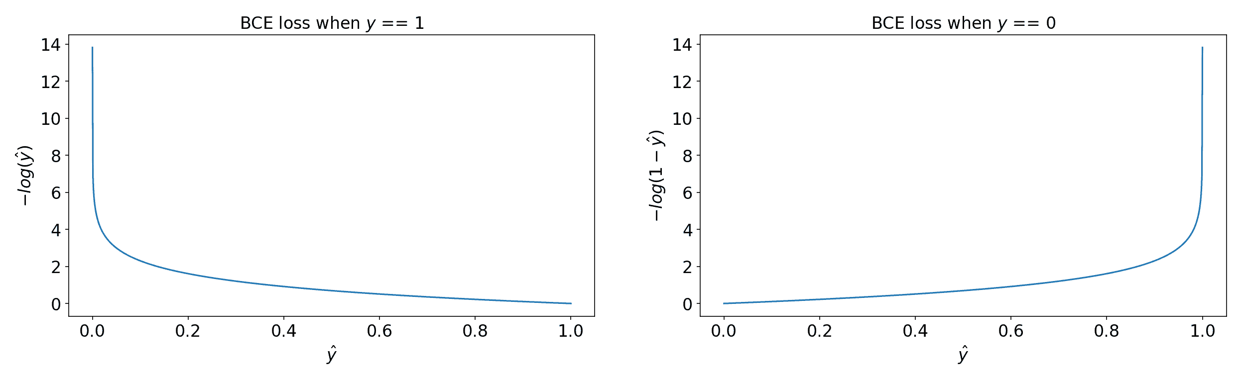
Binary Crossentropy (BCE)

Binary crossentropy is commonly used for binary classification problems. It measures the difference between the predicted probability $\overset{y}{^}$ and the true label $y$ as follows:

$L = - \frac{1}{N} i = 1 \sum N [y_{i} lo g (\overset{y}{^}_{i}) + (1 - y_{i}) lo g (1 - \overset{y}{^}_{i})]$

TensorFlow Implementation

import tensorflow as tf
loss_fn = tf.keras.losses.BinaryCrossentropy()
y_true = [1, 0, 1, 1]
y_pred = [0.9, 0.1, 0.8, 0.6]
loss = loss_fn(y_true, y_pred)
print("Binary Crossentropy Loss:", loss.numpy())

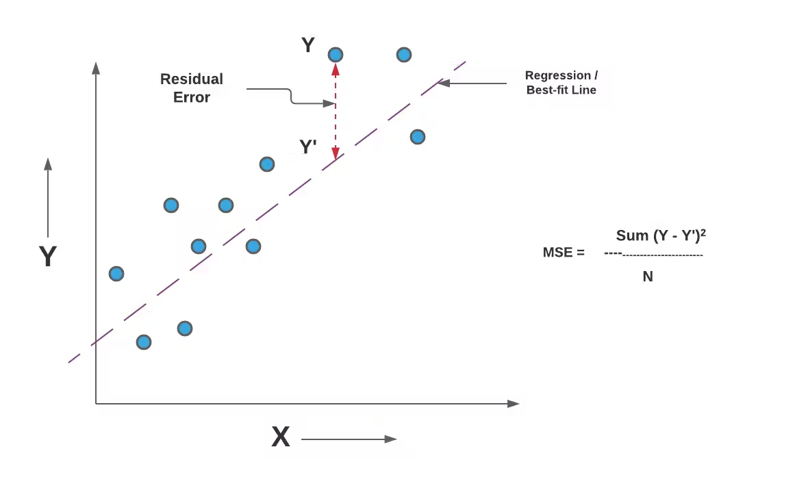
Mean Squared Error (MSE)

For regression problems, MSE calculates the average squared differences between actual and predicted values:

$L = \frac{1}{N} i = 1 \sum N (y_{i} - \overset{y}{^}_{i})^{2}$

TensorFlow Implementation

mse_fn = tf.keras.losses.MeanSquaredError()
y_true = [3.0, -0.5, 2.0, 7.0]
y_pred = [2.5, 0.0, 2.1, 7.8]
mse_loss = mse_fn(y_true, y_pred)
print("Mean Squared Error Loss:", mse_loss.numpy())

Categorical Crossentropy (CCE)

Categorical crossentropy is used for multi-class classification problems where labels are one-hot encoded. The loss function is given by:

$L = - i = 1 \sum N j = 1 \sum C y_{ij} lo g (\overset{y}{^}_{ij})$

where $C$ is the number of classes.

TensorFlow Implementation

cce_fn = tf.keras.losses.CategoricalCrossentropy()
y_true = [[0, 0, 1], [0, 1, 0]]  # One-hot encoded labels
y_pred = [[0.1, 0.2, 0.7], [0.2, 0.6, 0.2]]  # Model predictions
cce_loss = cce_fn(y_true, y_pred)
print("Categorical Crossentropy Loss:", cce_loss.numpy())

Sparse Categorical Crossentropy (SCCE)

Sparse categorical crossentropy is similar to categorical crossentropy but used when labels are not one-hot encoded (i.e., they are integers instead of vectors).

TensorFlow Implementation

scce_fn = tf.keras.losses.SparseCategoricalCrossentropy()
y_true = [2, 1]  # Integer labels
y_pred = [[0.1, 0.2, 0.7], [0.2, 0.6, 0.2]]  # Model predictions
scce_loss = scce_fn(y_true, y_pred)
print("Sparse Categorical Crossentropy Loss:", scce_loss.numpy())

Choosing the Right Loss Function

Problem Type	Suitable Loss Function	Example Application
Binary Classification	BinaryCrossentropy	Spam detection
Multi-class Classification (one-hot)	CategoricalCrossentropy	Image classification
Multi-class Classification (integer labels)	SparseCategoricalCrossentropy	Sentiment analysis
Regression	MeanSquaredError	House price prediction

Each loss function serves a different purpose and is chosen based on the nature of the problem. For classification tasks, crossentropy-based losses are preferred, while for regression, MSE is commonly used. Understanding the structure of your dataset and the expected output format is crucial when selecting the right loss function.

Training Details Main Concepts

Epochs

An epoch represents one complete pass of the entire training dataset through the neural network. During each epoch, the model updates its weights based on the error calculated from the loss function.

If we train for one epoch, the model sees each training sample exactly once.
If we train for multiple epochs, the model repeatedly sees the same data and continuously updates its weights to improve performance.

Choosing the Number of Epochs

Too Few Epochs → The model may underfit, meaning it has not learned enough patterns from the data.
Too Many Epochs → The model may overfit, meaning it memorizes the training data but generalizes poorly to new data.
The optimal number of epochs is typically determined using early stopping, which monitors validation loss and stops training when the loss starts increasing (a sign of overfitting).

TensorFlow Implementation

model.fit(X_train, y_train, epochs=50, batch_size=32, validation_data=(X_val, y_val))

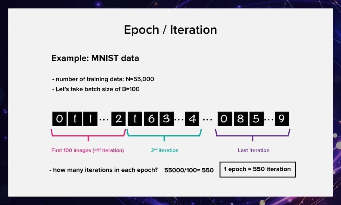
Batch Size

Instead of feeding the entire dataset into the model at once, training is performed in smaller subsets called batches.

Key Concepts:

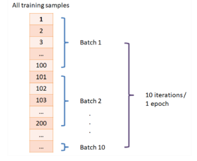
Batch Size: The number of training samples processed before updating the model's weights.
Iteration: One update of the model’s weights after processing a batch.
Steps Per Epoch: If we have N training samples and batch size B, then the number of steps per epoch is N/B.

Choosing Batch Size

Small Batch Sizes (e.g., 16, 32):
- Require less memory.
- Provide noisy but effective updates (better generalization).
Large Batch Sizes (e.g., 256, 512, 1024):
- Require more memory.
- Lead to smoother but potentially less generalized updates.

TensorFlow Implementation

model.fit(X_train, y_train, epochs=20, batch_size=64)

Validation Data

A validation set is a separate portion of the dataset that is not used for training. It helps monitor the model's performance and detect overfitting.

Differences Between Training, Validation, and Test Data:

Data Type	Purpose
Training Set	Used for updating model weights during training.
Validation Set	Used to tune hyperparameters and detect overfitting.
Test Set	Used to evaluate final model performance on unseen data.

How to Split Data:

A common split is 80% training, 10% validation, 10% test, but this can vary based on dataset size.

TensorFlow Implementation

from sklearn.model_selection import train_test_split

X_train, X_val, y_train, y_val = train_test_split(X, y, test_size=0.2, random_state=42)

model.fit(X_train, y_train, epochs=30, batch_size=32, validation_data=(X_val, y_val))

Activation Functions

1. Why Do We Need Activation Functions?

Without an activation function, a neural network with multiple layers behaves like a single-layer linear model because:

$f (x) = W x + b$

is just a linear transformation. Activation functions introduce non-linearity, allowing the network to learn complex patterns.

If we do not apply non-linearity, no matter how many layers we stack, the final output remains a linear function of the input. Activation functions solve this by enabling the model to approximate complex, non-linear relationships.

2. Common Activation Functions

Sigmoid (Logistic Function)

$σ (x) = \frac{1}{1 + e ^{- x}}$

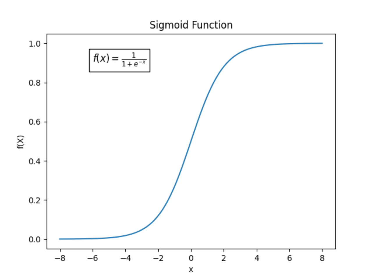
Range: (0, 1)
Used in: Binary classification problems
Pros: Outputs can be interpreted as probabilities.
Cons: Vanishing gradients for very large or very small values of ( x ), making training slow.

ReLU (Rectified Linear Unit)

$f (x) = max (0, x)$

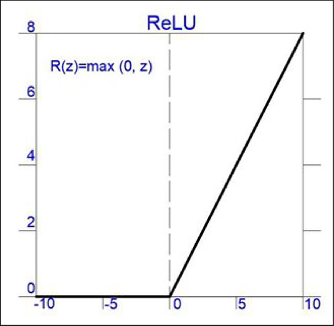
Range: [0, ∞)
Used in: Hidden layers of deep neural networks.
Pros: Helps with gradient flow and avoids vanishing gradients.
Cons: Can suffer from dying ReLU problem (where neurons output 0 and stop learning if input is negative).

Leaky ReLU

$f (x) = max (0.01 x, x)$

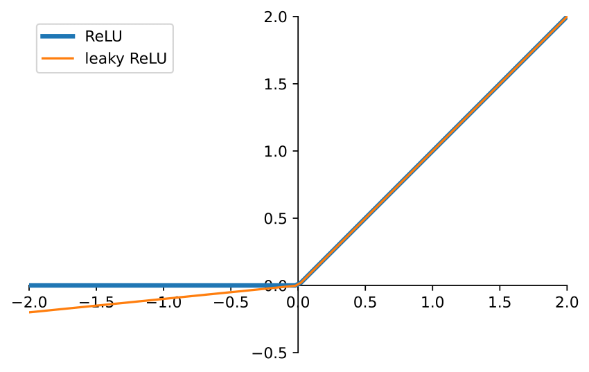
Range: (-∞, ∞)
Used in: Hidden layers as an alternative to ReLU.
Pros: Prevents the dying ReLU problem.
Cons: Small negative slope may still lead to slow learning.

Softmax

$σ (x * i) = \frac{e ^{x_{i}}}{\sum * j e ^{x_{j}}}$

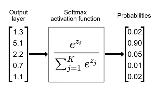
Used in: Multi-class classification (output layer).
Pros: Outputs a probability distribution (each class gets a probability between 0 and 1, summing to 1).
Cons: Can lead to numerical instability when exponentiating large numbers.

Linear Activation

$f (x) = x$

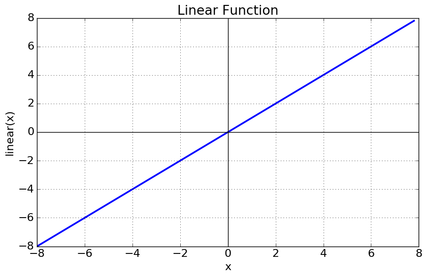
Used in: Regression problems (output layer).
Pros: No constraints on output values.
Cons: Not useful for classification since it doesn’t map values to a specific range.

3. Choosing the Right Activation Function

Layer	Recommended Activation Function	Explanation
Hidden Layers	ReLU (or Leaky ReLU if ReLU is dying)	Helps with deep networks by maintaining gradient flow
Output Layer (Binary Classification)	Sigmoid	Outputs probabilities for two-class classification
Output Layer (Multi-Class Classification)	Softmax	Converts logits into probability distributions
Output Layer (Regression)	Linear	Directly outputs numerical values

Softmax vs. Sigmoid: Key Differences

Sigmoid is mainly used for binary classification, mapping values to (0,1), which can be interpreted as class probabilities.
Softmax is used for multi-class classification, producing a probability distribution over multiple classes.

If you use sigmoid for multi-class problems, each output node will act independently, making it difficult to ensure they sum to 1. Softmax ensures that outputs sum to 1, providing a clearer probabilistic interpretation.

Improved Implementation of Softmax

Why Use Linear Instead of Softmax in the Output Layer?

When implementing a neural network for classification, we often pass logits (raw outputs) directly into the loss function instead of applying softmax explicitly.

Mathematically, if we apply softmax explicitly:

$L = - \sum y_{i} lo g (σ (z_{i}))$

where ( \sigma(z) ) is the softmax function.

However, if we pass raw logits (without softmax) into the cross-entropy loss function, TensorFlow applies the log-softmax trick internally:

$L = - \sum y_{i} z_{i} + lo g \sum e^{z_{i}}$

This avoids computing large exponentials, improving numerical stability and reducing computation cost.

TensorFlow Implementation

Instead of:

model = tf.keras.Sequential([
    tf.keras.layers.Dense(128, activation='relu'),
    tf.keras.layers.Dense(64, activation='relu'),
    tf.keras.layers.Dense(10, activation='softmax')  # Explicit softmax
])
model.compile(loss=tf.keras.losses.SparseCategoricalCrossentropy(), optimizer='adam')

Use:

model = tf.keras.Sequential([
    tf.keras.layers.Dense(128, activation='relu'),
    tf.keras.layers.Dense(64, activation='relu'),
    tf.keras.layers.Dense(10)  # No activation here!
])
model.compile(loss=tf.keras.losses.SparseCategoricalCrossentropy(from_logits=True), optimizer='adam')

This allows TensorFlow to handle softmax internally, avoiding unnecessary computation and improving numerical precision.