Optimizers and Layer Types
- Optimizers in Deep Learning
- Choosing the Right Optimizer
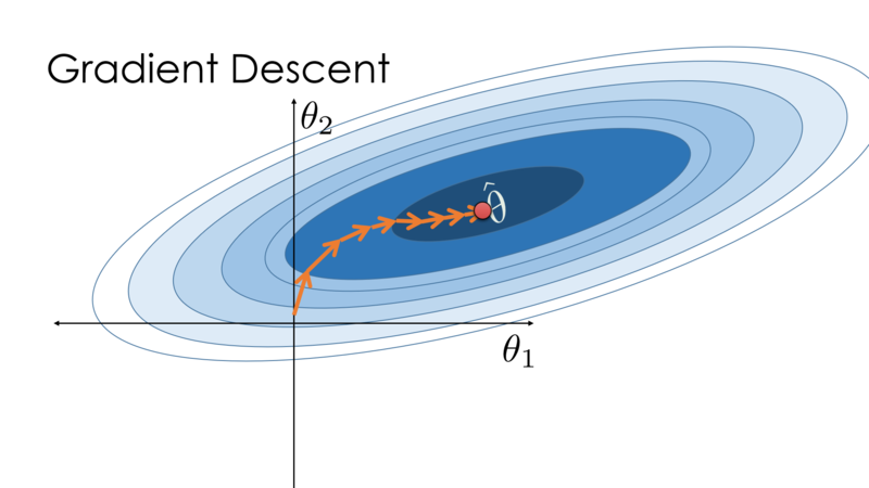
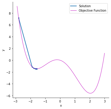
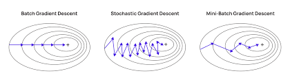
- Gradient Descent (GD)
- Stochastic Gradient Descent (SGD)
- Stochastic Gradient Descent with Momentum (SGD-Momentum)
- Mini-Batch Gradient Descent
- Adagrad (Adaptive Gradient Descent)
- RMSprop (Root Mean Square Propagation)
- AdaDelta
- Adam (Adaptive Moment Estimation)
- Hands-on Optimizers
- Table Analysis
- Conclusion
- Additional Layer Types in Neural Networks
Optimizers in Deep Learning
Optimizers play a crucial role in training deep learning models by adjusting the model parameters to minimize the loss function. Different optimization algorithms have been developed to improve convergence speed, accuracy, and stability. In this article, we explore various optimizers used in deep learning, their mathematical formulations, and practical implementations.
Choosing the Right Optimizer
Choosing the right optimizer depends on several factors, including:
- The nature of the dataset
- The complexity of the model
- The presence of noisy gradients
- The required computational efficiency
Below, we examine different types of optimizers along with their mathematical formulations.
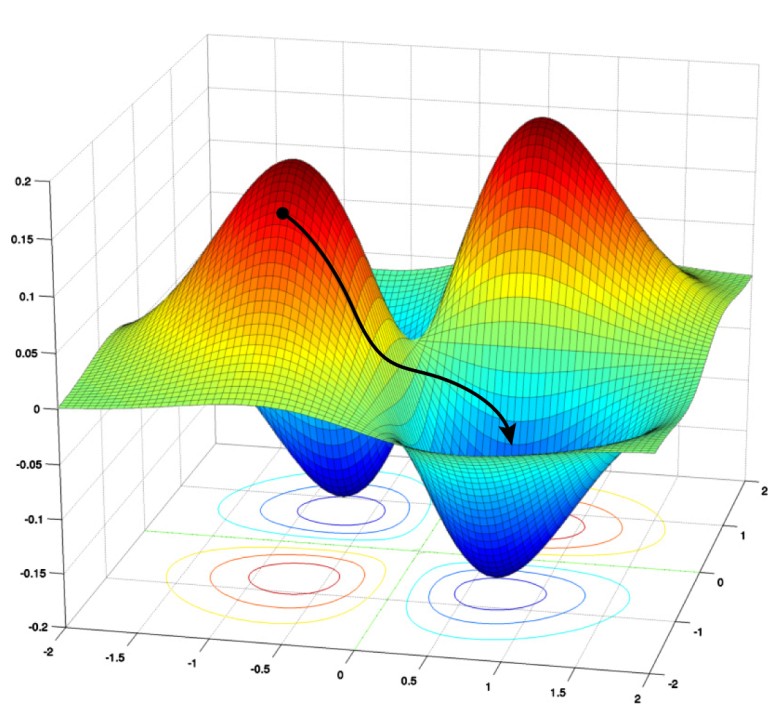
Gradient Descent (GD)
Mathematical Formulation
Gradient Descent updates model parameters iteratively using the gradient of the loss function :
where:
- is the learning rate
- is the gradient of the loss function
Characteristics
- Computes gradient over the entire dataset
- Slow for large datasets
- Prone to getting stuck in local minima
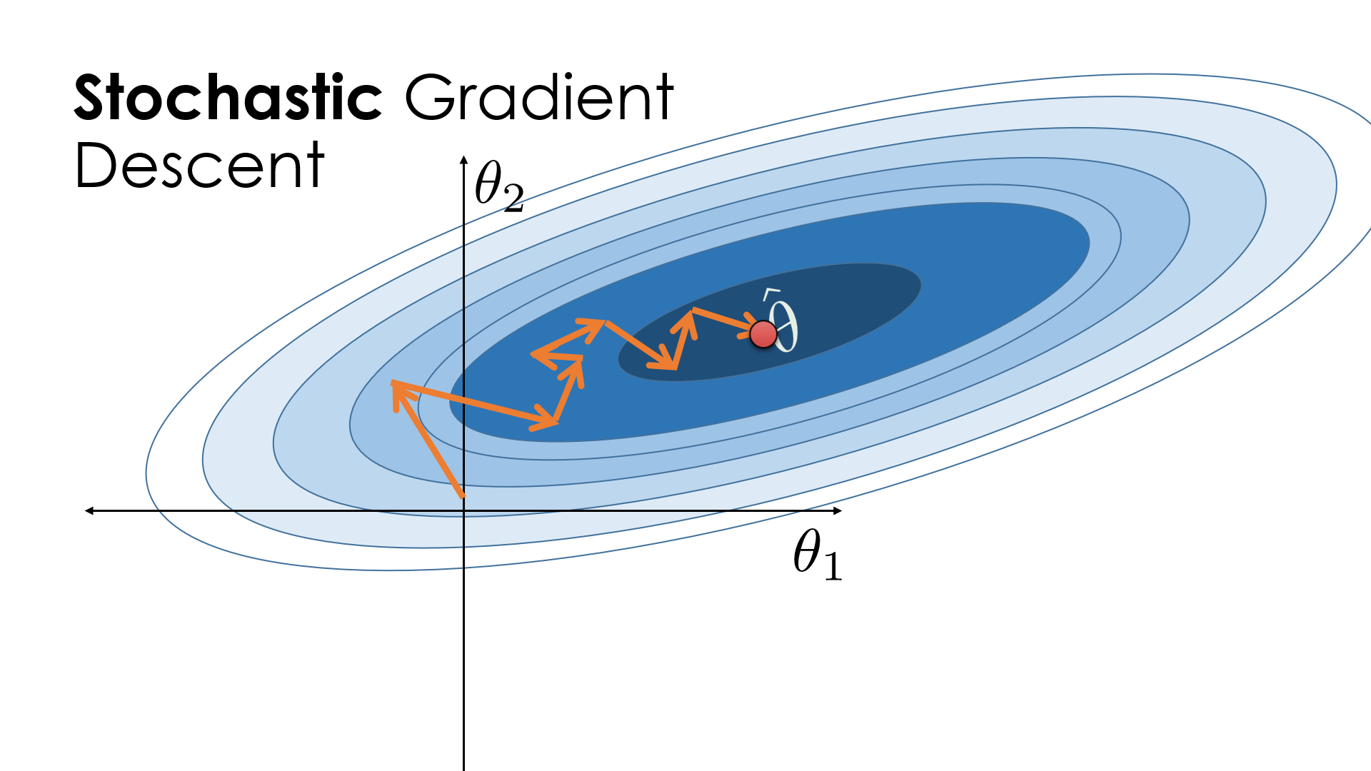
Stochastic Gradient Descent (SGD)
Gradient descent struggles with massive datasets, making stochastic gradient descent (SGD) a better alternative. Unlike standard gradient descent, SGD updates model parameters using small, randomly selected data batches, improving computational efficiency.
SGD initializes parameters and learning rate , then shuffles data at each iteration, updating based on mini-batches. This introduces noise, requiring more iterations to converge, but still reduces overall computation time compared to full-batch gradient descent.
For large datasets where speed matters, SGD is preferred over batch gradient descent.
Mathematical Formulation
Instead of computing the gradient over the entire dataset, SGD updates using a single data point:
where is a single training example.
Characteristics
- Faster than full-batch gradient descent
- High variance in updates
- Introduces noise, which can help escape local minima
Stochastic Gradient Descent with Momentum (SGD-Momentum)
SGD follows a noisy optimization path, requiring more iterations and longer computation time. To speed up convergence, SGD with momentum is used.
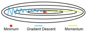
Momentum helps stabilize updates by adding a fraction of the previous update to the current one, reducing oscillations and accelerating convergence. However, a high momentum term requires lowering the learning rate to avoid overshooting the optimal minimum.
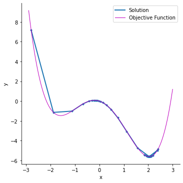
While momentum improves speed, too much momentum can cause instability and poor accuracy. Proper tuning is essential for effective optimization.
Mathematical Formulation
Momentum helps accelerate SGD by maintaining a velocity term:
where:
- is the momentum term
- is a momentum coefficient (typically 0.9)
Characteristics
- Reduces oscillations
- Faster convergence
Mini-Batch Gradient Descent
Mini-batch gradient descent optimizes training by using a subset of data instead of the entire dataset, reducing the number of iterations needed. This makes it faster than both stochastic and batch gradient descent while being more efficient and memory-friendly.
Key Advantages
- Balances speed and accuracy by reducing noise compared to SGD but keeping updates more dynamic than batch gradient descent.
- Doesn’t require loading all data into memory, improving implementation efficiency.
Limitations
- Requires tuning the mini-batch size (typically 32) for optimal accuracy.
- May lead to poor final accuracy in some cases, requiring alternative approaches.
Mathematical Formulation
Instead of updating with the entire dataset or a single example, mini-batch GD uses a small batch of samples:
Adagrad (Adaptive Gradient Descent)
Adagrad differs from other gradient descent algorithms by using a unique learning rate for each iteration, adjusting based on parameter changes. Larger parameter updates lead to smaller learning rate adjustments, making it effective for datasets with both sparse and dense features.
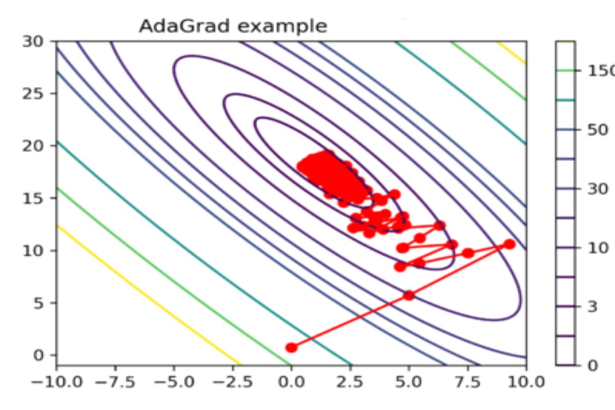
Key Advantages
- Eliminates manual learning rate tuning by adapting automatically.
- Faster convergence compared to standard gradient descent methods.
Limitations
- Aggressively reduces the learning rate over time, which can slow learning and harm accuracy.
- The accumulation of squared gradients in the denominator causes the learning rate to become too small, limiting further model improvements.
Mathematical Formulation
Adagrad adapts learning rates for each parameter:
where accumulates past squared gradients:
Characteristics
- Suitable for sparse data
- Learning rate decreases over time
RMSprop (Root Mean Square Propagation)
RMSProp improves stability by adapting step sizes per weight, preventing large gradient fluctuations. It maintains a moving average of squared gradients to adjust learning rates dynamically.
Mathematical Formulation
Pros
- Faster convergence with smoother updates.
- Less tuning than other gradient descent variants.
- More stable than Adagrad by preventing extreme learning rate decay.
Cons
- Requires manual learning rate tuning, and default values may not always be optimal.
AdaDelta
Mathematical Formulation
AdaDelta modifies Adagrad by using an exponentially decaying average of past squared gradients:
where is the moving average.
Characteristics
- Addresses diminishing learning rates in Adagrad
- No need to manually set a learning rate
Adam (Adaptive Moment Estimation)
Adam (Adaptive Moment Estimation) is a widely used deep learning optimizer that extends SGD by dynamically adjusting learning rates for each weight. It combines AdaGrad and RMSProp to balance adaptive learning rates and stable updates.
Mathematical Formulation
Adam combines momentum and RMSprop:
where and are bias-corrected estimates.
Key Features
- Uses first (mean) and second (variance) moments of gradients.
- Faster convergence with minimal tuning.
- Low memory usage and efficient computation.
Downsides
- Prioritizes speed over generalization, making SGD better for some cases.
- May not always be ideal for every dataset.
Adam is the default choice for many deep learning tasks but should be selected based on the dataset and training requirements.
Hands-on Optimizers
Import Necessary Libraries
import keras
from keras.datasets import mnist
from keras.models import Sequential
from keras.layers import Dense, Dropout, Flatten
from keras.layers import Conv2D, MaxPooling2D
from keras import backend as K
(x_train, y_train), (x_test, y_test) = mnist.load_data()
print(x_train.shape, y_train.shape)
Load the Dataset
x_train= x_train.reshape(x_train.shape[0],28,28,1)
x_test=  x_test.reshape(x_test.shape[0],28,28,1)
input_shape=(28,28,1)
y_train=keras.utils.to_categorical(y_train)#,num_classes=)
y_test=keras.utils.to_categorical(y_test)#, num_classes)
x_train= x_train.astype('float32')
x_test= x_test.astype('float32')
x_train /= 255
x_test /=255
Build the Model
batch_size=64

num_classes=10

epochs=10

def build_model(optimizer):

    model=Sequential()

    model.add(Conv2D(32,kernel_size=(3,3),activation='relu',input_shape=input_shape))

    model.add(MaxPooling2D(pool_size=(2,2)))

    model.add(Dropout(0.25))

    model.add(Flatten())

    model.add(Dense(256, activation='relu'))

    model.add(Dropout(0.5))

    model.add(Dense(num_classes, activation='softmax'))

    model.compile(loss=keras.losses.categorical_crossentropy, optimizer= optimizer, metrics=['accuracy'])

    return model
Train the Model
optimizers = ['Adadelta', 'Adagrad', 'Adam', 'RMSprop', 'SGD']

for i in optimizers:

model = build_model(i)

hist=model.fit(x_train, y_train, batch_size=batch_size, epochs=epochs, verbose=1, validation_data=(x_test,y_test))
Table Analysis
| Optimizer | Epoch 1 (Val Acc | Val Loss) | Epoch 5 (Val Acc | Val Loss) | Epoch 10 (Val Acc | Val Loss) | Total Time |
|---|---|---|---|---|---|---|---|
| Adadelta | .4612 | 2.2474 | .7776 | 1.6943 | .8375 | 0.9026 | 8:02 min |
| Adagrad | .8411 | .7804 | .9133 | .3194 | .9286 | 0.2519 | 7:33 min |
| Adam | .9772 | .0701 | .9884 | .0344 | .9908 | .0297 | 7:20 min |
| RMSprop | .9783 | .0712 | .9846 | .0484 | .9857 | .0501 | 10:01 min |
| SGD with momentum | .9168 | .2929 | .9585 | .1421 | .9697 | .1008 | 7:04 min |
| SGD | .9124 | .3157 | .9569 | 1.451 | .9693 | .1040 | 6:42 min |
The above table shows the validation accuracy and loss at different epochs. It also contains the total time that the model took to run on 10 epochs for each optimizer. From the above table, we can make the following analysis.
- The adam optimizer shows the best accuracy in a satisfactory amount of time.
- RMSprop shows similar accuracy to that of Adam but with a comparatively much larger computation time.
- Surprisingly, the SGD algorithm took the least time to train and produced good results as well. But to reach the accuracy of the Adam optimizer, SGD will require more iterations, and hence the computation time will increase.
- SGD with momentum shows similar accuracy to SGD with unexpectedly larger computation time. This means the value of momentum taken needs to be optimized.
- Adadelta shows poor results both with accuracy and computation time.
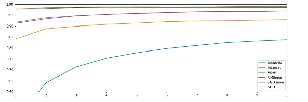
You can analyze the accuracy of each optimizer with each epoch from the above graph.
Conclusion
Different optimizers offer unique advantages based on the dataset and model architecture. While SGD is the simplest, Adam is often preferred for deep learning tasks due to its adaptive learning rate and momentum.
By understanding these optimizers, you can fine-tune deep learning models for optimal performance!
Additional Layer Types in Neural Networks
In deep learning, different layer types serve distinct purposes, helping neural networks learn complex representations. This section explores various layer types, their mathematical foundations, and practical implementations.
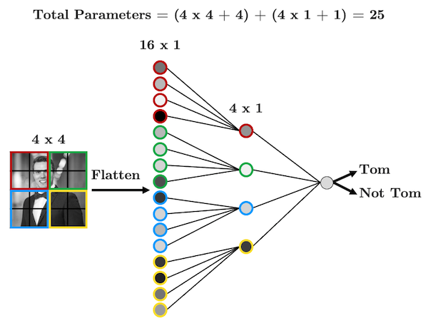
Dense Layer (Fully Connected Layer)
A Dense layer is a fundamental layer where each neuron is connected to every neuron in the previous layer.
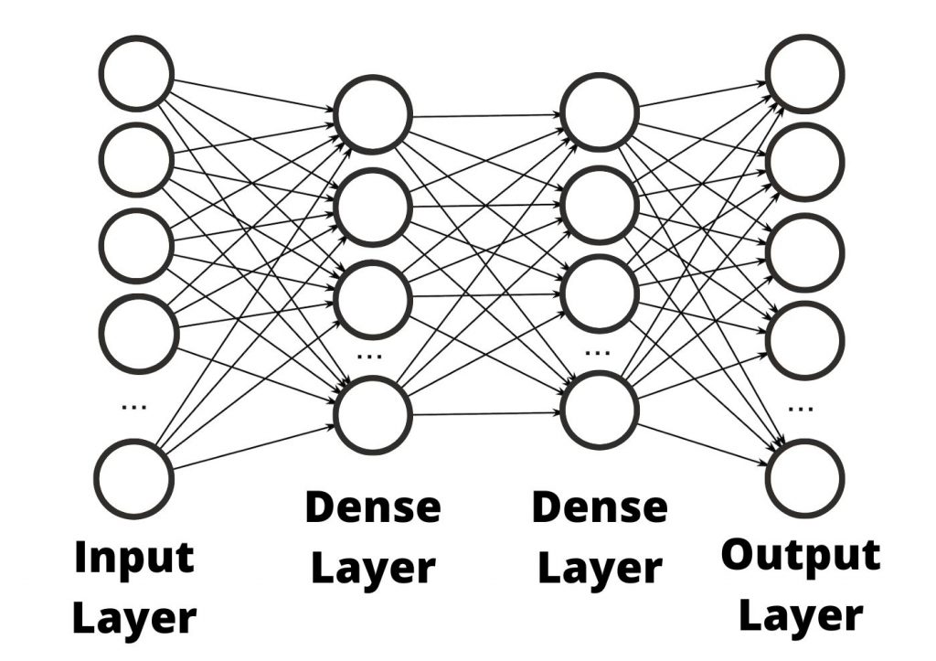
Mathematical Representation:
Given an input vector of size , weights of size , and bias of size , the output is calculated as:
where is an activation function such as ReLU, Sigmoid, or Softmax.
Implementation in TensorFlow:
import tensorflow as tf
from tensorflow.keras.models import Sequential
from tensorflow.keras.layers import Dense

model = Sequential([
    Dense(64, activation='relu', input_shape=(100,)),
    Dense(32, activation='relu'),
    Dense(10, activation='softmax')
])
model.summary()
Convolutional Layer (Conv2D)
A Convolutional layer is used in image processing, applying filters (kernels) to extract features from input images.
Mathematical Representation:
For an input image and a filter , the convolution operation is defined as:
Implementation in TensorFlow:
from tensorflow.keras.layers import Conv2D

model = Sequential([
    Conv2D(32, kernel_size=(3,3), activation='relu', input_shape=(28,28,1)),
    Conv2D(64, kernel_size=(3,3), activation='relu'),
])
model.summary()
Pooling Layer (MaxPooling & AveragePooling)
Pooling layers reduce dimensionality while preserving important features.
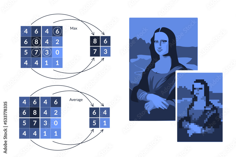
Max Pooling:
Average Pooling:
Implementation:
from tensorflow.keras.layers import MaxPooling2D, AveragePooling2D

model = Sequential([
    MaxPooling2D(pool_size=(2,2)),
    AveragePooling2D(pool_size=(2,2))
])
model.summary()
Recurrent Layer (RNN, LSTM, GRU)
Recurrent layers process sequential data by maintaining memory of past inputs.
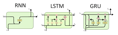
RNN Mathematical Model:
LSTM Update Equations:
Implementation:
from tensorflow.keras.layers import SimpleRNN, LSTM, GRU

model = Sequential([
    LSTM(64, return_sequences=True, input_shape=(100, 10)),
    GRU(32)
])
model.summary()
Dropout Layer
The Dropout layer randomly sets a fraction of input units to 0 to prevent overfitting.
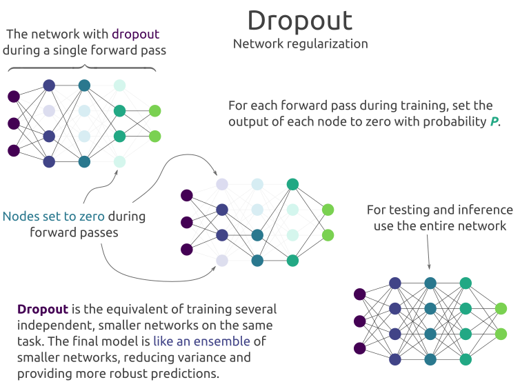
Mathematical Explanation:
During training, for each neuron, the probability of being kept is :
Implementation:
from tensorflow.keras.layers import Dropout

model = Sequential([
    Dense(128, activation='relu'),
    Dropout(0.5),
    Dense(64, activation='relu'),
    Dropout(0.3),
    Dense(10, activation='softmax')
])
model.summary()
Comparison Table
| Layer Type | Purpose | Typical Use Case |
|---|---|---|
| Dense | Fully connected layer | General deep learning models |
| Conv2D | Feature extraction | Image processing |
| Pooling | Downsampling | CNNs to reduce size |
| RNN | Sequential processing | Time-series, NLP |
| LSTM/GRU | Long-term memory retention | Language models |
| Dropout | Overfitting prevention | Regularization in deep networks |
Conclusion
Understanding different types of layers is crucial in designing effective deep learning models. Choosing the right layers based on the data type and problem domain significantly impacts model performance. Experimenting with combinations of these layers is key to optimizing results.