Model Evaluation, Selection, and Improvement
- Evaluating a Model
- Model Selection and Training/Validation/Test Sets
- Diagnosing Bias and Variance
- Regularization and Bias-Variance Tradeoff
- Establishing a Baseline Level of Performance
- Iterative Loop of ML Development
- Adding Data: Data Augmentation & Synthesis
- Transfer Learning: Using Data from a Different Task
- Error Metrics for Skewed Datasets
Evaluating a Model
A metric is a numerical measure used to assess the performance of a model on a given dataset. Metrics help quantify how well a model is making predictions and whether it meets the desired objectives. The choice of metric depends on the nature of the problem:
- For classification tasks, we often measure how accurately a model assigns labels.
- For regression tasks, we evaluate how close the model’s predictions are to actual values.
- In other domains like natural language processing (NLP) or computer vision, specialized metrics are used.
However, a high metric value does not always mean a model is truly effective. For example:
- In an imbalanced dataset, accuracy might be misleading. A model predicting the majority class 100% of the time can have high accuracy but perform poorly overall.
- A regression model with a low mean squared error (MSE) might still fail in real-world applications if it makes large errors in critical cases.
Key Metrics for Model Evaluation
Classification Metrics
- Accuracy: Measures the percentage of correctly predicted instances.
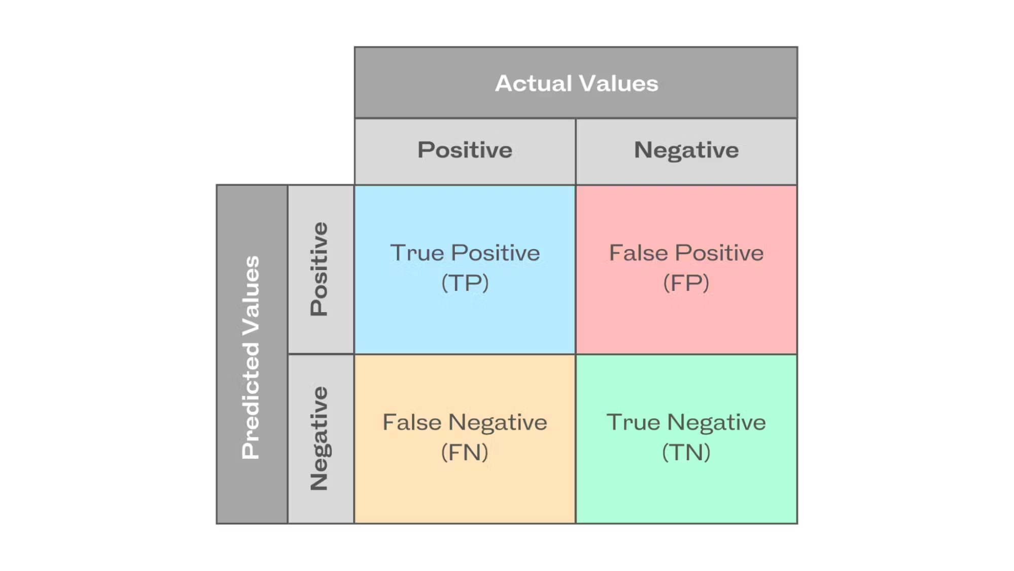
- Precision: The fraction of true positive predictions among all positive predictions.
- Recall: The fraction of actual positives correctly identified.
- F1-score: The harmonic mean of precision and recall, useful for imbalanced datasets.
- ROC-AUC (Receiver Operating Characteristic - Area Under Curve): Evaluates the model’s ability to distinguish between classes.
Regression Metrics
- Mean Squared Error (MSE): Measures the average squared difference between predicted and actual values.
- Mean Absolute Error (MAE): Measures the average absolute difference.
- R-squared (R²): Indicates how well the model explains variance in the data.
Other Metrics
- Log loss: Used for probabilistic classification models.
- BLEU score: Measures similarity in NLP tasks.
- Intersection over Union (IoU): Used in object detection to measure overlap between predicted and actual bounding boxes.
Choosing the Right Metric
Suppose we are building a spam classifier. If 99% of emails are non-spam, a naive model predicting “not spam” for all emails will have 99% accuracy but be completely useless. In this case, precision and recall are more meaningful metrics because they tell us how well the model detects actual spam emails without too many false positives.
Thus, choosing the right metric is just as important as achieving a high score. A well-performing model is one that aligns with the real-world objective of the task.
Model Selection and Training/Validation/Test Sets
Selecting the right model is essential for achieving high performance on unseen data. A model that performs well on training data but poorly on new data is overfitting, while a model that is too simple may underfit. To properly evaluate a model and fine-tune its performance, we split the dataset into three key subsets:
Training Set
The training set is the portion of the data used to train the machine learning model. The model learns patterns from this data by adjusting its internal parameters. However, evaluating the model only on the training set is misleading because the model might memorize the data instead of generalizing from it.
Validation Set
The validation set is a separate portion of the dataset that is used to tune hyperparameters and select the best model architecture. Hyperparameters are external configuration settings that are not learned by the model but instead set manually or through automated search methods. Examples of hyperparameters include:
- Learning rate
- Number of hidden layers in a neural network
- Regularization parameters (L1, L2)
- Batch size
By testing different hyperparameter values on the validation set, we can find the combination that leads to the best generalization performance. However, if the validation set is too small or used excessively for tuning, the model might start overfitting to it.
Test Set
The test set is used only once, after model training and hyperparameter tuning, to evaluate the final model’s performance. The test set should remain completely unseen during training and validation to provide an unbiased estimate of how the model will perform on real-world data.
Cross-Validation
Cross-validation is a technique to make better use of available data and improve model selection. Instead of relying on a single validation set, we divide the dataset into multiple subsets and perform training and validation multiple times. The most common approach is k-fold cross-validation, which works as follows:
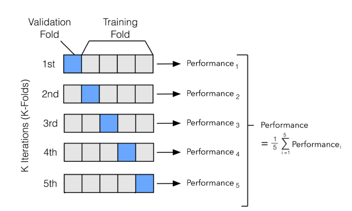
- The dataset is divided into k equal-sized folds.
- The model is trained on k-1 folds and validated on the remaining one.
- This process is repeated k times, with each fold serving as the validation set once.
- The final performance metric is the average of all validation scores.
For example, in 5-fold cross-validation, the dataset is split into 5 parts. The model is trained on 4 parts and validated on the remaining one, and this process repeats until each part has been used as a validation set once. This reduces the risk of selecting a model that performs well on just one specific validation set but poorly on unseen data.
Cross-validation is especially useful when working with small datasets since it allows more efficient use of data. However, it can be computationally expensive, especially for deep learning models, where training is time-consuming.
By using training, validation, and test sets appropriately—along with cross-validation where necessary—we can make informed decisions about model selection and ensure good generalization to new data.
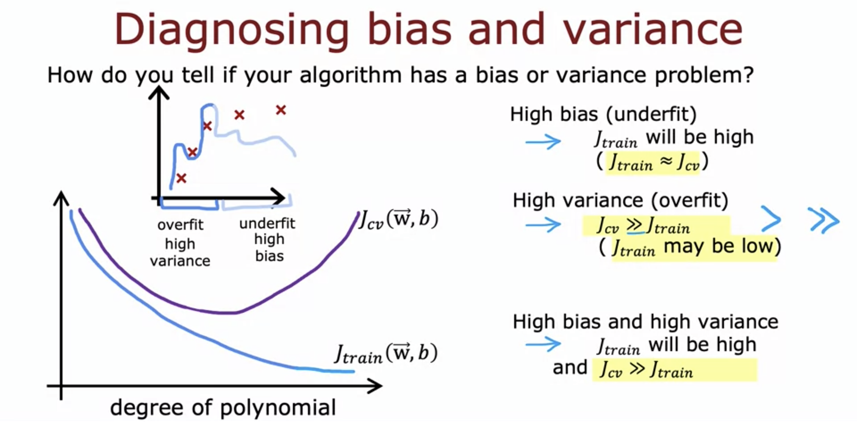
Diagnosing Bias and Variance
Bias and variance are two key factors that determine a model’s ability to generalize to unseen data. To understand these concepts, let’s analyze the simple linear model:
A well-performing model should generalize well, meaning it captures the essential patterns in the data without memorizing noise. Let’s break this down using the equation.
| Issue | Description | Effects | Impact of More Data |
|---|---|---|---|
| High Bias (Underfitting) | Model is too simple and cannot capture underlying patterns. | - Poor performance on both training and test sets. - Model is too simplistic. | Increasing training data does not improve performance. |
| High Variance (Overfitting) | Model is too complex and memorizes training data, including noise. | - Training error is very low, but test error is high. - Model learns noise instead of actual patterns. | Increasing training data can help generalization. |
Regularization and Bias-Variance Tradeoff
To prevent overfitting, we introduce regularization, which penalizes large weights.
The regularized loss function:
where:
- is the original loss function (e.g., Mean Squared Error),
- is the regularization strength,
- is the penalty term (L1 or L2).
Effect of Regularization
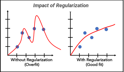
- If is too low, the model can overfit ( values become large).
- If is too high, the model becomes too simple ( values shrink too much).
- The ideal value balances bias and variance.
Establishing a Baseline Level of Performance
A baseline model helps measure improvement. Common baselines include:
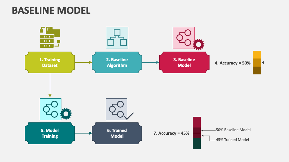
- Random classifiers (for classification tasks)
- Mean predictions (for regression tasks)
- Simple heuristic-based methods
A model must outperform the baseline to be considered useful.
Iterative Loop of ML Development
Machine learning development follows an iterative cycle:
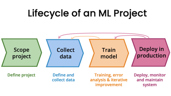
- Train a baseline model.
- Diagnose bias/variance errors.
- Adjust model complexity, regularization, or data strategy.
- Repeat until performance is satisfactory.
Adding Data: Data Augmentation & Synthesis
One of the most effective ways to improve a model’s generalization ability is by increasing the amount of training data. More data helps the model learn patterns that are not specific to the training set, reducing overfitting and improving robustness.
Data Augmentation
Data Augmentation refers to artificially increasing the size of the training dataset by applying transformations to existing data. It is particularly useful in fields like computer vision and NLP, where collecting labeled data is expensive and time-consuming.
Common Data Augmentation Techniques
-
Image Data Augmentation (Used in deep learning for computer vision tasks):
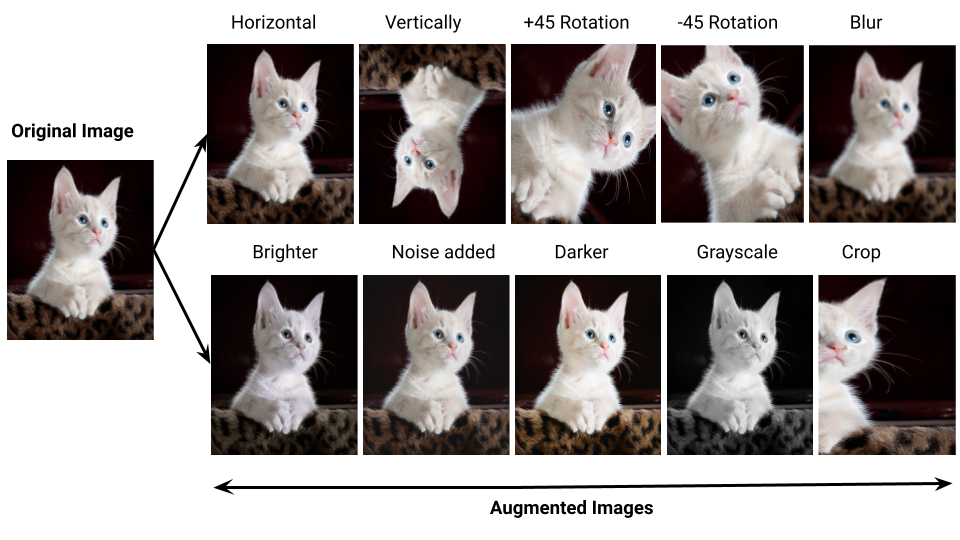
- Rotation: Rotating images by small degrees to simulate different perspectives.
- Cropping: Randomly cropping parts of the image to focus on different areas.
- Flipping: Horizontally or vertically flipping images.
- Scaling: Resizing images while maintaining aspect ratios.
- Brightness/Contrast Adjustments: Modifying brightness and contrast to simulate lighting variations.
- Noise Injection: Adding Gaussian noise to simulate different sensor conditions.
Example in TensorFlow/Keras:
from tensorflow.keras.preprocessing.image import ImageDataGenerator datagen = ImageDataGenerator( rotation_range=20, width_shift_range=0.1, height_shift_range=0.1, horizontal_flip=True, brightness_range=[0.8, 1.2] ) augmented_images = datagen.flow(x_train, y_train, batch_size=32) -
Text Data Augmentation (Used in NLP models):
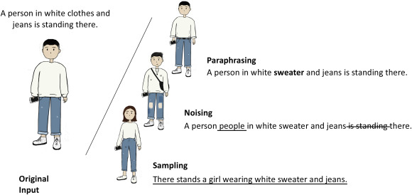
-
Synonym Replacement: Replacing words with their synonyms.
-
Random Insertion: Adding random words from the vocabulary.
-
Back Translation: Translating text to another language and back to introduce variation.
-
Sentence Shuffling: Reordering words or sentences slightly.
Example using
nlpaug:
import nlpaug.augmenter.word as naw aug = naw.SynonymAug(aug_src='wordnet') text = "Deep learning models require large amounts of data." augmented_text = aug.augment(text) print(augmented_text) -
-
Time-Series Data Augmentation (Used in financial data, speech processing):
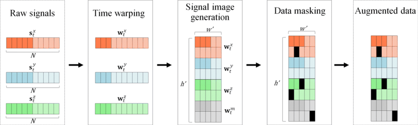
- Time Warping: Stretching or compressing time series data.
- Jittering: Adding small random noise to numerical values.
- Scaling: Multiplying data points by a random factor.
Data Synthesis
Data Synthesis involves generating entirely new data points that mimic real-world distributions. This is useful when real data is scarce or difficult to obtain.
Common Data Synthesis Techniques
-
Generative Adversarial Networks (GANs)
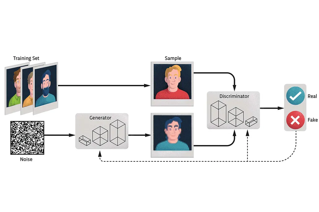
- GANs can generate realistic-looking images, text, or audio by learning the underlying distribution of the dataset.
- Example: GAN-generated human faces (thispersondoesnotexist.com).
Example GAN code using PyTorch:
import torch.nn as nn import torch.optim as optim class Generator(nn.Module): def __init__(self): super(Generator, self).__init__() self.fc = nn.Linear(100, 784) # 100-d noise vector to 28x28 image def forward(self, x): return torch.tanh(self.fc(x)) generator = Generator() noise = torch.randn(1, 100) fake_image = generator(noise) -
Bootstrapping
- A statistical method that resamples data with replacement to create new samples.
- Useful in small datasets to increase training size.
- Often used in ensemble learning (e.g., bagging).
-
Synthetic Minority Over-sampling (SMOTE)
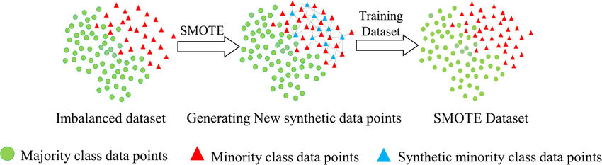
- Used in imbalanced datasets to generate synthetic minority class examples.
- Creates interpolated samples between existing data points.
- Example using
imbalanced-learn:
from imblearn.over_sampling import SMOTE from sklearn.model_selection import train_test_split X_resampled, y_resampled = SMOTE().fit_resample(X_train, y_train) -
Simulation-Based Synthesis
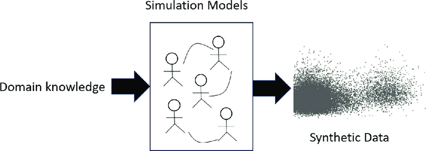
- Used in robotics, healthcare, and autonomous driving where real-world data collection is expensive or dangerous.
- Example: Self-driving cars trained on simulated environments before real-world deployment.
When to Use Data Augmentation vs. Data Synthesis?
| Method | Best for | Common Use Cases |
|---|---|---|
| Data Augmentation | Expanding existing datasets | Image classification, speech recognition |
| Data Synthesis | Creating new synthetic samples | GANs for image generation, NLP text synthesis |
Transfer Learning: Using Data from a Different Task
Transfer learning leverages pre-trained models:
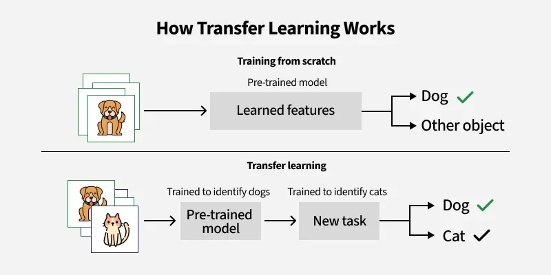
- Feature extraction: Use pre-trained model layers as feature extractors.
- Fine-tuning: Unfreeze layers and retrain on a new dataset.
Example: Using ImageNet-trained models for medical image classification.
Error Metrics for Skewed Datasets
In imbalanced datasets, accuracy alone is often misleading. For example, if a dataset has 95% negative samples and 5% positive samples, a model that always predicts “negative” will have 95% accuracy but is completely useless. Instead, we use more informative metrics:
Precision, Recall, and F1-Score
-
Precision (): Measures how many of the predicted positives are actually correct.
- High Precision: The model makes fewer false positive errors.
- Example: In an email spam filter, high precision means fewer legitimate emails are mistakenly classified as spam.
-
Recall (): Measures how many actual positives were correctly identified.
- High Recall: The model captures most of the actual positive cases.
- Example: In a medical test for cancer, high recall ensures that nearly all cancer cases are detected.
-
F1-Score: The harmonic mean of precision and recall, balancing both aspects.
- Used when both false positives and false negatives need to be minimized.
- F1-score ranges from 0 to 1, where 1 is the best possible score, indicating a perfect balance between precision and recall. However, what qualifies as a “good” or “bad” F1-score depends on the context of the problem.