Decision Trees
- Decision Tree Model
- Measuring Purity
- Choosing a Split: Information Gain
- Decision Trees for Continuous Features
- Regression Trees
- Using Multiple Decision Trees
Decision Tree Model
What is a Decision Tree?
A decision tree is a supervised machine learning algorithm used for classification and regression tasks. It mimics human decision-making by splitting data into branches based on feature values, forming a tree-like structure. The key components of a decision tree include:
- Root Node: The initial decision point that represents the entire dataset.
- Internal Nodes: Decision points where data is split based on a feature.
- Branches: The possible outcomes of a decision node.
- Leaf Nodes: The terminal nodes that provide the final classification or prediction.
graph TD;
    Root[Root Node] -->|Feature 1| Node1[Node 1];
    Root -->|Feature 2| Node2[Node 2];
    Node1 --> Leaf1[Leaf Node 1];
    Node1 --> Leaf2[Leaf Node 2];
    Node2 --> Leaf3[Leaf Node 3];
    Node2 --> Leaf4[Leaf Node 4];
Decision trees work by recursively splitting data based on a selected feature until a stopping condition is met.
Advantages and Disadvantages of Decision Trees
Advantages:
- Easy to Interpret: Decision trees provide an intuitive representation of decision-making.
- Handles Both Numerical and Categorical Data: They can work with mixed data types.
- No Need for Feature Scaling: Unlike algorithms like logistic regression or SVMs, decision trees do not require feature normalization.
- Works Well with Small Datasets: Decision trees can be effective even with limited data.
Disadvantages:
- Overfitting: Decision trees tend to learn patterns too specifically to the training data, leading to poor generalization.
- Sensitive to Noisy Data: Small variations in data can lead to different tree structures.
- Computational Complexity: For large datasets, training a deep tree can be time-consuming and memory-intensive.
Example: Classifying Fruits Using a Decision Tree
Consider a dataset containing different types of fruits characterized by their color, size, and texture. Our goal is to classify whether a given fruit is an apple or an orange.
| Color | Size | Texture | Fruit |
|---|---|---|---|
| Red | Small | Smooth | Apple |
| Green | Small | Smooth | Apple |
| Yellow | Large | Rough | Orange |
| Orange | Large | Rough | Orange |
Decision Tree Representation:
graph TD;
    Root[Is Size Large?]
    Root -- Yes --> Node1[Is Texture Rough?]
    Root -- No --> Apple[Apple]
    Node1 -- Yes --> Orange[Orange]
    Node1 -- No --> Apple[Apple]
The decision tree follows a top-down approach:
- The root node first checks whether the fruit is large.
- If yes, it checks whether the texture is rough.
- If the texture is rough, it classifies the fruit as an orange; otherwise, it’s an apple.
This example demonstrates how decision trees break down complex decision-making processes into simple binary decisions.
The learning process involves recursively splitting the dataset into smaller subsets. The splitting criterion is chosen based on purity measures such as Gini impurity or entropy. Each split creates child nodes until the stopping condition is met.
Stopping Criteria and Overfitting
A decision tree can continue growing until each leaf contains only one class. However, this often leads to overfitting, where the model memorizes the training data but fails to generalize to new data. To prevent this, stopping criteria such as:
- A minimum number of samples per leaf
- A maximum tree depth
- A minimum purity gain
can be used. Additionally, pruning techniques help reduce overfitting by removing branches that add little predictive value.
Pruning Example
- Pre-pruning: Stop the tree from growing beyond a certain depth.
- Post-pruning: Grow the full tree and then remove unimportant branches based on validation performance.
Measuring Purity
In decision trees, “purity” refers to how homogeneous the data in a given node is. A node is considered pure if it contains only samples from a single class. Measuring purity is essential for determining the best way to split a dataset to build an effective decision tree. The two most common metrics used for measuring purity are Entropy and Gini Impurity.
Entropy
Entropy, derived from information theory, measures the randomness or disorder in a dataset. The entropy equation for a binary classification problem is:
where:
- and are the proportions of each class in the set .
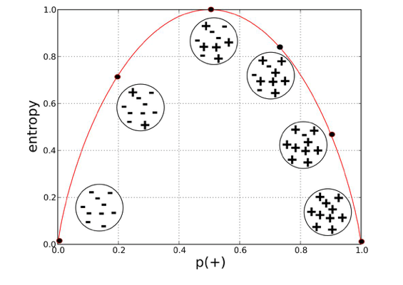
- Entropy = 0: The node is pure (all samples belong to one class).
- Entropy is high: The node contains a mix of different classes, meaning more disorder.
- Entropy is maximized at 0.5: If there is an equal probability of both classes (i.e., 50%-50%), the entropy is at its highest.
Example Calculation:
If a node contains 8 positive examples and 2 negative examples, the entropy is calculated as:
Gini Impurity
Gini Impurity measures how often a randomly chosen element from the set would be incorrectly classified if it were randomly labeled according to the class distribution.
The formula for Gini impurity is:
where:
- is the probability of class in the dataset.
graph TD;
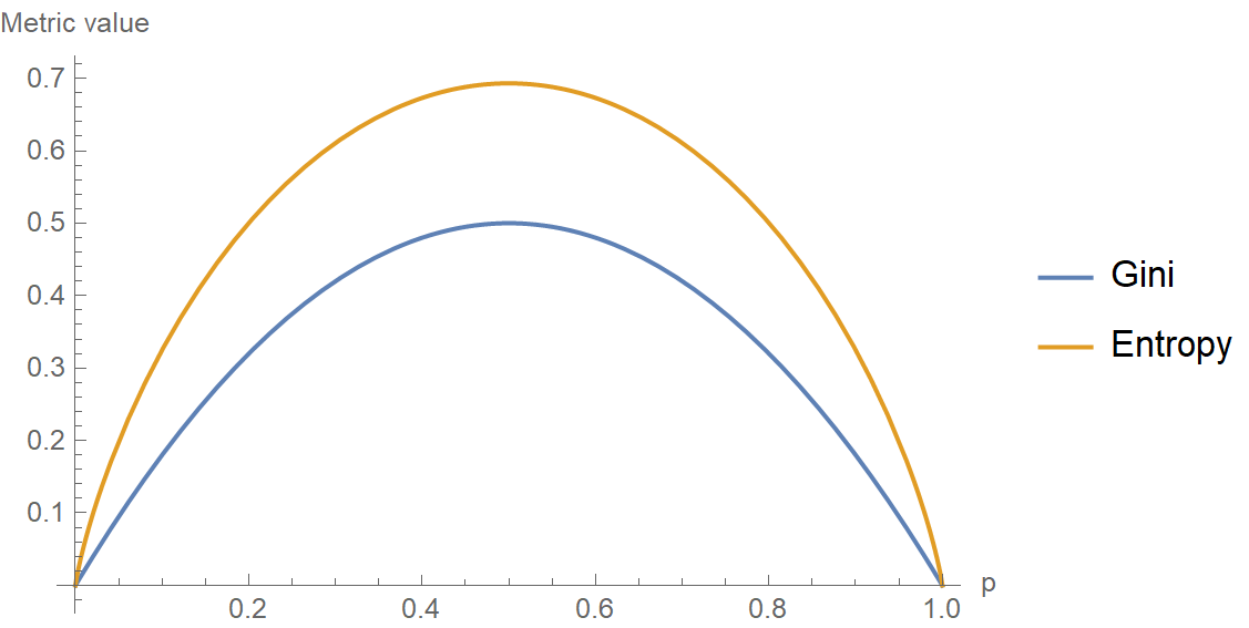
A(Class Distribution) -->|Pure Node| B(Entropy = 0, Gini = 0);
A -->|50-50 Split| C(Entropy = 1, Gini = 0.5);
- Gini = 0: The node is completely pure.
- Gini is high: The node contains a mixture of classes.
Example Calculation:
For the same node with 8 positive and 2 negative examples:
Both metrics are used to determine the best way to split a node in a decision tree, but they have slight differences:
- Entropy is more computationally expensive since it involves logarithmic calculations.
- Gini Impurity is faster to compute and often preferred in decision tree implementations like CART (Classification and Regression Trees).
In practice, both perform similarly, and the choice depends on the specific problem and computational constraints.
By using these metrics, we can quantify the impurity of nodes and use them to decide the best possible splits while constructing a decision tree.
Choosing a Split: Information Gain
When constructing a decision tree, selecting the best feature to split on is crucial for building an optimal model. The goal is to maximize the Information Gain, which measures how well a feature separates the data into pure subsets.
Reducing Entropy
Information Gain (IG) is the reduction in entropy after splitting on a feature. It is calculated as:
where:
- is the entropy of the original set.
- represents subsets created by splitting on attribute .
- is the weighted proportion of samples in each subset.
Example Calculation
Consider a dataset with the following samples:
-
Compute initial entropy:
- 5
Catlabels and 5Doglabels.
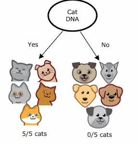
-
, .
-
.
- 5
-
Compute entropy after splitting by
Ear Shape:-
Subset
Pointy: {Cat, Cat, Cat, Cat, Dog} -
Subset
Floppy: {Cat, Dog, Dog, Dog, Dog} -
-
-
Compute entropy after splitting by
Face Shape:-
Subset
Round: {Cat, Cat, Cat, Dog, Dog, Dog, Cat} -
Subset
Not Round: {Cat, Dog, Dog} -
-
-
Compute entropy after splitting by
Whiskers:-
Subset
Present: {Cat, Cat, Cat, Dog} -
Subset
Absent: {Dog, Dog, Dog, Dog, Cat, Cat} -
-
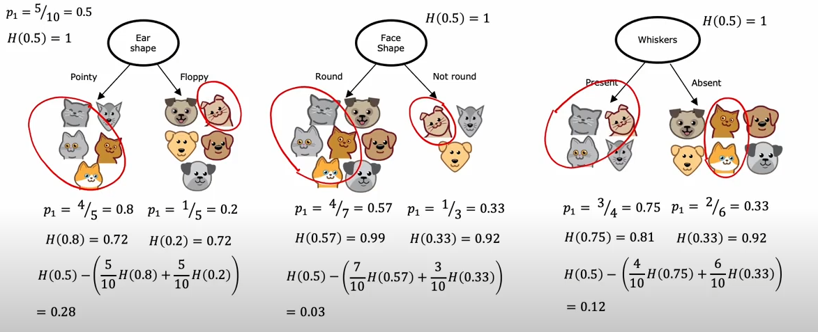
Since the highest Information Gain is (Ear Shape), splitting on either of these features is optimal.
Decision Trees for Continuous Features
When working with continuous features, decision trees can still be used effectively to predict outcomes, just like with categorical features.
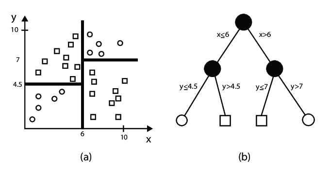
The key difference is that instead of using categorical values for splitting, decision trees for continuous features will determine optimal cutoffs or thresholds in the data. This allows the algorithm to make predictions for continuous target variables based on continuous input features.
In this example, we will predict whether an animal is a cat or dog based on its weight, using a decision tree that handles continuous features.
Let’s say we have the following dataset of animals, and we want to predict if the animal is a cat or dog based on its weight:
| Animal | Weight (kg) |
|---|---|
| Cat | 4.5 |
| Cat | 5.1 |
| Cat | 4.7 |
| Dog | 8.2 |
| Dog | 9.0 |
| Cat | 5.3 |
| Dog | 10.1 |
| Dog | 11.4 |
| Dog | 12.0 |
| Dog | 9.8 |
Here, we aim to build a decision tree based on the Weight feature to determine whether an animal is a cat or a dog.
Step 1: Find the Best Split for the Weight Feature
We will evaluate potential splits based on the Weight feature. The decision tree will consider possible cutoffs and calculate the impurity or variance for each split.
Let’s consider the following splits:
- Weight ≤ 7.0 kg: Assign
Cat - Weight > 7.0 kg: Assign
Dog
The decision tree will evaluate these splits by computing the impurity (for classification) or variance (for regression) for each possible split.
Step 2: Train a Decision Tree Model
We can use a decision tree to learn the best split and predict the animal type based on the weight. Here is how we can implement this in Python:
import numpy as np
from sklearn.tree import DecisionTreeClassifier
import pandas as pd

# Creating the dataset
data = {
    'Weight': [4.5, 5.1, 4.7, 8.2, 9.0, 5.3, 10.1, 11.4, 12.0, 9.8],
    'Animal': ['Cat', 'Cat', 'Cat', 'Dog', 'Dog', 'Cat', 'Dog', 'Dog', 'Dog', 'Dog']
}
df = pd.DataFrame(data)

# Splitting features and target
X = df[['Weight']]  # Feature
y = df['Animal']  # Target

# Training a decision tree classifier
clf = DecisionTreeClassifier(criterion='gini', max_depth=1)
clf.fit(X, y)

# Predicting animal type
predictions = clf.predict(X)
print(f'Predicted Animals: {predictions}')
Step 3: Visualizing the Decision Tree
The decision tree can be visualized to show how the split is made based on the Weight feature.
from sklearn.tree import plot_tree
import matplotlib.pyplot as plt

plt.figure(figsize=(10,8))
plot_tree(clf, feature_names=['Weight'], class_names=['Cat', 'Dog'], filled=True)
plt.show()
Step 4: Interpreting the Results
The resulting decision tree will have a root node where the Weight feature is split at a threshold (e.g., kg). If the animal’s weight is less than or equal to kg, it is classified as a Cat; otherwise, it is classified as a Dog.
Regression Trees
Regression trees are used when the target variable is continuous rather than categorical. Unlike classification trees, which predict discrete labels, regression trees predict numerical values by recursively partitioning the data and assigning an average value to each leaf node.
How Regression Trees Work
- Splitting the Data: The algorithm finds the best feature and threshold to split the data by minimizing variance.
- Assigning Values to Leaves: Instead of class labels, leaf nodes store the mean of the target values in that region.
- Prediction: Given a new sample, traverse the tree based on feature values and return the mean value from the corresponding leaf node.
Example: Predicting Animal Weights
We extend our dataset by adding a new feature: Weight. Our dataset consists of 10 animals, with the following features:
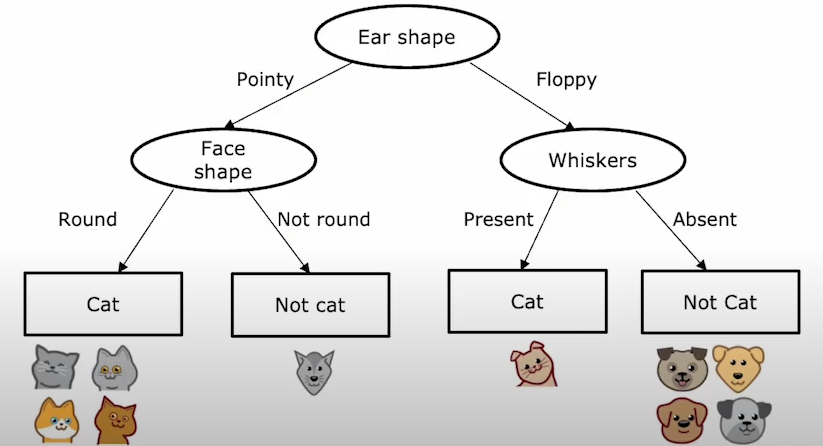
- Ear Shape: (Pointy, Floppy)
- Face Shape: (Round, Not Round)
- Whiskers: (Present, Absent)
- Weight (kg): Continuous target variable
| Ear Shape | Face Shape | Whiskers | Animal | Weight (kg) |
|---|---|---|---|---|
| Pointy | Round | Present | Cat | 4.5 |
| Pointy | Round | Present | Cat | 5.1 |
| Pointy | Round | Absent | Cat | 4.7 |
| Pointy | Not Round | Present | Dog | 8.2 |
| Pointy | Not Round | Absent | Dog | 9.0 |
| Floppy | Round | Present | Cat | 5.3 |
| Floppy | Round | Absent | Dog | 10.1 |
| Floppy | Not Round | Present | Dog | 11.4 |
| Floppy | Not Round | Absent | Dog | 12.0 |
| Floppy | Round | Absent | Dog | 9.8 |
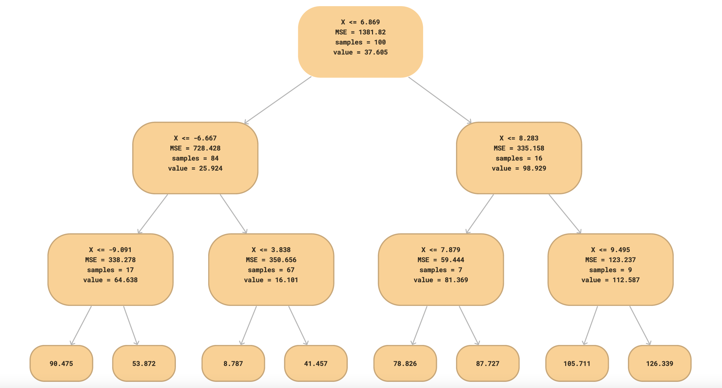
Building a Regression Tree
We use Mean Squared Error (MSE) to determine the best split. The split that results in the lowest MSE is selected.
Step 1: Compute Initial MSE
The overall mean weight is:
MSE before splitting:
Step 2: Find the Best Split
We evaluate splits based on feature values:
-
Split on Ear Shape:
- Pointy: → Mean =
- Floppy: → Mean =
- MSE = (better than initial MSE)
-
Split on Face Shape:
- Round: → Mean =
- Not Round: → Mean =
- MSE = (even better)
-
Split on Whiskers:
- Present: → Mean =
- Absent: → Mean =
- MSE = (better than initial but worse than Face Shape)
Thus, Face Shape is chosen as the first split.
Implementing in Python
import numpy as np
from sklearn.tree import DecisionTreeRegressor
import pandas as pd

# Creating the dataset
data = {
    'Ear_Shape': [0, 0, 0, 0, 0, 1, 1, 1, 1, 1],  # 0: Pointy, 1: Floppy
    'Face_Shape': [0, 0, 0, 1, 1, 0, 0, 1, 1, 0],  # 0: Round, 1: Not Round
    'Whiskers': [0, 0, 1, 0, 1, 0, 1, 1, 0, 0],  # 0: Present, 1: Absent
    'Weight': [4.5, 5.1, 4.7, 8.2, 9.0, 5.3, 10.1, 11.4, 12.0, 9.8]
}
df = pd.DataFrame(data)

# Splitting features and target
X = df[['Ear_Shape', 'Face_Shape', 'Whiskers']]
y = df['Weight']

# Training a regression tree
regressor = DecisionTreeRegressor(criterion='squared_error', max_depth=2)
regressor.fit(X, y)

# Predicting weights
predictions = regressor.predict(X)
print(f'Predicted Weights: {predictions}')
This regression tree provides predictions for the animal weights based on feature values.
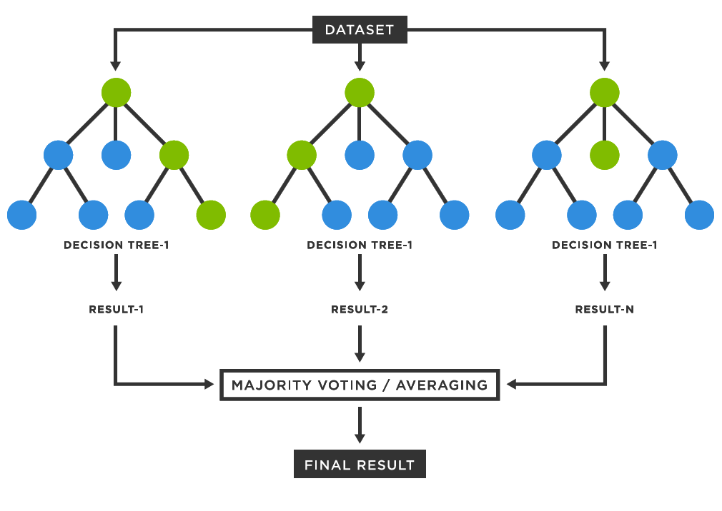
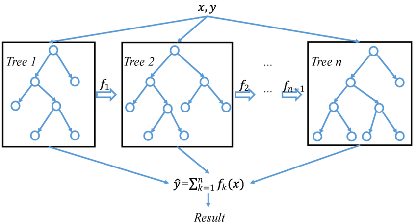
Using Multiple Decision Trees
Using a single decision tree can sometimes lead to overfitting or instability, especially if the dataset has noise. By using multiple decision trees together, we can improve model performance and robustness. Two main techniques to achieve this are Bagging and Boosting.
Bagging (Bootstrap Aggregating)
Bagging reduces variance by training multiple decision trees on different random subsets of the dataset and then averaging their predictions. The most well-known example of bagging is the Random Forest algorithm.
Key Steps in Bagging:
- Draw random subsets (with replacement) from the training data.
- Train a decision tree on each subset.
- Combine predictions using majority voting (for classification) or averaging (for regression).
Visualization of Bagging:
graph TD;
    A[Dataset] -->|Bootstrap Sampling| B1[Tree 1];
    A[Dataset] -->|Bootstrap Sampling| B2[Tree 2];
    A[Dataset] -->|Bootstrap Sampling| B3[Tree 3];
    B1 --> C[Majority Vote];
    B2 --> C;
    B3 --> C;
Sampling with Replacement
Sampling with replacement is a technique where each data point has an equal probability of being selected multiple times in a new sample. This method is widely used in Bootstrap Aggregating (Bagging) to create multiple training datasets from the original dataset, allowing for robust model training and variance reduction.
- Why use Sampling with Replacement?
- It helps in reducing model variance.
- Generates multiple diverse datasets from the original dataset.
- Prevents overfitting by averaging multiple models.
Bootstrap Sampling Process
- Given a dataset of size , create a new dataset by randomly selecting samples with replacement.
- Some original samples may appear multiple times, while others may not appear at all.
- Train multiple models on these sampled datasets and aggregate predictions.
Consider a dataset with five samples :
| Original Data | Bootstrap Sample 1 | Bootstrap Sample 2 |
|---|---|---|
| A | B | A |
| B | A | C |
| C | C | A |
| D | D | B |
| E | A | E |
Notice that in each bootstrap sample, some samples appear multiple times while others are missing.
Random Forest Algorithm
Random Forest is an ensemble learning method that builds multiple decision trees and merges them to achieve better performance. It is based on the concept of bagging (Bootstrap Aggregating), which helps reduce overfitting and improve accuracy.
How Random Forest Works
- Bootstrap Sampling: Randomly select subsets of the training data (with replacement).
- Decision Trees: Train multiple decision trees on different subsets.
- Feature Randomness: At each split, only a random subset of features is considered to introduce diversity.
- Aggregation:
- For classification, it takes a majority vote across all trees.
- For regression, it averages the predictions of all trees.
where is the number of trees and is the prediction of the tree.
Key Hyperparameters
| Hyperparameter | Description |
|---|---|
n_estimators | Number of decision trees in the forest |
max_depth | Maximum depth of each tree |
max_features | Number of features considered for splitting |
min_samples_split | Minimum samples required to split a node |
min_samples_leaf | Minimum samples required in a leaf node |
Decision Tree vs. Random Forest
graph TD;
    A[Dataset] -->|Training| B[Single Decision Tree];
    A -->|Bootstrap Sampling| C[Multiple Decision Trees];
    C -->|Aggregation| D[Final Prediction];
Random Forest example on Telco Customer Churn Dataset
import pandas as pd
import numpy as np
from sklearn.model_selection import train_test_split
from sklearn.ensemble import RandomForestClassifier
from sklearn.metrics import accuracy_score, classification_report

# Load the dataset
df = pd.read_csv('Telco-Customer-Churn.csv')

# Preprocessing
df = df.drop(columns=['customerID'])  # Remove non-relevant column
df = pd.get_dummies(df, drop_first=True)  # Convert categorical variables

# Splitting data
X = df.drop(columns=['Churn_Yes'])
y = df['Churn_Yes']
X_train, X_test, y_train, y_test = train_test_split(X, y, test_size=0.2, random_state=42)

# Train Random Forest model
rf = RandomForestClassifier(n_estimators=100, max_depth=10, random_state=42)
rf.fit(X_train, y_train)

# Predictions
y_pred = rf.predict(X_test)

# Evaluation
print("Accuracy:", accuracy_score(y_test, y_pred))
print(classification_report(y_test, y_pred))
When to Use Random Forest
- When you need high accuracy with minimal tuning.
- When dealing with large feature spaces.
- When feature importance is important.
- When you want to reduce overfitting compared to decision trees.
Random Forest is a powerful and flexible model that performs well across various datasets. However, it can be computationally expensive for large datasets.
Boosting
Boosting is another ensemble method that builds trees sequentially, with each tree trying to correct the mistakes of the previous one. It focuses on difficult examples by assigning them higher weights.
The most popular boosting method is XGBoost (Extreme Gradient Boosting).
Key Steps in Boosting:
- Train a weak model on the training data.
- Identify misclassified samples and assign them higher weights.
- Train the next model focusing on these hard cases.
- Repeat until a stopping criterion is met.
Visualization of Boosting:
graph TD;
    A[Dataset] -->|Train Weak Model| B1[Tree 1];
    B1 -->|Adjust Weights| B2[Tree 2];
    B2 -->|Adjust Weights| B3[Tree 3];
    B3 --> C[Final Prediction];
XGBoost
XGBoost (Extreme Gradient Boosting) is a powerful and efficient implementation of gradient boosting that is widely used in machine learning competitions and real-world applications due to its high performance and scalability.
XGBoost builds an ensemble of decision trees sequentially, where each tree corrects the errors of the previous ones. The algorithm optimizes a loss function using gradient descent, allowing it to minimize errors effectively.
Key Components of XGBoost:
- Gradient Boosting Framework: Uses boosting to improve weak learners iteratively.
- Regularization: Includes L1 and L2 regularization to reduce overfitting.
- Parallelization: Optimized for fast training using parallel computing.
- Handling Missing Values: Automatically finds optimal splits for missing data.
- Tree Pruning: Uses depth-wise pruning instead of weight pruning for efficiency.
- Custom Objective Functions: Allows defining custom loss functions.
XGBoost optimizes the following objective function:
Where:
- is the loss function (e.g., squared error for regression, log loss for classification).
- is the regularization term controlling model complexity.
- represents individual trees.
Implementing XGBoost on Telco Customer Churn Dataset
We will train an XGBoost model to predict customer churn.
Step 1: Load the dataset
import pandas as pd
from xgboost import XGBClassifier
from sklearn.model_selection import train_test_split
from sklearn.metrics import accuracy_score

# Load dataset
df = pd.read_csv("Telco-Customer-Churn.csv")

# Preprocess data
df = df.dropna()
df = pd.get_dummies(df, drop_first=True)

X = df.drop("Churn_Yes", axis=1)
y = df["Churn_Yes"]

# Split data
X_train, X_test, y_train, y_test = train_test_split(X, y, test_size=0.2, random_state=42)
Step 2: Train the XGBoost Model
xgb_model = XGBClassifier(n_estimators=100, learning_rate=0.1, max_depth=4, reg_lambda=1, use_label_encoder=False, eval_metric='logloss')
xgb_model.fit(X_train, y_train)
Step 3: Evaluate the Model
y_pred = xgb_model.predict(X_test)
accuracy = accuracy_score(y_test, y_pred)
print(f"Accuracy: {accuracy:.4f}")
Hyperparameter Tuning
Key hyperparameters in XGBoost:
| Hyperparameter | Description |
|---|---|
n_estimators | Number of trees in the model. |
learning_rate | Step size for updating weights. |
max_depth | Maximum depth of trees. |
subsample | Fraction of samples used per tree. |
colsample_bytree | Fraction of features used per tree. |
gamma | Minimum loss reduction required for split. |
When to Use XGBoost
- When you have structured/tabular data.
- When you need high accuracy.
- When you need a model that handles missing values efficiently.
- When feature interactions are important.
XGBoost is one of the most powerful algorithms for predictive modeling. By leveraging its strengths in handling structured data, regularization, and parallel processing, it can significantly outperform traditional machine learning methods in many real-world applications.
XGBoost vs Random Forest
| Feature | XGBoost | Random Forest |
|---|---|---|
| Training Speed | Faster (parallelized) | Slower |
| Overfitting Control | Stronger (Regularization) | Moderate |
| Performance on Structured Data | High | Good |
| Handles Missing Data | Yes | No |