Implementation of Forward Propagation
- Coffee Roasting Example (Classification Task)
- Neural Network Architecture
- TensorFlow Implementation
- Forward Propagation Step-by-Step (NumPy Implementation)
- Artificial General Intelligence (AGI)
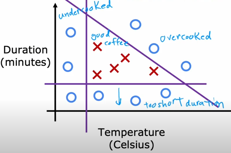
Coffee Roasting Example (Classification Task)
Imagine we want to classify coffee as either “Good” or “Bad” based on two factors:
- Temperature (°C)
- Roasting Time (minutes)
For simplicity, we define:
- Good coffee: If the temperature is between 190°C and 210°C and the roasting time is between 10 and 15 minutes.
- Bad coffee: Any other condition.
We collect the following data:
| Temperature (°C) | Roasting Time (min) | Quality (1 = Good, 0 = Bad) |
|---|---|---|
| 200 | 12 | 1 |
| 180 | 10 | 0 |
| 210 | 15 | 1 |
| 220 | 20 | 0 |
| 195 | 13 | 1 |
We will implement a simple neural network using TensorFlow to classify new coffee samples.
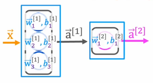
Neural Network Architecture
We construct a neural network using the following structure:
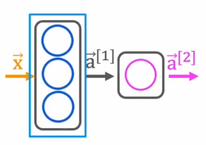
- Input Layer: Two neurons (temperature, time)
- Hidden Layer: Three neurons, activated with the sigmoid function
- Output Layer: One neuron, activated with the sigmoid function (binary classification)
TensorFlow Implementation
Step 1: Importing Libraries
import tensorflow as tf
import numpy as np
tensorflowis the core deep learning library that allows us to define and train neural networks.numpyis used for handling arrays and numerical operations efficiently.
Step 2: Defining Inputs and Outputs
X = np.array([[200, 12], [180, 10], [210, 15], [220, 20], [195, 13]], dtype=np.float32)
y = np.array([[1], [0], [1], [0], [1]], dtype=np.float32)
Xrepresents the input features (temperature and roasting time) as a NumPy array.yrepresents the expected output (1 for good coffee, 0 for bad coffee).dtype=np.float32ensures numerical stability and compatibility with TensorFlow.
Step 3: Building the Model
model = tf.keras.Sequential([
    tf.keras.layers.Dense(3, activation='sigmoid', input_shape=(2,)),
    tf.keras.layers.Dense(1, activation='sigmoid')
])
Sequential()creates a linear stack of layers.Dense(3, activation='sigmoid', input_shape=(2,))defines the hidden layer:- 3 neurons
- Sigmoid activation function
- Input shape of (2,) since we have two input features.
Dense(1, activation='sigmoid')defines the output layer with 1 neuron and sigmoid activation.
Step 4: Training the Model
model.compile(optimizer='adam', loss='binary_crossentropy', metrics=['accuracy'])
model.fit(X, y, epochs=500, verbose=0)
compile()configures the model for training:adamoptimizer adapts the learning rate automatically.binary_crossentropyis used for binary classification problems.accuracymetric tracks how well the model classifies coffee samples.
fit(X, y, epochs=500, verbose=0)trains the model for 500 epochs (iterations over data).
Step 5: Making Predictions
new_coffee = np.array([[205, 14]], dtype=np.float32)
prediction = model.predict(new_coffee)
print("Prediction (Probability of Good Coffee):", prediction)
new_coffeecontains a new sample (205°C, 14 min) to classify.model.predict(new_coffee)computes the probability of the coffee being good.- The output is a probability (closer to 1 means good, closer to 0 means bad).
Forward Propagation Step-by-Step (NumPy Implementation)
We now implement forward propagation manually using NumPy to understand how TensorFlow executes it under the hood.
Initializing Weights and Biases
np.random.seed(42)  # For reproducibility
W1 = np.random.randn(2, 4)  # Weights for hidden layer (2 inputs -> 4 neurons)
b1 = np.random.randn(4)     # Bias for hidden layer
W2 = np.random.randn(4, 1)  # Weights for output layer (4 neurons -> 1 output)
b2 = np.random.randn(1)     # Bias for output layer
np.random.randn()initializes weights and biases randomly from a normal distribution.W1andb1define the hidden layer parameters.W2andb2define the output layer parameters.
Forward Propagation Calculation
def sigmoid(z):
    return 1 / (1 + np.exp(-z))
- This function applies the sigmoid activation function, which outputs values between 0 and 1.
def forward_propagation(X):
    Z1 = np.dot(X, W1) + b1  # Linear transformation (Hidden Layer)
    A1 = sigmoid(Z1)  # Activation function (Hidden Layer)
    Z2 = np.dot(A1, W2) + b2  # Linear transformation (Output Layer)
    A2 = sigmoid(Z2)  # Activation function (Output Layer)
    return A2
np.dot(X, W1) + b1computes the weighted sum of inputs for the hidden layer.sigmoid(Z1)applies the activation function to introduce non-linearity.np.dot(A1, W2) + b2computes the weighted sum of outputs from the hidden layer.sigmoid(Z2)produces the final prediction.
# Testing with an example input
output = forward_propagation(np.array([[185, 10]]))
print(output)
This manually replicates TensorFlow’s forward propagation but using pure NumPy.
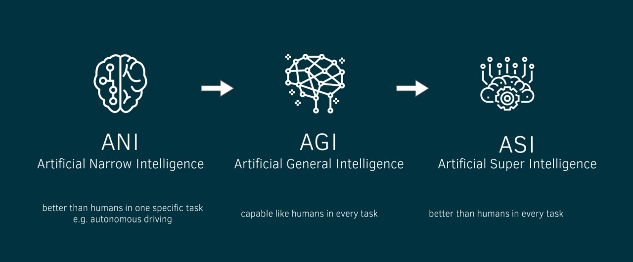
Artificial General Intelligence (AGI)
AGI refers to AI that can perform any intellectual task a human can. Unlike current AI systems, AGI would adapt, learn, and generalize across different tasks without needing task-specific training.
Everyday Example: AGI vs. Narrow AI
- Narrow AI (Current AI): A chess-playing AI can defeat world champions but cannot drive a car.
- AGI: If a chess-playing AI was truly intelligent, it would learn how to drive just like a human without explicit programming.
Key Challenges in AGI
- Transfer Learning: Current AI requires large amounts of data. Humans learn with few examples.
- Common Sense Reasoning: AI struggles with simple logic like “If I drop a glass, it will break.”
- Self-Learning: AGI must improve without needing human intervention.
Is AGI Possible?
- Some scientists believe AGI is decades away, while others argue it may never happen.
- Brain-inspired architectures (like Neural Networks) might be a stepping stone toward AGI.