Reinforcement Learning
- What is Reinforcement Learning?
- Markov Decision Process (MDP)
- State-Action Value Function ()
- Bellman Equation
- Stochastic Environment (Randomness in RL)
- Continuous State vs. Discrete State
- Lunar Lander Example
- -Greedy Policy
- Mini-Batch Learning in Reinforcement Learning
What is Reinforcement Learning?
Reinforcement Learning (RL) is a machine learning paradigm where an agent learns to make sequential decisions by interacting with an environment to maximize a cumulative reward. Unlike supervised learning, where labeled data is provided, RL relies on trial and error, receiving feedback in the form of rewards or penalties.
Key Characteristics of Reinforcement Learning:
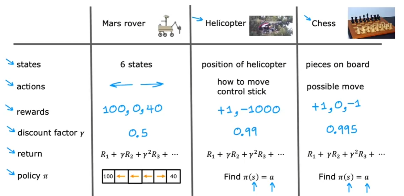
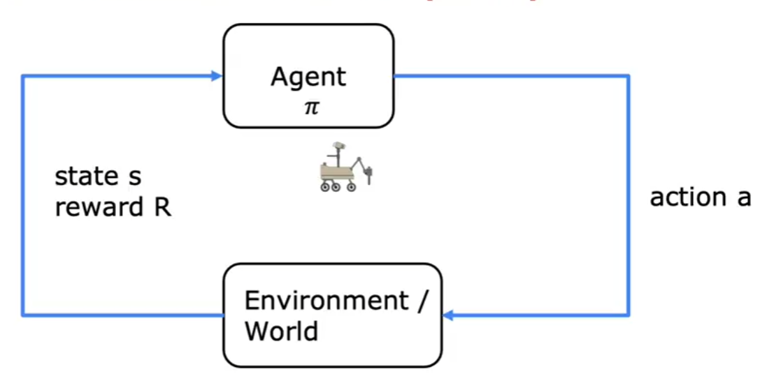
- Agent: The entity making decisions (e.g., a robot, a self-driving car, or an AI player in a game).
- Environment: The external system with which the agent interacts.
- State (s): A representation of the current situation of the agent in the environment.
- Action (a): A choice made by the agent at a given state.
- Reward (R): A numerical value given to the agent as feedback for its actions.
- Policy ( ): A strategy that maps states to actions.
- Return (G): The cumulative reward collected over time.
- Discount Factor ( ): A value between 0 and 1 that determines the importance of future rewards.
Mars Rover Example
Let’s illustrate RL concepts using a Mars Rover example. Imagine a rover exploring a 1D terrain with six grid positions:
Each position is numbered from 1 to 6. The rover starts at position 4, and it can move left (-1) or right (+1). The goal is to maximize its rewards, which are given at positions 1 and 6:
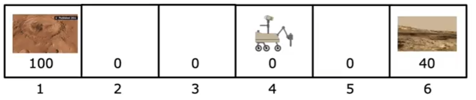
- Position 1 reward: 100 (e.g., a research station with supplies)
- Position 6 reward: 40 (e.g., a safe resting point)
- Other positions reward: 0
States, Actions, and Rewards
| State | Possible Actions | Reward |
|---|---|---|
| 1 | Move right (+1) | 100 |
| 2 | Move left (-1), Move right (+1) | 0 |
| 3 | Move left (-1), Move right (+1) | 0 |
| 4 (Start) | Move left (-1), Move right (+1) | 0 |
| 5 | Move left (-1), Move right (+1) | 0 |
| 6 | Move left (-1) | 40 |
- The agent (rover) must decide which direction to move.
- The state is the current position of the rover.
- The action is moving left or right.
- The reward depends on reaching the goal states (1 or 6).
How the Rover Decides Where to Go
The rover’s decision is based on maximizing its expected future rewards. Since it has two possible goal positions (1 and 6), it must evaluate different strategies. The rover should consider the following:
-
Immediate Reward Strategy
- If the rover focuses only on immediate rewards, it will move randomly, as most positions (except 1 and 6) have a reward of 0.
- This strategy is not optimal because it doesn’t take future rewards into account.
-
Short-Term Greedy Strategy
- If the rover chooses the nearest reward, it will likely go to position 6 since it’s closer than position 1.
- However, this might not be the best long-term decision.
-
Long-Term Reward Maximization
- The rover must evaluate how much discounted future reward it can accumulate.
- Even though position 6 has a reward of 40, position 1 has a much higher reward (100).
- If the rover can reliably reach position 1, it should favor this route, even if it takes more steps.
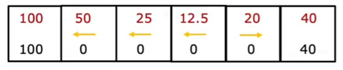
To formalize this, the rover can compute the expected return G for each possible path, considering the discount factor ().
Discount Factor () and Expected Return
The discount factor determines how much future rewards are valued relative to immediate rewards. If , all future rewards are considered equally important. If , future rewards are slightly less important than immediate rewards.
For example, if the rover follows a path where it expects to reach position 1 in 3 steps and receive 100 reward, the discounted return is:
If it reaches position 6 in 2 steps and receives 40 reward, the return is:
Since 72.9 is greater than 32.4, the rover should prioritize going to position 1, even though it is farther away.
Policy ()
A policy () defines the strategy of the rover: for each state, it dictates which action to take. Possible policies include:
- Greedy policy: Always moves towards the highest reward state immediately.
- Exploratory policy: Sometimes tries new actions to find better strategies.
- Discounted return policy: Balances short-term and long-term rewards.
If the rover follows an optimal policy, it should compute the total expected reward for every possible action and pick the one that maximizes its long-term return.
Markov Decision Process (MDP)
Reinforcement Learning problems are often modeled as Markov Decision Processes (MDPs), which are defined by:
- Set of States (S):
- Set of Actions (A):
- Transition Probability (P): Probability of moving from one state to another given an action
- Reward Function (R): Defines the reward received when moving from to
- Discount Factor (): Determines the importance of future rewards.
In our Mars Rover example:
- States (S): {1, 2, 3, 4, 5, 6}
- Actions (A): {Left (-1), Right (+1)}
- Transition Probabilities (P): Deterministic (e.g., if the rover moves right, it always reaches the next state)
- Reward Function (R):
- , ,
- Discount Factor (): (assumed)
State-Action Value Function ()
The State-Action Value Function, denoted as , represents the expected return when starting from state , taking action , and then following a policy . Formally:
This function helps the agent determine which action will lead to the highest reward in a given state.
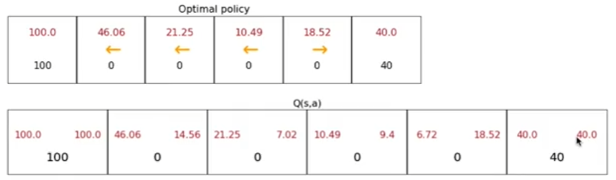
Applying to Mars Rover
Using our Mars rover example, we can estimate values for each state-action pair. Suppose:
The rover should always select the action with the highest value to maximize rewards.
Bellman Equation
The Bellman Equation provides a recursive relationship for computing value functions in reinforcement learning. It expresses the value of a state in terms of the values of successor states.
Understanding the Bellman Equation
In reinforcement learning, an agent makes decisions in a way that maximizes future rewards. However, since future rewards are uncertain, we need a way to estimate them efficiently. The Bellman equation helps us do this by breaking down the value of a state into two components:
- Immediate Reward (): The reward received by taking action in state .
- Future Rewards (): The expected value of the next state , weighted by the probability of reaching that state.
The Bellman equation is written as:
where:
- : The value of state .
- : The immediate reward for taking action in state .
- : The discount factor (), which determines how much future rewards are considered.
- : The probability of reaching state after taking action .
- : The value of the next state .
Example Calculation for Mars Rover
Let’s assume:
- Moving from
4to3has a reward of-1. - Moving from
4to5has a reward of-1. - Position
1has a reward of100.
For :
If we assume and , and a discount factor , we compute:
Thus, the optimal value for state 4 is 44, meaning the agent should prefer moving left toward 3.
Intuition Behind the Bellman Equation
- The Bellman equation decomposes the value of a state into its immediate reward and the expected future reward.
- It allows us to compute values iteratively: we start with rough estimates and refine them over time.
- It helps in policy evaluation—determining how good a given policy is.
- It forms the foundation for Dynamic Programming methods like Value Iteration and Policy Iteration.
Stochastic Environment (Randomness in RL)
In real-world applications, environments are often stochastic, meaning actions do not always lead to the same outcome.
Stochasticity in the Mars Rover Example
Suppose the Mars rover’s motors sometimes malfunction, causing it to move in the opposite direction with a small probability (e.g., 10% of the time). Now, the transition dynamics include:
This randomness makes decision-making more challenging. Instead of just considering rewards, the rover must now account for expected rewards and the probability of ending up in different states.
Impact on Decision-Making
With stochastic environments, deterministic policies (always taking the best action) may not be optimal. Instead, an exploration-exploitation balance is needed:
- Exploitation: Following the best-known action based on past experience.
- Exploration: Trying new actions to discover potentially better rewards.
This concept is central to algorithms like Q-Learning and Policy Gradient Methods, which we will discuss in future sections.
Continuous State vs. Discrete State
In reinforcement learning, states can be either discrete or continuous. A discrete state means that the number of possible states is finite and well-defined, whereas a continuous state implies an infinite number of possible states.
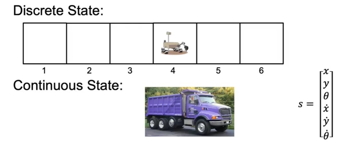
For example, consider our Mars Rover example with six possible states. The rover can be in any one of these six states at any given time, making it a discrete state environment. However, if we consider a truck driving on a highway, its position, speed, angle, and other attributes can take an infinite number of values, making it a continuous state environment.
Continuous state spaces are often approximated using function approximators like neural networks to generalize over an infinite number of states efficiently.
Lunar Lander Example
A classic reinforcement learning problem is the Lunar Lander, where the objective is to safely land a spacecraft on the surface of a planet. The agent (lander) interacts with the environment by selecting one of four possible actions:
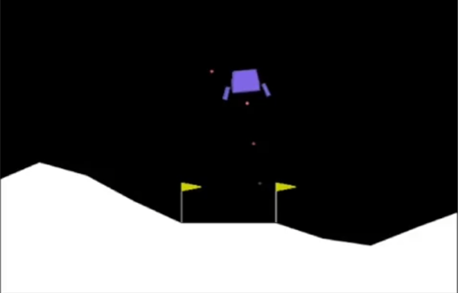
- Do Nothing: No thrust is applied.
- Left Thruster: Applies force to move left.
- Right Thruster: Applies force to move right.
- Main Thruster: Applies force to slow descent.
Rewards and Penalties:
The environment provides feedback through rewards and penalties:
- Soft Landing: +100 reward
- Crash Landing: -100 penalty
- Firing Main Engine: -0.3 penalty (fuel consumption)
- Firing Side Thrusters: -0.1 penalty (fuel consumption)
State Representation
The state of the lunar lander can be represented as:
where:
- : Position of the lander
- : Orientation (tilt angle)
- : Contact with left and right landing pads (binary values)
- : Velocities in x and y directions
- : Angular velocity
The policy function determines which action to take given the current state.
Deep Q-Network (DQN) Neural Network for Lunar Lander
To approximate the optimal policy, we use a deep neural network. The network takes the 8-dimensional state vector as input and predicts Q-values for each of the four actions.
Network Architecture:
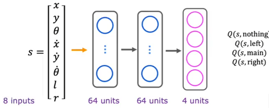
- Input Layer (8 neurons): Corresponds to
- Two Hidden Layers (64 neurons each, ReLU activation)
- Output Layer (4 neurons): Represents the Q-values for the four possible actions
The output neurons correspond to:
The network is trained using the Bellman equation to minimize the difference between predicted and actual Q-values.
-Greedy Policy
In reinforcement learning, an agent must balance exploration (trying new actions) and exploitation (choosing the best-known action). The -greedy policy is a common approach to achieve this balance:
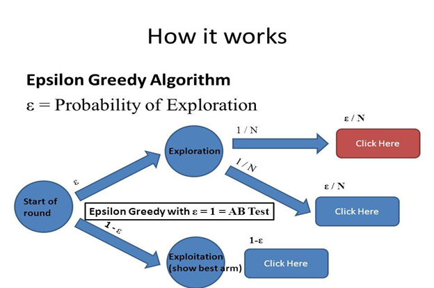
- With probability , take a random action (exploration).
- With probability , take the action with the highest Q-value (exploitation).
Initially, is set to a high value (e.g., 1.0) to encourage exploration and gradually decays over time.
Mini-Batch Learning in Reinforcement Learning
In deep reinforcement learning, we use mini-batch learning to improve training efficiency and stability.
Why Mini-Batch Learning?
- Prevents large updates from a single experience (stabilizes training).
- Helps break the correlation between consecutive experiences (improves generalization).
- Allows efficient GPU computation (faster convergence).
How It Works:
- Store experiences (state, action, reward, next state) in a replay buffer.
- Sample a mini-batch of experiences.
- Compute target Q-values using the Bellman equation.
- Perform a gradient descent update on the Q-network.
Mini-batch learning makes reinforcement learning more robust and prevents overfitting to recent experiences.