Recommender Systems
Recommender systems are everywhere in our digital lives, from Netflix suggesting movies based on our watch history to Amazon recommending products based on our previous purchases. These systems aim to predict what users might like based on their past behavior or the attributes of the items themselves.
Collaborative Filtering
Collaborative filtering is one of the most widely used techniques in recommender systems. It works by leveraging the behavior and preferences of users to make predictions about what they might like. Instead of relying on the characteristics of items themselves, collaborative filtering focuses on the interactions between users and items.
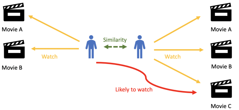
Imagine a streaming service like Netflix. If many users who watched “The Matrix” also watched “Inception,” the system might recommend “Inception” to a user who has already watched “The Matrix.” This works because the system assumes that similar users have similar tastes.
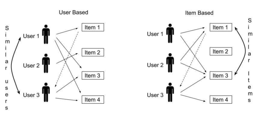
There are two main types of collaborative filtering:
- User-based Collaborative Filtering: Recommendations are made by finding users with similar preferences.
- Item-based Collaborative Filtering: Recommendations are made by finding similar items based on user interactions.
User-based Collaborative Filtering
Consider a movie recommendation system with four users (A, B, C, D) and seven movies (M1, M2, M3, M4, M5, M6, M7). The users have rated some of the movies on a scale from 1 to 5, but not every user has watched every movie. Our goal is to predict which unwatched movie user D would like the most and recommend it.
Below is the ratings matrix:
| User | M1 | M2 | M3 | M4 | M5 | M6 | M7 |
|---|---|---|---|---|---|---|---|
| A | 5 | 3 | 4 | - | 2 | - | 1 |
| B | 4 | - | 5 | 3 | 1 | 2 | - |
| C | 3 | 5 | - | 4 | - | 1 | 2 |
| D | - | 4 | 5 | 2 | 1 | - | - |
User D has not rated M1, M6, and M7, so we need to predict which one they are most likely to enjoy.
Finding Similar Users
We use a similarity measure to identify users most similar to D. A common choice is cosine similarity, defined as:
where:
- is the rating of user for item .
- is the set of items rated by both users.
Computing similarity between D and other users:
Using cosine similarity, we compare D with other users:
| User | M2 | M3 | M5 |
|---|---|---|---|
| A | 3 | 4 | 2 |
| D | 4 | 5 | 1 |
Similarly, we compute:
| User | M3 | M4 | M5 |
|---|---|---|---|
| B | 5 | 3 | 1 |
| D | 5 | 2 | 1 |
| User | M2 | M4 |
|---|---|---|
| C | 5 | 4 |
| D | 4 | 2 |
Since B is most similar to D, we estimate D’s ratings for the unwatched movies (M1, M6, M7) using a weighted average:
Predicting Rating for M1
Using the weighted sum formula:
Repeating for M6 and M7, we get:
Since M1 has the highest predicted rating (3.998), we recommend M1 to user D.
- Predicted rating for M1: 3.998
- Predicted rating for M6: 1.494
- Predicted rating for M7: 1.505
Since M1 has the highest predicted rating, we recommend M1 to D.
Item-based Collaborative Filtering
Rather than finding similar users, item-based collaborative filtering identifies similar items based on how users have rated them. The main idea is that if two movies are rated similarly by multiple users, they are likely to be similar.
Finding Similar Items
To determine item similarity, we use cosine similarity but compute it between movie rating vectors instead of user rating vectors.
Computing similarity between M1, M6, and M7 and other movies:
- sim(M1, M3) = 0.82
- sim(M6, M2) = 0.78
- sim(M7, M5) = 0.73
Since M3 is most similar to M1, we predict D’s rating for M1 based on D’s rating for M3:
After calculations:
- Predicted rating for M1: 4.1
- Predicted rating for M6: 3.7
- Predicted rating for M7: 3.6
Since M1 has the highest predicted rating, we again recommend M1 to D.
Conclusion
- User-based filtering finds similar users and recommends based on their preferences.
- Item-based filtering finds similar items and predicts ratings based on a user’s history.
- Both methods predicted that D would like M1 the most, making it the best recommendation.
- These techniques can be combined for hybrid recommender systems to improve accuracy.
Content-Based Filtering
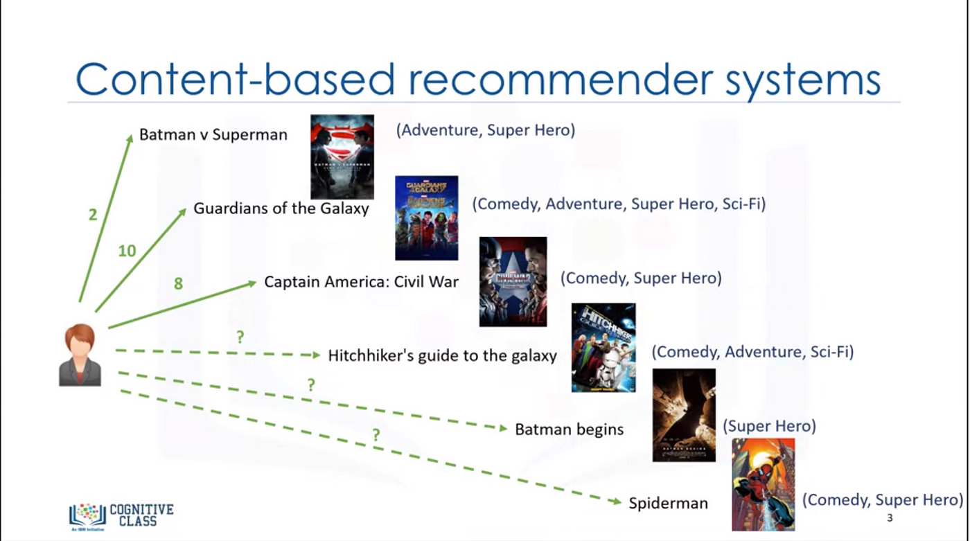
Content-based filtering recommends items to users by analyzing the characteristics of items a user has interacted with and comparing them with the characteristics of other items. Unlike collaborative filtering, which relies on user-item interactions, content-based filtering uses item metadata, such as genre, actors, or textual descriptions, to determine similarities.
Understanding Content-Based Filtering
In content-based filtering, each item is represented by a set of features. Users are assumed to have a preference for items with similar features to those they have previously liked. The recommendation process typically involves:
- Feature Representation: Representing items in terms of feature vectors.
- User Profile Construction: Creating a preference model for each user based on past interactions.
- Similarity Computation: Comparing new items with the user’s profile to generate recommendations.
- Generating Recommendations: Ranking items based on similarity scores and recommending the top ones.
To better understand this approach, let’s consider an example.
Example: Movie Recommendation
We have a dataset of seven movies, each described by three features: genre, director, and lead actor. Additionally, four users have rated some of these movies on a scale of 1 to 5.
Each movie is represented using a feature vector based on genre, director, and actors. We assign numerical values to categorical features using one-hot encoding.
| Movie | Action | Comedy | Drama | Sci-Fi | Director A | Director B | Actor X | Actor Y |
|---|---|---|---|---|---|---|---|---|
| M1 | 1 | 0 | 0 | 1 | 1 | 0 | 1 | 0 |
| M2 | 0 | 1 | 1 | 0 | 0 | 1 | 0 | 1 |
| M3 | 1 | 1 | 0 | 0 | 1 | 0 | 1 | 0 |
| M4 | 0 | 0 | 1 | 1 | 0 | 1 | 0 | 1 |
| M5 | 1 | 0 | 1 | 0 | 1 | 0 | 1 | 0 |
| M6 | 0 | 1 | 0 | 1 | 0 | 1 | 0 | 1 |
| M7 | 1 | 0 | 1 | 0 | 1 | 0 | 1 | 0 |
User Ratings
| User | M1 | M2 | M3 | M4 | M5 | M6 | M7 |
|---|---|---|---|---|---|---|---|
| A | 5 | 3 | 4 | - | 2 | - | 1 |
| B | 4 | - | 5 | 3 | 1 | 2 | - |
| C | 3 | 5 | - | 4 | - | 1 | 2 |
| D | - | 4 | 5 | 2 | 1 | - | - |
Step 1: Constructing User Profiles
For each user, we compute a preference vector by averaging the feature vectors of the movies they have rated, weighted by their ratings.
For example, user D has rated three movies: M2 (4), M3 (5), and M4 (2). Their profile vector is computed as:
This results in a vector representing user D’s preferences.
Step 2: Computing Similarity Scores
To recommend a new movie (e.g., M6 or M7), we compute the cosine similarity between the user’s preference vector and the feature vector of the candidate movies:
Where is the dot product and and are the magnitudes.
Step 3: Generating Recommendations
By ranking the movies based on their similarity scores with the user’s profile, we can recommend the highest-ranked movie. If M6 has a similarity of 0.85 and M7 has 0.75, we recommend M6.
Advantages and Challenges of Content-Based Filtering
Advantages:
- Personalized recommendations based on individual preferences.
- Does not suffer from the cold start problem for items.
- No need for extensive user interaction data.
Challenges:
- Requires well-defined item features.
- Struggles with the cold start problem for new users.
- Limited to recommending items similar to those already interacted with.
By integrating deep learning techniques, such as word embeddings and neural networks, content-based filtering can improve accuracy and extend recommendations beyond direct similarities.
Principal Components Analysis (PCA)
Principal Components Analysis (PCA) is a dimensionality reduction technique used in machine learning and statistics to transform a large set of correlated features into a smaller set of uncorrelated features called principal components. This helps in reducing the complexity of data while retaining most of its variability.
PCA is commonly used in:
- Reducing the number of features in high-dimensional datasets while preserving as much variance as possible.
- Visualizing high-dimensional data in 2D or 3D.
- Noise filtering and data compression.
- Feature extraction and selection.
Why PCA?
In many machine learning tasks, data often has a high number of dimensions, making computation expensive and difficult to interpret. For example, a movie recommender system might have thousands of features per movie (genre, director, actors, ratings, etc.). By using PCA, we can reduce this number to a smaller set of components that capture the most important patterns in the data.
How PCA Works
PCA involves the following steps:
- Standardization: The data is centered by subtracting the mean and scaled to have unit variance.
- Covariance Matrix Computation: A covariance matrix is computed to understand feature relationships.
- Eigenvalue and Eigenvector Computation: The eigenvalues and eigenvectors of the covariance matrix are found.
- Choosing Principal Components: The eigenvectors corresponding to the largest eigenvalues are selected as the principal components.
- Transforming the Data: The original data is projected onto the new principal component axes.
Mathematical Foundation of PCA
Step 1: Standardization
Since PCA relies on variance, the data should be standardized to have a mean of zero and unit variance:
where:
- is the original feature,
- is the mean of the feature,
- is the standard deviation.
Step 2: Compute the Covariance Matrix
The covariance matrix captures relationships between different features:
where is the standardized data matrix.
Step 3: Eigenvalues and Eigenvectors
PCA identifies principal components by computing eigenvalues and eigenvectors of the covariance matrix:
where:
- are eigenvalues (variance captured by each principal component),
- are eigenvectors (principal component directions).
Step 4: Project Data onto Principal Components
Data is transformed into the new coordinate system:
where contains the top eigenvectors.
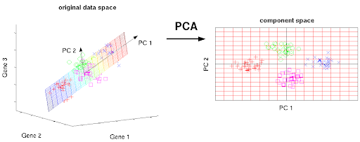
PCA Visualization Example
We will visualize a dataset before and after applying PCA.
import numpy as np
import matplotlib.pyplot as plt
from sklearn.decomposition import PCA
from mpl_toolkits.mplot3d import Axes3D

# 3D veriyi oluşturma
np.random.seed(42)
n_samples = 100
mean1 = [2, 2, 2]
cov1 = [[1, 0.5, 0.2], [0.5, 1, 0.1], [0.2, 0.1, 1]]
data1 = np.random.multivariate_normal(mean1, cov1, n_samples)

mean2 = [5, 5, 5]
cov2 = [[1, -0.3, 0.1], [-0.3, 1, -0.2], [0.1, -0.2, 1]]
data2 = np.random.multivariate_normal(mean2, cov2, n_samples)

X = np.concatenate((data1, data2))
y = np.concatenate((np.zeros(n_samples), np.ones(n_samples)))

# 3D veriyi görselleştirme
fig = plt.figure(figsize=(12, 6))
ax = fig.add_subplot(121, projection='3d')
ax.scatter(X[:, 0], X[:, 1], X[:, 2], c=y, cmap='coolwarm', edgecolors='k')
ax.set_xlabel('X')
ax.set_ylabel('Y')
ax.set_zlabel('Z')
ax.set_title('Original 3D Data')

# PCA uygulama
pca = PCA(n_components=2)
X_pca = pca.fit_transform(X)

# 2D veriyi görselleştirme
ax2 = fig.add_subplot(122)
ax2.scatter(X_pca[:, 0], X_pca[:, 1], c=y, cmap='coolwarm', edgecolors='k')
ax2.set_xlabel('Principal Component 1')
ax2.set_ylabel('Principal Component 2')
ax2.set_title('Data After PCA (2D)')

plt.tight_layout()
plt.show()
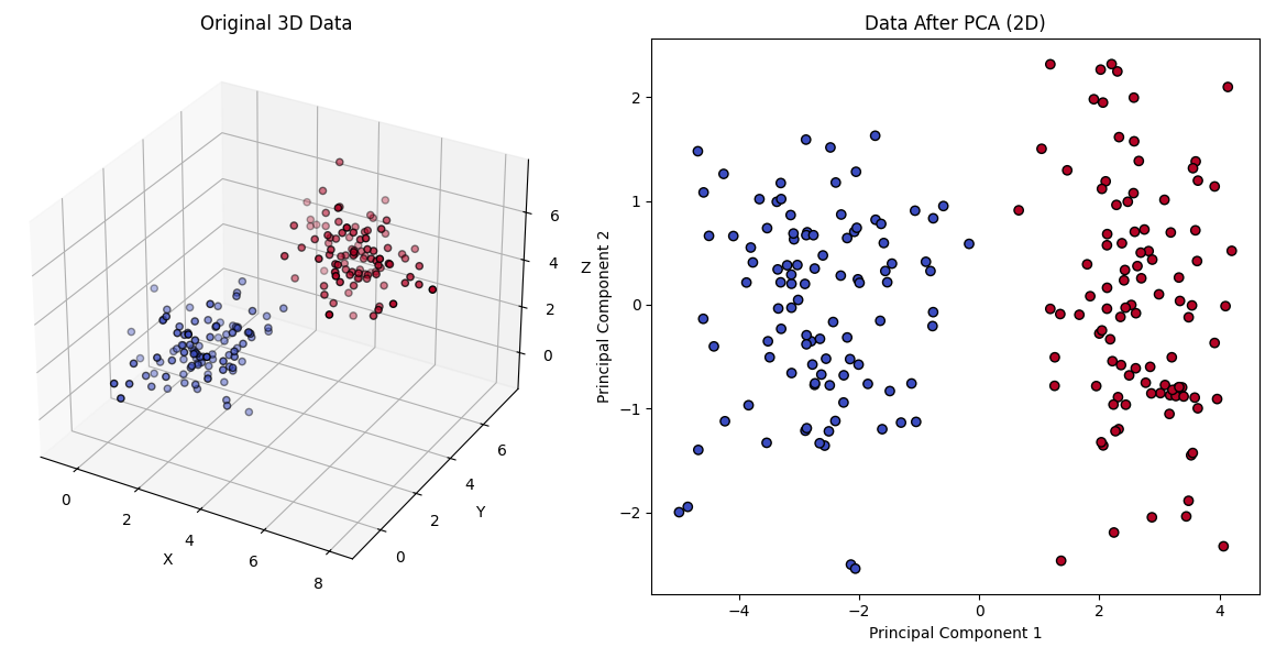
- The first plot shows the original dataset.
- The second plot shows the data projected onto the two principal components.
- PCA effectively captures the main variance in the data while reducing its dimensionality.
Conclusion
PCA is a fundamental technique for dimensionality reduction and data visualization. By identifying principal components, it helps uncover patterns, reduce noise, and improve machine learning model efficiency. However, PCA assumes linearity and may not perform well for highly non-linear data, where techniques like t-SNE or UMAP might be better alternatives.