Anomaly Detection
- Finding Unusual Events
- Gaussian (Normal) Distribution
- Anomaly Detection Algorithm
- Developing and Evaluating an Anomaly Detection System
- 5. Anomaly Detection vs. Supervised Learning
- Choosing What Features to Use
- Full Python Example with TensorFlow
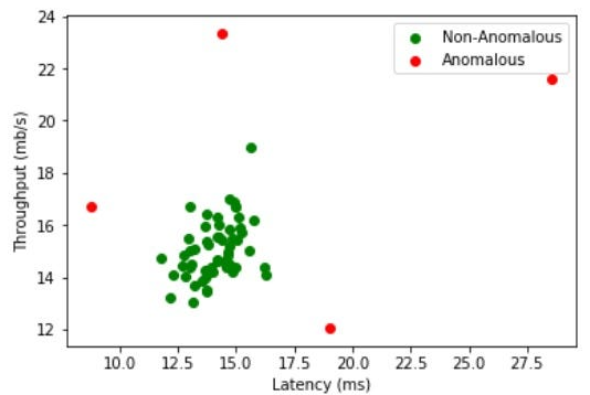
Finding Unusual Events
Anomaly detection is the process of identifying rare or unusual patterns in data that do not conform to expected behavior. These anomalies may indicate critical situations such as fraud detection, system failures, or rare events in various fields like healthcare and finance.
Real-World Examples
- Credit Card Fraud Detection: Identifying suspicious transactions that deviate significantly from a user’s normal spending habits.
- Manufacturing Defects: Detecting faulty products by identifying unusual patterns in production metrics.
- Network Intrusion Detection: Identifying cyber attacks by detecting unusual network traffic.
- Medical Diagnosis: Finding abnormal patterns in medical data that may indicate disease.
Gaussian (Normal) Distribution
The Gaussian distribution, also known as the normal distribution, is a fundamental probability distribution in statistics and machine learning. It is defined as:
Where:
- is the mean (expected value)
- is the variance
- is the variable of interest
Properties of Gaussian Distribution
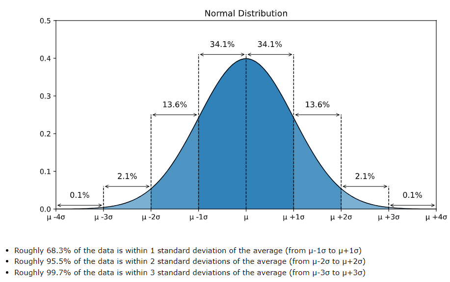
- Symmetric: Centered around the mean
- Rule:
- of values lie within standard deviation () of the mean.
- within standard deviations.
- within standard deviations.
Gaussian distribution is often used in anomaly detection to model normal behavior, where deviations from this distribution indicate anomalies.
Anomaly Detection Algorithm
Steps in Anomaly Detection
- Feature Selection: Identify relevant features from the dataset.
- Model Normal Behavior: Fit a probability distribution (e.g., Gaussian) to the normal data.
- Calculate Probability Density: Use the learned distribution to compute the probability density of new data points.
- Set a Threshold: Define a threshold below which data points are classified as anomalies.
- Detect Anomalies: Compare new observations against the threshold.
Mathematical Approach
For a feature , assuming a Gaussian distribution:
If is lower than a predefined threshold , then is considered an anomaly:
Developing and Evaluating an Anomaly Detection System
Data Preparation
- Obtain a labeled dataset with normal and anomalous instances
- Preprocess data: Handle missing values, normalize features
Model Training
- Estimate parameters and using training data:
- Compute probability density for test data
- Set anomaly threshold
Performance Evaluation
- Precision-Recall Tradeoff: Higher recall means catching more anomalies but may include false positives.
- F1 Score: Harmonic mean of precision and recall.
- ROC Curve: Evaluates different threshold settings.
5. Anomaly Detection vs. Supervised Learning
| Feature | Anomaly Detection | Supervised Learning |
|---|---|---|
| Labels Required? | No | Yes |
| Works with Unlabeled Data? | Yes | No |
| Suitable for Rare Events? | Yes | No |
| Examples | Fraud detection, Manufacturing defects | Spam detection, Image classification |
Choosing What Features to Use
- Domain Knowledge: Understand which features are relevant.
- Statistical Analysis: Use correlation matrices and distributions.
- Feature Scaling: Normalize or standardize data.
- Dimensionality Reduction: Use PCA or Autoencoders to reduce noise.
Full Python Example with TensorFlow
import numpy as np
import tensorflow as tf
from scipy.stats import norm
import matplotlib.pyplot as plt

# Generate synthetic normal data
np.random.seed(42)
data = np.random.normal(loc=50, scale=10, size=1000)

# Compute mean and variance
mu = np.mean(data)
sigma = np.std(data)

# Define probability density function
pdf = norm(mu, sigma).pdf(data)

# Set anomaly threshold (e.g., 0.001 percentile)
threshold = np.percentile(pdf, 1)

# Generate new test points
new_data = np.array([30, 50, 70, 100])
new_pdf = norm(mu, sigma).pdf(new_data)

# Detect anomalies
anomalies = new_data[new_pdf < threshold]
print("Anomalies detected:", anomalies)

# Plot
plt.figure(figsize=(10, 6))
plt.hist(data, bins=30, density=True, alpha=0.6, color='g')
x = np.linspace(min(data), max(data), 1000)
plt.plot(x, norm(mu, sigma).pdf(x), 'r', linewidth=2)
plt.scatter(anomalies, norm(mu, sigma).pdf(anomalies), color='red', marker='x', s=100, label='Anomalies')
plt.legend()
plt.show()
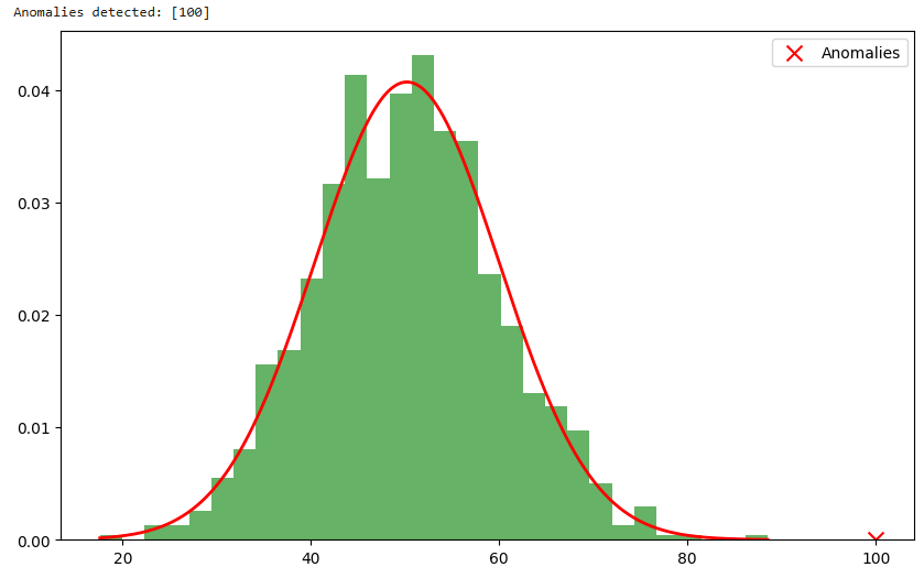
Explanation
- Generate synthetic data: We create a normal dataset.
- Compute mean and variance: Model normal behavior.
- Calculate probability density: Determine likelihood of each data point.
- Set threshold: Define an anomaly cutoff.
- Detect anomalies: Compare new observations against the threshold.
- Visualize results: Show normal distribution and detected anomalies.
This example provides a foundation for anomaly detection using probability distributions and can be extended with deep learning techniques like autoencoders or Gaussian Mixture Models (GMMs).