- Linear Regression and Cost Function
Linear Regression and Cost Function
1. Introduction
Linear regression is one of the fundamental algorithms in machine learning. It is widely used for predictive modeling, especially when the relationship between the input and output variables is assumed to be linear. The primary goal is to find the best-fitting line that minimizes the error between predicted values and actual values.
Why Linear Regression?
Linear regression is simple yet powerful for many real-world applications. Some common use cases include:
- Predicting house prices based on features like size, number of rooms, and location.
- Estimating salaries based on experience, education level, and industry.
- Understanding trends in various fields like finance, healthcare, and economics.
Real-World Example: Housing Prices
Consider predicting house prices based on the size of the house (in square meters). A simple linear relationship can be assumed: larger houses tend to have higher prices. This assumption is the foundation of our linear regression model.
2. Mathematical Representation
A simple linear regression model assumes a linear relationship between the input (house size in square meters) and the output (house price). It is represented as:
where:
- is the predicted house price.
- (intercept) and (slope) are the parameters of the model.
- is the house size.
- is the actual house price.
2.1 Understanding the Linear Model
But what does this equation really mean?
-
(intercept): The price of a house when its size is 0 m².
-
(slope): The increase in house price for every additional square meter.
For example, if:
-
and ,
-
A 100 m² house would cost:
-
A 200 m² house would cost:
We can visualize this relationship using a regression line.
3. Implementing Linear Regression Step by Step
To make the theoretical concepts clearer, let’s implement the regression model step by step using Python.
3.1 Import Necessary Libraries
import numpy as np
import matplotlib.pyplot as plt
import seaborn as sns
3.2 Generate Sample Data
np.random.seed(42)
x = 50 + 200 * np.random.rand(100, 1)  # House sizes in m² (50 to 250)
y = 50000 + 300 * x + np.random.randn(100, 1) * 5000  # House prices with noise
Here, we create a dataset with 100 samples, where:
-
represents house sizes (random values between and m²).
-
represents house prices, following a linear relation but with some noise.
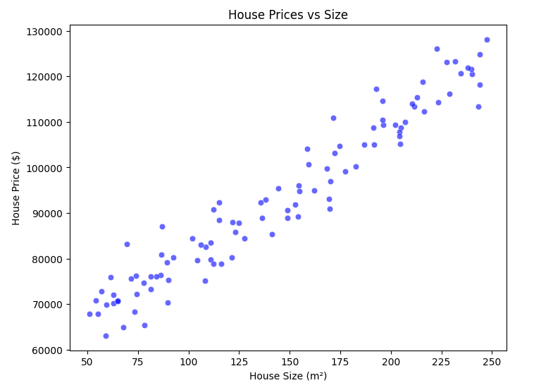
3.3 Visualizing the Data
plt.figure(figsize=(8,6))
sns.scatterplot(x=x.flatten(), y=y.flatten(), color='blue', alpha=0.6)
plt.xlabel('House Size (m²)')
plt.ylabel('House Price ($)')
plt.title('House Prices vs Size')
plt.show()
3.4 Plotting the Regression Line
Before moving to cost function, let’s fit a simple regression line to our data and visualize it.
In real-world applications, we don’t manually compute these parameters. Instead, we use libraries like scikit-learn to perform linear regression efficiently.
3.4.1 Compute the Slope ()
theta_1 = np.sum((x - np.mean(x)) * (y - np.mean(y))) / np.sum((x - np.mean(x))**2)
Here, we compute the slope () using the least squares method.
3.4.2 Compute the Intercept ()
theta_0 = np.mean(y) - theta_1 * np.mean(x)
This calculates the intercept (), ensuring that our regression line passes through the mean of the data.
3.5 Plotting the Regression Line
y_pred = theta_0 + theta_1 * x  # Compute predicted values

plt.figure(figsize=(8,6))
sns.scatterplot(x=x.flatten(), y=y.flatten(), color='blue', alpha=0.6, label='Actual Data')
plt.plot(x, y_pred, color='red', linewidth=2, label='Regression Line')
plt.xlabel('House Size (m²)')
plt.ylabel('House Price ($)')
plt.title('Linear Regression Model: House Prices vs. Size')
plt.legend()
plt.show()
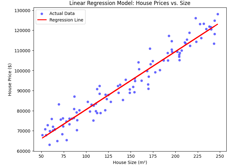
3.6 Interpretation of the Regression Line
Now, what does this line tell us?
✅ If the slope is positive, then larger houses cost more (as expected).
✅ If the intercept is high, it means even the smallest houses have a significant base price.
✅ The steepness of the line shows how much price increases per square meter.
4. Cost Function
To measure how well our model is performing, we use the cost function. The most common cost function for linear regression is the Mean Squared Error (MSE):
where:
- is the number of training examples.
- is the predicted price for the house.
- is the actual price.
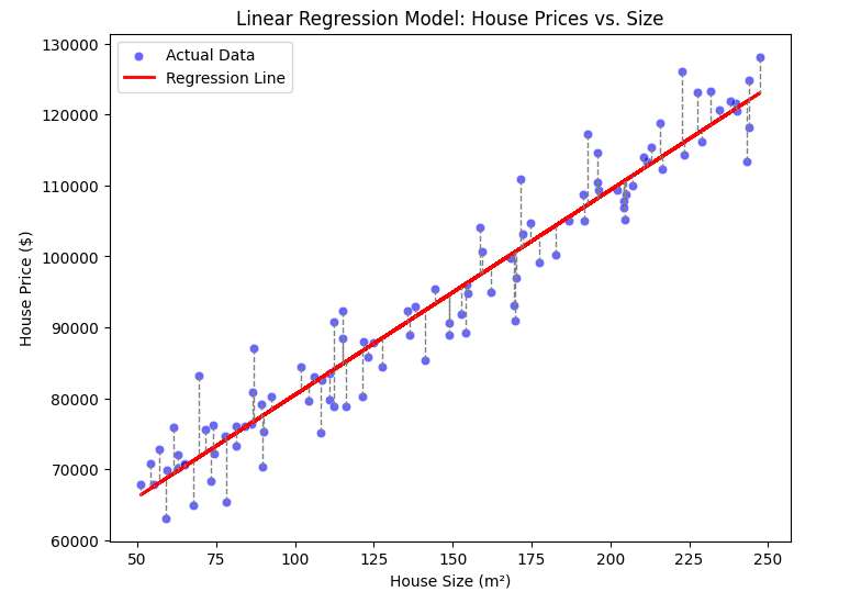
Any dashed line indicates an error. In the formula above, we calculated the sum of these, namely .
This function calculates the average squared difference between predicted and actual values, penalizing larger errors more. The goal is to minimize to achieve the best model parameters.
4.1 Example: Assuming
To illustrate how the cost function behaves, let’s assume that , meaning our model only depends on . We’ll use a small dataset with four x values and y values:
| x values | y values |
|---|---|
| 1 | 2 |
| 2 | 4 |
| 3 | 6 |
| 4 | 8 |
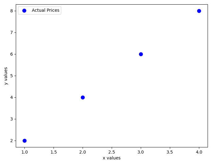
Since we assume , our hypothesis function simplifies to:
We’ll evaluate different values of and compute the corresponding cost function.
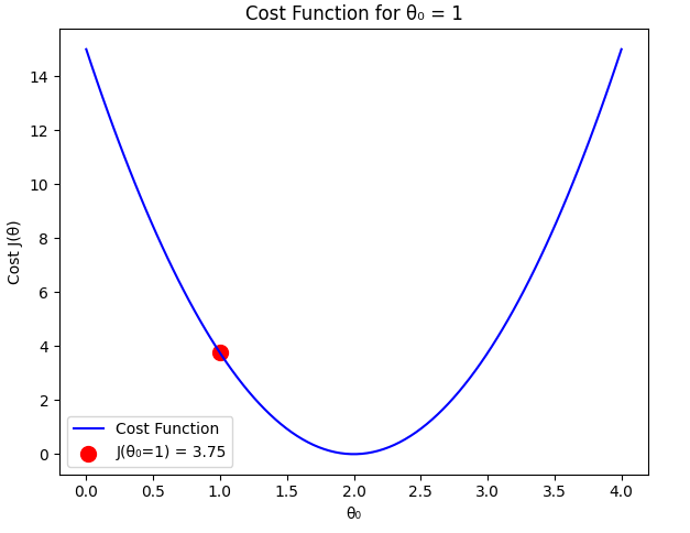
Case 1:
For , the predicted values are:
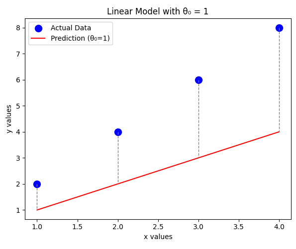
The error values:
Computing the cost function:
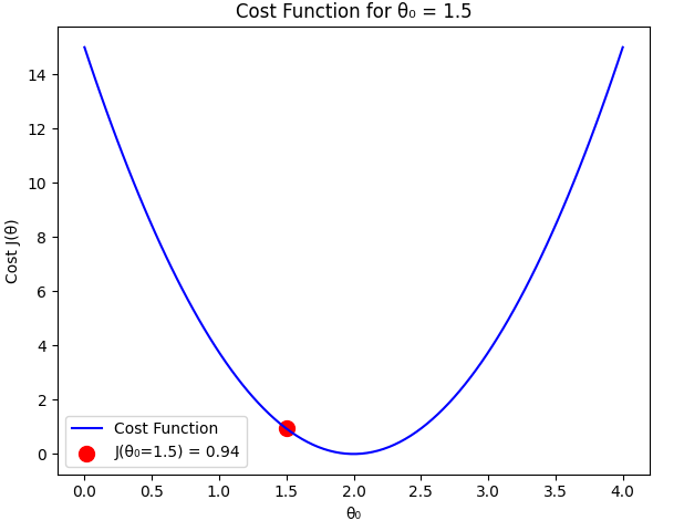
Case 2:
For , the predicted values are:
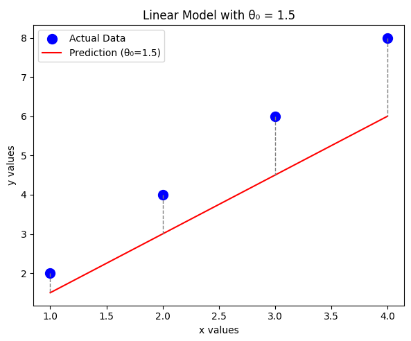
The error values:
Computing the cost function:
Case 3: (Optimal Case)
For , the predicted values match the actual values:
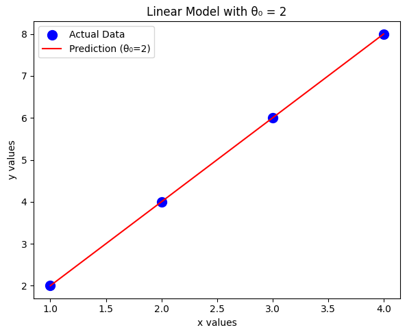
The error values:
Computing the cost function:
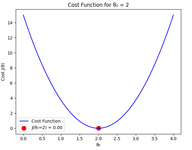
Comparison
From our calculations:
As expected, the cost function is minimized when , which perfectly fits the dataset. Any deviation from this value results in a higher cost.
So how many times can the machine try and find the correct value? How can we teach it this? The answer is in the next topic.