ai

• Introduction to Gradient Descent
• Mathematical Formulation of Gradient Descent
  • 1. Gradient Descent Update Rule
    • Why Do We Use the Derivative?
  • 2. Computing the Gradient
• Learning Rate ($\alpha$)
  • 1. When $\alpha$ is Too Small
  • 2. When $\alpha$ is Optimal
  • 3. When $\alpha$ is Too Large
  • Summary
• Gradient Descent Convergence
  • 1. Convergence Criteria
  • 2. Choosing the Right Stopping Condition
• Local Minimum vs Global Minimum
  • Understanding the Concept
  • Convex vs Non-Convex Cost Functions

Introduction to Gradient Descent

In the previous section, we explored how the cost function behaves when assuming different values of ${\theta }_0$ with ${\theta }_1=0$ (To visualize it easily, we give zero to ${\theta }_1$). Now, we introduce Gradient Descent, an optimization algorithm used to find the best parameters that minimize the cost function $J(\theta )$.

our hypothesis function simplifies to: $$h_{\theta }(x)={\theta }_0\cdot x$$

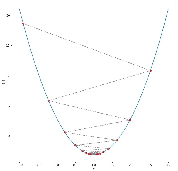
Gradient Descent is an iterative method that updates the parameter $\theta$ step by step in the direction that reduces the cost function. The algorithm helps us find the optimal value of ${\theta }_0$ efficiently instead of manually testing different values.

To understand how Gradient Descent works, let's recall our dataset:

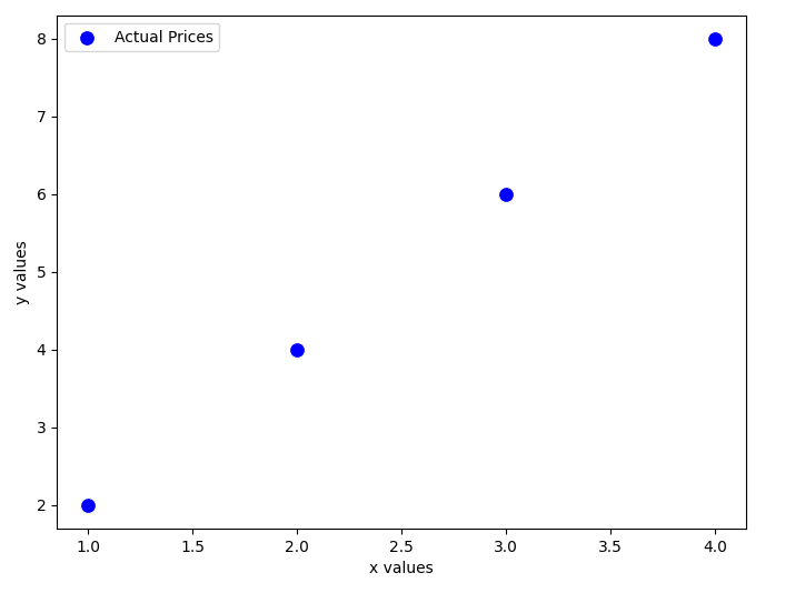
We aim to find the best value of ${\theta }_0$ that minimizes the error between our predictions $h_{\theta }(x)={\theta }_0\cdot x$ and the actual $y$ values. Gradient Descent will iteratively adjust ${\theta }_0$ to reach the minimum cost.

Mathematical Formulation of Gradient Descent

Gradient Descent is an optimization algorithm used to minimize a function by iteratively updating its parameters in the direction of the steepest descent. In our case, we aim to minimize the cost function:

$$J(\theta )=\frac{1}{2m}\sum (h_{\theta }(x_i)-y_i{)}^2$$

Where:

• 𝑚 is the number of training examples.
• $h_{\theta }(x)$ represents our hypothesis function (predicted values).
• y represents the actual target values.
• Goal: Find the optimal $\theta$ that minimizes $J(\theta )$.

1. Gradient Descent Update Rule

Gradient Descent uses the derivative of the cost function to determine the direction and magnitude of updates. The general update rule for $\theta$ is:

$$\theta :=\theta -\alpha \frac{\partial J(\theta )}{\partial \theta }$$

Where:

• $\alpha$ (learning rate) controls the step size of updates.
• $\frac{\partial J(\theta )}{\partial \theta }$ is the gradient (derivative) of the cost function with respect to $\theta$.

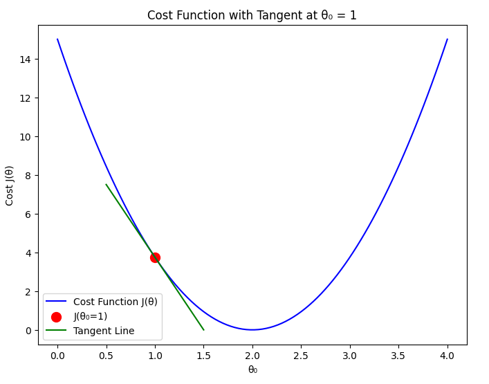
Why Do We Use the Derivative?

The derivative $\frac{\partial J(\theta )}{\partial \theta }$ tells us the slope of the cost function. If the slope is positive, we need to decrease ${\theta }_0$ , and if it is negative, we need to increase ${\theta }_0$, guiding us toward the minimum of $J({\theta }_0)$ . Without derivatives, we wouldn't know which direction to move to minimize the function.

The gradient tells us how steeply the function increases or decreases at a given point.

• If the gradient is positive, $\theta$ is decreased.
• If the gradient is negative, $\theta$ is increased.

This ensures that we move toward the minimum of the cost function.

2. Computing the Gradient

First, recall our hypothesis function:

$$h_{\theta }(x)={\theta }_0\cdot x$$

Now, we compute the derivative of the cost function:

$$\frac{\partial J(\theta )}{\partial \theta \ast 0}=\frac{1}{m}\sum (h_{\theta }(x^{(i)})-y^{(i)})x^{(i)}$$

This expression represents the average gradient of the errors multiplied by the input values. Using this gradient, we update ${\theta }_0$ in each iteration:

$$\theta \ast 0:={\theta }_0-\alpha \cdot \frac{1}{m}\sum (h_{\theta }(x^{(i)})-y^{(i)})x^{(i)}$$

• If the error is large, the update step is bigger.
• If the error is small, the update step is smaller.

This way, the algorithm gradually moves towards the optimal ${\theta }_0$.

Learning Rate ($\alpha$)

The learning rate $(\alpha )$ is a crucial parameter in the gradient descent algorithm. It determines how large a step we take in the direction of the negative gradient during each iteration. Choosing an appropriate learning rate is essential for ensuring efficient convergence of the algorithm.

If the learning rate is too small, the algorithm will take tiny steps towards the minimum, leading to slow convergence. On the other hand, if the learning rate is too large, the algorithm may overshoot the minimum or even diverge, never reaching an optimal solution.

1. When $\alpha$ is Too Small

If the learning rate is set too small:

• Gradient descent will take very small steps in each iteration.
• Convergence to the minimum cost will be extremely slow.
• It may take a large number of iterations to reach a useful solution.
• The algorithm might get stuck in local variations of the cost function, slowing down learning.

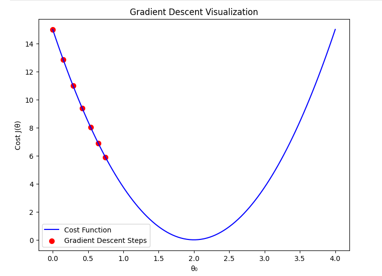
Mathematically, the update rule is: ${\theta }_0:={\theta }_0-\alpha \frac{d}{d{\theta }_0}J({\theta }_0)$ When $\alpha$ is very small, the change in ${\theta }_0$ per step is minimal, making the process inefficient.

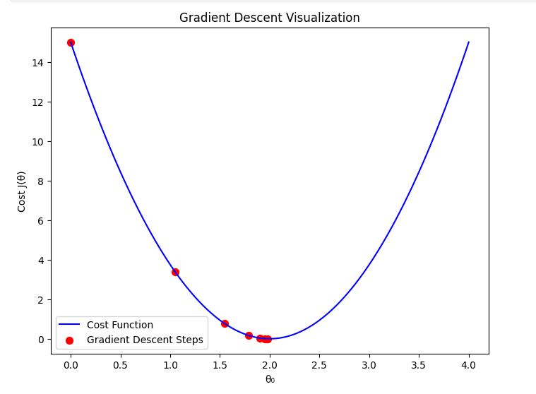
2. When $\alpha$ is Optimal

If the learning rate is chosen optimally:

• The gradient descent algorithm moves efficiently towards the minimum.
• It balances speed and stability, converging in a reasonable number of iterations.
• The cost function decreases steadily without oscillations or divergence.

A well-chosen $\alpha$ ensures that gradient descent follows a smooth and steady path to the minimum.

3. When $\alpha$ is Too Large

If the learning rate is set too large:

• Gradient descent may take excessively large steps.
• Instead of converging, it may oscillate around the minimum or diverge entirely.
• The cost function might increase instead of decreasing due to overshooting the optimal ${\theta }_0$.

In extreme cases, the cost function values might increase indefinitely, causing the algorithm to fail to find a minimum.

Summary

Selecting the right learning rate is essential for gradient descent to work efficiently. A well-balanced $\alpha$ ensures that the algorithm converges quickly and effectively. In the next section, we will implement gradient descent with different learning rates to visualize their effects.

Gradient Descent Convergence

Gradient Descent is an iterative optimization algorithm that minimizes the cost function, J(\theta), by updating parameters step by step. However, we need a proper stopping criterion to determine when the algorithm has converged.

1. Convergence Criteria

The algorithm should stop when one of the following conditions is met:

• Small Gradient: If the derivative (gradient) of the cost function is close to zero, meaning the algorithm is near the optimal point.
• Minimal Cost Change: If the difference in the cost function between iterations is below a predefined threshold ($|J(\theta \ast t)-J(\theta \ast t-1)|<\epsilon$).
• Maximum Iterations: A fixed number of iterations is reached to avoid infinite loops.

2. Choosing the Right Stopping Condition

• Stopping Too Early: If the algorithm stops before reaching the optimal solution, the model may not perform well.
• Stopping Too Late: Running too many iterations may waste computational resources without significant improvement.
• Optimal Stopping: The best condition is when further updates do not significantly change the cost function or parameters.

Local Minimum vs Global Minimum

Understanding the Concept

When optimizing a function, we aim to find the point where the function reaches its lowest value. This is crucial in machine learning because we want to minimize the cost function $J(\theta )$ effectively. However, there are two types of minima that gradient descent might encounter:

• Global Minimum: The absolute lowest point of the function. Ideally, gradient descent should converge here.
• Local Minimum: A point where the function has a lower value than nearby points but is not the absolute lowest value.

For convex functions (such as our quadratic cost function), gradient descent is guaranteed to reach the global minimum. However, for non-convex functions, the algorithm may get stuck in a local minimum.

Convex vs Non-Convex Cost Functions

1. Convex Functions

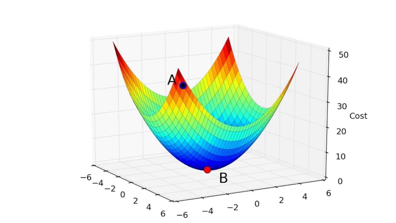
• The cost function $J(\theta )$ is convex for linear regression.
• This ensures that gradient descent always leads to the global minimum.
• Example: A simple quadratic function like $J(\theta )=(\theta -2{)}^2$.

2. Non-Convex Functions

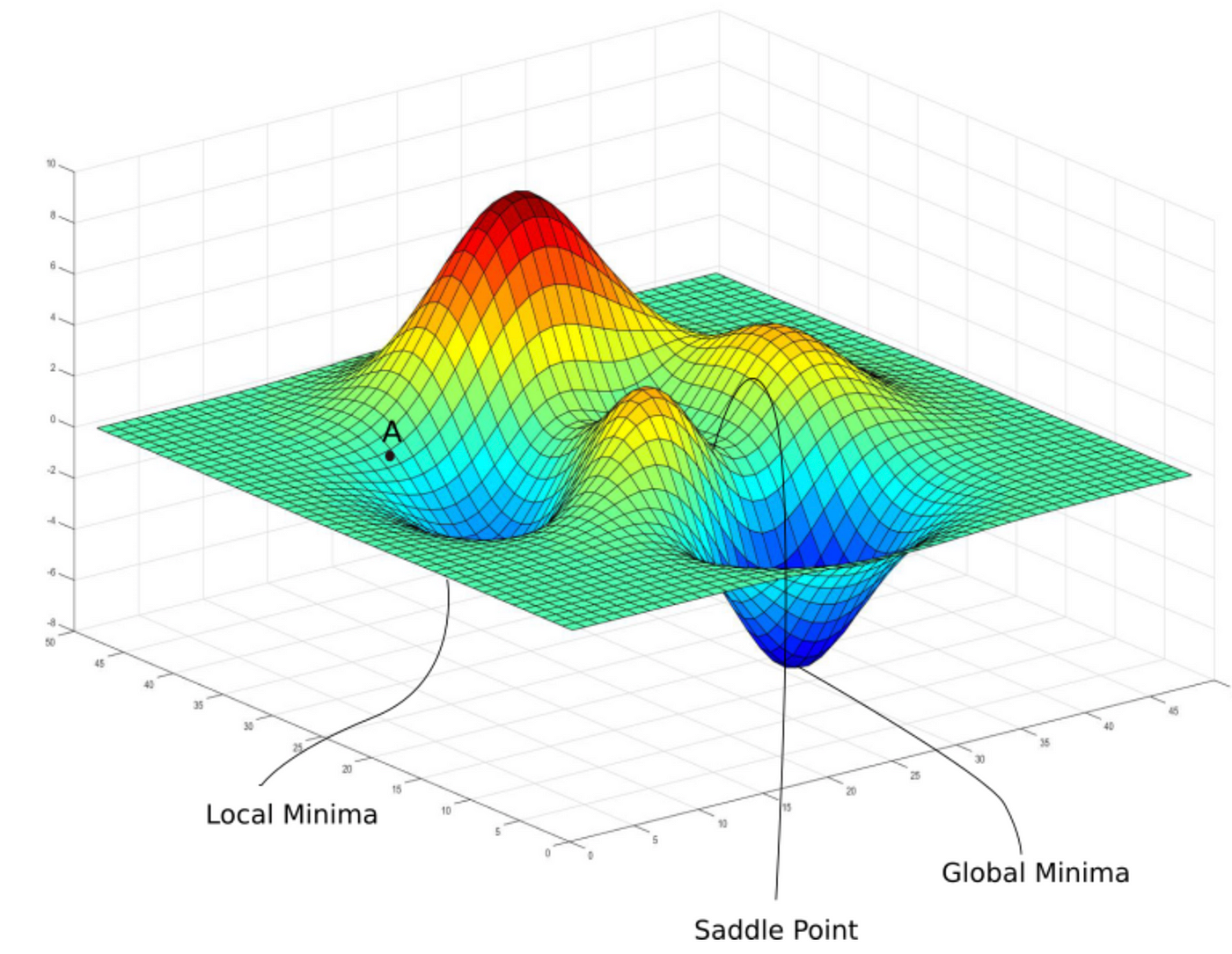
• More common in deep learning and complex machine learning models.
• There can be multiple local minima.
• Example: Functions with multiple peaks and valleys, such as $J(\theta )=\sin (\theta )+\frac{{\theta }^2}{10}$.