Feature Engineering and Polynomial Regression

• Feature Engineering
  • Introduction to Feature Engineering
    • Why is Feature Engineering Important?
    • Real-World Example
  • Feature Transformation
    • 1. Log Transformation
      • Example: Income Data
    • 2. Polynomial Features
      • Example: House Price Prediction
    • 3. Interaction Features
      • Example: Combining Features
  • Feature Selection
    • 1. Unnecessary Features
    • 2. Correlation Analysis
      • Example: Finding Highly Correlated Features
    • 3. Statistical Feature Selection Methods
      • Common Methods:
• Polynomial Regression
  • Introduction to Polynomial Regression
    • Why Use Polynomial Regression?
    • Example: Predicting House Prices
  • Mathematical Representation and Implementation

Feature Engineering

Introduction to Feature Engineering

Feature engineering is the process of transforming raw data into meaningful features that improve the predictive power of machine learning models. It involves creating new features, modifying existing ones, and selecting the most relevant features to enhance model performance.

Why is Feature Engineering Important?

• Improves model accuracy: Well-engineered features help models learn better representations of the data.
• Reduces model complexity: Properly engineered features can make complex models simpler and more interpretable.
• Enhances generalization: Good feature selection prevents overfitting and improves performance on unseen data.

Real-World Example

Consider a house price prediction problem. Instead of using just raw data such as square footage and the number of bedrooms, we can create new features like:

• Price per square foot = Price / Size
• Age of the house = Current Year - Year Built
• Proximity to city center = Distance in km

These engineered features often provide better insights and improve model performance compared to using raw data alone.

Feature Transformation

Feature transformation involves applying mathematical operations to existing features to make data more suitable for machine learning models.

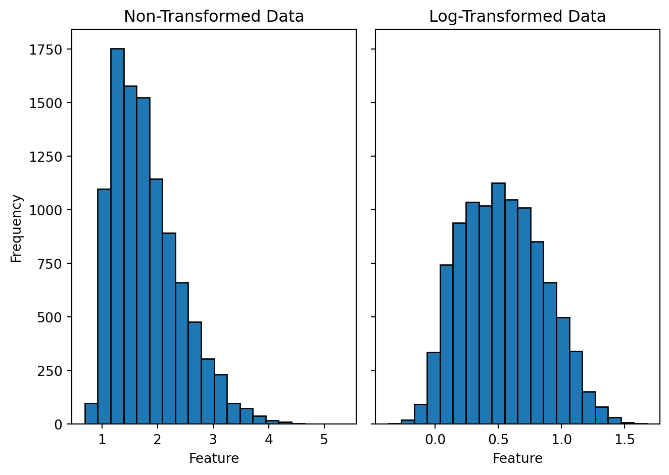
1. Log Transformation

Used to reduce skewness and stabilize variance in highly skewed data.

Example: Income Data

Many income datasets have a right-skewed distribution where most values are low, but a few values are extremely high. Applying a log transformation makes the data more normal:

$$X^{\prime }=\log (X)$$

2. Polynomial Features

Adding polynomial terms (squared, cubic) to capture non-linear relationships.

Example: House Price Prediction

Instead of using Size as a single feature, we can include Size^2 and Size^3 to better fit non-linear patterns.

from sklearn.preprocessing import PolynomialFeatures
import numpy as np

X = np.array([[1000], [1500], [2000], [2500]])  # House sizes
poly = PolynomialFeatures(degree=2)
X_poly = poly.fit_transform(X)
print(X_poly)

3. Interaction Features

Creating new features based on interactions between existing ones.

Example: Combining Features

Instead of using Height and Weight separately for a health model, create a new BMI feature:

$$BMI=\frac{Weight}{Heigh{t}^2}$$

def calculate_bmi(height, weight):
    return weight / (height ** 2)

height = np.array([1.65, 1.75, 1.80])  # Heights in meters
weight = np.array([65, 80, 90])  # Weights in kg
bmi = calculate_bmi(height, weight)
print(bmi)

This allows the model to understand health risks better than using height and weight separately.

Feature Selection

Feature selection involves identifying the most relevant features for a model while removing unnecessary or redundant ones. This improves model performance and reduces computational complexity.

1. Unnecessary Features

Not all features contribute equally to model performance. Some may be irrelevant or redundant, leading to overfitting and increased computational cost. Examples of unnecessary features include:

• ID columns: Unique identifiers that do not provide predictive value.
• Highly correlated features: Features that contain similar information.
• Constant or near-constant features: Features with little to no variation.

2. Correlation Analysis

Correlation analysis helps detect multicollinearity, where two or more features are highly correlated. If two features provide similar information, one of them can be removed.

Example: Finding Highly Correlated Features

import pandas as pd
import numpy as np

# Sample dataset
data = {
    'Feature1': [1, 2, 3, 4, 5],
    'Feature2': [2, 4, 6, 8, 10],
    'Feature3': [5, 3, 6, 9, 2]
}
df = pd.DataFrame(data)

# Compute correlation matrix
correlation_matrix = df.corr()
print(correlation_matrix)

Features with a correlation coefficient close to ±1 can be considered redundant and removed.

3. Statistical Feature Selection Methods

Feature selection techniques can be used to rank the importance of different features based on statistical tests or model-based importance measures.

At this stage it is enough to learn superficially !

Common Methods:

• Chi-Square Test: Measures dependency between categorical features and the target variable.
• Mutual Information: Evaluates how much information a feature contributes.
• Recursive Feature Elimination (RFE): Iteratively removes less important features based on model performance.
• Feature Importance from Tree-Based Models: Decision trees and random forests provide feature importance scores.

Feature selection ensures that only the most valuable features are used in the final model, improving efficiency and predictive power.

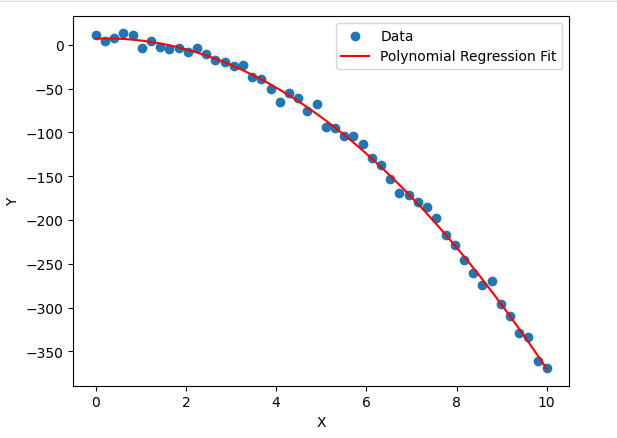
Polynomial Regression

Introduction to Polynomial Regression

Polynomial Regression is an extension of Linear Regression that models non-linear relationships between input features and the target variable. While Linear Regression assumes a straight-line relationship, Polynomial Regression captures curves and more complex patterns.

Why Use Polynomial Regression?

• Handles Non-Linearity: Unlike Linear Regression, which assumes a direct relationship, Polynomial Regression models curved trends.
• Better Fit for Real-World Data: Many real-world phenomena, such as population growth, economic trends, and physics-based models, exhibit non-linear behavior.
• Feature Engineering Alternative: Instead of manually creating interaction terms, Polynomial Regression provides an automatic way to capture complex dependencies.

Example: Predicting House Prices

Consider a dataset where house prices do not increase linearly with size. Instead, they follow a non-linear trend due to factors like demand, location, and infrastructure. A Polynomial Regression model can better capture this pattern.

For instance:

• Linear Model: $Price={\beta }_0+{\beta }_1\cdot Size$
• Polynomial Model: $Price={\beta }_0+{\beta }_1\cdot Size+{\beta }_2\cdot Siz{e}^2$

This quadratic term helps model the curved price trend more accurately.

Mathematical Representation and Implementation

Polynomial regression extends linear regression by adding polynomial terms to the feature set. The hypothesis function is represented as:

$$h_{\theta }(x)={\theta }_0+{\theta }_{1}x+{\theta }_2{x}^2+{\theta }_3{x}^3+...+{\theta }_n{x}^n$$

where:

• $x$ is the input feature,
• ${\theta }_0,{\theta }_1,...,{\theta }_n$ are the parameters (weights),
• $x^n$ represents higher-degree polynomial terms.

This allows the model to capture non-linear relationships in the data.