Classification with Logistic Regression
- 1. Introduction to Classification
- 2. Logistic Regression
- 3. Cost Function for Logistic Regression
- 4. Gradient Descent for Logistic Regression
1. Introduction to Classification
Classification is a supervised learning problem where the goal is to predict discrete categories instead of continuous values. Unlike regression, which predicts numerical values, classification assigns data points to labels or classes.
Classification vs. Regression
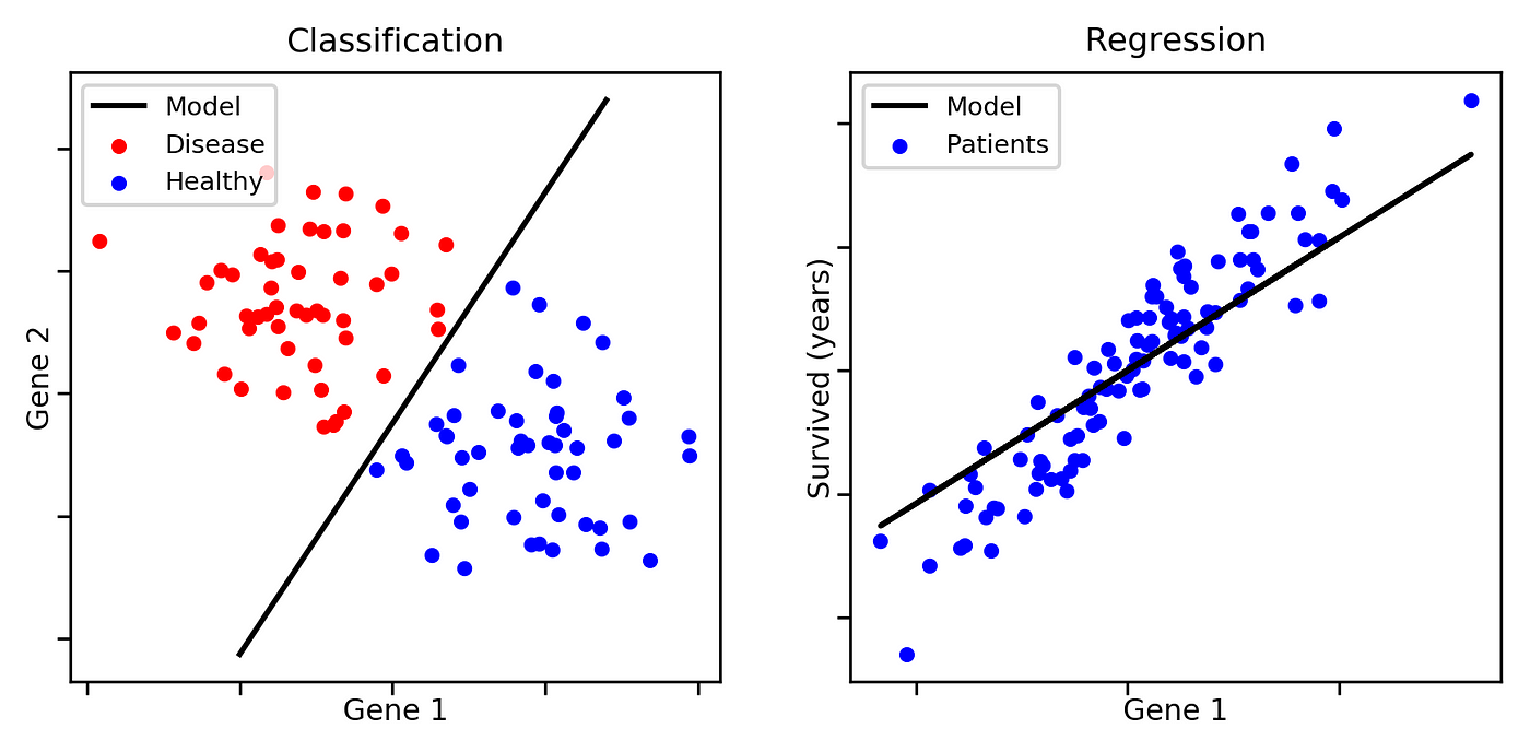
| Feature | Regression | Classification |
|---|---|---|
| Output Type | Continuous | Discrete |
| Example | Predicting house prices | Email spam detection |
| Algorithm Example | Linear Regression | Logistic Regression |
Examples of Classification Problems
- Email Spam Detection: Classify emails as “spam” or “not spam”.
- Medical Diagnosis: Identify whether a patient has a disease (yes/no).
- Credit Card Fraud Detection: Determine if a transaction is fraudulent or legitimate.
- Image Recognition: Classifying images as “cat” or “dog”.
Classification models can be:
- Binary Classification: Only two possible outcomes (e.g., spam or not spam).
- Multi-class Classification: More than two possible outcomes (e.g., classifying handwritten digits 0-9).
2. Logistic Regression
Introduction to Logistic Regression
Logistic regression is a statistical model used for binary classification problems. Unlike linear regression, which predicts continuous values, logistic regression predicts probabilities that map to discrete class labels.
Linear regression might seem like a reasonable approach for classification, but it has major limitations:
- Unbounded Output: Linear regression produces outputs that can take any real value, meaning predictions could be negative or greater than 1, which makes no sense for probability-based classification.
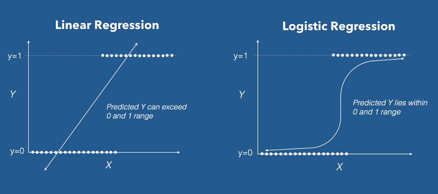
- Poor Decision Boundaries: If we use a linear function for classification, extreme values in the dataset can distort the decision boundary, leading to incorrect classifications.
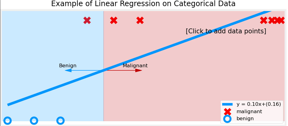
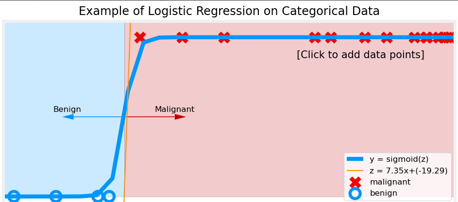
To solve these issues, we use logistic regression, which applies the sigmoid function to transform outputs into a probability range between 0 and 1.
Why Do We Need the Sigmoid Function?
The sigmoid function is a key component of logistic regression. It ensures that outputs always remain between 0 and 1, making them interpretable as probabilities.
Consider a fraud detection system that predicts whether a transaction is fraudulent (1) or legitimate (0) based on customer behavior. Suppose we use a linear model:
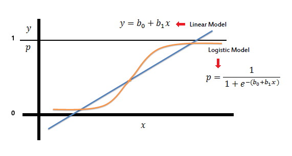
For some transactions, the output might be y = 7.5 or y = -3.2, which do not make sense as probability values. Instead, we use the sigmoid function to squash any real number into a valid probability range:
This function maps:
- Large positive values to probabilities close to 1 (fraudulent transaction).
- Large negative values to probabilities close to 0 (legitimate transaction).
- Values near 0 to probabilities near 0.5 (uncertain classification).
Sigmoid Function and Probability Interpretation
The output of the sigmoid function can be interpreted as:
- → The model predicts Class 1 (e.g., spam email, fraudulent transaction).
- → The model predicts Class 0 (e.g., not spam email, legitimate transaction).
For a final classification decision, we apply a threshold (typically 0.5):
This means:
- If the probability is ≥ 0.5, we classify the input as 1 (positive class).
- If the probability is < 0.5, we classify it as 0 (negative class).
Decision Boundary
The decision boundary is the surface that separates different classes in logistic regression. It is the point at which the model predicts a probability of 0.5, meaning the model is equally uncertain about the classification.
Since logistic regression produces probabilities using the sigmoid function, we define the decision boundary mathematically as:
Taking the inverse of the sigmoid function, we get:
This equation defines the decision boundary as a linear function in the feature space.
Understanding the Decision Boundary with Examples
1. Single Feature Case (1D)
If we have only one feature , the model equation is:
Solving for :
This means that when crosses this threshold, the model switches from predicting Class 0 to Class 1.
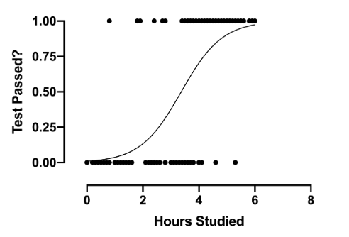
Example: Imagine predicting whether a student passes or fails based on study hours ():
- If hours → Fail (Class 0).
- If hours → Pass (Class 1).
The decision boundary in this case is simply .
2. Two Features Case (2D)
For two features and , the decision boundary equation becomes:
Rearranging:
This represents a straight line separating the two classes in a 2D plane.
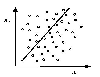
Example: Suppose we classify students as passing (1) or failing (0) based on study hours () and sleep hours ():
- The decision boundary could be:
- If is above the line, classify as pass.
- If is below the line, classify as fail.
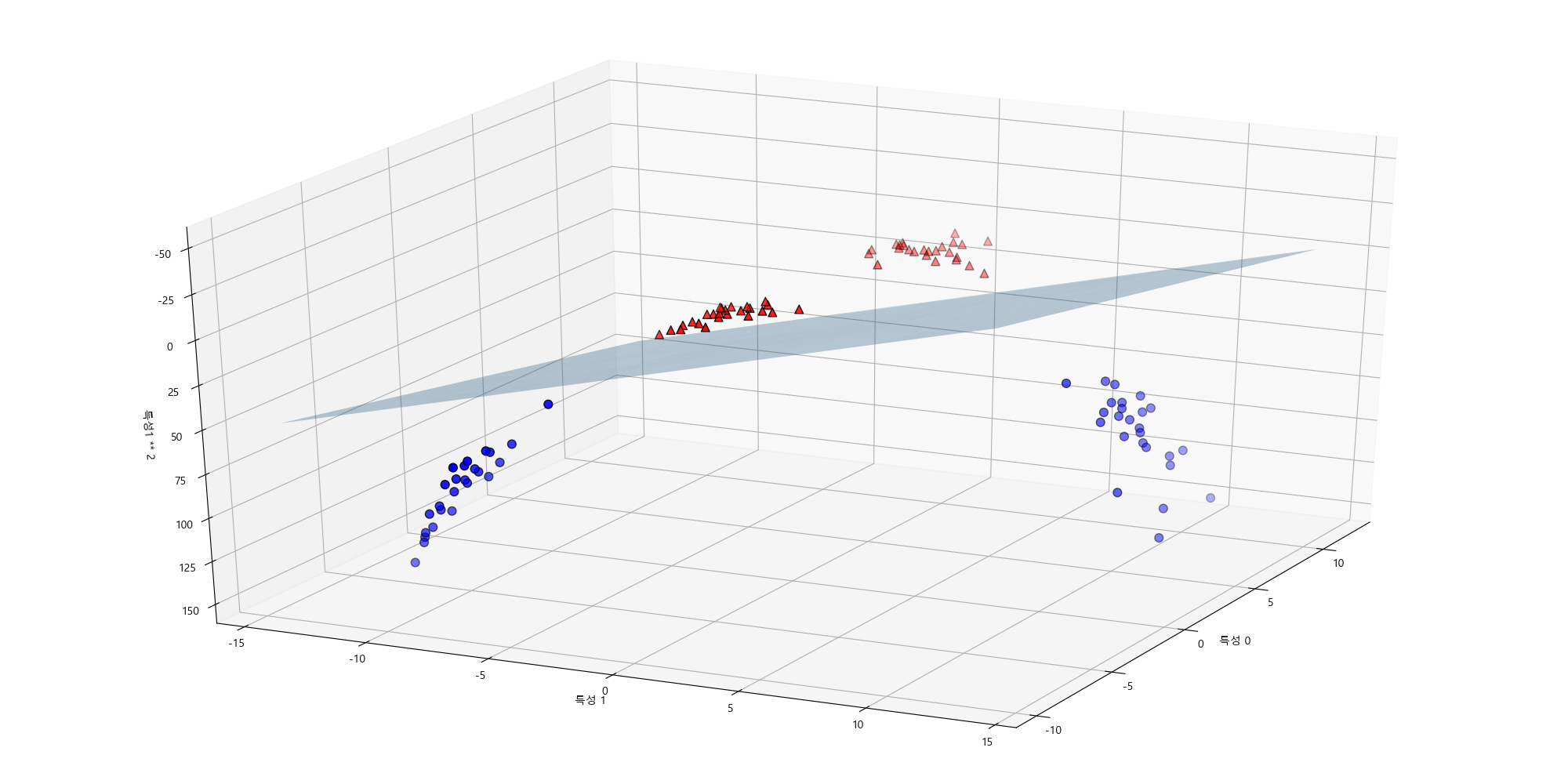
3. Two Features Case (3D)
When we move to three features , , and , the decision boundary becomes a plane in three-dimensional space:
Rearranging for :
This equation represents a flat plane dividing the 3D space into two regions, one for Class 1 and the other for Class 0.
Example:
Imagine predicting whether a company will be profitable (1) or not (0) based on:
- Marketing Budget ()
- R&D Investment ()
- Number of Employees ()
The decision boundary would be a plane in 3D space, separating profitable and non-profitable companies.
In general, for n features, the decision boundary is a hyperplane in an n-dimensional space.
4. Non-Linear Decision Boundaries in Depth
So far, we have seen that logistic regression creates linear decision boundaries. However, many real-world problems have non-linear relationships. In such cases, a straight line (or plane) is not sufficient to separate classes.
To capture complex decision boundaries, we introduce polynomial features or feature transformations.
Example 1: Circular Decision Boundary
If the data requires a circular boundary, we can use quadratic terms:
This represents a circle in 2D space.
For example:
-
If and are the coordinates of points, a decision boundary like:
would classify points inside a radius-2 circle as Class 1 and outside as Class 0.
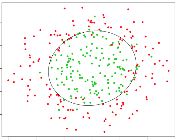
Example 2: Elliptical Decision Boundary
A more general quadratic equation:
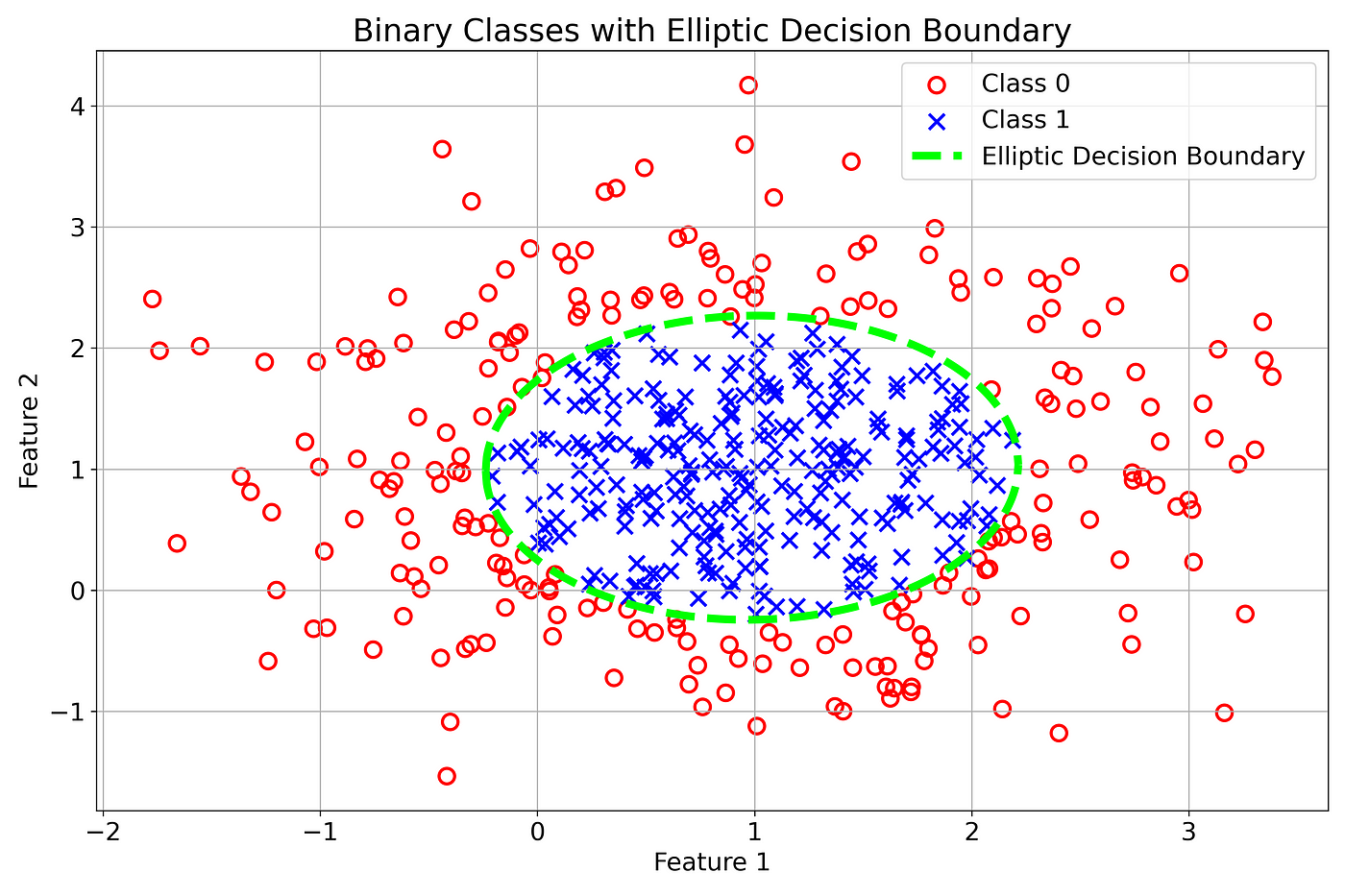
This allows for elliptical decision boundaries.
Example 3: Complex Non-Linear Boundaries
For even more complex boundaries, we can include higher-order polynomial features, such as:
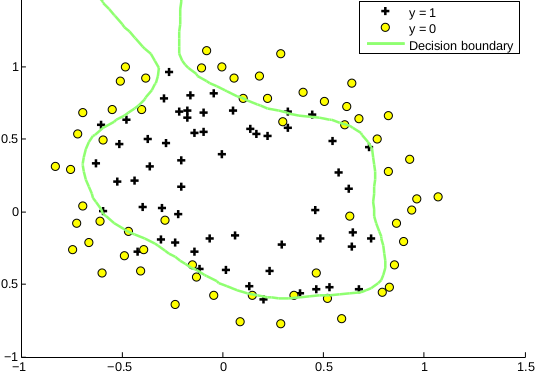
This enables twists and curves in the decision boundary, allowing logistic regression to model highly non-linear patterns.
Feature Engineering for Non-Linear Boundaries
- Instead of adding polynomial terms manually, we can transform features using basis functions (e.g., Gaussian kernels or radial basis functions).
- Feature maps can convert non-linearly separable data into a higher-dimensional space where a linear decision boundary works.
Limitations of Logistic Regression for Non-Linear Boundaries
- Feature engineering is required: Unlike neural networks or decision trees, logistic regression cannot learn complex boundaries automatically.
- Higher-degree polynomials can lead to overfitting: Too many non-linear terms make the model sensitive to noise.
Key Takeaways
- In 3D, the decision boundary is a plane, and in higher dimensions, it becomes a hyperplane.
- Non-linear decision boundaries can be created using quadratic, cubic, or transformed features.
- Feature engineering is crucial to make logistic regression work well for non-linearly separable problems.
- Too many high-order polynomial terms can cause overfitting, so regularization is needed.
3. Cost Function for Logistic Regression
1. Why Do We Need a Cost Function?
In linear regression, we use the Mean Squared Error (MSE) as the cost function:
However, this cost function does not work well for logistic regression because:
- The hypothesis function in logistic regression is non-linear due to the sigmoid function.
- Using squared errors results in a non-convex function with multiple local minima, making optimization difficult.
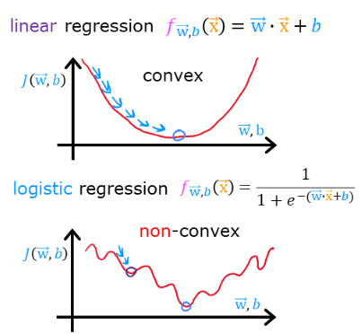
We need a different cost function that:
✅ Works well with the sigmoid function.
✅ Is convex, so gradient descent can efficiently minimize it.
2. Simplified Cost Function for Logistic Regression
Instead of using squared errors, we use a log loss function:
Where:
- is the true label (0 or 1).
- is the predicted probability from the sigmoid function.
This function ensures:
- If → The first term dominates: , which is close to 0 if (correct prediction).
- If → The second term dominates: , which is close to 0 if .
✅ Interpretation: The function penalizes incorrect predictions heavily while rewarding correct predictions.
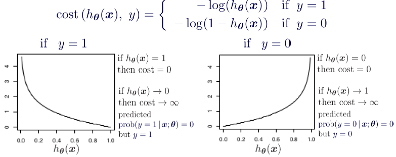
3. Intuition Behind the Cost Function
Let’s break it down:
-
When , the cost function simplifies to:
This means:
- If (correct prediction), → No penalty.
- If (wrong prediction), → High penalty!
-
When , the cost function simplifies to:
This means:
- If (correct prediction), → No penalty.
- If (wrong prediction), → High penalty!
✅ Key Takeaway:
The function assigns very high penalties for incorrect predictions, encouraging the model to learn correct classifications.
4. Gradient Descent for Logistic Regression
1. Why Do We Need Gradient Descent?
In logistic regression, our goal is to find the best parameters that minimize the cost function:
Since there is no closed-form solution like in linear regression, we use gradient descent to iteratively update until we reach the minimum cost.
2. Gradient Descent Algorithm
Gradient descent updates the parameters using the rule:
Where:
- is the learning rate (step size).
- is the gradient (direction of steepest increase).
For logistic regression, the derivative of the cost function is:
Thus, the update rule becomes:
✅ Key Insight:
- We compute the error: .
- Multiply it by the feature .
- Average over all training examples.
- Scale by and update .