Using Segmentation to Find Suspected Nodules
- 1. The Cancer Detection Pipeline: Why Candidate Proposal is Essential
- 2. Section 2.7 System Roadmap
- 3. Classification vs. Semantic Segmentation: The Per-Pixel Spatial Mandate
- 4. Foundation Models in Vision: Meta’s Segment Anything Model (SAM)
- 5. Volumetric Slicing: Bridging 3D CT Scans to 2D Foundation Models
- 6. Building the Segmentation Dataset with SAM Pseudo-Ground-Truth
- 7. Fully Automated Unprompted Segmentation with SegFormer
- 8. Loss Functions for Extreme Foreground-Background Imbalance: BCE + Dice Loss
- 9. Training, Checkpointing, and Candidate Coordinate Extraction
- 10. Summary and Key Insights

1. The Cancer Detection Pipeline: Why Candidate Proposal is Essential
In Sections 2.5 and 2.6, we designed, trained, and optimized a 3D Convolutional Neural Network (LunaModel) capable of discriminating small volumetric crops into malignant tumors versus benign anatomical structures. Through precision-recall metrics and 3D affine data augmentations, we achieved an effective clinical classifier.
However, that classifier operated under a massive foundational assumption: it required candidate coordinate locations to be provided beforehand. In the LUNA dataset, candidate locations were provided by expert radiologist annotations (annotations.csv and candidates.csv).
In a genuine hospital radiology environment, when a patient undergoes a low-dose computed tomography (CT) scan, the system is handed raw volumetric data with zero annotations. A standard CT scan encompasses a volume of approximately $512 \times 512 \times 400$ voxels—roughly 100 million voxels. If we were to slide our Section 2.5 3D classifier across every possible $32 \times 48 \times 48$ subvolume in the chest cavity, we would evaluate tens of millions of windows. This brute-force sliding-window approach suffers from two fatal flaws:
- Extreme Computational Latency: Evaluating millions of 3D convolutional forward passes per patient would require tens of minutes of GPU compute per scan.
- False Positive Explosion: Even with a 99.9% specificity rate, evaluating $10^7$ negative windows would produce $10{,}000$ false alarms per patient, completely overwhelming radiologists.
To build an autonomous clinical screening pipeline, we need an upstream model whose purpose is candidate proposal: scanning the entire volume rapidly to flag a small handful (e.g., 20–50) of high-suspicion regions. This is the domain of Semantic Segmentation.
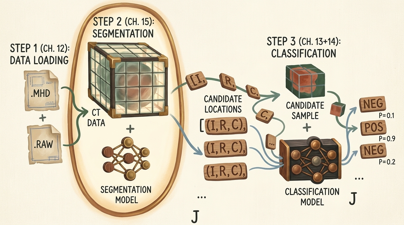
flowchart TD
    subgraph Pipeline ["Autonomous Lung Cancer Detection Pipeline"]
        direction TB
        S1["Step 1: Volumetric Data Ingestion (Section 2.4)<br/>Raw .mhd/.raw to Calibrated Hounsfield Tensors"]
        S2["Step 2: Candidate Nodule Segmentation (Section 2.7)<br/>Full-Scan Per-Pixel Proposal Model"]
        S3["Step 3: False-Positive Reduction (Sections 2.5 & 2.6)<br/>3D CNN Binary Classifier"]
        S1 --> S2 --> S3
    end

    style Pipeline fill:#1a1a2e,stroke:#4cc9f0,stroke-width:2px,color:#fff
    style S1 fill:#16213e,stroke:#4cc9f0,stroke-width:1px,color:#fff
    style S2 fill:#1a3a2a,stroke:#52b788,stroke-width:2px,color:#fff
    style S3 fill:#3a1a1a,stroke:#e63946,stroke-width:1px,color:#fff
Key Insight: In computer-aided detection (CAD), segmentation acts as a high-recall filter. Its job is not to make the final diagnostic diagnosis, but to reduce the search space from 100 million voxels down to a few dozen candidate coordinates without missing genuine tumors.
2. Section 2.7 System Roadmap
To implement Step 2 of our pipeline, we navigate a structured engineering trajectory covering architectural concepts, data transformations, training mechanics, and inference candidate extraction.
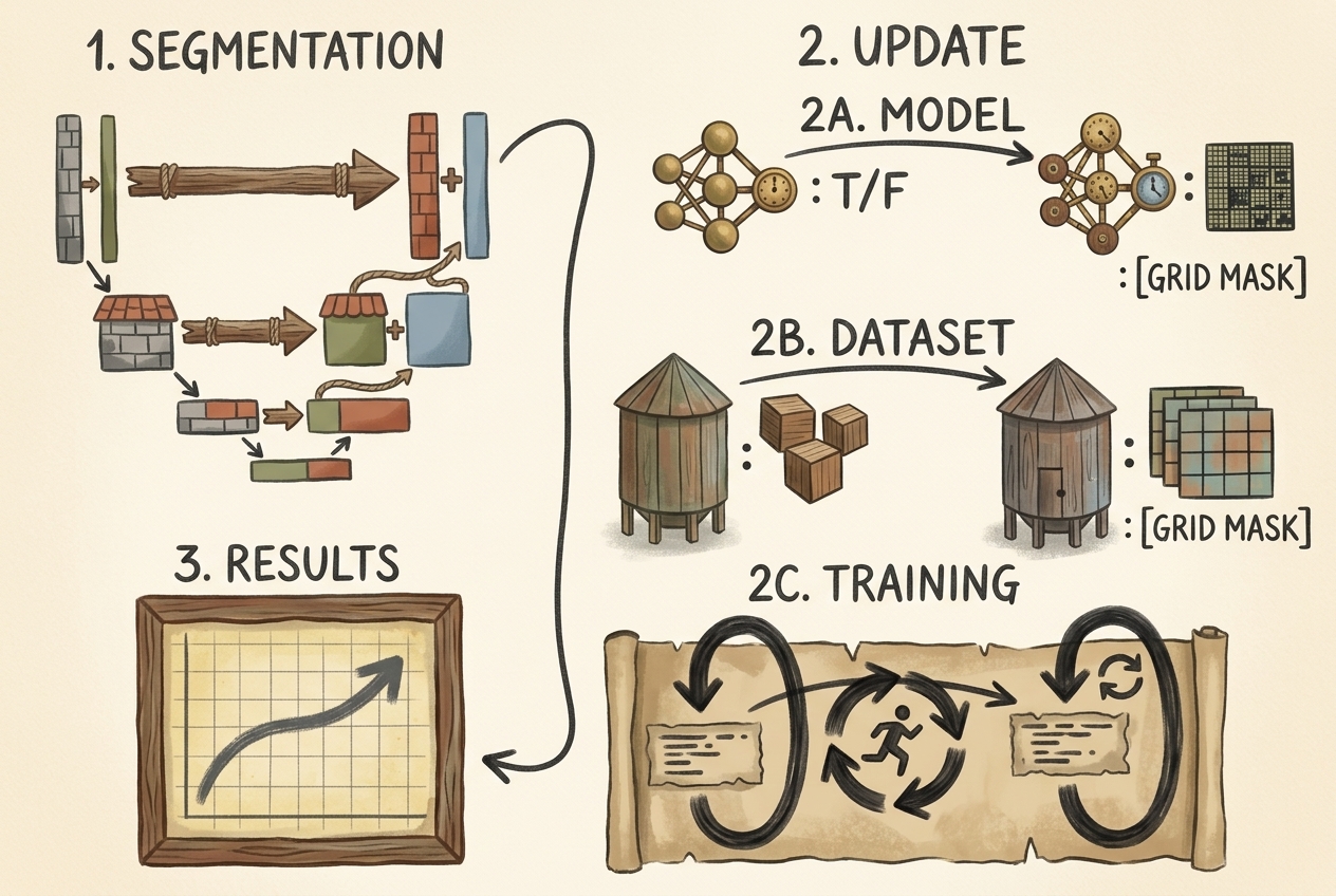
flowchart TD
    subgraph Roadmap ["Section 2.7 Engineering Roadmap"]
        direction TB
        R1["1. Understand Segmentation Mechanics<br/>Per-Pixel Classification vs. Image Tagging"]
        R2A["2A. Model Architecture Selection<br/>Zero-Shot SAM vs. Fine-Tuned SegFormer"]
        R2B["2B. Dataset Pipeline Upgrades<br/>Extracting 2D Axial Slices & Binary Masks"]
        R2C["2C. Training Strategy<br/>Freezing Encoder & Hybrid Dice/BCE Loss"]
        R3["3. Candidate Extraction & Verification<br/>Connected Components to 3D Coordinates"]
        R1 --> R2A --> R2B --> R2C --> R3
    end

    style Roadmap fill:#1a1a2e,stroke:#4cc9f0,stroke-width:2px,color:#fff
    style R1 fill:#16213e,stroke:#4cc9f0,stroke-width:1px,color:#fff
    style R2A fill:#1a3a2a,stroke:#52b788,stroke-width:1px,color:#fff
    style R2B fill:#1a3a2a,stroke:#52b788,stroke-width:1px,color:#fff
    style R2C fill:#1a3a2a,stroke:#52b788,stroke-width:1px,color:#fff
    style R3 fill:#0f3460,stroke:#4cc9f0,stroke-width:2px,color:#fff
3. Classification vs. Semantic Segmentation: The Per-Pixel Spatial Mandate
To understand why a dedicated segmentation model is necessary, consider the difference in output semantics between image-level classification and semantic segmentation.
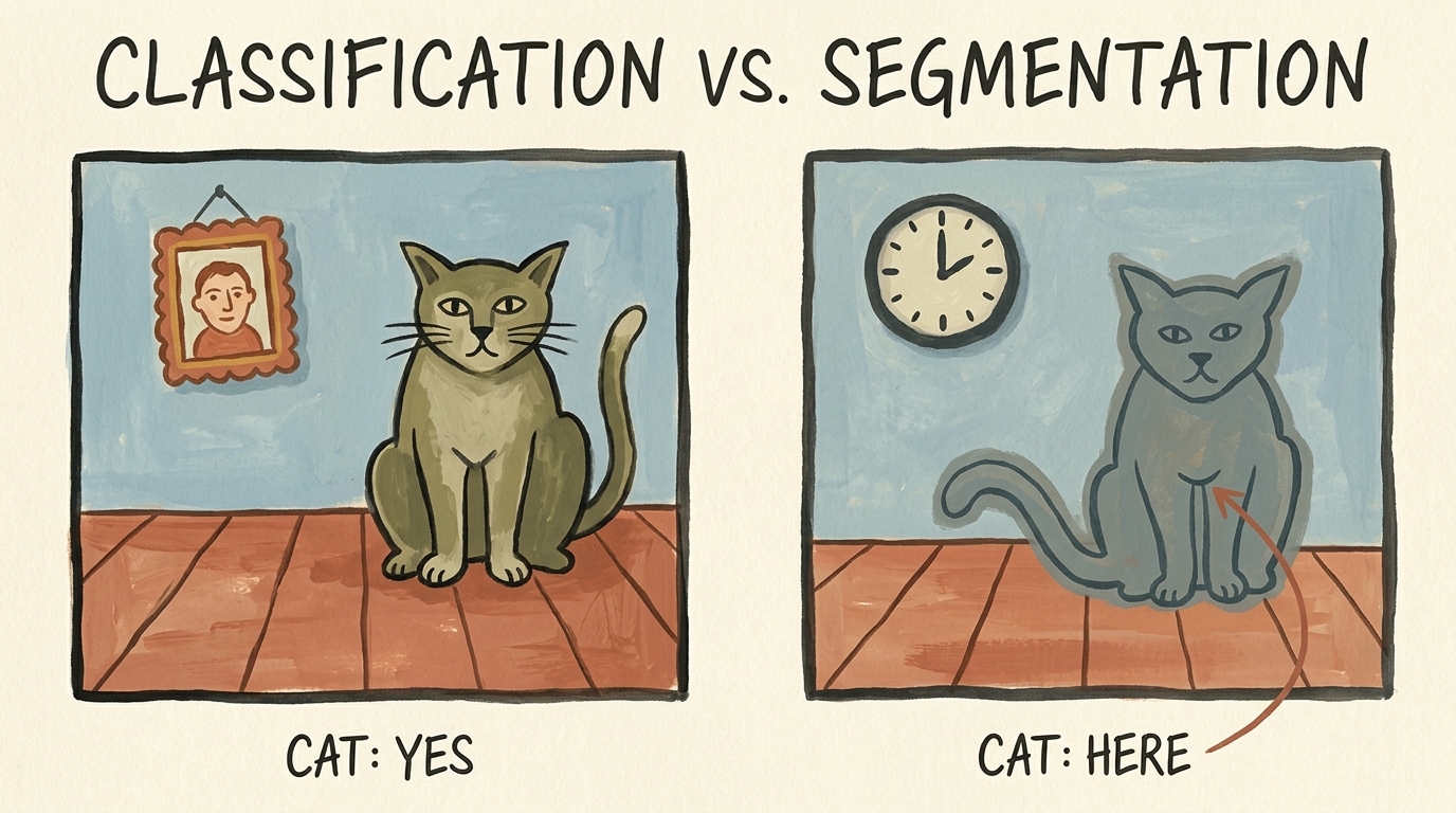
3.1 Mathematical Formulation of Output Spaces
In binary classification, the neural network maps an input image or volumetric tensor $\mathbf{X} \in \mathbb{R}^{C \times H \times W}$ to a single scalar probability representing class membership:
$$ f_{\text{cls}}(\mathbf{X}) = \hat{y} \in [0, 1] $$
In contrast, Semantic Segmentation performs dense, per-pixel (or per-voxel) classification. The network outputs a spatial probability map of identical height and width as the input:
$$ f_{\text{seg}}(\mathbf{X}) = \hat{\mathbf{M}} \in [0, 1]^{H \times W} $$
Where each individual element $\hat{\mathbf{M}}_{i, j}$ represents the conditional probability that pixel $(i, j)$ belongs to the target foreground class (the tumor nodule):
$$ \hat{\mathbf{M}}_{i, j} = P(Y_{i, j} = 1 \mid \mathbf{X}) $$
3.2 The Spatial Bottleneck in Standard Classification Networks
Why can’t we simply use our classification CNN from Section 2.5 to tell us where the nodule is?
Standard classification architectures rely on progressive spatial downsampling (strided convolutions and max pooling) to aggregate spatial contexts into higher-level semantic features (textures $\to$ object parts $\to$ semantic concepts). At the terminal end of the network, a Global Average Pooling or fully connected layer collapses all remaining spatial dimensions into a 1D vector:
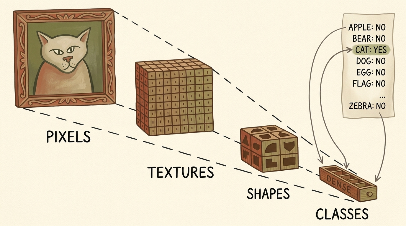
Input: (C, H, W) ──> Conv/Pool ──> (C_1, H/2, W/2) ──> ... ──> (C_k, 1, 1) ──> Linear ──> (K classes)
Once the tensor is collapsed into a 1D vector of logits, spatial coordinates $(x, y)$ are destroyed. To preserve and reconstruct dense spatial coordinates, segmentation architectures require an encoder-decoder topology (such as U-Net or SegFormer) that downsamples for semantic context, then systematically upsamples back to the original resolution while maintaining spatial detail via skip connections or multi-scale attention.
4. Foundation Models in Vision: Meta’s Segment Anything Model (SAM)
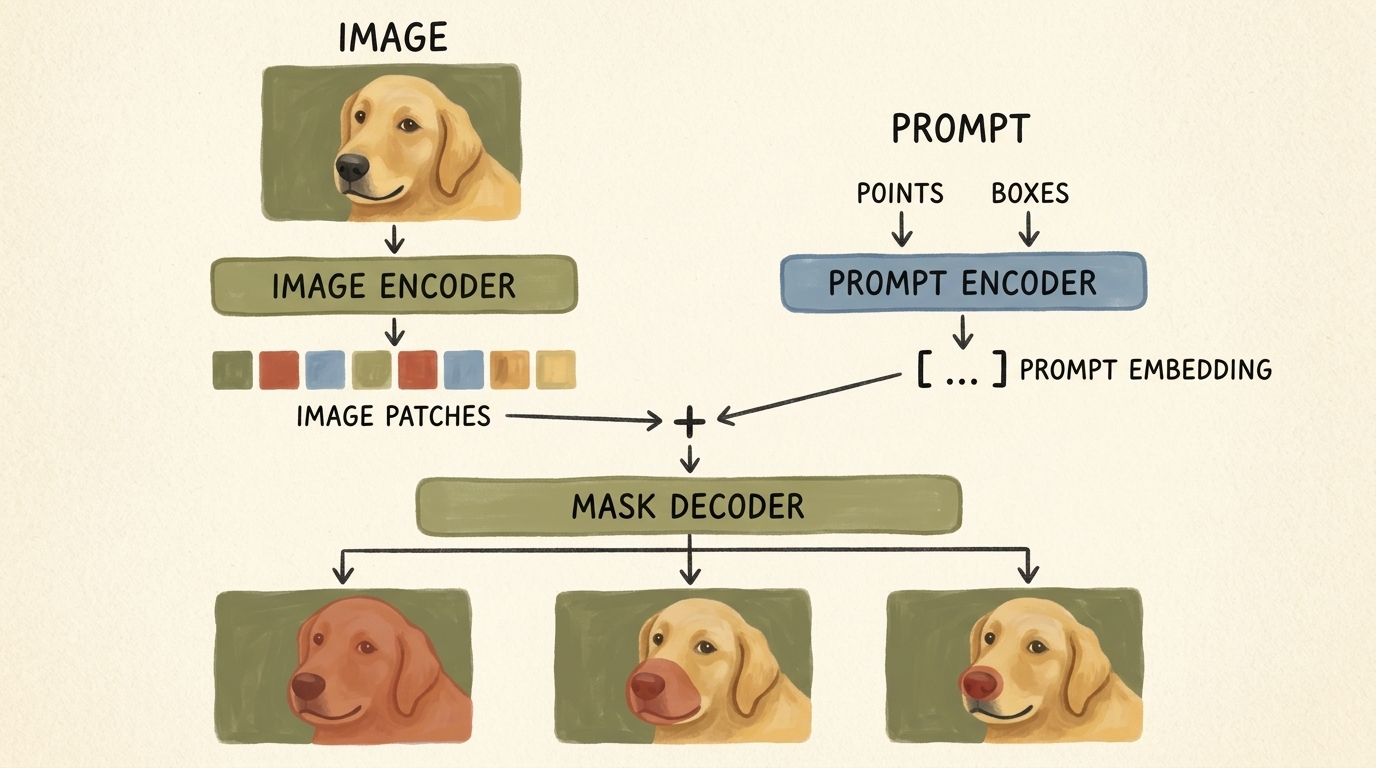
Historically, semantic segmentation required training fully convolutional networks (such as U-Net or DeepLabV3) from scratch on tens of thousands of manually labeled per-pixel masks. In 2023, Meta AI introduced the Segment Anything Model (SAM) (Kirillov et al.), representing a paradigm shift toward promptable foundation models for computer vision.
4.1 SAM Architectural Breakdown
SAM is engineered as a three-component system designed for real-time promptable inference:
-
Image Encoder (Heavy Backbone):
- Built on a Vision Transformer (ViT-B, ViT-L, or ViT-H) pretrained with Masked Autoencoders (MAE).
- Ingests a high-resolution $1024 \times 1024$ image, divides it into $16 \times 16$ non-overlapping patches, and processes them through windowed self-attention blocks.
- Outputs a spatial feature map of shape $64 \times 64 \times 256$ (a $\times 16$ downsampled dense image embedding).
- Computational characteristic: Heavy compute footprint ($\approx 90\text{M}$ to $600\text{M}$ parameters), run only once per image.
-
Prompt Encoder (Lightweight):
- Handles sparse prompts: foreground/background points, bounding boxes, or rough text prompts.
- Points and boxes are encoded using positional embeddings combined with learned embeddings representing point types ($1 = \text{foreground click}, 0 = \text{background click}$).
- Dense mask prompts are embedded via convolutional convolutions.
- Computational characteristic: Extremely lightweight ($< 1\text{ ms}$ on CPU/GPU).
-
Mask Decoder (Real-Time Fusion):
- A two-layer transformer decoder that performs two-way cross-attention: prompt tokens attend to image patch embeddings, and image embeddings attend back to prompt tokens.
- Ambiguity Resolution: A single point prompt can legitimately denote multiple nested objects (e.g., clicking on a dog’s nose could mean the whole dog, the snout, or just the nose tip). SAM’s decoder simultaneously predicts 3 candidate masks at varying granularities along with an estimated IoU score.
4.2 Using SAM Off-the-Shelf for Point-Guided Segmentation
We can invoke SAM to segment anatomical structures zero-shot by providing an interactive point prompt. First, we install the official library from GitHub:
pip install git+https://github.com/facebookresearch/segment-anything.git
We instantiate SAM, load the pretrained weights (sam_vit_b_01ec64.pth), transfer to GPU, and initialize the SamPredictor wrapper:
import torch
from segment_anything import sam_model_registry, SamPredictor

device = torch.device("cuda" if torch.cuda.is_available() else "cpu")

# Load ViT-Base checkpoint (91M parameters)
sam_checkpoint = "sam_vit_b_01ec64.pth"
model_type = "vit_b"

sam = sam_model_registry[model_type](checkpoint=sam_checkpoint)
sam.to(device=device)

# Initialize promptable predictor
predictor = SamPredictor(sam)
5. Volumetric Slicing: Bridging 3D CT Scans to 2D Foundation Models
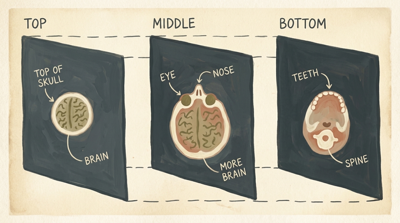
A major architectural challenge in medical computer vision is the dimensional mismatch:
- Vision foundation models (SAM, SegFormer, CLIP, Stable Diffusion) are trained on massive datasets of 2D natural images (e.g., SA-1B contains 11 million 2D images).
- Medical CT scans are 3D volumetric scalar fields ($D \times H \times W$) representing tissue radiodensity.
True 3D foundation models do not exist at the scale of 2D models because 3D volumetric medical datasets are small and 3D memory footprints grow cubically ($O(N^3)$). To exploit the rich representational capacity of 2D foundation models, we systematically partition our 3D CT scans into 2D axial slices along the Z-axis.
5.1 Anatomical Coordinate Transformation
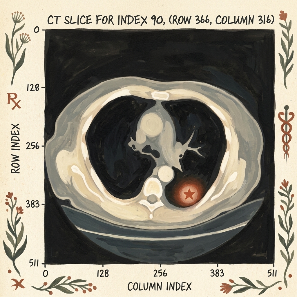
Recall from Section 2.4 that patient coordinates are expressed in millimeters $(x, y, z)_{\text{mm}}$ with respect to an arbitrary scanner origin. To extract the exact 2D axial slice containing a known nodule candidate, we convert the millimeter coordinates into integer voxel indices:
$$ i_z = \left\lfloor \frac{z_{\text{mm}} - z_{\text{origin}}}{s_z} \right\rceil, \quad i_r = \left\lfloor \frac{y_{\text{mm}} - y_{\text{origin}}}{s_y} \right\rceil, \quad i_c = \left\lfloor \frac{x_{\text{mm}} - x_{\text{origin}}}{s_x} \right\rceil $$
Where $s_x, s_y, s_z$ represent the scanner voxel spacing in millimeters.
# Converting millimeter coordinates to discrete voxel index space
slice_ndx = int(round((center_xyz[2] - ct.origin_xyz[2]) / ct.vxSpacing_xyz[2]))
row_ndx = int(round((center_xyz[1] - ct.origin_xyz[1]) / ct.vxSpacing_xyz[1]))
col_ndx = int(round((center_xyz[0] - ct.origin_xyz[0]) / ct.vxSpacing_xyz[0]))

# Extracting a 2D axial slice from the 3D Hounsfield tensor
ct_slice_hu = ct.hu_a[slice_ndx]  # Shape: (512, 512)
5.2 Radiodensity Windowing and Normalization
Raw CT voxels are calibrated in Hounsfield Units (HU), ranging from $-1000\text{ HU}$ (air) to $+1000\text{ HU}$ (dense cortical bone). Because 2D vision models expect normalized inputs in the range $[0, 1]$ or $[0, 255]$, we apply Lung Windowing:
- Window Center (Level): $L = -600\text{ HU}$
- Window Width: $W = 1500\text{ HU}$
- Effective Range: $[-1350\text{ HU}, +150\text{ HU}]$
Any tissue denser than $+150\text{ HU}$ is clipped to 1.0 (white), and any air less than $-1350\text{ HU}$ is clipped to 0.0 (black), maximizing contrast across pulmonary parenchyma and soft nodules.
import numpy as np

def normalize_lung_window(slice_hu, vmin=-1000.0, vmax=400.0):
    """Normalize raw CT Hounsfield Units into [0, 1] range."""
    clipped = np.clip(slice_hu, vmin, vmax)
    normalized = (clipped - vmin) / (vmax - vmin)
    return normalized.astype(np.float32)
6. Building the Segmentation Dataset with SAM Pseudo-Ground-Truth
To train an automated segmentation network, we require paired inputs: an input CT slice $\mathbf{X}$ and a corresponding binary ground-truth mask $\mathbf{Y} \in {0, 1}^{H \times W}$.
While the LUNA dataset provides candidate centroid coordinates $(x, y, z)$ and approximate diameters, it does not provide pixel-level polygon masks for all nodules. Here, we leverage SAM as an annotation assistant:
- We feed the normalized 2D CT slice to SAM’s image encoder.
- We supply the known nodule voxel coordinate $(col, row) = (316, 366)$ as a single positive point prompt.
- SAM segments the exact morphological boundary of the nodule in milliseconds, generating our ground-truth mask $\mathbf{Y}$.
# Format normalized slice as 3-channel uint8 image for SAM
slice_rgb = np.repeat((normalized_slice * 255).astype(np.uint8)[:, :, None], 3, axis=2)

# Pass image to SAM
predictor.set_image(slice_rgb)

# Supply the known nodule coordinate as a positive point prompt (label=1)
point_coords = np.array([[col_ndx, row_ndx]])
point_labels = np.array([1])

# Predict binary masks
masks, scores, logits = predictor.predict(
    point_coords=point_coords,
    point_labels=point_labels,
    multimask_output=True
)

# Select the mask with the highest predicted IoU score
best_mask = masks[np.argmax(scores)]  # Shape: (512, 512), dtype: bool
6.1 Dataset Directory Architecture
We persist these generated slice-mask pairs into a high-performance, structured dataset directory on disk:
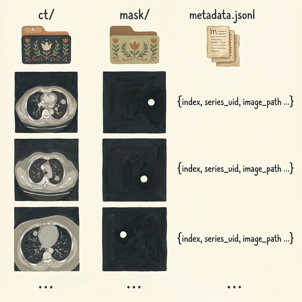
data-segmentation/
├── ct/
│   ├── slice_00090.png
│   ├── slice_00124.png
│   └── ...
├── mask/
│   ├── mask_00090.png
│   ├── mask_00124.png
│   └── ...
└── metadata.jsonl
Each entry in metadata.jsonl stores structured JSON records enabling reproducible train/validation splitting:
{"index": 90, "series_uid": "1.3.6.1.4.1.14519...", "image_path": "ct/slice_00090.png", "mask_path": "mask/mask_00090.png", "row": 366, "col": 316}
7. Fully Automated Unprompted Segmentation with SegFormer
While SAM is exceptional at zero-shot interactive segmentation when prompted with a point or bounding box, it cannot be deployed directly as an autonomous clinical screener. An autonomous scanner must ingest an unannotated CT scan and identify nodules without any human clicking where the nodule is.
For autonomous semantic segmentation, the authors of Deep Learning with PyTorch (2nd Ed) transition to SegFormer (Xie et al., NeurIPS 2021).
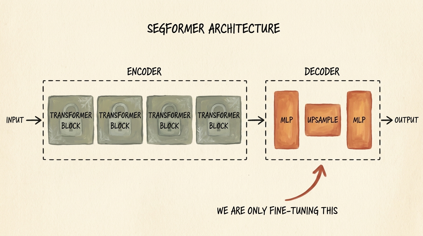
7.1 SegFormer Architecture: Hierarchical Transformer + All-MLP Decoder
SegFormer overcomes the computational bottlenecks of standard Vision Transformers through two core innovations:
-
Hierarchical Mix Transformer (MiT) Encoder:
- Unlike ViT, which generates single-resolution feature maps via fixed patch embeddings, SegFormer uses Overlapping Patch Merging to produce hierarchical multi-scale feature maps at ${1/4, 1/8, 1/16, 1/32}$ of the original resolution.
- It eliminates positional embeddings entirely, using depthwise $3 \times 3$ convolutions directly within feed-forward blocks (Mix-FFN). This allows the model to process variable input resolutions without interpolating positional encodings.
- It uses Efficient Self-Attention: reducing the spatial sequence length of Key and Value matrices by a reduction ratio $R$, reducing attention computational complexity from $\mathcal{O}(N^2)$ to $\mathcal{O}\left(\frac{N^2}{R}\right)$.
-
Lightweight All-MLP Decoder:
- Traditional segmentation decoders (like U-Net) use compute-intensive deconvolutional layers.
- SegFormer’s decoder consists solely of Multi-Layer Perceptrons (MLPs). It projects multi-scale features from the 4 encoder stages to a unified channel dimension $C$, upsamples them bilinearly to $1/4$ resolution, concatenates them, and applies a final linear layer to predict per-pixel class logits.
7.2 Fine-Tuning Strategy: Freezing the Encoder
Because medical imaging datasets are small, training an entire Vision Transformer from scratch risks catastrophic overfitting. We adopt a Parameter-Efficient Fine-Tuning (PEFT) strategy:
- We load the pretrained
nvidia/mit-b0checkpoint (the most lightweight SegFormer variant, with only 3.7 million total parameters). - We freeze all parameters of the MiT encoder, locking its rich visual representation features.
- We fine-tune only the All-MLP Decoder, adapting its terminal projection to medical CT nodule distributions.
from transformers import SegformerForSemanticSegmentation

# Load pretrained SegFormer with 2 output classes: background (0) and nodule (1)
model = SegformerForSemanticSegmentation.from_pretrained(
    "nvidia/mit-b0",
    num_labels=2,
    ignore_mismatched_sizes=True
)

# Freeze all encoder parameters
for param in model.segformer.encoder.parameters():
    param.requires_grad = False

# Verify trainable parameter count
trainable_params = sum(p.numel() for p in model.parameters() if p.requires_grad)
total_params = sum(p.numel() for p in model.parameters())

print(f"Total Parameters: {total_params:,}")
print(f"Trainable Parameters (Decoder Only): {trainable_params:,} ({100 * trainable_params / total_params:.2f}%)")
8. Loss Functions for Extreme Foreground-Background Imbalance: BCE + Dice Loss
In medical segmentation, class imbalance is significantly more severe than in classification. In a $512 \times 512$ CT slice, there are $262{,}144$ pixels. A small lung nodule might measure 10 pixels in diameter, occupying roughly $78$ pixels:
$$ \frac{\text{Nodule Pixels}}{\text{Total Pixels}} = \frac{78}{262{,}144} \approx 0.0003 \quad (0.03%) $$
If we train a segmentation network using standard per-pixel Cross-Entropy Loss, the model quickly realizes it can achieve 99.97% accuracy by predicting background ($0$) for every single pixel.
8.1 Binary Cross-Entropy with Logits
The standard per-pixel classification loss evaluates each pixel independently:
$$ \mathcal{L}_{\text{BCE}}(\mathbf{y}, \hat{\mathbf{p}}) = -\frac{1}{N} \sum_{i=1}^N \left[ y_i \log(\hat{p}_i) + (1 - y_i) \log(1 - \hat{p}_i) \right] $$
Where $y_i \in {0, 1}$ and $\hat{p}_i = \sigma(z_i) \in [0, 1]$. Because the sum is dominated by the $99.97%$ background pixels, the gradients from the few nodule pixels are drowned out.
8.2 Soft Dice Loss (Sørensen–Dice Coefficient)
To directly optimize overlap regardless of class size, we employ Dice Loss, derived from the Sørensen–Dice similarity metric (closely related to Intersection over Union / Jaccard Index):
$$ \text{Dice} = \frac{2 |\mathbf{Y} \cap \hat{\mathbf{P}}|}{|\mathbf{Y}| + |\hat{\mathbf{P}}|} = \frac{2 \sum_{i=1}^N y_i \hat{p}_i}{\sum_{i=1}^N y_i + \sum_{i=1}^N \hat{p}_i} $$
To make this metric differentiable for backpropagation, we formulate the Soft Dice Loss with a Laplace smoothing term $\epsilon = 1.0$ (to prevent division by zero when both prediction and ground truth are empty):
$$ \mathcal{L}_{\text{Dice}}(\mathbf{y}, \hat{\mathbf{p}}) = 1 - \frac{2 \sum_{i=1}^N y_i \hat{p}_i + \epsilon}{\sum_{i=1}^N y_i + \sum_{i=1}^N \hat{p}_i + \epsilon} $$
8.3 The Hybrid Loss: Combining Local and Global Objectives
In practice, combining BCE with Soft Dice Loss yields the most stable convergence:
- BCE provides smooth gradient flow when predictions are completely wrong ($|\mathbf{Y} \cap \hat{\mathbf{P}}| = 0$).
- Dice Loss ensures the network pays equal attention to small nodule boundaries regardless of slice resolution.
$$ \mathcal{L}_{\text{total}} = \mathcal{L}_{\text{BCE}} + \lambda \mathcal{L}_{\text{Dice}} $$
import torch
import torch.nn as nn
import torch.nn.functional as F

class DiceBCELoss(nn.Module):
    """
    Hybrid loss combining Binary Cross-Entropy and Soft Dice Loss
    for highly imbalanced semantic segmentation.
    """
    def __init__(self, dice_weight=1.0, smooth=1.0):
        super().__init__()
        self.dice_weight = dice_weight
        self.smooth = smooth
        self.bce = nn.BCEWithLogitsLoss()

    def forward(self, logits, targets):
        # Flatten batch and spatial dimensions
        logits_flat = logits.view(-1)
        targets_flat = targets.view(-1)

        # Compute Binary Cross Entropy
        bce_loss = self.bce(logits_flat, targets_flat.float())

        # Compute Soft Dice Loss
        probs = torch.sigmoid(logits_flat)
        intersection = (probs * targets_flat).sum()
        dice_loss = 1.0 - (2.0 * intersection + self.smooth) / (
            probs.sum() + targets_flat.sum() + self.smooth
        )

        return bce_loss + self.dice_weight * dice_loss
9. Training, Checkpointing, and Candidate Coordinate Extraction
9.1 Training Loop Implementation
We train our fine-tuned SegFormer using the AdamW optimizer with a learning rate of $5 \times 10^{-4}$ and weight decay of $10^{-2}$.
from torch.optim import AdamW
from torch.utils.data import DataLoader

# Optimizer applied ONLY to trainable parameters (the decoder)
optimizer = AdamW(
    filter(lambda p: p.requires_grad, model.parameters()),
    lr=5e-4,
    weight_decay=1e-2
)

criterion = DiceBCELoss(dice_weight=1.0)
num_epochs = 20

model.to(device)

for epoch in range(1, num_epochs + 1):
    model.train()
    running_train_loss = 0.0

    for batch_images, batch_masks in train_loader:
        batch_images = batch_images.to(device)
        batch_masks = batch_masks.to(device)

        optimizer.zero_grad()

        # Forward pass: SegFormer outputs logits
        outputs = model(pixel_values=batch_images)
        logits = outputs.logits  # Shape: (B, num_classes, H/4, W/4)

        # Bilinearly interpolate logits to match ground-truth resolution (512, 512)
        upsampled_logits = F.interpolate(
            logits,
            size=batch_masks.shape[-2:],
            mode="bilinear",
            align_corners=False
        )

        # Compute loss on nodule class (channel 1)
        loss = criterion(upsampled_logits[:, 1], batch_masks)

        loss.backward()
        optimizer.step()

        running_train_loss += loss.item()

    avg_train_loss = running_train_loss / len(train_loader)
    print(f"Epoch {epoch:02d}/{num_epochs:02d} | Train Loss: {avg_train_loss:.4f}")
9.2 Saving and Loading the Fine-Tuned Checkpoint
Upon completion of 20 epochs, we save the trained state dictionary:
# Save model parameters to disk
torch.save(model.state_dict(), "segformer_nodule_epoch_20.pt")

# Loading for production inference
model.load_state_dict(torch.load("segformer_nodule_epoch_20.pt", map_location=device))
model.eval()
9.3 Candidate Extraction via Connected Component Analysis
Once the model generates a predicted probability map $\hat{\mathbf{M}}$ for an axial slice, we convert the continuous probability map into discrete nodule candidate bounding coordinates:
- Thresholding: Apply a probability cutoff (e.g., $\hat{\mathbf{M}}_{i, j} > 0.5$) to produce a clean binary mask.
- Connected Components: Run
scipy.ndimage.labelor OpenCVcv2.connectedComponentsWithStatsto group contiguous positive pixels into discrete candidate clusters. - Centroid Extraction: Compute the center of mass $(r_c, c_c)$ for each component.
- Coordinate Mapping: Map $(slice_ndx, r_c, c_c)$ back into millimeter space $(x, y, z)_{\text{mm}}$ using voxel spacing.
These extracted candidate coordinates are then fed directly into our Section 2.6 3D classifier, completing the autonomous Computer-Aided Detection pipeline.
10. Summary and Key Insights
- CAD Pipeline Step 2: Candidate proposal via semantic segmentation eliminates the computational impossibility of sliding 3D convolutional classifiers across 100 million voxels, reducing candidate regions to a manageable few dozen.
- Per-Pixel vs Global Semantics: Classification compresses spatial information into 1D class probabilities, destroying coordinate localization. Segmentation preserves spatial dimensions via encoder-decoder topologies.
- Foundation Models in Vision: Meta’s Segment Anything Model (SAM) provides instant zero-shot promptable segmentation for ground-truth mask synthesis when guided by radiologist coordinate clicks.
- 3D to 2D Decomposition: Extracting 2D axial slices along the cranial-caudal Z-axis allows medical pipelines to leverage billion-parameter 2D vision foundation models without requiring impossible 3D memory allocations.
- Autonomous Unprompted Segmentation: Because SAM requires interactive prompts, we fine-tune SegFormer (
nvidia/mit-b0) for fully automated, unprompted semantic segmentation. - Parameter-Efficient Transfer Learning: Freezing the Mix Transformer (MiT) encoder and fine-tuning only the lightweight All-MLP Decoder enables rapid training on a single GPU while preventing overfitting.
- Hybrid Dice + BCE Loss: Combines smooth global gradient flow with direct spatial overlap optimization, resolving the severe $99.97%$ background class imbalance inherent in medical segmentation.