Canny Edge Detector and Corner Detection
- 1. Canny Edge Detector
- 2. Corner Detection (Harris & Moravec Corner Detector)
- 2.1. Why Corners? (2D Constraints & Aperture Problem)
- 2.2. Categorization of Image Neighborhoods
- 2.3. Mathematical Formulation (Sum of Squared Differences & Taylor Series)
- 2.4. Second Moment Matrix ($M$) and Eigenvalue Analysis
- 2.5. Harris Corner Response Function ($R$)
- 2.6. Complete Harris Corner Detection Pipeline
- 3. Summary Comparison of Edge vs Corner Detection
This technical note covers advanced feature extraction techniques in computer vision, focusing on the optimal Canny Edge Detector and Harris Corner Detection (Structure Tensor analysis). We examine their mathematical derivations, multi-scale behavior, spatial autocorrelation, eigenvalue analysis of second moment matrices, and practical algorithmic implementations.
1. Canny Edge Detector
The Canny Edge Detector, developed by John F. Canny in 1986, is widely regarded as the optimal edge detection algorithm for 2D images. It formulates edge detection as an analytical optimization problem subject to precise mathematical constraints.
1.1. John Canny’s Optimization Criteria
Canny defined three fundamental criteria that an optimal edge detector must satisfy:
- Low Error Rate (Optimal Detection): The operator must maximize the signal-to-noise ratio (SNR) by catching all true physical edges while minimizing false positives caused by noise.
- Localization Accuracy: The distance between the detected edge pixel coordinates and the true physical center of the edge boundary must be minimized.
- Single Response Constraint: The detector must return only one pixel-wide response for each single edge boundary, avoiding multiple thick response bands.
flowchart TD
    Raw["Raw Input Image I(x,y)"] --> Step1["1. Gaussian Blur (G_σ * I)\n(Noise Suppression)"]
    Step1 --> Step2["2. Gradient Calculation\n(|∇I| and Angle θ)"]
    Step2 --> Step3["3. Non-Maximum Suppression (NMS)\n(Thinning Edges to 1-Pixel Width)"]
    Step3 --> Step4["4. Hysteresis Dual Thresholding\n(High Thresh Th, Low Thresh Tl)"]
    Step4 --> Step5["5. Edge Tracking by Connectivity\n(Connecting Weak Edges to Strong Edges)"]
    Step5 --> Out["Final Binary Edge Map"]

    style Raw fill:#1a1a2e,stroke:#16213e,color:#fff
    style Step1 fill:#16213e,stroke:#4cc9f0,color:#fff
    style Step2 fill:#16213e,stroke:#4cc9f0,color:#fff
    style Step3 fill:#0f3460,stroke:#e94560,color:#fff
    style Step4 fill:#0f3460,stroke:#e94560,color:#fff
    style Step5 fill:#16213e,stroke:#4cc9f0,color:#fff
    style Out fill:#1a1a2e,stroke:#4cc9f0,color:#fff
1.2. The 5-Step Canny Pipeline
Step 1: Gaussian Smoothing
To suppress high-frequency image noise, the raw image $I(x,y)$ is convolved with a 2D Gaussian kernel $G_\sigma(x,y)$:
$$I_\sigma(x,y) = G_\sigma(x,y) * I(x,y) = \frac{1}{2\pi \sigma^2} e^{-\frac{x^2+y^2}{2\sigma^2}} * I(x,y)$$
Step 2: Gradient Vector Calculation
The smoothed image $I_\sigma$ is processed using Sobel or central difference derivative operators to derive horizontal ($I_x$) and vertical ($I_y$) partial derivatives:
$$|\nabla I| = \sqrt{I_x^2 + I_y^2}, \quad \theta = \tan^{-1} \left( \frac{I_y}{I_x} \right)$$
Step 3: Non-Maximum Suppression (NMS)
NMS thins the thick gradient magnitude response map into crisp, 1-pixel-wide candidate edges. For each pixel $(x,y)$:
- Quantize the gradient direction $\theta(x,y)$ into one of four principal sectors: $0^\circ$ (horizontal), $45^\circ$ (positive diagonal), $90^\circ$ (vertical), or $135^\circ$ (negative diagonal).
- Compare the magnitude $|\nabla I(x,y)|$ with its two immediate neighbors along the gradient normal direction.
- If $|\nabla I(x,y)|$ is smaller than either neighbor, suppress it to zero ($|\nabla I_{NMS}(x,y)| = 0$); otherwise, retain it.
$$\begin{aligned} 0^\circ \text{ Sector:} \quad & \text{Compare with } (x+1, y) \text{ and } (x-1, y) \ 90^\circ \text{ Sector:} \quad & \text{Compare with } (x, y+1) \text{ and } (x, y-1) \ 45^\circ \text{ Sector:} \quad & \text{Compare with } (x+1, y+1) \text{ and } (x-1, y-1) \ 135^\circ \text{ Sector:} \quad & \text{Compare with } (x+1, y-1) \text{ and } (x-1, y+1) \end{aligned}$$
Step 4: Hysteresis Dual Thresholding
To resolve broken edge segments without admitting noisy pixels, two thresholds are applied:
- Strong Edges: $|\nabla I_{NMS}| \ge T_{high} \rightarrow$ Marked as valid edge pixels.
- Weak Edges: $T_{low} \le |\nabla I_{NMS}| < T_{high} \rightarrow$ Candidates for edge connectivity.
- Suppressed: $|\nabla I_{NMS}| < T_{low} \rightarrow$ Rejected.
Step 5: Edge Tracking by Connectivity
A weak edge pixel is preserved if and only if it is connected to a strong edge pixel within an 8-neighbor spatial path. This connected-component analysis prevents edge fragmentation while eliminating isolated noise spikes.
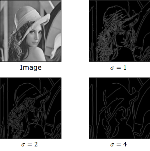
1.3. Multi-Scale Edge Detection ($\sigma$ Parameter)
The standard deviation $\sigma$ of the Gaussian filter acts as a scale-space parameter:
- Small $\sigma$ (Fine Scale): Preserves sharp details, subtle textures, and fine corners, but remains more susceptible to noise.
- Large $\sigma$ (Coarse Scale): Filters out fine textures and noise, highlighting major structural object boundaries, but degrades localization accuracy.
2. Corner Detection (Harris & Moravec Corner Detector)
While edges provide 1D constraints along boundary curves, corners (keypoints / interest points) provide 2D point constraints. A corner is defined as an image location where intensity changes significantly across all 2D spatial directions.
2.1. Why Corners? (2D Constraints & Aperture Problem)
Corners are exceptionally valuable features for camera calibration, 3D reconstruction, optical flow tracking, and object recognition:
- Aperture Problem Mitigation: When viewed through a small local window (aperture), a straight 1D edge suffers from ambiguity along its boundary direction. A corner resolves this ambiguity because its location is constrained in both $x$ and $y$.
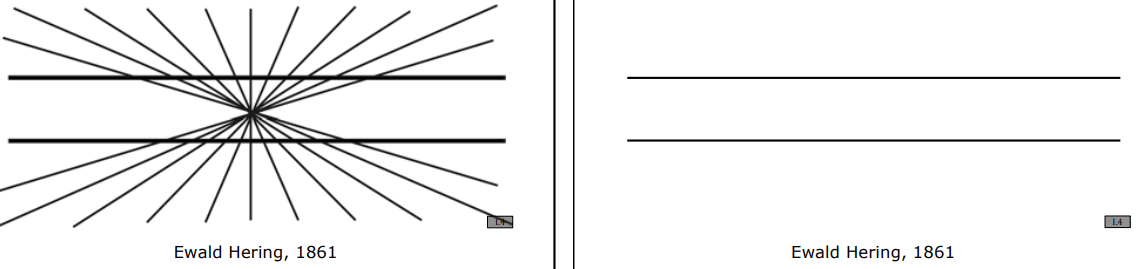
- Perceptual Salience: As demonstrated by visual perception experiments (e.g., Ewald Hering’s 1861 orientation illusion), human vision relies heavily on intersecting lines and corner junctions to perceive structural geometry.
2.2. Categorization of Image Neighborhoods
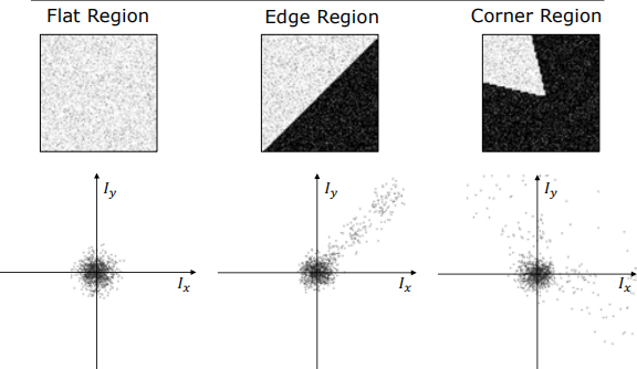
Local image patches are classified into three fundamental geometric categories based on intensity variation when shifting a local window $W$:
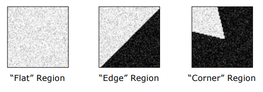
- Flat Region: Shifting the window in any direction results in virtually zero intensity change.
- Edge Region: Shifting the window parallel to the edge direction results in zero intensity change; shifting perpendicular to the edge results in a large intensity change.
- Corner Region: Shifting the window in any spatial direction results in a significant intensity change.
flowchart TD
    Patch["Local Image Window W"] --> ShiftTest["Apply Small Spatial Shift (u,v)"]
    ShiftTest --> Flat["Flat Region\n(No change in any direction)"]
    ShiftTest --> Edge["Edge Region\n(Change in 1 normal direction only)"]
    ShiftTest --> Corner["Corner Region\n(Large change in ALL directions)"]

    style Patch fill:#1a1a2e,stroke:#16213e,color:#fff
    style ShiftTest fill:#16213e,stroke:#4cc9f0,color:#fff
    style Flat fill:#16213e,stroke:#888,color:#fff
    style Edge fill:#0f3460,stroke:#e94560,color:#fff
    style Corner fill:#0f3460,stroke:#4cc9f0,color:#fff
2.3. Mathematical Formulation (Sum of Squared Differences & Taylor Series)
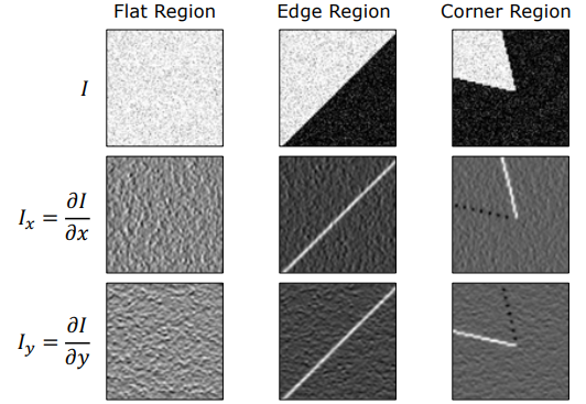
The change in intensity $E(u,v)$ produced by shifting a window $w(x,y)$ by displacement vector $(u,v)$ is formulated using the Sum of Squared Differences (SSD):
$$E(u,v) = \sum_{x,y} w(x,y) \left[ I(x+u, y+v) - I(x,y) \right]^2$$
Where $w(x,y)$ is a window function (either a uniform box window or a 2D Gaussian weighting window $e^{-\frac{x^2+y^2}{2\sigma^2}}$).
Using a first-order 2D Taylor Series expansion for small displacements $(u,v)$:
$$I(x+u, y+v) \approx I(x,y) + u I_x(x,y) + v I_y(x,y)$$
Substituting this back into the SSD equation yields:
$$E(u,v) \approx \sum_{x,y} w(x,y) \left[ u I_x(x,y) + v I_y(x,y) \right]^2$$
Expanding the quadratic term and writing in matrix form:
$$E(u,v) \approx \begin{bmatrix} u & v \end{bmatrix} M \begin{bmatrix} u \[6pt] v \end{bmatrix}$$
Where $M$ is the Second Moment Matrix (also known as the Structure Tensor):
$$M = \sum_{x,y} w(x,y) \begin{bmatrix} I_x^2 & I_x I_y \[6pt] I_x I_y & I_y^2 \end{bmatrix} = \begin{bmatrix} \sum w I_x^2 & \sum w I_x I_y \[6pt] \sum w I_x I_y & \sum w I_y^2 \end{bmatrix}$$
2.4. Second Moment Matrix ($M$) and Eigenvalue Analysis
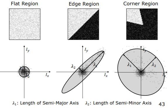
The Second Moment Matrix $M$ summarizes the local gradient distribution inside the window.
Let $\lambda_1$ and $\lambda_2$ be the two eigenvalues of matrix $M$. These eigenvalues represent the principal curvatures of the local auto-correlation quadratic surface $E(u,v)$:
- $\lambda_1$: Length of the semi-major axis of the gradient uncertainty ellipse.
- $\lambda_2$: Length of the semi-minor axis of the gradient uncertainty ellipse.
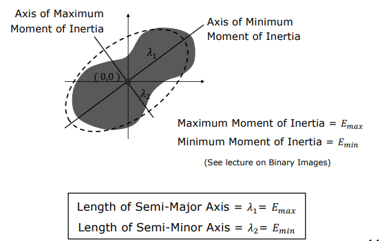
Physical Analogy (Moments of Inertia): As established in binary image geometry, the eigenvalues $\lambda_1$ and $\lambda_2$ correspond to the principal moments of inertia of the local gradient scatter mass: $\lambda_1 = E_{max}$ (maximum moment of inertia) and $\lambda_2 = E_{min}$ (minimum moment of inertia).
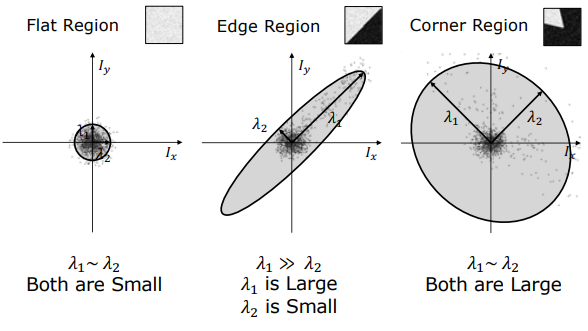
Classification of Image Regions Based on Eigenvalues:
| Region Type | Eigenvalue Relations | Mathematical Condition | Physical Meaning |
|---|---|---|---|
| Flat Region | $\lambda_1 \approx \lambda_2 \approx 0$ | Both $\lambda_1, \lambda_2$ are small | Insignificant gradient variation in any direction. |
| Edge Region | $\lambda_1 \gg \lambda_2 \approx 0$ | One large $\lambda_1$, one near-zero $\lambda_2$ | Strong gradient variation along 1 normal direction only. |
| Corner Region | $\lambda_1 \approx \lambda_2 \gg 0$ | Both $\lambda_1, \lambda_2$ are large | Strong gradient variation in all spatial directions. |
2.5. Harris Corner Response Function ($R$)
Explicitly calculating eigenvalues $\lambda_1, \lambda_2$ for every single pixel requires taking matrix square roots ($\sqrt{b^2 - 4ac}$), which is computationally expensive. Chris Harris and Mike Stephens (1988) devised an elegant scalar response function $R$ using matrix trace and determinant:
$$\det(M) = \lambda_1 \lambda_2 = (\sum w I_x^2)(\sum w I_y^2) - (\sum w I_x I_y)^2$$
$$\operatorname{trace}(M) = \lambda_1 + \lambda_2 = \sum w I_x^2 + \sum w I_y^2$$
The Harris Corner Response $R$ is defined as:
$$R = \det(M) - k \operatorname{trace}(M)^2 = \lambda_1 \lambda_2 - k (\lambda_1 + \lambda_2)^2$$
Where $k$ is an empirical tunable constant, typically set within $0.04 \le k \le 0.06$.
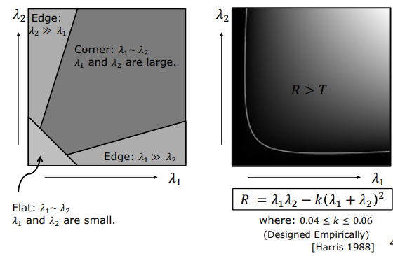
Response Map Partitioning Rules:
- Corner Region: $R > T$ (large positive value).
- Edge Region: $R < -T$ (large negative value, since $\operatorname{trace}(M)^2 \gg \det(M)$).
- Flat Region: $|R| < T$ (small magnitude close to zero).
2.6. Complete Harris Corner Detection Pipeline
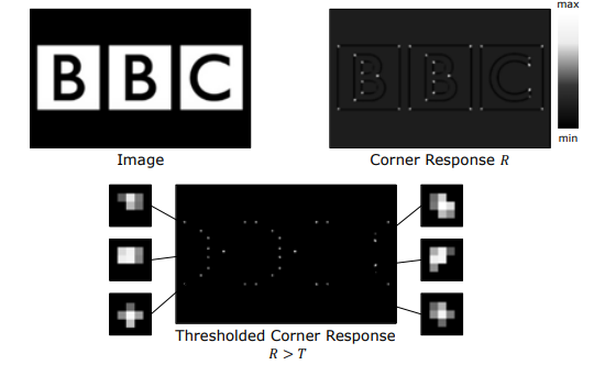
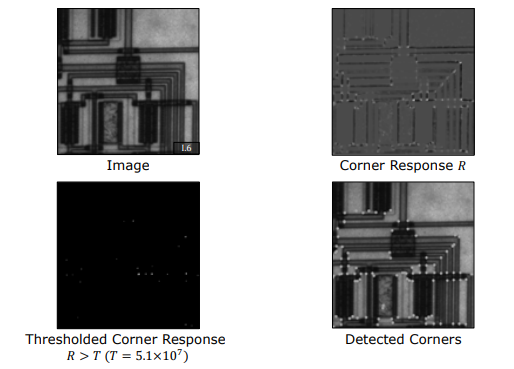
The full Harris Corner Detection algorithm proceeds as follows:
flowchart TD
    Img["Input Image I(x,y)"] --> Grad["Compute Derivatives Ix and Iy\n(using Sobel kernels)"]
    Grad --> Products["Form Derivative Products:\nIx², Iy², IxIy"]
    Products --> Gauss["Apply Gaussian Window W_σ:\nSum w*Ix², Sum w*Iy², Sum w*IxIy"]
    Gauss --> MatrixM["Construct Structure Tensor M"]
    MatrixM --> Resp["Compute Harris Response:\nR = det(M) - k*(trace(M))²"]
    Resp --> Thresh["Thresholding: R > Threshold T"]
    Thresh --> NMS["Non-Maximum Suppression\n(Find local 3x3 peaks)"]
    NMS --> Out["Detected Corner Keypoints"]

    style Img fill:#1a1a2e,stroke:#16213e,color:#fff
    style Grad fill:#16213e,stroke:#4cc9f0,color:#fff
    style Products fill:#16213e,stroke:#4cc9f0,color:#fff
    style Gauss fill:#0f3460,stroke:#e94560,color:#fff
    style MatrixM fill:#0f3460,stroke:#e94560,color:#fff
    style Resp fill:#0f3460,stroke:#e94560,color:#fff
    style Thresh fill:#16213e,stroke:#4cc9f0,color:#fff
    style NMS fill:#16213e,stroke:#4cc9f0,color:#fff
    style Out fill:#1a1a2e,stroke:#4cc9f0,color:#fff
3. Summary Comparison of Edge vs Corner Detection
| Attribute / Property | Canny Edge Detector | Harris Corner Detector |
|---|---|---|
| Constraint Dimension | 1D Spatial Boundary Contours | 2D Point Constraints (Keypoints) |
| Mathematical Basis | Gradient Vector $\nabla I$ + NMS + Hysteresis | Structure Tensor $M$ Eigenvalue Analysis |
| Primary Metric | Gradient Magnitude $ | \nabla I |
| Rotation Invariance | Dependent on gradient quantization | Fully Rotation Invariant (Isotropic Tensor) |
| Scale Sensitivity | Sensitive to Gaussian parameter $\sigma$ | Sensitive to window scale (requires Harris-Laplacian for scale invariance) |
| Primary Applications | Image Segmentation, Object Boundaries | Keypoint Matching, SLAM, Image Stitching, Tracking |