Linear and Non-Linear Image Filters
- 1. Discrete 2D Convolution
- 2. Border Problems
- 3. Classic Linear Filter Types
- 4. Gaussian Smoothing
- 5. Non-Linear Filters
1. Discrete 2D Convolution
In computer vision applications, images are processed as discrete 2D pixel matrices rather than continuous mathematical functions. For an $M \times N$ image $f[i,j]$ and a filter kernel $h[i,j]$, discrete 2D convolution is defined as:
$$g[i,j] = f[i,j] * h[i,j] = \sum_{m} \sum_{n} f[m,n] , h[i - m, j - n]$$
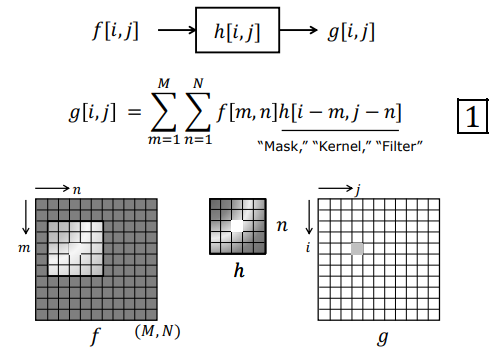
where $i$ represents row indices and $j$ represents column indices.
flowchart TD
    Step1["1. Double Flip: h[-m, -n]"] --> Step2["2. Overlay: Center over pixel f[i,j]"]
    Step2 --> Step3["3. Pointwise Multiplication"]
    Step3 --> Step4["4. Sum -> g[i,j]"]
    Step4 --> Step5["5. Raster Scan Across Image"]
    style Step1 fill:#1a1a2e,stroke:#e94560,color:#fff
    style Step2 fill:#16213e,stroke:#0f3460,color:#fff
    style Step3 fill:#16213e,stroke:#0f3460,color:#fff
    style Step4 fill:#0f3460,stroke:#e94560,color:#fff
    style Step5 fill:#0f3460,stroke:#e94560,color:#fff
1.1 Discrete Convolution Pipeline
Executing discrete 2D convolution follows 5 programmatic steps:
- Double Flip: Flip the filter kernel $h$ horizontally ($m$) and vertically ($n$) to form $h[-m, -n]$.
- Overlay: Center the flipped kernel over target pixel $[i,j]$.
- Multiply: Multiply kernel weights element-wise with overlapping pixel intensity values.
- Sum: Sum all multiplication results and assign the value to output pixel $g[i,j]$.
- Raster Scan: Slide the kernel across the entire image grid from left-to-right and top-to-bottom.
2. Border Problems
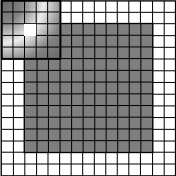
When a filter kernel centers over boundary pixels, portions of the kernel extend beyond the spatial dimensions of the image where no pixel intensity data exists.
flowchart LR
    A["Image Boundary"] --- B["Ignore Border <br/> Cropped Output"]
    A --- C["Constant Padding <br/> Zero Padding"]
    A --- D["Reflection Padding <br/> Mirroring"]
    style A fill:#1a1a2e,stroke:#e94560,color:#fff
    style B fill:#16213e,stroke:#0f3460,color:#fff
    style C fill:#16213e,stroke:#0f3460,color:#fff
    style D fill:#0f3460,stroke:#e94560,color:#fff
Three standard approaches are used to resolve boundary conditions:
2.1 Ignore Border
Compute convolution only for interior pixels where the entire kernel fits strictly inside the image frame. The resulting output image is cropped along its perimeter by the kernel radius.
2.2 Constant / Zero Padding
Pad the regions outside the image boundaries with a constant value (commonly 0 for black or the mean image intensity).
2.3 Reflection Padding
Mirror boundary pixels across the edge boundary. Reflection padding produces the most natural transition and prevents artificial boundary seam artifacts.
3. Classic Linear Filter Types
3.1 Impulse Filter
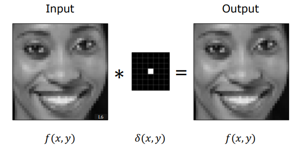
A kernel containing 1 at its center cell and 0 elsewhere passes the input image through unchanged due to the sifting property:
$$g[i,j] = f[i,j] * \delta[i,j] = f[i,j]$$
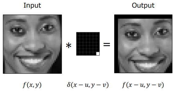
3.2 Shift Filter
Placing the unit impulse at the bottom-right corner of the kernel shifts the output image down and to the right by 1 pixel, due to the double-flip nature of convolution:
$$h = \begin{bmatrix} 0 & 0 & 0 \ 0 & 0 & 0 \ 0 & 0 & 1 \end{bmatrix} \implies g[i,j] = f[i-1, j-1]$$
3.3 Box / Averaging Filter
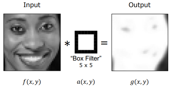
Used to smooth spatial noise across local pixel neighborhoods. Consider an unnormalized $5 \times 5$ box kernel with all entries set to 1:
$$h_{\text{unnorm}} = \begin{bmatrix} 1 & 1 & 1 & 1 & 1 \ \vdots & & \ddots & & \vdots \ 1 & 1 & 1 & 1 & 1 \end{bmatrix}$$
Warning: Saturation and Normalization
Applying an unnormalized box filter causes output pixel values to scale up by $25\times$, exceeding the 8-bit dynamic range (255) and resulting in total white saturation.
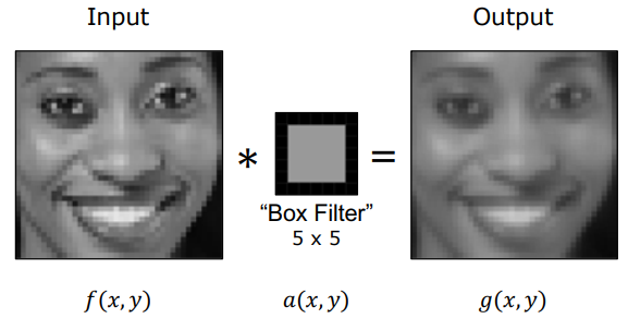
Solution: The sum of all kernel weights must equal 1. Divide each element by the total kernel area ($25$):
$$h_{\text{box}} = \frac{1}{25} \begin{bmatrix} 1 & 1 & 1 & 1 & 1 \ \vdots & & \ddots & & \vdots \ 1 & 1 & 1 & 1 & 1 \end{bmatrix}$$
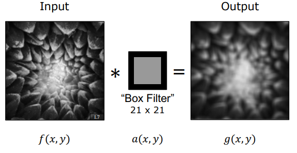
Key Insight: Large box filters (e.g., $21 \times 21$) introduce rectangular boxy artifacts due to sharp square boundaries in spatial domain filtering.
4. Gaussian Smoothing
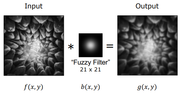
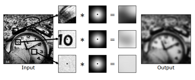
To eliminate rectangular boxy artifacts, Gaussian smoothing uses a rotationally symmetric, smooth kernel whose weights decay gracefully from the center pixel.
4.1 Gaussian Kernel Mathematics
In 2D discrete space, a Gaussian filter kernel is defined as:
$$G_{\sigma}[i,j] = \frac{1}{2\pi\sigma^2} e^{-\frac{i^2 + j^2}{2\sigma^2}}$$
where:
- $i, j$: Row and column spatial distance offsets from the kernel center.
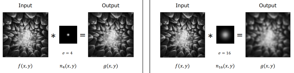
- $\sigma$ (Standard Deviation): Controls kernel spread (smoothing width); $\sigma^2$ represents variance.
- $\frac{1}{2\pi\sigma^2}$: Normalization factor ensuring total volume under the 2D Gaussian sums to 1.
4.2 Kernel Window Size Selection ($K \times K$)
Although continuous Gaussians extend to infinity, finite discrete kernels capture $99.7%$ of Gaussian energy using the standard rule of thumb:
$$K \approx 2\pi\sigma \quad (\text{or } K \approx 6\sigma)$$
4.3 Gaussian Filter Separability
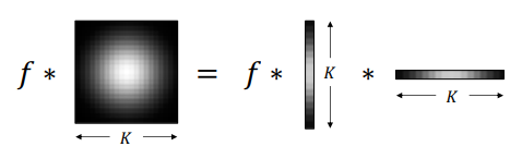
A key property of Gaussian filters in computer vision is separability.
Mathematical Proof
The 2D Gaussian exponent decomposes into the product of two 1D Gaussian exponents:
$$e^{-\frac{m^2 + n^2}{2\sigma^2}} = e^{-\frac{m^2}{2\sigma^2}} \cdot e^{-\frac{n^2}{2\sigma^2}}$$
Substituting into the discrete 2D convolution equation:
$$g[i,j] = \sum_{m} \sum_{n} f[m,n] \cdot \left( \frac{1}{2\pi\sigma^2} e^{-\frac{(i-m)^2 + (j-n)^2}{2\sigma^2}} \right)$$
$$g[i,j] = \frac{1}{2\pi\sigma^2} \sum_{m} e^{-\frac{(i-m)^2}{2\sigma^2}} \left( \sum_{n} f[m,n] \cdot e^{-\frac{(j-n)^2}{2\sigma^2}} \right)$$
Convolving an image with a $K \times K$ 2D Gaussian kernel is mathematically identical to applying a 1D horizontal Gaussian filter of length $K$, followed by a 1D vertical Gaussian filter of length $K$:
$$\text{2D } G_{\sigma} \equiv \text{1D Horizontal } G_{\sigma} * \text{1D Vertical } G_{\sigma}$$
flowchart LR
    A["Image f[i,j]"] --> B["1D Horizontal Gaussian <br/> (K multiplications)"]
    B --> C["1D Vertical Gaussian <br/> (K multiplications)"]
    C --> D["Output g[i,j]"]
    style A fill:#1a1a2e,stroke:#e94560,color:#fff
    style B fill:#16213e,stroke:#0f3460,color:#fff
    style C fill:#16213e,stroke:#0f3460,color:#fff
    style D fill:#0f3460,stroke:#e94560,color:#fff
Computational Complexity Comparison (Per Pixel)
For a $K \times K$ filter window:
- Non-Separable Direct 2D Filter:
- Multiplications: $K^2$
- Additions: $K^2 - 1$
- Separable 1D + 1D Filter:
- Multiplications: $2K$
- Additions: $2(K - 1)$
Performance Optimization Example ($K = 21$):
- Direct 2D: $21^2 = 441$ multiplications, $440$ additions.
- Separable 1D + 1D: $2 \times 21 = 42$ multiplications, $40$ additions.
Speedup: Approximately $10.5\times$ fewer operations per pixel!
5. Non-Linear Filters
Linear convolution filters suppress noise by attenuating high spatial frequencies, which inadvertently blurs sharp object edges. Non-linear algorithmic filters overcome this trade-off.
5.1 Median Filter
Random black (0) or white (255) corrupted pixels are referred to as Salt and Pepper Noise.
flowchart TD
    Sub1["1. Extract K x K Neighborhood"] --> Sub2["2. Sort Pixel Values Ascending"]
    Sub2 --> Sub3["3. Select Median (Middle) Value"]
    Sub3 --> Sub4["4. Assign Median to Target Pixel"]
    style Sub1 fill:#1a1a2e,stroke:#e94560,color:#fff
    style Sub2 fill:#16213e,stroke:#0f3460,color:#fff
    style Sub3 fill:#0f3460,stroke:#e94560,color:#fff
    style Sub4 fill:#0f3460,stroke:#e94560,color:#fff
- Linear Filter Limitation: Gaussian or box filters smear outlier impulse values across neighborhoods, muddying the image without removing noise spikes.
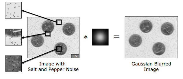
- Median Filter Mechanism: Sort all pixel intensities within a $K \times K$ local window in ascending order and assign the median value to the output pixel.
- Why It Works: Outlier salt (255) and pepper (0) values sit at the extreme ends of sorted lists, making their selection as median values statistically impossible. Noise is removed cleanly without degrading edges.
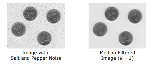
- Drawback: Excessively large median window sizes (e.g., $11 \times 11$) produce watercolor/painterly artifacts that destroy fine detail.
5.2 Bilateral Filter
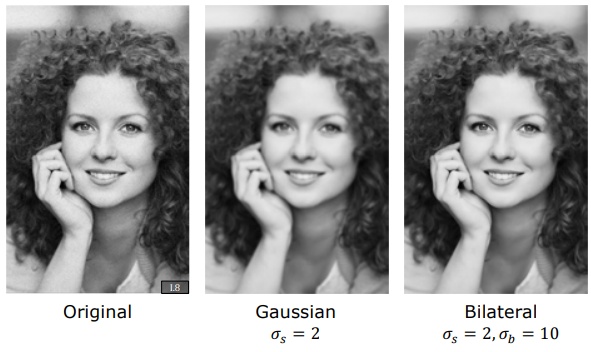
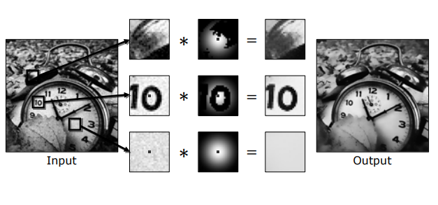
The Bilateral Filter is an edge-preserving non-linear filter that smooths noise in uniform spatial regions while preserving sharp high-frequency edges.
flowchart LR
    Gs["Spatial Gaussian Gs <br/> (Physical Distance)"] --> Mult["Product <br/> Gs x Gr"]
    Gr["Range Gaussian Gr <br/> (Intensity Difference)"] --> Mult
    Mult --> Out["Edge-Preserving Kernel"]
    style Gs fill:#1a1a2e,stroke:#e94560,color:#fff
    style Gr fill:#16213e,stroke:#0f3460,color:#fff
    style Mult fill:#0f3460,stroke:#e94560,color:#fff
    style Out fill:#0f3460,stroke:#e94560,color:#fff
Dual Gaussian Mechanism
Standard Gaussian smoothing relies solely on spatial proximity ($G_s$), whereas Bilateral filtering weights pixels by both spatial proximity ($G_s$) and intensity similarity ($G_r$):
$$g[i,j] = \frac{1}{W[i,j]} \sum_{m} \sum_{n} f[i-m, j-n] \cdot G_s[m,n] \cdot G_r[m,n]$$
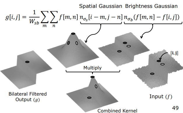
where:
-
Spatial Gaussian ($G_s$): Weights pixels based on geometric distance:
$$G_s[m,n] = e^{-\frac{m^2 + n^2}{2\sigma_s^2}}$$
-
Range / Brightness Gaussian ($G_r$): Weights pixels based on photometric intensity differences relative to the central pixel:
$$G_r[m,n] = e^{-\frac{(f[i-m, j-n] - f[i,j])^2}{2\sigma_r^2}}$$
Dynamic Normalization Factor ($W[i,j]$)
Because kernel weights truncate near sharp boundaries ($G_r \to 0$ across step edges), the normalization constant is recalculated at every pixel position to maintain unit kernel energy:
$$W[i,j] = \sum_{m} \sum_{n} G_s[m,n] \cdot G_r[m,n]$$
Edge-Preserving Intuition
When the kernel centers near a step edge:
- Pixels on the same side of the boundary share similar intensity values $\implies G_r \approx 1$.
- Pixels on the opposite side of the boundary differ significantly in intensity $\implies G_r \approx 0$.
- Result: The kernel truncates along boundary edges, preventing blurring across edge transitions.
Parameter Limiting Behavior
- Increasing $\sigma_s$ increases smoothing across uniform regions.
- As $\sigma_r \to \infty$, $G_r[m,n] \to 1$, reducing the Bilateral filter directly to a standard linear Gaussian filter.
5.3 Comparison: Gaussian vs. Bilateral Filtering