Overview, Fourier Transform, and Convolution Theorem
- 1. Overview of Frequency Domain
- 2. Fourier Transform
- 3. Square Wave Construction & Fourier Series
- 4. Mathematical Formulation and Proofs
- 5. Complex Structure of Fourier Transform
- 6. Fundamental Fourier Transform Pairs
- 7. Fundamental Properties of Fourier Transform
- 8. Convolution Theorem
1. Overview of Frequency Domain
Analyzing images exclusively in the spatial domain (pixel-by-pixel intensity operations) can be computationally expensive and conceptually complex for operations like blurring, sharpening, or deconvolution. The frequency domain provides an alternative representation by expressing spatial image structures as a weighted sum of sinusoids (sine and cosine waves) across various spatial frequencies.
flowchart TD
    A["Spatial Domain Image <br/> f(x,y)"] -->|"Fourier Transform <br/> (Forward FT)"| B["Frequency Domain <br/> F(u,v)"]
    B -->|"Frequency Filtering <br/> H(u,v)"| C["Filtered Spectrum <br/> G(u,v)"]
    C -->|"Inverse Fourier Transform <br/> (Inverse FT)"| D["Enhanced Image <br/> g(x,y)"]
    style A fill:#1a1a2e,stroke:#e94560,color:#fff
    style B fill:#16213e,stroke:#0f3460,color:#fff
    style C fill:#0f3460,stroke:#e94560,color:#fff
    style D fill:#16213e,stroke:#4cc9f0,color:#fff
Transitioning from spatial coordinates to frequency representation yields three core engineering advantages:
- Convolution Efficiency: Computationally intensive spatial convolution integrals are converted into simple point-wise multiplication in the frequency domain.
- Frequency Separation: High-frequency components (fine details, sharp edges, granular noise) and low-frequency components (smooth backgrounds, slow intensity gradients) are explicitly isolated in separate spectral regions.
- Restoration & Deconvolution Stability: Image restoration, motion deblurring, and inverse filtering become mathematically tractable and stable.
Key Insight: Spatial domain operations observe where intensity changes occur, while frequency domain operations analyze how fast intensity changes occur across space.
2. Fourier Transform
The Fourier Transform is named after the French mathematician and physicist Jean Baptiste Joseph Fourier (1768–1830).
2.1 Historical Background
Fourier introduced his foundational concept while modeling heat diffusion through solid materials. He claimed that any periodic function could be represented as an infinite sum of sinusoidal waves.
Prominent mathematicians of his era—including Joseph-Louis Lagrange and Leonhard Euler—initially rejected Fourier’s work as lacking mathematical rigor. It took nearly eight years for his papers to achieve publication. Today, the Fourier Transform serves as a fundamental pillar across signal processing, computer vision, communications, and physics.
2.2 Fundamental Principle: Sinusoidal Building Blocks
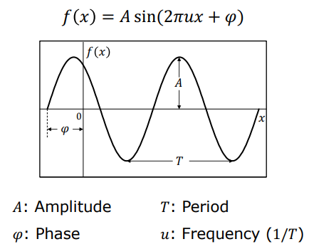
At the heart of Fourier analysis lies the sinusoid. A continuous 1D sinusoidal signal is mathematically defined as:
$$f(x) = A \sin(2\pi u x + \phi)$$
where:
- $A$ (Amplitude): Represents the peak height or maximum power of the wave.
- $u$ (Frequency): Dictates the number of oscillation cycles per unit spatial distance.
- $T = \frac{1}{u}$ (Period): Represents the spatial distance required for one complete oscillation cycle.
- $\phi$ (Phase): Specifies the angular phase shift relative to the origin.
3. Square Wave Construction & Fourier Series
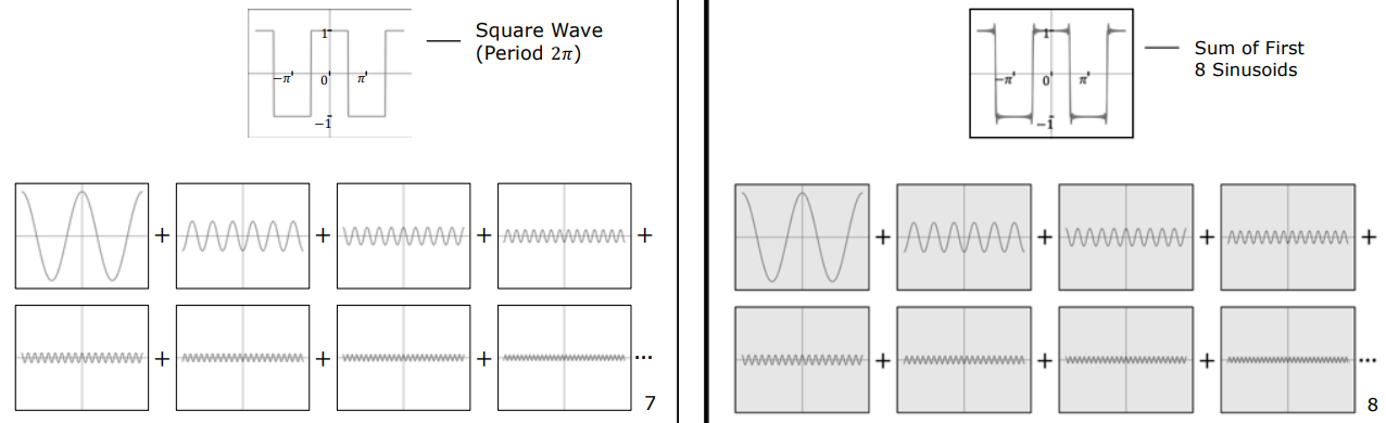
A classic illustration of Fourier theory is constructing a periodic square wave by summing simple sine waves at fundamental and harmonic frequencies.
flowchart LR
    A["Fundamental Sinusoid <br/> u"] --> B["Add 3rd Harmonic <br/> 3u"]
    B --> C["Add 5th & 7th Harmonics <br/> 5u, 7u"]
    C --> D["Infinite Harmonics <br/> N → ∞"]
    D --> E["Ideal Square Wave"]
    style A fill:#1a1a2e,stroke:#e94560,color:#fff
    style B fill:#16213e,stroke:#0f3460,color:#fff
    style C fill:#0f3460,stroke:#e94560,color:#fff
    style D fill:#16213e,stroke:#4cc9f0,color:#fff
    style E fill:#0f3460,stroke:#4cc9f0,color:#fff
- 1 Sinusoid: Adding only the fundamental frequency $u$ yields a coarse, smooth approximation of the square wave.
- Successive Odd Harmonics: Adding odd harmonics ($u, 3u, 5u, 7u, \dots$) with progressively decreasing amplitudes ($\frac{1}{1}, \frac{1}{3}, \frac{1}{5}, \frac{1}{7}, \dots$) flattens the wave crests and steepens vertical transitions.
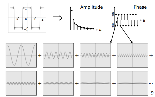
- 8 Sinusoids: Summing the first 8 harmonic terms produces a profile that closely resembles a sharp square wave.
- Infinite Terms: Summing an infinite series of sinusoids yields an exact square wave with perfectly vertical step discontinuities.
Warning: Ringing Artifacts & Gibbs Phenomenon
Representing an instantaneous spatial step discontinuity (such as the vertical edge of a square wave) requires infinitely high frequencies. Truncating the Fourier series to a finite number of harmonics introduces high-frequency oscillations near sharp boundaries, known as ringing artifacts or the Gibbs Phenomenon. Additionally, the phase $\phi$ of harmonics in a square wave alternates between $-\pi/2$ and $\pi/2$.
4. Mathematical Formulation and Proofs
The Fourier Transform maps a continuous spatial signal $f(x)$ to its frequency domain representation $F(u)$ without any loss of information.
4.1 1D Continuous Fourier Transform (Forward & Inverse)
The Forward Fourier Transform (1D FT) converts a spatial function $f(x)$ into the frequency domain $F(u)$:
$$F(u) = \int_{-\infty}^{\infty} f(x) e^{-i 2\pi u x} , dx$$
The Inverse Fourier Transform (1D IFT) reconstructs the original spatial signal $f(x)$ from its frequency spectrum $F(u)$:
$$f(x) = \int_{-\infty}^{\infty} F(u) e^{i 2\pi u x} , du$$
where $x$ denotes spatial position and $u$ represents spatial frequency.
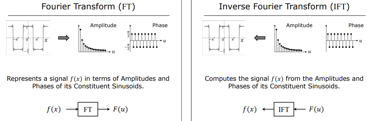
Mathematical Symmetry Note: The forward transform uses $-i$ in the complex exponential exponent, whereas the inverse transform uses $+i$.
4.2 Derivation of Euler’s Formula via Taylor Series
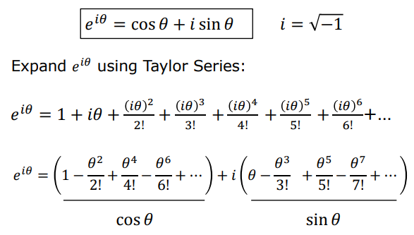
To understand why complex exponentials ($e^{i\theta}$) represent sinusoidal waves ($\cos\theta, \sin\theta$), we use Euler’s Formula:
$$e^{i\theta} = \cos\theta + i\sin\theta \quad (\text{where } i = \sqrt{-1})$$
Step-by-Step Proof:
The Maclaurin (Taylor series around $x=0$) expansion for $e^x$ is:
$$e^{x} = 1 + x + \frac{x^2}{2!} + \frac{x^3}{3!} + \frac{x^4}{4!} + \frac{x^5}{5!} + \dots$$
Substituting $x = i\theta$:
$$e^{i\theta} = 1 + (i\theta) + \frac{(i\theta)^2}{2!} + \frac{(i\theta)^3}{3!} + \frac{(i\theta)^4}{4!} + \frac{(i\theta)^5}{5!} + \dots$$
Using powers of $i$ ($i^2 = -1, i^3 = -i, i^4 = 1, i^5 = i$):
$$e^{i\theta} = 1 + i\theta - \frac{\theta^2}{2!} - i\frac{\theta^3}{3!} + \frac{\theta^4}{4!} + i\frac{\theta^5}{5!} - \dots$$
Group real terms and imaginary terms separately:
$$e^{i\theta} = \left( 1 - \frac{\theta^2}{2!} + \frac{\theta^4}{4!} - \dots \right) + i \left( \theta - \frac{\theta^3}{3!} + \frac{\theta^5}{5!} - \dots \right)$$
Comparing these series with standard Taylor series expansions:
- $\cos\theta = 1 - \frac{\theta^2}{2!} + \frac{\theta^4}{4!} - \dots$
- $\sin\theta = \theta - \frac{\theta^3}{3!} + \frac{\theta^5}{5!} - \dots$
Substituting both yields Euler’s Formula:
$$e^{i\theta} = \cos\theta + i\sin\theta \quad \blacksquare$$
5. Complex Structure of Fourier Transform
Because a Fourier coefficient $F(u)$ must encode both the amplitude (strength) and phase (spatial shift) of frequency $u$, $F(u)$ is inherently a complex number ($F(u) \in \mathbb{C}$):
$$F(u) = \Re(F(u)) + i \Im(F(u))$$
5.1 Magnitude (Amplitude Spectrum)
The magnitude spectrum $|F(u)|$ measures the power or energy of frequency $u$:
$$|F(u)| = \sqrt{\Re(F(u))^2 + \Im(F(u))^2}$$
5.2 Phase Spectrum
The phase spectrum $\phi(u)$ measures spatial alignment or origin offset:
$$\phi(u) = \tan^{-1}\left( \frac{\Im(F(u))}{\Re(F(u))} \right) \quad (\text{computed using } \text{atan2}(\Im, \Re))$$
Negative Frequencies: The integral limits extend from $-\infty$ to $+\infty$. Negative frequencies ($u < 0$) arise naturally from Euler’s formula to maintain Hermitian mathematical symmetry for real-valued spatial signals.
6. Fundamental Fourier Transform Pairs
Below is a reference summary of canonical spatial functions $f(x)$ and their corresponding Fourier transforms $F(u)$:
6.1 Cosine Function
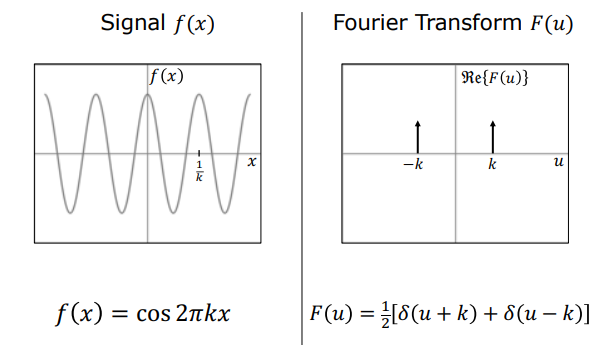
A single pure cosine $f(x) = \cos(2\pi k x)$ contains only frequency $k$. Its Fourier transform consists of two symmetric Dirac delta impulses on the real axis at $u = \pm k$:
$$\mathcal{F}{\cos(2\pi k x)} = \frac{1}{2} \left[ \delta(u - k) + \delta(u + k) \right]$$
6.2 Sum of Cosines
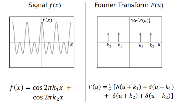
A signal composed of two cosines $f(x) = \cos(2\pi k_1 x) + \cos(2\pi k_2 x)$ produces four delta impulses located at $u = \pm k_1$ and $u = \pm k_2$.
6.3 Sine Function
$f(x) = \sin(2\pi k x)$ also contains frequency $k$, but its delta impulses lie on the imaginary axis with opposite signs:
$$\mathcal{F}{\sin(2\pi k x)} = \frac{i}{2} \left[ \delta(u + k) - \delta(u - k) \right]$$
6.4 Constant Function
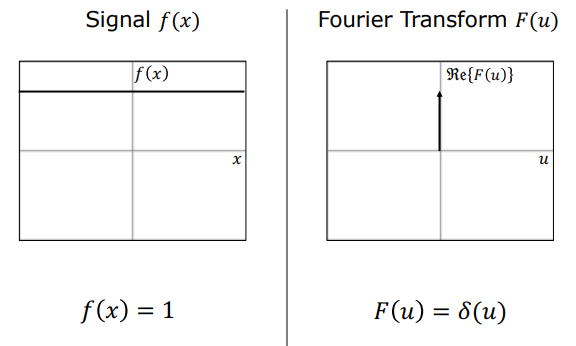
A constant DC signal $f(x) = 1$ has zero spatial variation (zero frequency). Its spectrum is a single Dirac impulse at the origin $u = 0$:
$$\mathcal{F}{1} = \delta(u)$$
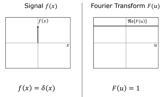
6.5 Unit Impulse (Dirac Delta) Function
A point impulse $f(x) = \delta(x)$ requires equal contributions across all frequencies to form its infinite spatial spike. Its Fourier transform is completely flat:
$$\mathcal{F}{\delta(x)} = 1$$
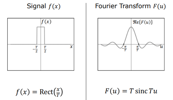
6.6 Rectangular Window Function
A spatial boxcar / rectangle function $f(x) = \text{Rect}(x/T)$ of width $T$ transforms into a Sinc function:
$$\mathcal{F}{\text{Rect}(x/T)} = T \cdot \text{sinc}(Tu) = T \frac{\sin(\pi T u)}{\pi T u}$$
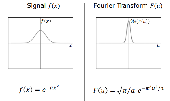
6.7 Gaussian Function
A spatial Gaussian $f(x) = e^{-ax^2}$ with variance parameter $a$ transforms into another Gaussian in the frequency domain:
$$\mathcal{F}{e^{-ax^2}} = \sqrt{\frac{\pi}{a}} e^{-\frac{\pi^2 u^2}{a}}$$
6.8 Inverse Scaling Principle
As demonstrated by the Gaussian and Rect-Sinc pairs, stretching a signal spatially causes it to contract in the frequency domain, and vice versa:
$$f(ax) \iff \frac{1}{|a|} F\left(\frac{u}{a}\right)$$
7. Fundamental Properties of Fourier Transform
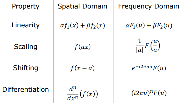
| Property | Spatial Domain ($f(x)$) | Frequency Domain ($F(u)$) | Technical Description |
|---|---|---|---|
| Linearity | $\alpha f_1(x) + \beta f_2(x)$ | $\alpha F_1(u) + \beta F_2(u)$ | Superposition and scaling principles hold in both domains. |
| Scaling | $f(ax)$ | $\frac{1}{|a|} F\left(\frac{u}{a}\right)$ | Spatial expansion causes frequency compression. |
| Shifting | $f(x - a)$ | $F(u) e^{-i 2\pi u a}$ | Spatial translation alters phase without affecting magnitude. |
| Differentiation | $\frac{d^n f(x)}{dx^n}$ | $(i 2\pi u)^n F(u)$ | Taking spatial derivatives amplifies high frequencies (sharpening). |
8. Convolution Theorem
Continuous 1D spatial convolution ($*$) between an image signal $f(x)$ and a system filter $h(x)$ is defined as:
$$g(x) = f(x) * h(x) = \int_{-\infty}^{\infty} f(\tau) h(x - \tau) , d\tau$$
Graphically, spatial convolution involves flipping the filter kernel $h(\tau) \to h(-\tau)$, shifting it by offset $x$, multiplying by $f(\tau)$, and integrating the overlapping area. For example, convolving two identical rectangular boxcars produces a symmetric triangle function.
8.1 Theorem Statement
The Convolution Theorem links spatial operations to frequency operations:
$$\mathcal{F}{f(x) * h(x)} = F(u) \cdot H(u)$$
$$\mathcal{F}{f(x) \cdot h(x)} = F(u) * H(u)$$
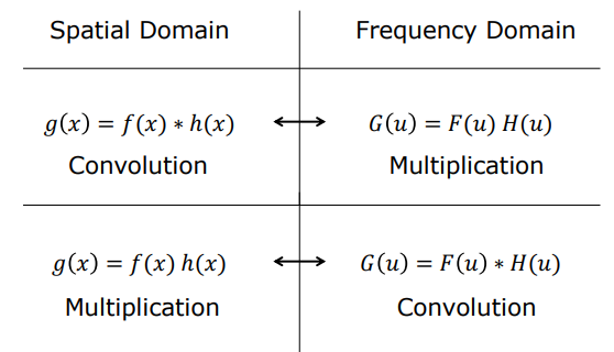
- Spatial Convolution $\iff$ Frequency Multiplication: Convolving two signals in space is equivalent to point-wise multiplying their Fourier transforms in frequency.
- Spatial Multiplication $\iff$ Frequency Convolution: Point-wise multiplying two signals in space is equivalent to convolving their Fourier transforms in frequency.
8.2 Mathematical Proof of Convolution Theorem
We evaluate the Fourier transform $G(u)$ of the spatial convolution output $g(x) = f(x) * h(x)$:
$$G(u) = \int_{-\infty}^{\infty} g(x) e^{-i 2\pi u x} , dx$$
Substitute the spatial convolution integral into $g(x)$:
$$G(u) = \int_{-\infty}^{\infty} \left[ \int_{-\infty}^{\infty} f(\tau) h(x - \tau) , d\tau \right] e^{-i 2\pi u x} , dx$$
Exchange integration order and expand the complex exponential by introducing $+u\tau - u\tau$:
$$e^{-i 2\pi u x} = e^{-i 2\pi u (x - \tau)} e^{-i 2\pi u \tau}$$
Reorganizing the inner and outer integrals:
$$G(u) = \int_{-\infty}^{\infty} f(\tau) e^{-i 2\pi u \tau} \left[ \int_{-\infty}^{\infty} h(x - \tau) e^{-i 2\pi u (x - \tau)} , dx \right] d\tau$$
Apply change of variables $y = x - \tau$ (hence $dy = dx$). Because $\tau$ is finite, integration limits remain $[-\infty, \infty]$:
$$G(u) = \left( \int_{-\infty}^{\infty} f(\tau) e^{-i 2\pi u \tau} , d\tau \right) \cdot \left( \int_{-\infty}^{\infty} h(y) e^{-i 2\pi u y} , dy \right)$$
The first integral is the exact definition of $F(u)$, and the second integral is $H(u)$:
$$G(u) = F(u) \cdot H(u) \quad \blacksquare$$
8.3 Computational Efficiency and Engineering Impact
Convolving an $N \times N$ image with a large spatial filter kernel has $O(N^2)$ computational complexity per pixel. By leveraging the Convolution Theorem and the Fast Fourier Transform (FFT):
flowchart LR
    F_space["Spatial Signals <br/> f(x), h(x)"] -->|"FFT"| F_freq["Spectra <br/> F(u), H(u)"]
    F_freq -->|"Multiply: F(u) · H(u)"| G_freq["Output Spectrum <br/> G(u)"]
    G_freq -->|"IFFT"| G_space["Output Image <br/> g(x)"]
    style F_space fill:#1a1a2e,stroke:#e94560,color:#fff
    style F_freq fill:#16213e,stroke:#0f3460,color:#fff
    style G_freq fill:#0f3460,stroke:#e94560,color:#fff
    style G_space fill:#16213e,stroke:#4cc9f0,color:#fff
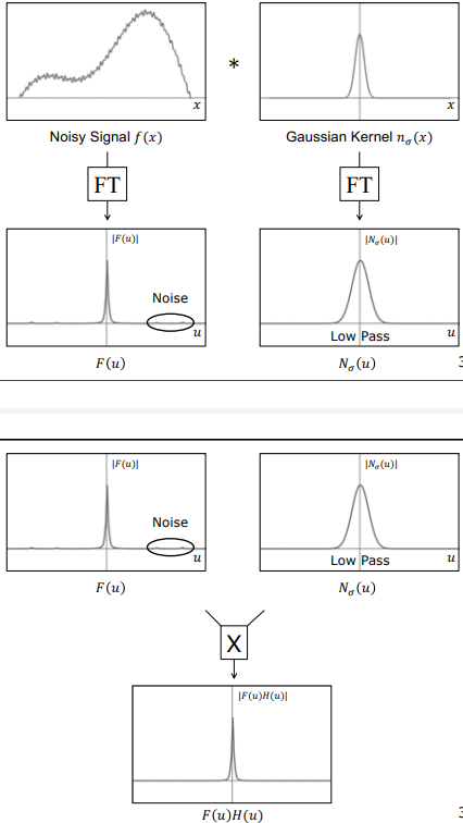
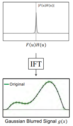
- Compute $F(u) = \mathcal{F}{f(x)}$ and $H(u) = \mathcal{F}{h(x)}$ using FFT ($O(N \log N)$).
- Perform element-wise multiplication $G(u) = F(u) \cdot H(u)$ ($O(N)$).
- Compute the Inverse FFT $g(x) = \mathcal{F}^{-1}{G(u)}$ ($O(N \log N)$).
This reduces computational complexity from $O(N^2)$ to $O(N \log N)$, providing enormous acceleration for large filter kernels and offering clear visual insight into which spatial frequencies a filter attenuates or passes.