Camera Response, HDR Imaging, and Nature’s Sensors
- 1. Camera Response Function and Radiometric Calibration
- 2. High Dynamic Range (HDR) Imaging
- 3. Nature’s Image Sensors and Biological Vision
1. Camera Response Function and Radiometric Calibration
While the relationship between the physical photon flux and the generated sensor charge is highly linear, consumer cameras output non-linear pixel intensities.
1.1 The Camera Response Function ($f$)
When light strikes a sensor pixel, the relationship between scene brightness and measured image intensity is guaranteed to be monotonic, but is rarely linear.
flowchart LR
    FLUX["Incoming Photon Flux (I)"] --> EXP["Pixel Linear Charge (B)<br/>B = I · e = I · (A · T)"]
    EXP --> ISP["Electronics & Image Signal Processor (ISP)<br/>(ADC, Demosaicing, Sharpening)"]
    ISP --> OUT["Non-Linear Output Intensity (M)<br/>M = f(B)"]

    style FLUX fill:#1a1a2e,stroke:#fff,color:#fff
    style EXP fill:#16213e,stroke:#4cc9f0,color:#fff
    style ISP fill:#0f3460,stroke:#f72585,color:#fff
    style OUT fill:#e94560,stroke:#06d6a0,color:#fff
Linear Exposure ($B$)
The raw intensity $B$ inside the pixel is strictly linear with respect to the incoming photon flux $I$ and the total exposure $e$. Exposure is the product of the aperture area $A$ (related to diameter $D$) and the integration time $T$:
$$B = I \times e = I \times (A \times T)$$
Electronic Modulation
Before being outputted as a digital measurement $M$, this linear charge $B$ undergoes electron-to-voltage conversion, Analog-to-Digital conversion (ADC), and several digital image signal processing (ISP) operations (such as demosaicing, sharpening, and contrast enhancement).
Non-Linear Squeezing (Gamma Curve)
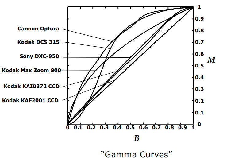
Camera manufacturers intentionally introduce a non-linear mapping function $f$ (known as the Gamma Curve or Gamma Function):
$$M = f(B)$$
The Squeezing Principle: Because digital image formats have a finite dynamic range (typically 8 bits per channel, 0 to 255), mapping linear intensities directly would waste precious numerical bits on bright highlights that the human eye cannot easily distinguish. Instead, $f$ compresses the bright, high-intensity regions (like clouds in the sky) while dedicating much higher numerical resolution to darker values, preserving critical shadow details.
1.2 Radiometric Calibration
For many quantitative computer vision applications (such as photometric stereo or shape from shading), the true linear scene irradiance must be recovered from the non-linear pixel values $M$. The process of finding and inverting this non-linear function $f$ is called radiometric calibration.
flowchart TD
    MAB["Standard Macbeth Color Chart<br/>(Neutral Gray Patches: 3.1% to 90.0% Reflectance)"] --> ILL["Uniform Distant Illumination<br/>(Linear Brightness B ∝ Reflectance)"]
    ILL --> CAP["Capture Single Test Frame<br/>(Normalize Peak Patch to 1.0)"]
    CAP --> CURVE["Plot Reflectance (B) vs Digital Intensity (M)<br/>(Reconstruct Response Function f)"]
    CURVE --> INV["Apply Inverse Response Function f⁻¹(M)<br/>(Recover True Linear Scene Irradiance B)"]

    style MAB fill:#1a1a2e,stroke:#4cc9f0,color:#fff
    style ILL fill:#16213e,stroke:#e94560,color:#fff
    style CAP fill:#0f3460,stroke:#f72585,color:#fff
    style CURVE fill:#e94560,stroke:#fff,color:#fff
    style INV fill:#06d6a0,stroke:#111,color:#000
Calibration Steps Using a Macbeth Chart
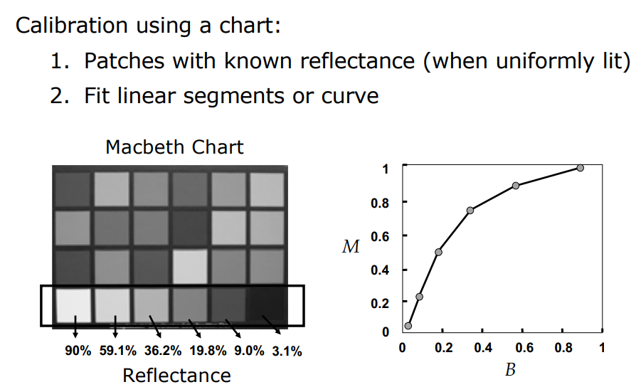
- Chart Selection: A standard Macbeth Chart contains a bottom row of neutral gray patches with precisely known physical reflectance values, spanning from 3.1% (dark patch) to 90.0% (bright patch).
- Uniform Illumination: The chart is illuminated using distant light sources, ensuring a perfectly uniform illumination over the entire surface.
- Reflectance Proportionality: Because illumination is constant, the true linear image brightness $B$ of each gray patch is directly proportional to its known physical reflectance, scaled by an unknown constant factor $k$ (which depends on light source intensity, camera gain, etc.): $$B \propto \text{Reflectance}$$
- Plotting and Inversion: A single image of the chart is captured. The brightest patch’s linear intensity is normalized to 1.0 to eliminate the unknown scale factor $k$.
- Curve Reconstruction: By plotting the known linear reflectances on the x-axis ($B$) and the measured digital pixel values on the y-axis ($M$), we reconstruct the camera’s response curve $f$.
Once $f$ is calibrated, we can linearize any subsequent image captured by the camera by passing the pixels through the inverse function $f^{-1}$, recovering true scene brightness up to a single scale factor:
$$B = f^{-1}(M)$$
2. High Dynamic Range (HDR) Imaging
Real-world environments exhibit an enormous range of light intensities that far exceed the 72 dB dynamic range of consumer sensors.
2.1 Exposure Bracketing
Exposure bracketing combines multiple frames of a static scene captured at different integration times to synthesize an image with a wider dynamic range.
flowchart TD
    subgraph Bracket ["Multi-Exposure Sequence"]
        E0["Frame M0 (Short Exposure e0)<br/>Captures Highlights (Window / Sky)"]
        E1["Frame M1 (Medium Exposure e1)<br/>Captures Mid-Tones"]
        E2["Frame M2 (Long Exposure e2)<br/>Captures Shadows"]
        E3["Frame M3 (Ultra Exposure e3)<br/>Captures Darkest Indoor Details"]
    end

    Bracket --> SUM["Linear Addition (Linearized Images)<br/>M_HDR = M0 + M1 + M2 + M3"]
    SUM --> TONE["Tone Mapping Algorithm<br/>(Compresses 10-bit / 1020 Range to 8-bit)"]
    TONE --> OUT["Final HDR Image<br/>(Full Detail in Highlights & Shadows)"]

    style Bracket fill:#1a1a2e,stroke:#4cc9f0,color:#fff
    style SUM fill:#16213e,stroke:#e94560,color:#fff
    style TONE fill:#0f3460,stroke:#f72585,color:#fff
    style OUT fill:#06d6a0,stroke:#111,color:#000
Multi-Exposure Sequence
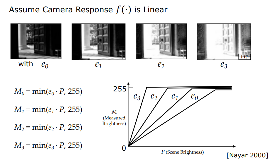
The camera captures a sequence of pictures with varying exposure times $e_0 < e_1 < e_2 < e_3$.
Mathematical Slices
For a scene point with true brightness $P$, the measured value in frame $i$ is capped at the sensor’s maximum saturation limit of 255:
$$M_i = \min(e_i \cdot P,\ 255)$$
- Short Exposure ($e_0$): Prevents highlights (such as a bright sky or window) from saturating, but leaves shadows completely black and noisy.
- Long Exposure ($e_3$): Floods the sensor with photons, capturing details in dark indoor shadows, but completely washes out and saturates outdoor regions.
Linear Addition
Assuming the camera response has been linearized ($f^{-1}$ applied), we sum these four exposures to generate an aggregate image:
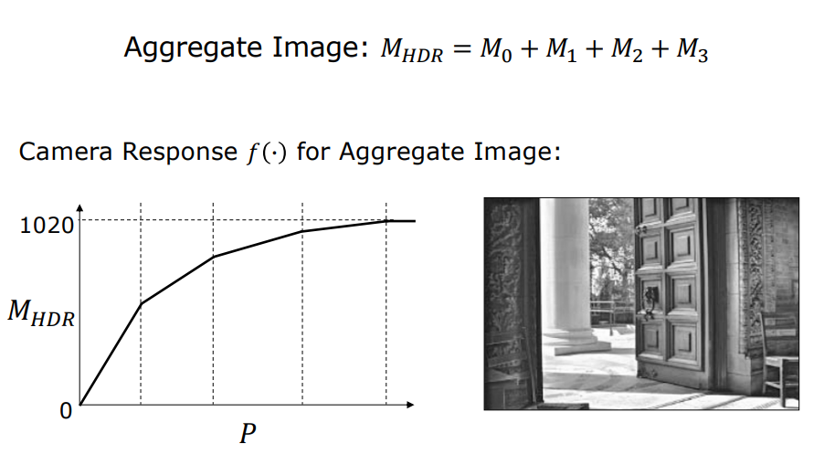
$$M_{\text{HDR}} = M_0 + M_1 + M_2 + M_3$$
The combined response function of this aggregate virtual camera compresses high scene intensities while maintaining high sensitivity in dark regions, yielding a maximum numerical value of 1020 ($4 \times 255$).
Tone Mapping
A tone mapping algorithm compresses this high-fidelity 10-bit output back down to standard 8-bit display formats, rendering both indoor shadows and outdoor skies with rich detail.
The Ghosting Artifact: Exposure bracketing works exceptionally well for static scenes but fails in dynamic environments. If an object (such as a bicyclist or pedestrian) moves during the multi-exposure capture sequence, it is recorded at different spatial coordinates in each frame. Adding these frames results in semi-transparent, duplicated overlapping copies in the final image, known as ghosting.
2.2 Single-Shot HDR via Assorted Pixels
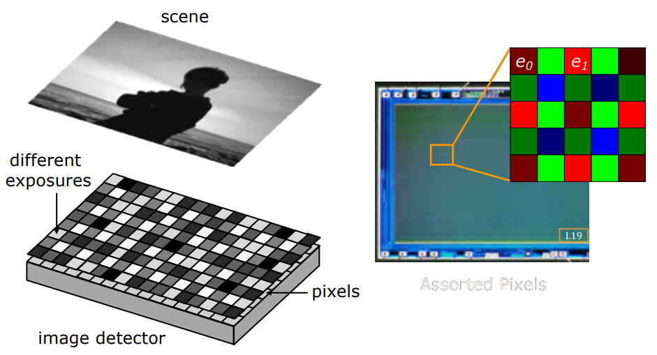
To capture HDR images of moving objects without ghosting, the entire dynamic range must be recorded in a single exposure. This is achieved using spatially varying pixel exposures (SVE), commonly referred to as Assorted Pixels.
- Pixel-Level Sensitivity Modulation: Instead of a uniform sensor where all pixels have identical sensitivity, an assorted pixel sensor features adjacent photodiodes with unequal light sensitivities.
- Optomechanical Implementation: This spatial variation is implemented by depositing micro-shades of varying optical transparencies directly over adjacent pixels or driving neighboring pixels with different integration times.
- Spatial Interpolation Pipeline:
- If a highly sensitive pixel saturates (clips to 255) under bright light, its less-sensitive (shaded) neighbor will not saturate and will successfully record the highlight detail.
- If a shaded pixel is too dark, its unshaded neighbor will capture clean, high-SNR details in the shadows.
- An interpolation algorithm then processes this patterned checkerboard image, predicting missing high-exposure and low-exposure values from neighboring pixels.
- Result: This single-shot HDR architecture produces full-color, high-contrast images with no motion artifacts and is widely used in modern smartphone camera modules.
3. Nature’s Image Sensors and Biological Vision
Over millions of years of evolution, nature has engineered visual systems that solve complex sensing challenges with elegant, non-traditional configurations.
3.1 Copilia’s Mechanical Scanning Eye
The marine crustacean Copilia (a microscopic plankton-like creature) possesses an eye that operates as an optomechanical scanner.
flowchart TD
    L1["Anterior Lens (Large Outer Lens)<br/>Fixed Focus to Internal Image Plane"] --> PLANE["Internal Image Plane<br/>(2D Optical Projection)"]
    PLANE --> L2["Mobile Posterior Lens + Single Biological Photoreceptor<br/>(Mechanically Scanned Back and Forth)"]
    L2 --> BRAIN["Copilia Brain<br/>(Reconstructs 2D Visual Field Over Time)"]

    style L1 fill:#1a1a2e,stroke:#4cc9f0,color:#fff
    style PLANE fill:#16213e,stroke:#e94560,color:#fff
    style L2 fill:#0f3460,stroke:#f72585,color:#fff
    style BRAIN fill:#06d6a0,stroke:#111,color:#000
- Optics: Each eye contains two lenses. A large, static outer anterior lens focuses light to form a two-dimensional image inside the head.
- Mechanical Scanning: Positioned behind this image plane is a mobile posterior lens paired with a single biological photoreceptor (a single-pixel sensor).
- Operation: Instead of utilizing a dense grid of millions of receptors, Copilia mechanically scans this posterior lens-receptor assembly back and forth across the anterior lens’s focal plane. By scanning the single pixel spatially over time, Copilia’s brain reconstructs a complete two-dimensional image of its environment.
3.2 Brittle Star (Ophiocoma wendtii): The Lens-Covered Body
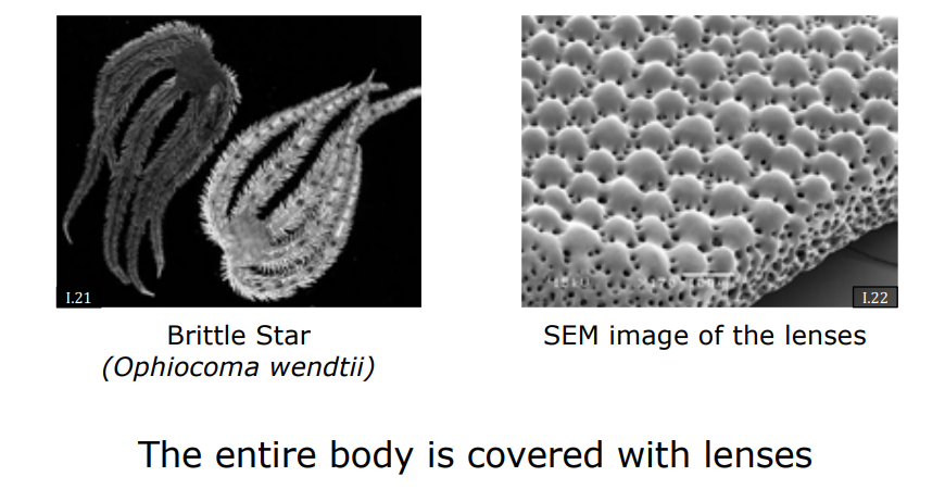
The Brittle Star (yılan yıldızı) is a marine creature with no brain and no traditional focal eyes. For decades, biologists were puzzled by its ability to navigate complex crevices and evade predators.
- The Discovery: Around 2001, scanning electron microscopy revealed that the entire calcitic skeletal body of the brittle star is covered with millions of tiny, highly transparent calcite crystal bumps.
- Optical Precision: Each crystal bump is an optically perfect microlens, measuring approximately 1/20 of a millimeter in diameter.
- The Flexible Camera: These calcitic microlenses focus light onto a bundle of nerve fibers running directly underneath them. The brittle star’s entire skeletal body effectively functions as a massive, flexible, curved image sensor, allowing it to perceive spatial distributions of light and shadow across its entire body.
3.3 Octopus Camouflage and Chromatophores
The skin of the octopus is a dynamic biological display and sensor array.
- Chromatophores: The skin contains millions of microscopic pigment-filled sacs called chromatophores.
- Neural Control: These sacs are directly controlled by surrounding muscle fibers. When the brain sends a neural impulse, the muscles contract or expand, changing the physical shape and surface area of the pigment sacs.
- Camouflage: By precisely modulating which colors are exposed, the octopus can match the texture, color, and reflectance of surrounding coral reefs or plants. This real-time camouflage is so perfect that the octopus remains completely invisible to predators even at close distances.
3.4 The Human Eye Blind Spot
In the human eye, the biological wiring of the retina creates a unique optical defect.
- The Optic Disk: All nerve impulses generated by the rods and cones travel along axons that gather at a single point on the retina: the optic disk.
- Zero Receptor Density: At this exit point, the optic nerve passes through the retinal layer to travel to the visual cortex of the brain. Because the nerve occupies this space, there is a physical patch on the retina that is completely devoid of rods and cones. This is the blind spot.
Neural Inpainting: We do not notice a physical hole in our daily field of view because our brain performs real-time spatial “inpainting” (interpolation), filling in missing visual information based on surrounding texture, color, and context.