Modern CNN Architectures: ResNet, Inception, MobileNet, EfficientNet

• ResNet: Deep Residual Networks
  • Residual Learning: Core Idea
  • Why ResNets Work?
  • Forward and Backward Propagation
  • Real-World Analogy
    • Variants of ResNet
• Inception and 1x1 Convolutions
  • Networks in Networks and 1x1 Convolutions
    • What is a 1x1 Convolution?
    • Why is it useful?
  • Inception Network
  • GoogLeNet and Inception Blocks
    • Structure of an Inception Block:
  • Improvements Over Time
• MobileNet and EfficientNet
  • MobileNet
    • Standard Convolution vs. Depthwise Separable Convolution
    • MobileNet Architecture (V1 Highlights)
  • EfficientNet
    • The Problem: How to Scale a CNN?
    • Compound Scaling: Efficient Strategy
    • Performance

ResNet: Deep Residual Networks

As neural networks became deeper, researchers observed a counterintuitive phenomenon: deeper networks often performed worse during training and testing compared to shallower ones. This degradation was not due to overfitting but rather an optimization issue.

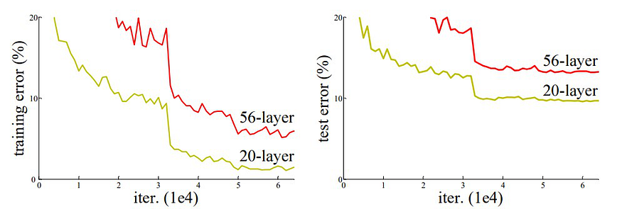
This problem is called the degradation problem. It shows that simply stacking more layers doesn't guarantee better accuracy — instead, it often leads to higher training error. This contradicts our expectations, since deeper models should be able to represent more complex functions.

To address this, ResNet introduced the concept of residual learning.

Residual Learning: Core Idea

Instead of learning a direct mapping $H(x)$, ResNet proposes to learn the residual function:

$$F(x)=H(x)-x\Rightarrow H(x)=F(x)+x$$

This reformulation allows the network to focus on learning the difference between the input and output, which is often easier to optimize.

The output of a residual block is:

$$\text{Output}=F(x,\{W_i\})+x$$

where $F(x,\{W_i\})$ is the output from a few stacked layers (e.g., 2 Conv-BN-ReLU layers) and $x$ is the original input. This addition is known as a skip connection or shortcut connection.

Here's the basic structure of a Residual Block:

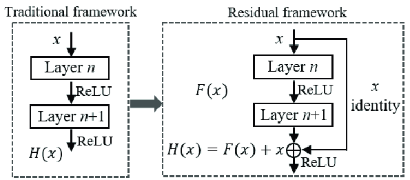
• If the input and output dimensions differ, a 1x1 convolution is used to match dimensions before addition.
• This structure allows gradients to flow more easily during backpropagation, mitigating the vanishing gradient problem.

Identity Shortcut Connection

This is the key innovation. By allowing the input to bypass intermediate layers, the model can preserve useful features, learn identity mappings when needed, and avoid overfitting.

Shortcut types:

• Identity shortcut: When input and output dimensions match
• Projection shortcut: 1x1 convolution used to match shapes

Why ResNets Work?

1. Improved Gradient Flow: Easier to train deep networks due to unblocked gradient paths
2. Easier Optimization: Residual mapping simplifies the learning process
3. Deeper Networks: Can train very deep networks (e.g., ResNet-152) without degradation
4. Better Generalization: Performs well across image classification, detection, segmentation

Forward and Backward Propagation

In a residual block, during forward propagation, the shortcut allows direct data flow from earlier layers. In backward propagation, the gradient can pass through both the residual path and shortcut connection, reducing gradient vanishing.

Let’s say the loss gradient is $\partial L/\partial y$. Then:

$$\frac{\partial L}{\partial x}=\frac{\partial L}{\partial y}\cdot (\frac{\partial F}{\partial x}+I)$$

Here, $I$ is the identity matrix, ensuring that gradient doesn’t vanish even if $\partial F/\partial x$ becomes small.

Real-World Analogy

Imagine you’re assembling a piece of furniture using instructions. Instead of reading and understanding every step from scratch (direct mapping), you compare each step with what you’ve already done (residual comparison). It’s easier to notice what's missing and fix it.

Variants of ResNet

• ResNet-18, 34, 50, 101, 152: Increasing depth
• ResNeXt: Groups of convolutions
• Pre-activation ResNet: Moves BN and ReLU before convolutions

Inception and 1x1 Convolutions

Networks in Networks and 1x1 Convolutions

In 2014, the "Network in Network" architecture introduced the idea of using 1x1 convolutions — a surprisingly powerful and efficient technique in modern CNNs.

What is a 1x1 Convolution?

• A 1x1 convolution applies a filter of size $1\times 1$ across all input channels.
• Though the spatial dimension ($1x1$) seems trivial, it processes channel-wise information and mixes features across depth.

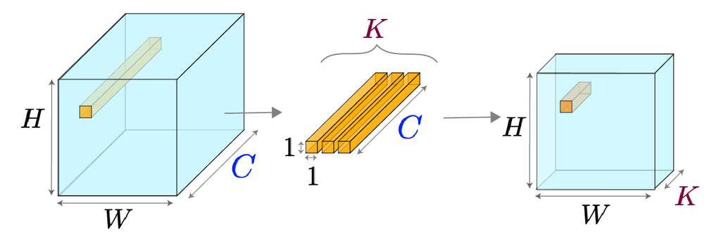
Let’s assume an input of shape $H\times W\times C\_in$. Applying $N$ 1x1 filters produces an output of shape $H\times W\times N$.

Why is it useful?

• Dimensionality Reduction: You can reduce the number of channels before applying computationally expensive filters (e.g., 3x3, 5x5), reducing the model size and speed requirements.
• Increase Non-Linearity: When combined with non-linear activations (like ReLU), it increases the representational power of the network.
• Lightweight Computation: Compared to a standard 3x3 convolution with the same input/output dimensions, the FLOPs (floating point operations) required are significantly lower.

Intuition:

Think of 1x1 convolution as a way to relearn combinations of channels at each spatial location. It’s like assigning weights to each feature and mixing them in a smart way — like forming new meanings from known "ingredients."

Inception Network

CNNs originally used sequential layers — stacking 3x3 or 5x5 filters one after another. But why settle for a single filter size?

Some patterns might be better captured with:

• 1x1 (fine details)
• 3x3 (mid-level features)
• 5x5 (larger context)

Key Insight:

Why not apply all of them in parallel, and let the network decide which one is best?

That’s the core idea behind the Inception Module.

Problem:

Applying multiple large filters in parallel increases computation exponentially.

GoogLeNet and Inception Blocks

The GoogLeNet (Inception-v1) architecture introduced the Inception module to allow multi-scale feature extraction while keeping the computation affordable.

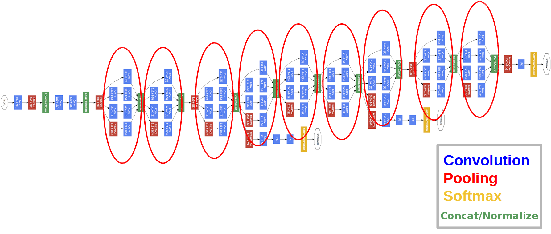
Structure of an Inception Block:

Each Inception block has multiple branches:

• 1x1 convolution
• 1x1 → 3x3 convolution
• 1x1 → 5x5 convolution
• 3x3 max pooling → 1x1 convolution

Notice how each expensive convolution is preceded by a 1x1 convolution for dimensionality reduction.

Advantages:

• Parameter Efficiency: Fewer parameters than naïvely stacking all filters.
• Rich Feature Learning: Learns features at multiple receptive fields simultaneously.
• Parallelism: More effective than deeper or wider models with uniform layers.

Example:

Assume an input of size $28\times 28\times 192$. After passing through an Inception module, we may get something like:

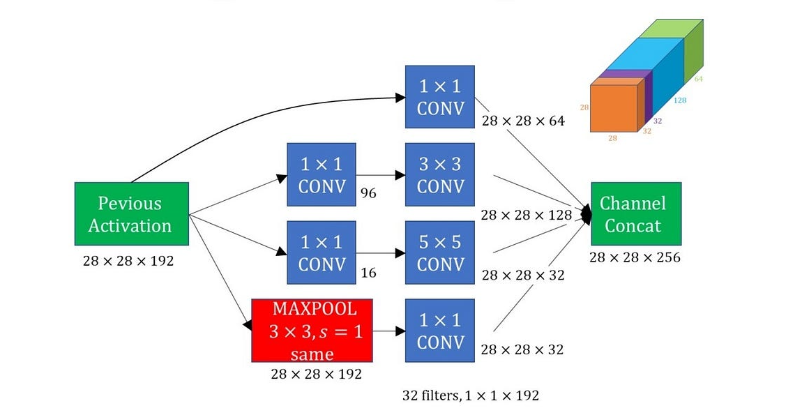
• 1x1 branch → 64 channels
• 3x3 branch → 128 channels
• 5x5 branch → 32 channels
• Pooling branch → 32 channels
• Total output depth: 256

Improvements Over Time

GoogLeNet inspired many improved versions:

• Inception v2/v3: Factorization of convolutions (e.g., 5x5 → two 3x3 layers)
• Inception v4: Combined ideas from ResNet and Inception (e.g., Inception-ResNet)
• Use of BatchNorm and Auxiliary Classifiers

These tricks improved accuracy without dramatically increasing parameters.

The Inception architecture was a major leap forward in CNN design:

• It introduced the concept of multi-path architectures
• Emphasized computational efficiency
• Leveraged 1x1 convolutions to control model complexity

This paved the way for even more efficient models like MobileNet and EfficientNet.

MobileNet and EfficientNet

MobileNet

As deep learning models became larger and deeper, they demanded more memory and computation — not ideal for mobile or embedded devices. MobileNet, introduced by Google in 2017, addressed this challenge by proposing a highly efficient architecture using depthwise separable convolutions.

Standard Convolution vs. Depthwise Separable Convolution

Let’s recall the standard convolution:

Given an input of size $H\times W\times Din$, applying $N$ filters of size $K\times K\times D$in produces an output of size $H^{\prime }\times W^{\prime }\times N$.

• Computation Cost: $$K\cdot K\cdot D_{in}\cdot N\cdot H^{\prime }\cdot W^{\prime }$$

MobileNet factorizes this into two steps:

1. Depthwise Convolution:
   Apply one filter per input channel — no cross-channel combination.
   Cost:

   $$K\cdot K\cdot D_{in}\cdot H^{\prime }\cdot W^{\prime }$$

2. Pointwise Convolution (1x1):
   Mix the depthwise output with $N$ 1x1 filters.
   Cost: $$D_{in}\cdot N\cdot H^{\prime }\cdot W^{\prime }$$

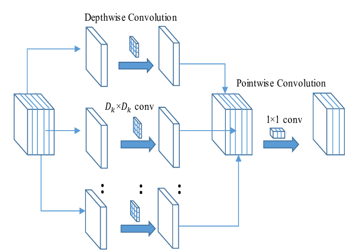
✅ Total Cost:

$$K^2\cdot D_{in}\cdot H^{\prime }\cdot W^{\prime }+D_{in}\cdot N\cdot H^{\prime }\cdot W^{\prime }$$

which is ~9x less than standard convolution when $K=3$.

MobileNet Architecture (V1 Highlights)

MobileNetV1 is built by stacking depthwise separable convolutions instead of regular ones. It also introduces:

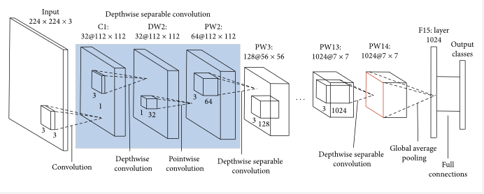
• Width Multiplier (α): Shrinks the number of channels (e.g., α=0.75 reduces model size).
• Resolution Multiplier (ρ): Reduces input image size to further save computation.

Together, these enable a trade-off between accuracy and resource usage.

MobileNet is often used as a backbone in real-time applications (e.g., object detection on smartphones, AR apps).

EfficientNet

Introduced in 2019 by Google AI, EfficientNet pushes the boundary of model performance by scaling neural networks systematically.

The Problem: How to Scale a CNN?

You can make a CNN more powerful by:

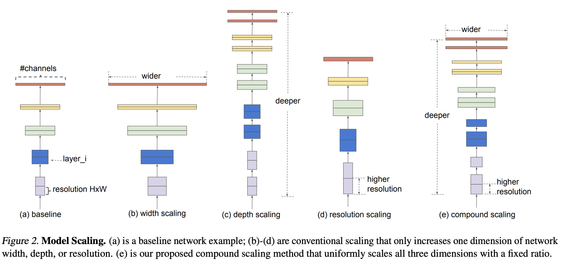
• Increasing depth (more layers)
• Increasing width (more channels)
• Increasing resolution (larger input images)

But how much of each?

Compound Scaling: Efficient Strategy

Instead of arbitrarily scaling one dimension, EfficientNet introduces a compound coefficient (ϕ) that balances all three:

$$\begin{array}{rl}\text{depth:}& d={\alpha }^{\varphi }\\ \text{width:}& w={\beta }^{\varphi }\\ \text{resolution:}& r={\gamma }^{\varphi }\\ \text{subject to:}& \alpha \cdot {\beta }^2\cdot {\gamma }^2\approx 2\end{array}$$

• ϕ controls the available resources (e.g., more computation).
• α, β, γ are constants determined via grid search.

Performance

EfficientNet models (B0 to B7) are built on the same base architecture (EfficientNet-B0), with progressively larger values of ϕ.

• EfficientNet-B0: baseline
• EfficientNet-B1 to B7: scaled versions with increasing capacity

✅ Result:
EfficientNet achieves better accuracy with fewer parameters compared to deeper networks like ResNet-152 or Inception-v4.

Both architectures represent the evolution of CNN design towards compact, fast, and powerful models — a necessary shift for real-world AI deployment.