Object Localization and Detection

• Object Localization
  • Output Vector
  • Loss Function
• Landmark Detection
  • Output Representation
  • Loss Function
• Object Detection
  • Example
  • Compared to Localization
  • Model Output Structure
• Sliding Window Approach and Its Convolutional Implementation
  • Limitations of Naive Sliding Windows
  • Convolutional Implementation of Sliding Windows
  • Use in Modern Architectures
    • Understanding the YOLO (You Only Look Once) Architecture
      • How Does YOLO Work?
    • SSD (Single Shot MultiBox Detector)
  • Summary

Object Localization

Object localization is the task of identifying the presence of an object in an image and determining its position using a bounding box.

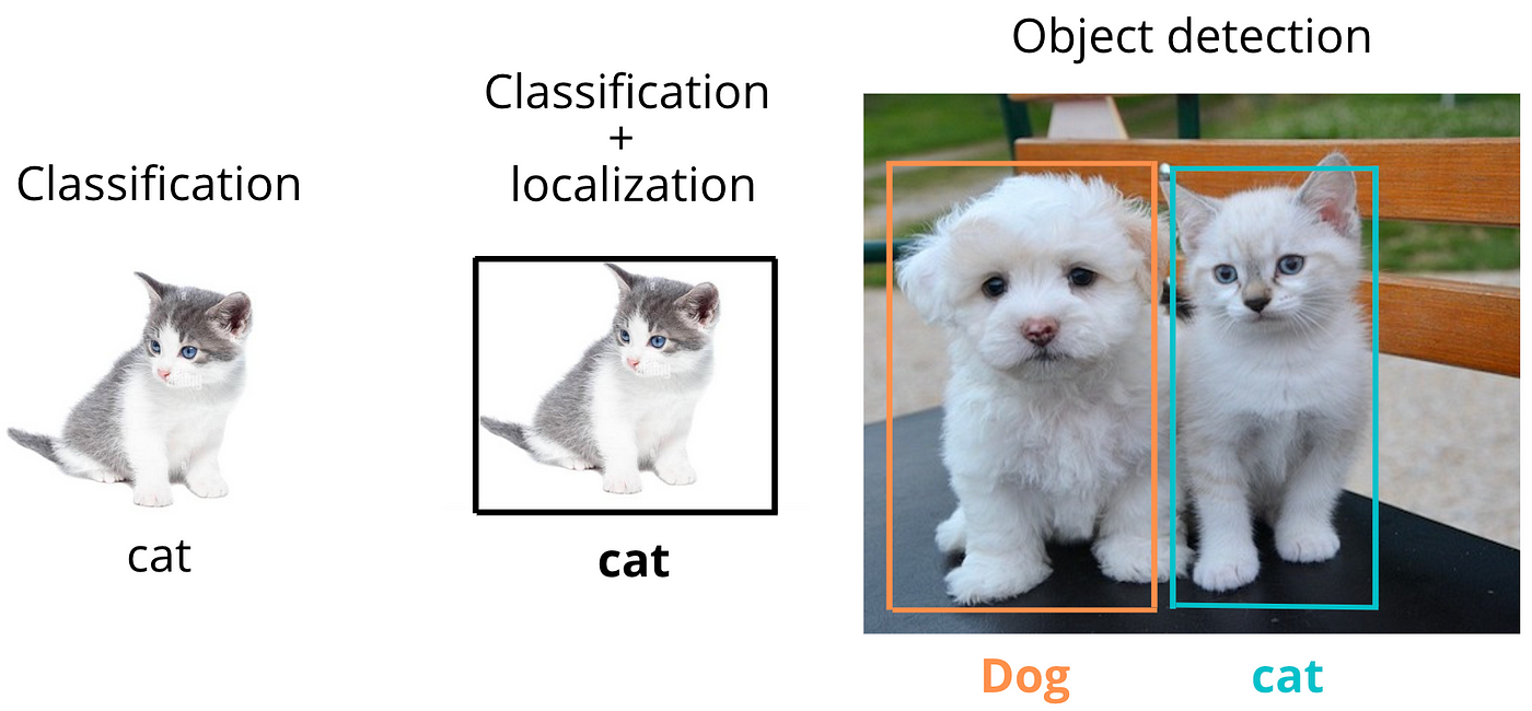
It’s one step more complex than image classification, which only tells what is in the image, not where it is.

Given an image, object localization aims to:

• Classify the object (e.g., cat, dog, car).
• Return the bounding box coordinates around the object: $$(x_{\text{min}},y_{\text{min}},x_{\text{max}},y_{\text{max}})\text{or}(x,y,w,h)$$

Where:

• $(x,y)$: center of the bounding box
• $w,h$: width and height of the box

Output Vector

If you're using a neural network for localization, the output vector might be:

$$\text{Output}=[p_c,x,y,w,h,c_1,c_2,...,c_n]$$

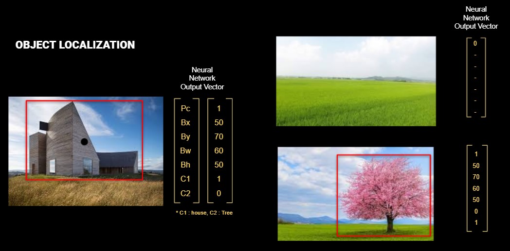
Where:

• $p_c$: Probability that an object exists in the image
• $x,y,w,h$: Bounding box
• $c_i$: Class probabilities (e.g., cat = 0.8, dog = 0.2)

If the object whose class is defined cannot be detected on the image, $p_c$ will be $0$. In the case where $p_c$ is $0$, the bounding box values ​​($x,y,w,h$) and class values ​​are insignificant in the vector. This means that they are not included when calculating the Loss function.

Loss Function

A multi-part loss is generally used for localization:

• Localization loss (coordinate regression): Measures error in predicted box location
• Confidence loss (objectness): Measures error in object existence
• Classification loss: Measures class prediction error

Example (simplified version as in YOLO):

$$\mathcal{L}={\lambda }_{\text{coord}}\cdot \sum _i{1}_i^{\text{obj}}\left[(x_i-{\hat{x}}_i{)}^2+(y_i-{\hat{y}}_i{)}^2+(w_i-{\hat{w}}_i{)}^2+(h_i-{\hat{h}}_i{)}^2\right]+\text{classification loss}$$

Landmark Detection

Landmark detection (also called keypoint detection) involves detecting specific key locations on an object. Unlike bounding boxes, keypoints give finer-grained localization.

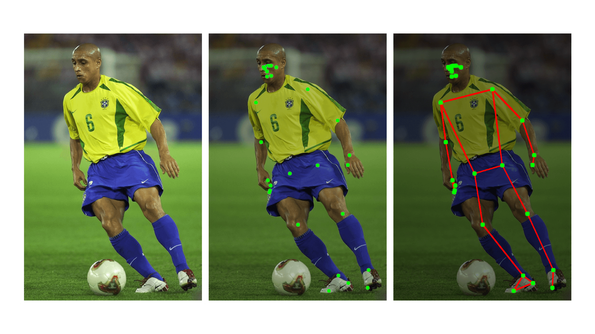
Example

• Face recognition: Eyes, nose tip, mouth corners
• Hand detection: Fingertips and joints
• Medical imaging: Identifying organ boundaries

Output Representation

If we detect $K$ landmarks:

$$\text{Output}=[x_1,y_1,x_2,y_2,...,x_K,y_K]$$

Each pair represents the $(x,y)$ coordinate of a keypoint like knee point or ear point.

Loss Function

The typical loss for landmark detection:

$${\mathcal{L}}_{\text{keypoints}}=\sum _{k=1}^K\left[(x_k-{\hat{x}}_k{)}^2+(y_k-{\hat{y}}_k{)}^2\right]$$

Object Detection

Object detection combines classification and localization — but now for multiple objects in the same image.

Example

In a single street photo:

• Detect a car (class = car, bounding box)
• Detect a pedestrian (class = human, bounding box)
• Detect a stop sign (class = sign, bounding box)

Compared to Localization

Model Output Structure

We divide the image into an $S\times S$ grid. For each grid cell, predict:

• $B$ bounding boxes
• Confidence score
• Class probabilities

$$\text{Output Tensor}=S\times S\times (B\cdot 5+C)$$

Where:

• Each box includes $[p_c,x,y,w,h]$. $5$ means this vector.
• $C$: number of classes

Sliding Window Approach and Its Convolutional Implementation

The sliding window technique is a classic method in computer vision used for object detection. The core idea is to take a fixed-size rectangular window and slide it across the input image, systematically checking each region to see whether it contains the object of interest.

At each window position, the cropped image region is passed to a classifier (e.g., SVM, logistic regression, or a small CNN) to determine whether it contains an object. This window "slides" over the image both horizontally and vertically, often with some stride value, producing many cropped regions.

It converts a classification model into a localization tool by brute-force scanning over all possible positions.

Limitations of Naive Sliding Windows

Although conceptually simple, the naive sliding window method has serious drawbacks:

1. High Computational Cost

• For an image of size $W\times H$, using a window of size $w\times h$ with stride $s$, the number of windows is: $$\left(\frac{W-w}{s}+1\right)\cdot \left(\frac{H-h}{s}+1\right)$$ This can result in thousands of regions even for medium-sized images.
• Each window requires a separate forward pass through the classifier network, resulting in massive redundancy since overlapping windows share most of their pixels.

2. Difficulty in Handling Multiple Scales

• Objects in an image can appear at different scales and aspect ratios.
• To address this, either the image must be resized many times or the window size must vary — both of which further increase computation.

3. Fixed Window Shape

• Sliding windows generally use a fixed aspect ratio and size, which makes them less effective for detecting objects with irregular shapes.

Convolutional Implementation of Sliding Windows

To overcome these inefficiencies, modern approaches use the convolutional structure of neural networks to implement the sliding window more efficiently.

Key Insight: Convolutions as Shared Computation

Instead of running the classifier separately on each window, we can:

• Pass the entire image through the convolutional layers of a CNN once
• These layers produce a feature map where each spatial position encodes information about a local receptive field (i.e., a subregion of the image)
• This naturally simulates a sliding window operation

Then, we apply 1x1 convolutions or fully connected layers converted into convolutions over the feature map to produce dense predictions for object presence.

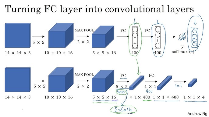
Fully Connected Layer to Convolution

A fully connected layer expecting a flattened $N\times N\times D$ input can be rewritten as a 1x1 convolution over a $N\times N\times D$ feature map:

• Each position in the resulting output map corresponds to a specific receptive field on the original image
• This effectively implements classification over many regions at once, reusing shared computation

Use in Modern Architectures

Understanding the YOLO (You Only Look Once) Architecture

YOLO (You Only Look Once) is a real-time object detection system that reframes object detection as a single regression problem, rather than a classification or region proposal problem. Instead of scanning the image multiple times or generating multiple proposals, YOLO sees the entire image only once and directly outputs bounding boxes and class probabilities in a single evaluation.

This end-to-end architecture enables extremely fast inference and is designed for real-time applications such as self-driving cars, robotics, surveillance, and augmented reality.

How Does YOLO Work?

At a high level, YOLO divides the input image into a fixed-size grid and makes predictions for each grid cell. Let’s go through each part of the architecture:

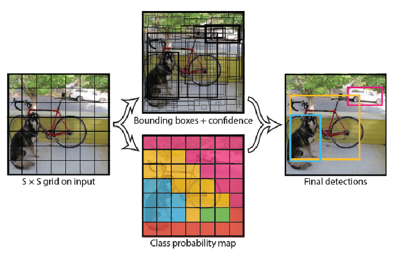
1. Image Grid Division

• The input image is divided into an $S\times S$ grid (e.g., $7\times 7$).
• Each grid cell is responsible for detecting objects whose center falls inside the cell.

2. Bounding Box Predictions

Each grid cell predicts:

• $B$ bounding boxes (typically $B=2$)
• For each box:
  • $x,y$: coordinates of the box center (relative to the grid cell)
  • $w,h$: width and height of the box (relative to the whole image)
  • $p_c$: confidence score = $P(\text{object})\times \text{IoU}\text{pred,truth}$

3. Class Probabilities

• Each grid cell also predicts $C$ conditional class probabilities:

  $$P(\text{class}\_i\mid \text{object})\text{for }i=1,\dots ,C$$

• These probabilities are class probabilities conditioned on the presence of an object in the cell.

4. Final Predictions

• The total output per grid cell is: $$B\times [p_c,x,y,w,h]+C$$ For example, with $S=7$, $B=2$, $C=20$, the total prediction tensor size is: $$7\times 7\times (2\times 5+20)=7\times 7\times 30$$

Why Is It Called “You Only Look Once”?

Traditional detection pipelines involve:

• Generating region proposals (like in R-CNN)
• Running a CNN on each region
• Performing classification and box regression separately

YOLO unifies this pipeline into a single CNN pass, hence the name “You Only Look Once”. The model sees the full image context and outputs all bounding boxes and class scores in one go.

SSD (Single Shot MultiBox Detector)

• Detects objects at multiple scales using feature maps from different layers
• Uses convolutional layers to predict class and box offsets at every location in the feature map

Summary

By understanding this transition from brute-force scanning to convolutional prediction, we appreciate how convolutional networks not only recognize what is in an image but also where, enabling scalable object detection.